Entropy-Randomized Clustering

Abstract

This paper proposes a clustering method based on a randomized representation of an ensemble of possible clusters with a probability distribution. The concept of a cluster indicator is introduced as the average distance between the objects included in the cluster. The indicators averaged over the entire ensemble are considered the latter’s characteristics. The optimal distribution of clusters is determined using the randomized machine learning approach: an entropy functional is maximized with respect to the probability distribution subject to constraints imposed on the averaged indicator of the cluster ensemble. The resulting entropy-optimal cluster corresponds to the maximum of the optimal probability distribution. This method is developed for binary clustering as a basic procedure. Its extension to t-ary clustering is considered. Some illustrative examples of entropy-randomized clustering are given.

1. Introduction

Cluster analysis of different objects is a branch of machine learning where the teacher’s labels are replaced by some internal characteristics of objects or external characteristics of clusters. The internal ones include the distances between objects within the cluster [1,2] and the similarity of objects [3]. Among the external characteristics, we mention the distances between the clusters [4]. As a mathematical problem, clustering has no universal statement. Therefore, clustering algorithms are often heuristic [5,6].

A highly developed area of research is cluster analysis of large text arrays. As a rule, latent features are first detected based on latent semantic analysis [7]. Subsequently, they are used for clustering [8,9]. Recently, there have appeared works based on the concept of ensemble clustering [10,11].

Most clustering algorithms involve the distance between objects, measured in an accepted metric, and enumerative search algorithms with heuristic control [12]. Clustering results significantly depend on the metric. Therefore, it is very important to quantify the quality of clustering [13,14,15].

This paper proposes a clustering method based on a randomized representation of an ensemble of possible clusters with a probability distribution [16]. The concept of a cluster indicator is introduced as the average distance between the objects included in the cluster. Since clusters are treated as random objects, the indicators averaged over the entire ensemble are considered the latter’s characteristics. The optimal distribution of clusters is determined using the randomized machine learning approach: an entropy functional is maximized with respect to the probability distribution subject to constraints imposed on the averaged indicator of the cluster ensemble. The resulting entropy-optimal cluster corresponds in size and composition to the maximum of the optimal probability distribution.

The optimal distribution of clusters is based on the method of the randomized maximum entropy estimation (MEE method) described in [16]. The method turns out to be effective in many machine learning and data mining problems. Among other features, it introduces the problem of entropy-randomized clustering. This article is devoted to a more detailed presentation of this problem in terms of proving the convergence of the multiplicative algorithm and the logical scheme of the clustering procedures.

2. An Indicator of Data Matrices

Consider a set of n objects characterized by row vectors ${\mathbf{x}}^{\left(1\right)},\cdots ,{\mathbf{x}}^{\left(n\right)}$ from the feature space $R^m$. Using these vectors, we construct the following n-row matrix:

$$X^{(1,\cdots ,n)}=\left(\begin{array}{c}{\mathbf{x}}^{\left(1\right)}\\ \cdots \\ {\mathbf{x}}^{\left(n\right)}\end{array}\right).$$

(1)

Let the distance between the ith and jth rows be defined as

$$\varrho ({\mathbf{x}}^{\left(i\right)},{\mathbf{x}}^{\left(j\right)})={\parallel {\mathbf{x}}^{\left(i\right)}-{\mathbf{x}}^{\left(j\right)}\parallel }_{R^m},$$

(2)

where ${\parallel •\parallel }_{R^m}$ denotes an appropriate metric in the feature space $R^m$. Next, we construct the distance matrix

$$D_{(n\times n)}=\left(\begin{array}{cccc}0& \varrho ({\mathbf{x}}^{\left(1\right)},{\mathbf{x}}^{\left(2\right)})& \cdots & \varrho ({\mathbf{x}}^{\left(1\right)},{\mathbf{x}}^{\left(n\right)})\\ \varrho ({\mathbf{x}}^{\left(2\right)},{\mathbf{x}}^{\left(1\right)})& 0& \cdots & \varrho ({\mathbf{x}}^{\left(2\right)},{\mathbf{x}}^{\left(n\right)})\\ \cdots & \cdots & \cdots \\ \varrho ({\mathbf{x}}^{\left(n\right)},{\mathbf{x}}^{\left(1\right)})& \varrho ({\mathbf{x}}^{\left(n\right)},{\mathbf{x}}^{\left(2\right)})& \cdots & 0\end{array}\right).$$

(3)

We introduce an indicator of the matrix $X^{(1,\cdots ,n)}$ as the average value of the elements of the distance matrix $D$:

$$\mathrm{d}\mathrm{i}\mathrm{s}\left(X\right)=\frac{2}{n(n-1)}\sum _{(i,j)=1,j\ne i}^n\varrho ({\mathbf{x}}^{\left(i\right)},{\mathbf{x}}^{\left(j\right)}).$$

(4)

Below, the objects will be included in clusters depending on the distances in (2). Therefore, the important characteristics of the matrix $X^{(1,\cdots ,n)}$ are the minimum and maximum elements of the distance matrix $D$:

$$\mathrm{i}\mathrm{n}\mathrm{f}\left(D\right)=\underset{i,j}{min}\varrho ({\mathbf{x}}^{\left(i\right)},{\mathbf{x}}^{\left(j\right)}),\mathrm{s}\mathrm{u}\mathrm{p}\left(D\right)=\underset{i,j}{max}\varrho ({\mathbf{x}}^{\left(i\right)},{\mathbf{x}}^{\left(j\right)}).$$

(5)

Note that the elements of the distance matrices of the clusters belong to the interval $\mathcal{I}=\left[\mathrm{i}\mathrm{n}\mathrm{f}\right(D),\mathrm{s}\mathrm{u}\mathrm{p}(D\left)\right].$

3. Randomized Binary Clustering

The binary clustering problem is to arrange n objects between two clusters ${\mathcal{K}}_{\left(s^{*}\right)}$ and ${\mathcal{K}}_{(n-s^{*})}$ of sizes $s^{*}$ and $(n-s^{*}),$ respectively:

$$\begin{array}{ccc}\hfill & & {\mathcal{K}}_{\left(s^{*}\right)}=\{i_1,\cdots ,i_{s^{*}}\},{\mathcal{K}}_{(n-s^{*})}=\{j_1,\cdots ,j_{(n-s^{*})}\};\hfill \\ & & (i_1,\cdots ,i_s)\ne (j_1,\cdots ,j_{(n-s^{*})}),(i_{\alpha },j_{\beta })=\overline{1,n},\alpha =\overline{1,s^{*}},\beta =\overline{1,n-s^{*}}.\hfill \end{array}$$

(6)

It is required to find the size $s^{*}$ and composition $\{i_1,\cdots ,i_{s^{*}}\}$ of the cluster ${\mathcal{K}}_{\left(s^{*}\right)}.$

For each fixed cluster size $s,$ the clustering procedure consists of selecting a submatrix $X_{\left(s\right)}$ of some $s<n$ rows from the matrix $X^{(1,\cdots ,n)}.$ If the matrix $X_{\left(s\right)}$ is selected, then the remaining rows form the matrix $X_{(n-s)}$ and the set of their numbers form the cluster ${\mathcal{K}}_{(n-s)}.$

Clearly, the matrix $X_{\left(s\right)}$ can be formed from the rows of the original matrix $X^{(1,\cdots ,n)}$ in $C_s^n$ different ways (the number of s-combinations from the set of n elements). For each of them, the matrices $X_{(n-s)}$ can be formed in a corresponding number of ways.

According to the principle of randomized binary clustering, the matrix $X_{\left(s\right)}$ is a random object and its particular images are the realizations of this object. The sets of its elements and the number of rows s are therefore random.

A realization of the random object is a set of row vectors from the original matrix:

$$X_{\left(s\right)}=X_{\left(s\right)}^{(i_1,\cdots ,i_s)}=\left(\begin{array}{c}{\mathbf{x}}^{\left(i_1\right)}\\ \cdots \\ {\mathbf{x}}^{\left(i_s\right)}\end{array}\right).$$

(7)

We renumber this set as follows:

$$\{i_1,\cdots ,i_s\}\to k=\overline{1,K\left(s\right)};K\left(s\right)=C_s^n.$$

(8)

Thus, the randomization procedure yields a finite ensemble of the form

$${\mathcal{X}}_{\left(s\right)}=\left\{X_{\left(s\right)}^1,\cdots ,X_{\left(s\right)}^{K\left(s\right)}\right\}.$$

(9)

Recall that the matrices in this ensemble are random. Hence, we assume the existence of probabilities $p(s,k)$ for realizing the ensemble elements, where s and k denote the cluster size and cluster realization number, respectively:

$$X_{\left(s\right)}^{\left(k\right)}\mathrm{w}\mathrm{i}\mathrm{t}\mathrm{h}\mathrm{p}\mathrm{r}\mathrm{o}\mathrm{b}\mathrm{a}\mathrm{b}\mathrm{i}\mathrm{l}\mathrm{i}\mathrm{t}\mathrm{y}p(s,k),s=\overline{1,(n-1)},k=\overline{1,K}.$$

(10)

Then, the randomized binary clustering problem reduces to determining a discrete probability distribution $p(s,k),(s=\overline{1,(n-1)},k=\overline{1,K})$, which is appropriate in some sense.

Let such a function $p^{*}(s,k)$ be obtained; according to the general variational principle of statistical mechanics, the realized matrix will be

$$X_{\left(s^{*}\right)}^{\left(k^{*}\left(s^{*}\right)\right)},\mathrm{w}\mathrm{h}\mathrm{e}\mathrm{r}\mathrm{e}{k}^{*}\left(s^{*}\right)=\underset{s,k}{max}{p}^{*}(s,k).$$

(11)

This matrix corresponds to the most probable cluster of $s^{*}$ objects with the numbers

$${\mathcal{K}}_1^{*}=\{i_1^{*},\cdots ,i_{s^{*}}^{*}\}\to k^{*}\left(s^{*}\right).$$

(12)

The other cluster consists of the remaining $(n-s^{*})$ objects with the numbers

$${\mathcal{K}}_2^{*}=\{j_1^{*},\cdots ,j_{(n-s^{*})}^{*}\},(j_1^{*},\cdots ,j_{(n-s^{*})}^{*})\ne (i_1^{*},\cdots ,i_{s^{*}}^{*}).$$

(13)

Generally speaking, there are many such clusters but they all contain the same $(n-s^{*})$ objects.

4. Entropy-Optimal Distribution ${\mathit{p}}^{*}(\mathit{s},\mathit{k})$

Consider the cluster ${\mathcal{K}}_1$ of size $s,$ the associated matrix

$$X_{\left(s\right)}^{(i_1,\cdots ,i_s)}=\left(\begin{array}{c}{\mathbf{x}}^{\left(i_1\right)}\\ \cdots \\ {\mathbf{x}}^{\left(i_s\right)}\end{array}\right)=X_{\left(s\right)}^{\left(k\right)},\{i_1,\cdots ,i_s\}\to k,$$

(14)

and the distance matrix

$$D_{\left(s\right)}^{(i_1,\cdots ,i_s)}=\left(\begin{array}{cccc}0& {\varrho }^{\left(k\right)}({\mathbf{x}}^{i_1},{\mathbf{x}}^{i_2})& \cdots & {\varrho }^{\left(k\right)}({\mathbf{x}}^{i_1},{\mathbf{x}}^{i_s})\\ \cdots & \cdots & \cdots & \\ {\varrho }^{\left(k\right)}({\mathbf{x}}^{i_s},{\mathbf{x}}^{i_1})& {\varrho }^{\left(k\right)}({\mathbf{x}}^{i_s},{\mathbf{x}}^{i_2})& \cdots & 0\end{array}\right)=D_{\left(s\right)}^{\left(k\right)}.$$

(15)

We define the matrix indicator in (4) for the cluster ${\mathcal{K}}_s$ as

$$\mathrm{d}\mathrm{i}\mathrm{s}(X_{\left(s\right)}^{\left(k\right)})=\frac{2}{s(s-1)}\sum _{(t,h)=1,t\ne h}^s{\varrho }^{\left(k\right)}({\mathbf{x}}^{i_t},{\mathbf{x}}^{i_h}).$$

(16)

Since the matrices $X_{\left(s\right)}^{\left(k\right)}$ are supposed random objects, their ensemble has a probability distribution $p(s,k)$. We introduce the average indicator in the form

$$\mathcal{M}\{\mathrm{d}\mathrm{i}\mathrm{s}(X_{\left(s\right)}^{\left(k\right)})\}=\sum _{s=1}^{n-1}\sum _{k=1}^{K\left(s\right)}p(s,k)\mathrm{d}\mathrm{i}\mathrm{s}(X_{\left(s\right)}^{\left(k\right)}).$$

(17)

For determining the discrete probability distribution $p(s,k),$ we apply randomized machine learning with the Boltzmann–Shannon entropy functional [17]:

$${\mathcal{H}}_B\left[p(s,k)\right]=-\sum _{s=1}^{n-1}\sum _{k=1}^{K\left(s\right)}p(s,k)lnp(s,k)\Rightarrow max$$

(18)

subject to the constraints

$$0\le p(s,k)\le 1,s=\overline{1,(n-1)},k=\overline{1,K\left(s\right)},$$

(19)

$$\mathrm{i}\mathrm{n}\mathrm{f}\left(D\right)\le \sum _{s=1}^{n-1}\sum _{k=1}^{K\left(s\right)}p(s,k)\mathrm{d}\mathrm{i}\mathrm{s}(X_{\left(s\right)}^{\left(k\right)})\le \mathrm{s}\mathrm{u}\mathrm{p}\left(D\right).$$

(20)

Here, the lower $inf\left(D\right)$ and upper $sup\left(D\right)$ bounds for the elements of the distance matrix are given by (5); the indicator $\mathrm{d}\mathrm{i}\mathrm{s}(X_{\left(s\right)}^{\left(k\right)})$ is given by (16).

5. Parametrical Problems (18)–(20)

We treat Equations (18)–(20) as finite-dimensional: the objective function (entropy) and the constraints both depend on the finite-dimensional vector $\mathbf{p}$ composed of the values of the two-dimensional probability distribution $p(s,k)$:

$$\mathbf{p}=\{p(1,k\in \overline{1,K\left(1\right)}),\cdots ,p((n-1,k\in \overline{K(n-2)+1,K(n-1)}))\}.$$

(21)

The dimension of this vector is

$$M=\sum _{s=1}^{(n-1)}K\left(s\right).$$

(22)

The constraints in (19) can be omitted by considering the Fermi entropy [18] as the objective function. Performing standard transformations, we arrive at a finite-dimensional entropy-linear programming problem [19] with the form

$$\begin{array}{ccc}\hfill & & H\left(\mathbf{p}\right)=-\sum _{s=1}^{n-1}\sum _{k=1}^{K\left(s\right)}p(s,k)lnp(s,k)+(1-p(s,k))ln(1-p(s,k))\Rightarrow \underset{0\le p(s,k)\le 1}{max},\hfill \\ & & \sum _{s=1}^{n-1}\sum _{k=1}^{K\left(s\right)}p(s,k)\overline{\mathrm{d}\mathrm{i}\mathrm{s}}(X_{\left(s\right)}^{\left(k\right)})\le -1,\overline{\mathrm{d}\mathrm{i}\mathrm{s}}(X_{\left(s\right)}^{(k)})=-\frac{\mathrm{d}\mathrm{i}\mathrm{s}(X_{\left(s\right)}^{\left(k\right)})}{inf\left(D\right)},\hfill \\ & & \sum _{s=1}^{n-1}\sum _{k=1}^{K\left(s\right)}p(s,k)\underline{\mathrm{d}\mathrm{i}\mathrm{s}}(X_{\left(s\right)}^{\left(k\right)})\le 1,\underline{\mathrm{d}\mathrm{i}\mathrm{s}}(X_{\left(s\right)}^{\left(k\right)})=\frac{\mathrm{d}\mathrm{i}\mathrm{s}(X_{\left(s\right)}^{\left(k\right)})}{sup\left(D\right)}.\hfill \end{array}$$

(23)

To solve this problem, we employ the Karush–Kuhn–Tucker theorem [20], expressing the optimality conditions in terms of Lagrange multipliers and a Lagrange function. For Equation (23), the Lagrange function has the form

$$\begin{array}{ccc}\hfill L[\mathbf{p},{\lambda }_1,{\lambda }_2]& =& H\left(\mathbf{p}\right)+{\lambda }_1\left(-1-\sum _{s=1}^{n-1}\sum _{k=1}^{K\left(s\right)}p(s,k)\overline{\mathrm{d}\mathrm{i}\mathrm{s}}\left(X_{\left(s\right)}^{\left(k\right)}\right)\right)+\hfill \\ & +& {\lambda }_2\left(1-\sum _{s=1}^{n-1}\sum _{k=1}^{K\left(s\right)}p(s,k)\underline{\mathrm{d}\mathrm{i}\mathrm{s}}(X_{\left(s\right)}^{\left(k\right)})\right).\hfill \end{array}$$

(24)

The optimality conditions for the saddle point of the Lagrange function in (24) are written as

$${\nabla }_{\mathbf{p}}L({\mathbf{p}}^{*},{\lambda }_1^{*},{\lambda }_2^{*})=\mathbf{0},\frac{\partial L({\mathbf{p}}^{*},{\lambda }_1^{*},{\lambda }_2^{*})}{\partial {\lambda }_i}\ge 0,$$

(25)

$${\lambda }_i\frac{\partial L({\mathbf{p}}^{*},{\lambda }_1^{*},{\lambda }_2^{*})}{\partial {\lambda }_i}=0,{\lambda }_i\ge 0,i=1,2.$$

(26)

The first condition in (25) is analytically solvable with respect to the components of the vector $\mathbf{p}$:

$$\begin{array}{ccc}\hfill p^{*}(s,k|{\lambda }_1,{\lambda }_2)& =& \frac{exp\left(-{\lambda }_1\overline{\mathrm{d}\mathrm{i}\mathrm{s}}(X_{\left(s\right)}^{\left(k\right)})-{\lambda }_2\underline{\mathrm{d}\mathrm{i}\mathrm{s}}(X_{\left(s\right)}^{\left(k\right)})\right)}{1+exp\left(-{\lambda }_1\overline{\mathrm{d}\mathrm{i}\mathrm{s}}(X_{\left(s\right)}^{\left(k\right)})-{\lambda }_2\underline{\mathrm{d}\mathrm{i}\mathrm{s}}(X_{\left(s\right)}^{\left(k\right)})\right)},\hfill \\ \hfill s& =& \overline{1,(n-1)},k=\overline{1,K\left(s\right)}.\hfill \end{array}$$

(27)

The second condition in (25) yields the inequalities

$$\begin{array}{ccc}\hfill & & L_{{\lambda }_1}(p^{*}(s,k|{\lambda }_1^{*},{\lambda }_2^{*})=-1-\sum _{s=1}^{n-1}\sum _{k=1}^{K\left(s\right)}{p}^{*}(s,k|{\lambda }_1^{*},{\lambda }_2^{*})\overline{\mathrm{d}\mathrm{i}\mathrm{s}}(X_{\left(s\right)}^{\left(k\right)})\ge 0,\hfill \\ & & L_{{\lambda }_2}(p^{*}(s,k|{\lambda }_1^{*},{\lambda }_2^{*})=1-\sum _{s=1}^{n-1}\sum _{k=1}^{K\left(s\right)}{p}^{*}(s,k|{\lambda }_1^{*},{\lambda }_2^{*})\underline{\mathrm{d}\mathrm{i}\mathrm{s}}(X_{\left(s\right)}^{\left(k\right)})\ge 0,\hfill \end{array}$$

(28)

and the condition in (26) yields the following equations:

$$\begin{array}{ccc}\hfill & & {\lambda }_1^{*}{L}_{{\lambda }_1}(p^{*}(s,k|{\lambda }_1^{*},{\lambda }_2^{*})=0,\hfill \\ & & {\lambda }_2^{*}{L}_{{\lambda }_2}(p^{*}(s,k|{\lambda }_1^{*},{\lambda }_2^{*})=0,\hfill \\ & & {\lambda }_1^{*}\ge 0,{\lambda }_2^{*}\ge 0.\hfill \end{array}$$

(29)

The non-negative solution of these inequalities and equations can be found using a multiplicative algorithm [19] with the form

$$\begin{array}{ccc}\hfill & & {\lambda }_1^{q+1}={\lambda }_1^q(1+\gamma L_{{\lambda }_1}\left(p^{*}(s,k|{\lambda }_1^q,{\lambda }_2^q)\right),\hfill \\ & & {\lambda }_2^{q+1}={\lambda }_2^q(1+\gamma L_{{\lambda }_2}\left(p^{*}(s,k|{\lambda }_1^q,{\lambda }_2^q)\right),({\lambda }_1^0,{\lambda }_2^0)>0.\hfill \end{array}$$

(30)

Here, $\gamma >0$ is a parameter assigned based on the $\mathfrak{G}$-convergence conditions of the iterative process in (30).

The algorithm in (30) is said to be $\mathfrak{G}$-convergent if there exists a set $\mathfrak{G}$ in the space $R_{+}^2$ and scalars $a\left(\mathfrak{G}\right)$ and $\gamma$ such that, for all $({\lambda }_1^0,{\lambda }_2^0)\in \mathfrak{G}$ and $0<\gamma \le a\left(\mathfrak{G}\right),$ this algorithm converges to the solution $({\lambda }_1^{*},{\lambda }_2^{*})$ of Equation (30), and the rate of convergence in the neighborhood of $({\lambda }_1^{*},{\lambda }_2^{*})$ is linear.

Theorem 1.

The algorithm in (30) is $\mathfrak{G}$-convergent to the solution of Equation (29).

Proof. 

Consider an auxiliary system of differential equations obtained from (30) as $\gamma \to 0$:

$$\frac{d{\lambda }_i}{dt}={\lambda }_i{L}_{{\lambda }_i}\left(p^{*}(s,k|{\lambda }_1,{\lambda }_2)\right),i=1,2.$$

(31)

First, we have to establish its stability in the large, i.e., under any initial deviations in the space $R_{+}^2.$

Second, we have to demonstrate that the algorithm in (30) is a Euler difference scheme for Equation (31) with an appropriate value $\gamma .$

Let us describe some details of the proof. We define the following function in $R_{+}^2$:

$$V({\lambda }_1,{\lambda }_2)=-\sum _{i=1}^2{\lambda }_i^{*}(ln{\lambda }_i-ln{\lambda }_i^{*}).$$

The function is strictly convex in $R_{+}^2$. Its Hessian is

$$\mathsf{\Gamma }=\mathrm{d}\mathrm{i}\mathrm{a}\mathrm{g}[\frac{{\lambda }_i^{*}}{{\lambda }_i^2}|i=1,2]\ge 0.$$

Hence, ${min}_{R_{+}^2}V({\lambda }_1,{\lambda }_2)=0$ and it is achieved at the point $({\lambda }_1^{*},{\lambda }_2^{*})$. Thus, $V({\lambda }_1,{\lambda }_2)>0,({\lambda }_1,{\lambda }_2)\in R_{+}^2$, and $V({\lambda }_1^{*},{\lambda }_2^{*})=0$.

We define the time derivative along the trajectories of (31):

$$\frac{dV}{dt}=-{\lambda }_1^{*}{L}_{{\lambda }_1}\left(p^{*}(s,k)\right|{\lambda }_1,{\lambda }_2)-{\lambda }_2^{*}{L}_{{\lambda }_2}\left(p^{*}(s,k)\right|{\lambda }_1,{\lambda }_2).$$

According to (28) on $R_{+}^2$

$$\frac{dV}{dt}=\left\{\begin{array}{c}<0\mathrm{if}{\lambda }_1^{*}>0,{\lambda }_2^{*}>0\hfill \\ =0\mathrm{if}{\lambda }_1^{*}={\lambda }_2^{*}=0.\hfill \end{array}\right.$$

Hence, the function V is a Lyapunov function for Equation (31) in the space $R_{+}^2$. All solutions of Equation (31) are asymptotically stable under any initial conditions ${\lambda }_1^0>0$ and ${\lambda }_2^0>0.$

The algorithm in (30) is a Euler difference scheme. Due to the asymptotic stability of the solutions of (31), there always exists a step $\gamma >0$ and an initial condition domain under which the Euler scheme will converge. □

By the general principle of statistical mechanics, the realized cluster corresponds to the maximum of the probability distribution:

$${\mathcal{K}}_{s^{*},k^{*}}\Rightarrow (s^{*},k^{*})=\underset{s,k}{max}{p}^{*}(s,k).$$

(32)

5.1. Randomized Binary Clustering Algorithms

In this section, the algorithms of the clustering procedures in terms of logical schemes are proposed.

5.1.1. Algorithm $R2K\left(s\right)$ with a Given Cluster Size s

1.

Calculating the numerical characteristics of the data matrix $X^{(1,\cdots ,n)}$

(a)

Constructing the row vectors

$${\mathbf{x}}^{\left(1\right)}=\{x_{11},\cdots ,x_{1n}\},\cdots ,{\mathbf{x}}^{\left(n\right)}=\{x_{n1},\cdots ,x_{nn}\}.$$

(b)

Calculating the elements of the (Euclidean) distance matrix $D_{(n\times n)}$ in (3):

$$\varrho ({\mathbf{x}}^{\left(i\right)},{\mathbf{x}}^{\left(j\right)})={\varrho }_{ij}=\sqrt{\sum _{(k,l)}^m{(x_k^{\left(i\right)}-x_l^{\left(j\right)})}^2},(i,j)=\overline{1,n}.$$

(c)

Calculating the data matrix indicator in (4):

$$\mathrm{d}\mathrm{i}\mathrm{s}\left(X\right)=\frac{2}{n(n-1)}\sum _{\left(ij\right)=1}^n{\varrho }_{i,j}.$$

(d)

Calculating the upper and lower bounds for the elements of the matrix $D_{(n\times n)}$ in (3):

$$inf\left(D\right)=\underset{ij}{min}{\varrho }_{ij},sup\left(D\right)=\underset{ij}{max}{\varrho }_{ij}.$$

2.

Forming the matrix ensemble $X_{\left(s\right)}^{(i_1,\cdots ,i_s)}$

(a)

Forming the correspondence table

$$i_1,\cdots ,i_s\to k,i_j=\overline{1,n},j=\overline{1,s};k=\overline{1,K\left(s\right)},K\left(s\right)=C_s^n.$$

(b)

Constructing the matrices $X^{(i_1,\cdots ,i_s)}.$

(c)

Calculating the elements of the distance matrices $D_{\left(s\right)}^{\left(k\right)}$ in (15):

$${\varrho }^{\left(k\right)}({\mathbf{x}}^{i_h},{\mathbf{x}}^{i_q})=\sqrt{\sum _{(i_k,i_q)=1}^m{({\mathbf{x}}^{i_h}-{\mathbf{x}}^{i_q})}^2},i_k\ne i_q.$$

(d)

Calculating the indicator of the matrix $X_{\left(s\right)}^{\left(k\right)}$:

$$\mathrm{d}\mathrm{i}\mathrm{s}(X_{\left(s\right)}^{\left(k\right)})=\frac{2}{s(s-1)}\sum _{i_h,i_q}^s{\varrho }_{i_h,i_q}.$$

3.

Determining the Lagrange multipliers ${\lambda }_1$ and ${\lambda }_2$ for the finite-dimensional problem

(a)

Specifying the initial values for the Lagrange multipliers:

$${\lambda }_1^{\left(0\right)}>0,{\lambda }_2^{\left(0\right)}>0.$$

(b)

Applying the iterative algorithm in (30):

$${\lambda }_1^{q+1}={\lambda }_1^q\left(1-\gamma [1+\sum _{s=1}^{n-1}\sum _{k=1}^{K\left(s\right)}\frac{exp\left(-{\lambda }_1^q\overline{\mathrm{d}\mathrm{i}\mathrm{s}}(X_{\left(s\right)}^{\left(k\right)})-{\lambda }_2^q\underline{\mathrm{d}\mathrm{i}\mathrm{s}}(X_{\left(s\right)}^{\left(k\right)})\right)}{1+exp\left(-{\lambda }_1^q\overline{\mathrm{d}\mathrm{i}\mathrm{s}}(X_{\left(s\right)}^{\left(k\right)})-{\lambda }_2^q\underline{\mathrm{d}\mathrm{i}\mathrm{s}}(X_{\left(s\right)}^{\left(k\right)})\right)}\overline{\mathrm{d}\mathrm{i}\mathrm{s}}(X_{\left(s\right)}^{\left(k\right)})]\right),$$

$${\lambda }_2^{q+1}={\lambda }_2^q\left(1+\gamma [1-\sum _{s=1}^{n-1}\sum _{k=1}^{K\left(s\right)}\frac{exp\left(-{\lambda }_1^q\overline{\mathrm{d}\mathrm{i}\mathrm{s}}(X_{\left(s\right)}^{\left(k\right)})-{\lambda }_2^q\underline{\mathrm{d}\mathrm{i}\mathrm{s}}(X_{\left(s\right)}^{\left(k\right)})\right)}{1+exp\left(-{\lambda }_1^q\overline{\mathrm{d}\mathrm{i}\mathrm{s}}(X_{\left(s\right)}^{\left(k\right)})-{\lambda }_2^q\underline{\mathrm{d}\mathrm{i}\mathrm{s}}(X_{\left(s\right)}^{\left(k\right)})\right)}\underline{\mathrm{d}\mathrm{i}\mathrm{s}}(X_{\left(s\right)}^{\left(k\right)})]\right),$$

where

$$\overline{\mathrm{d}\mathrm{i}\mathrm{s}}(X_{\left(s\right)}^{\left(k\right)})=-\frac{\mathrm{d}\mathrm{i}\mathrm{s}(X_{\left(s\right)}^{\left(k\right)})}{inf(X_{\left(s\right)}^{\left(k\right)})},\underline{\mathrm{d}\mathrm{i}\mathrm{s}}(X_{\left(s\right)}^{\left(k\right)})=\frac{\mathrm{d}\mathrm{i}\mathrm{s}(X_{\left(s\right)}^{\left(k\right)})}{sup(X_{\left(s\right)}^{\left(k\right)})}.$$

(c)

Determining the optimal probability distribution:

$$p^{*}\left(k\right|s,{\lambda }_1^{*},{\lambda }_2^{*})=\frac{exp\left(-{\lambda }_1^{*}\overline{\mathrm{d}\mathrm{i}\mathrm{s}}(X_{\left(s\right)}^{\left(k\right)})-{\lambda }_2^{*}\underline{\mathrm{d}\mathrm{i}\mathrm{s}}(X_{\left(s\right)}^{\left(k\right)})\right)}{1+exp\left(-{\lambda }_1^{*}\overline{\mathrm{d}\mathrm{i}\mathrm{s}}(X_{\left(s\right)}^{\left(k\right)})-{\lambda }_2^{*}\underline{\mathrm{d}\mathrm{i}\mathrm{s}}(X_{\left(s\right)}^{\left(k\right)})\right)}.$$

(d)

Determining the most probable cluster ${\mathcal{K}}_1^{*}$:

$$k^{*}=argmax{p}^{*}\left(k\right|s,{\lambda }_1^{*},{\lambda }_2^{*}),{\mathcal{K}}_1^{*}=\{i_1^{*},\cdots ,i_s^{*}\}\to k^{*}\left(s\right).$$

(e)

Determining the cluster ${\mathcal{K}}_2^{*}$:

$${\mathcal{K}}_2^{*}=\{j_1^{*},\cdots ,j_{(n-s)}^{*}\},(j_1^{*},\cdots ,j_{(n-s)}^{*})\ne (i_1^{*},\cdots ,i_s^{*}).$$

5.1.2. Algorithm $R2K$ with an Unknown Cluster Size $s\in [1,(n-1\left)\right]$

1.

Applying step 1 of $R2K\left(s\right)$

$$\varrho ({\mathbf{x}}^{\left(i\right)},{\mathbf{x}}^{\left(j\right)}),(i,j)=\overline{1,n};\mathrm{d}\mathrm{i}\mathrm{s}\left(X\right),inf\left(D\right),sup\left(D\right).$$

2.

Organizing a loop with respect to the cluster size $s=\overline{1,(n-1)}$

(a)

Applying step 2 of $R2K\left(s\right)$

$$i_1,\cdots ,i_s\to k,i_j=\overline{1,n},j=\overline{1,s};k=\overline{1,K\left(s\right)},K\left(s\right)=C_s^n.$$

$${\varrho }^{\left(k\right)}({\mathbf{x}}^{i_h},{\mathbf{x}}^{i_q})=\sqrt{\sum _{(i_k,i_q)=1}^m{({\mathbf{x}}^{i_h}-{\mathbf{x}}^{i_q})}^2},i_k\ne i_q.$$

$$\mathrm{d}\mathrm{i}\mathrm{s}(X_{\left(s\right)}^{\left(k\right)})=\frac{2}{s(s-1)}\sum _{i_h,i_q}^s{\varrho }_{i_h,i_q}.$$

(b)

Applying step 3 of $R2K\left(s\right)$

$$p^{*}(s,k)=\frac{exp\left(-{\lambda }_1^{*}\overline{\mathrm{d}\mathrm{i}\mathrm{s}}(X_{\left(s\right)}^{\left(k\right)})-{\lambda }_2^{*}\underline{\mathrm{d}\mathrm{i}\mathrm{s}}(X_{\left(s\right)}^{\left(k\right)})\right)}{1+exp\left(-{\lambda }_1^{*}\overline{\mathrm{d}\mathrm{i}\mathrm{s}}(X_{\left(s\right)}^{\left(k\right)})-{\lambda }_2^{*}\underline{\mathrm{d}\mathrm{i}\mathrm{s}}(X_{\left(s\right)}^{\left(k\right)})\right)}.$$

(c)

Putting $p^{*}(s,k)$ into the memory.

(d)

Calculating the conditionally maximum value of the entropy:

$$H_B^{*}\left[p^{*}(s,k)\right]=-\sum _{k=1}^{K\left(s\right)}{p}^{*}(s,k)ln{p}^{*}(s,k)=H^{*}\left(s\right).$$

(e)

Putting $H\left(s\right)$ in the memory.

(f)

If $s<n-1$, then returning to Step 2a.

(g)

Determining the maximum element of the array $H\left(s\right),s=\overline{1,(n-1)}$:

$$s^{*}=arg\underset{1\le s\le (n-1)}{max}H\left(s\right).$$

(h)

Extracting the probability distribution

$$p(s^{*},k),k=\overline{1,K\left(s^{*}\right)}.$$

(i)

Executing Steps 3d and 3e of $R2K\left(s\right)$:

$$k^{*}\left(s^{*}\right)=argmaxp(s^{*},k),{\mathcal{K}}_1^{*}=\{i_1^{*},\cdots ,i_{s^{*}}^{*}\}\to k^{*}\left(s^{*}\right).$$

$${\mathcal{K}}_2^{*}=\{j_1,\cdots ,j_{n-s^{*}}\},(i_1^{*},\cdots ,i_{s^{*}}^{*})\ne (j_1,\cdots ,j_{n-s^{*}}).$$

6. Functional Problems (18)–(20)

Consider a parametric family of all constrained entropy maximization problems with the form

$$\begin{array}{ccc}\hfill & & \mathcal{H}[p(s,k),\epsilon ]=-\sum _{s=1}^{n-1}\sum _{k=1}^{K\left(s\right)}\left[p(s,k)lnp(s,k)+(1-p(s,k\left)\right)ln(1-p(s,k\left)\right)\right]\Rightarrow max,\hfill \\ & & \sum _{s=1}^{n-1}\sum _{k=1}^{K\left(s\right)}p(s,k)\mathrm{d}\mathrm{i}\mathrm{s}(X_{\left(s\right)}^{\left(k\right)})=inf\left(D\right)+\epsilon (sup\left(D\right)-inf\left(D\right))=\mathsf{\Delta }\left(\epsilon \right),\hfill \\ & & 0\le \epsilon \le 1.\hfill \end{array}$$

(33)

The solutions of (22) and (23) will coincide under an unknown value of the parameter $\epsilon .$ It can be determined by solving Equation (23) and fixing the values of the entropy functional. Its maximum value will correspond to the desired value ${\epsilon }^{*}.$

Let us turn to Equation (23) with a fixed value of the parameter $\epsilon .$ It belongs to the class of Lyapunov-type problems [21]. We define a Lagrange functional as

$$\mathcal{L}[p(s,k),\epsilon ,\lambda ]=\mathcal{H}[p(s,k),\epsilon ]+\lambda \left(\mathsf{\Delta }\left(\epsilon \right)-\sum _{s=1}^{n-1}\sum _{k=1}^{K\left(s\right)}p(s,k)\mathrm{d}\mathrm{i}\mathrm{s}(X_{\left(s\right)}^{\left(k\right)})\right).$$

(34)

Using the technique of Gâteaux derivatives, we obtain the stationarity conditions for the functional in (24) in the primal (functional) $p(s,k)$ and dual (scalar) $\lambda$ variables; for details, see [22,23]. The resulting optimal distribution parameterized by the Lagrange multiplier $\lambda$ is given by

$$p^{*}(s,k|\lambda \left(\epsilon \right))=\frac{exp\left(-\lambda \mathrm{d}\mathrm{i}\mathrm{s}(X_{\left(s\right)}^{\left(k\right)})\right)}{1+exp\left(-\lambda \mathrm{d}\mathrm{i}\mathrm{s}(X_{\left(s\right)}^{\left(k\right)})\right)}.$$

(35)

The Lagrange multiplier $\lambda$ satisfies the equation

$$\sum _{s=1}^{n-1}\sum _{k=1}^{K\left(s\right)}\frac{exp\left(-\lambda \mathrm{d}\mathrm{i}\mathrm{s}(X_{\left(s\right)}^{\left(k\right)})\right)}{1+exp\left(-\lambda \mathrm{d}\mathrm{i}\mathrm{s}(X_{\left(s\right)}^{\left(k\right)})\right)}\mathrm{d}\mathrm{i}\mathrm{s}(X_{\left(s\right)}^{\left(k\right)})=\mathsf{\Delta }\left(\epsilon \right).$$

(36)

The solution ${\lambda }^{*}\left(\epsilon \right)$ of this equation belongs to $(-\infty ,+\infty )$ and depends on $\epsilon .$ Hence, the value of the entropy functional $\mathcal{H}[p^{*}(s,k|\epsilon ),\epsilon ]$ depends on $\epsilon .$ We choose

$${\epsilon }^{*}=arg\underset{\epsilon }{max}\mathcal{H}[p^{*}(s,k|\epsilon ),\epsilon ].$$

(37)

The randomized binary clustering procedure can be repeated $t/2$ times to form t clusters. At each stage, two new clusters are generated from the remaining objects of the previous stage.

7. Illustrative Examples

Consider the binary clustering of iris flowers using Fisher’s Iris dataset (in this dataset, iris flowers are described by the petal width $x_1$ and the petal length $x_2$). The database contains this feature information for three types of flowers: “setosa” (1), “versicolor” (2), and “virginica” (3), in the amount of 50 two-dimensional points for each species. Below, we study types 1 and 2 and 10 data points for each type.

Example 1.

The data matrix contains the numerical values of the two features for types 1 and 2; see

Table 1. Data matrix.

No.	${\mathit{x}}_1$	${\mathit{x}}_2$	Type
1	4.5	1.5	2
2	4.6	1.5	2
3	4.7	1.4	2
4	1.7	0.4	1
5	1.3	0.2	1
6	1.4	0.3	1
7	1.5	0.2	1
8	3.9	1.4	2
9	4.5	1.3	2
10	4.6	1.3	2
11	1.4	0.2	1
12	4.7	1.6	2
13	4.0	1.3	2
14	1.4	0.2	1
15	1.4	0.2	1
16	1.5	0.2	1
17	1.5	0.1	1
18	4.9	1.5	2
19	3.3	1.0	2
20	1.4	0.2	1

.

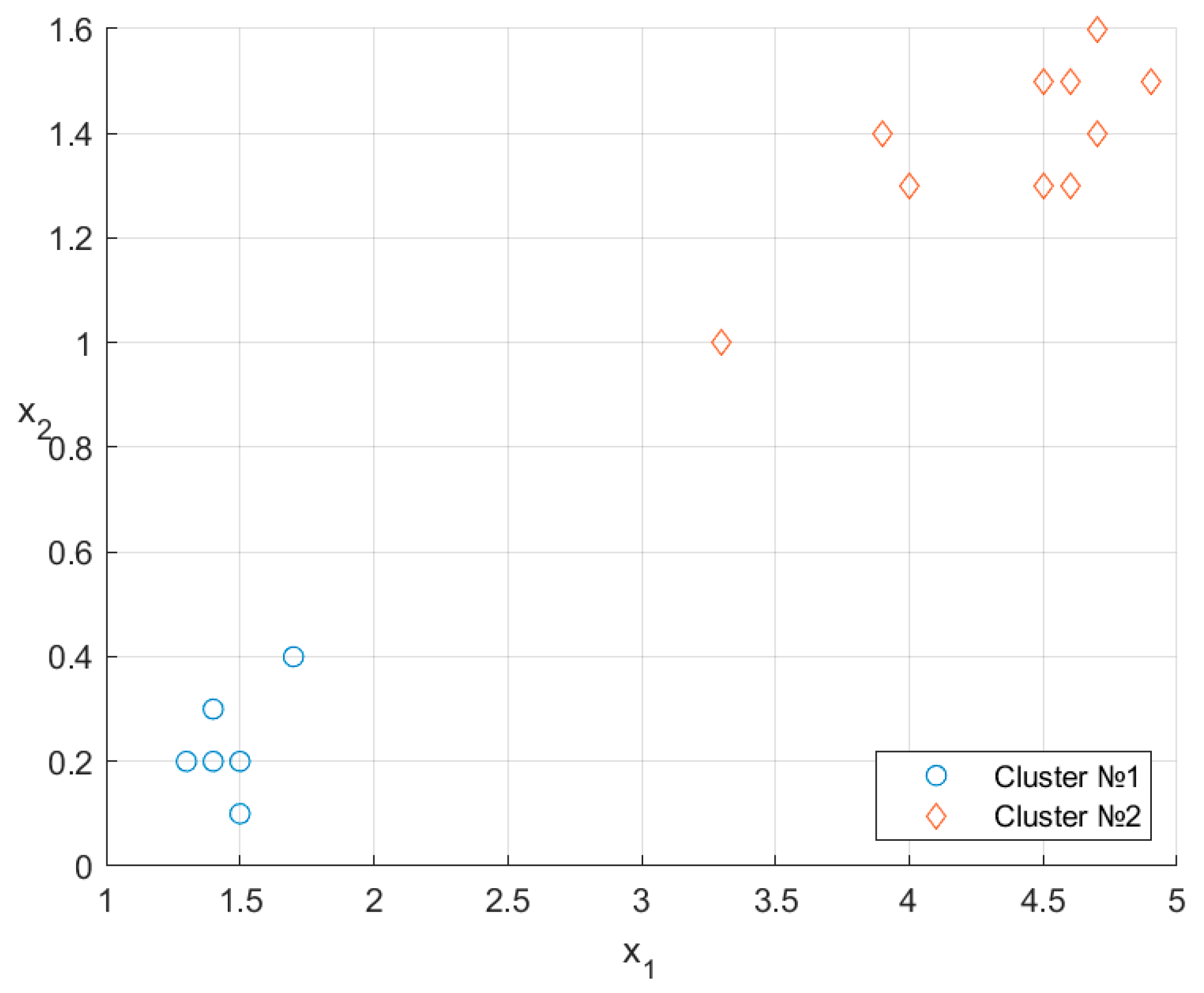
Figure 1 shows the arrangement of the data points on the plane.

First, we apply the algorithm $R2K\left(10\right);$ see Section 5.1.

The minimum and maximum elements are

$$inf\left(D_{(20\times 20)}\right)=0,sup\left(D_{(20\times 20)}\right)=3.73.$$

(38)

The data matrix indicator is $disX=1.7382.$ Let $\epsilon =0.15$.

The ensemble of possible clusters has the size $K\left(10\right)=184786$. The cluster with number $k=256$ has the form $i_1=1,i_2=2,i_3=3,i_4=4,i_5=5,i_6=6,i_7=7,i_8=14,$$i_9=15,i_{10}=20$. The distance matrix $D_{\left(10\right)}^{\left(256\right)}$ is presented in

Table 2. Distance matrix for cluster $\mathcal{K}\left(256\right)$.

No.	1	2	3	4	5	6	7	8	9	10
1	0	0.1	0.22	3.01	3.45	3.32	3.27	3.36	3.36	3.36
2	0.1	0	0.14	3.1	3.55	3.42	3.36	3.45	3.45	3.45
3	0.22	0.14	0	3.16	3.61	3.48	3.42	3.51	3.51	3.51
4	3.01	3.1	3.16	0	0.45	0.32	0.28	0.36	0.36	0.36
5	3.45	3.55	3.61	0.45	0	0.14	0.2	0.1	0.1	0.1
6	3.32	3.42	3.48	0.32	0.14	0	0.14	0.1	0.1	0.1
7	3.27	3.36	3.42	0.28	0.2	0.14	0	0.1	0.1	0.1
8	3.36	3.45	3.51	0.36	0.1	0.1	0.1	0	0	0
9	3.36	3.45	3.51	0.36	0.1	0.1	0.1	0	0	0
10	3.36	3.45	3.51	0.36	0.1	0.1	0.1	0	0	0

.

The indicator of the matrix $X_{\left(10\right)}^{\left(256\right)}$ corresponding to the cluster ${\mathcal{K}}_{\left(10\right)}^{\left(256\right)}$ is

$$dis(X_{\left(10\right)}^{\left(256\right)})=1.5021.$$

(39)

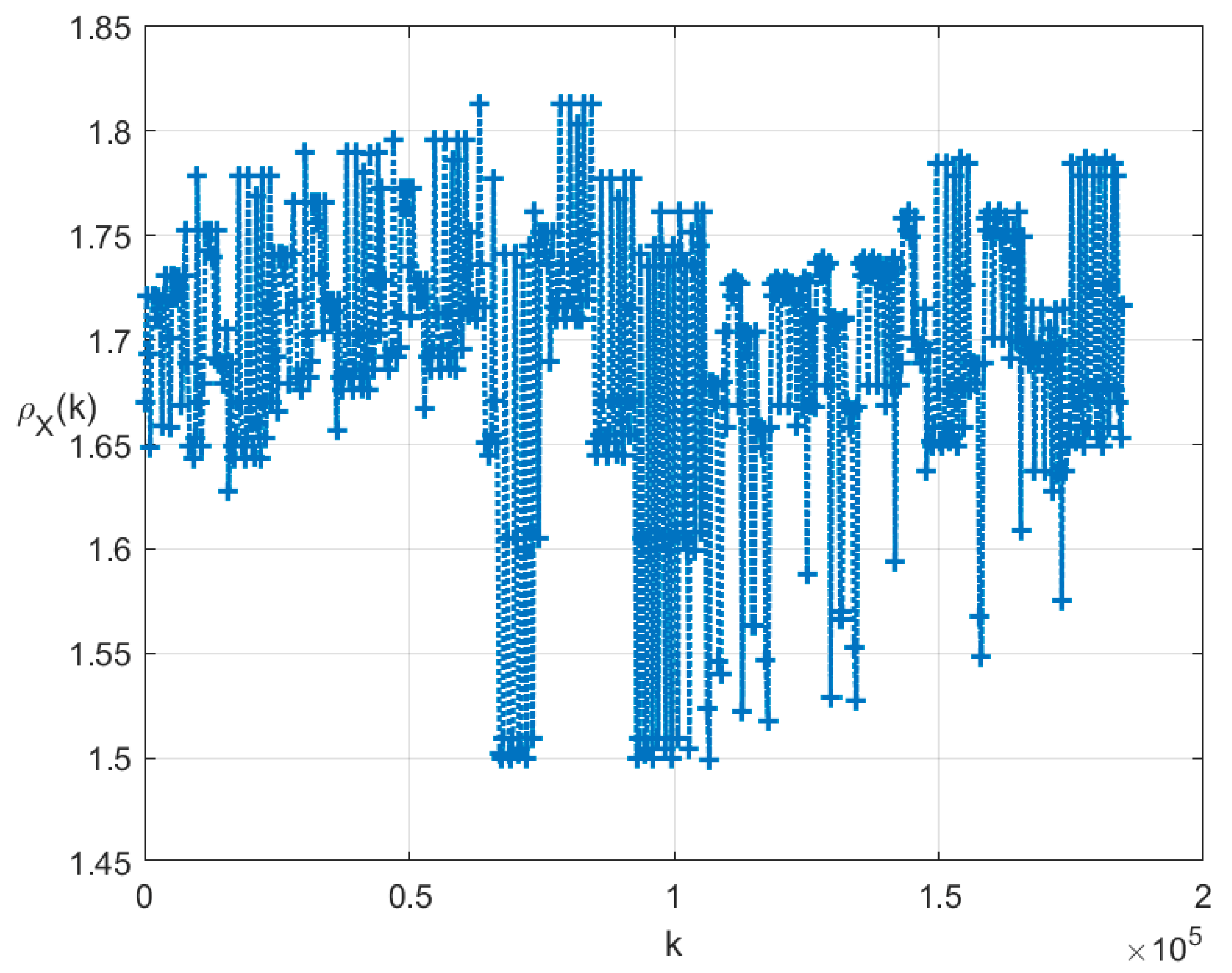
The indicators for the clusters $k=1,\dots ,184786$ are shown in Figure 2.

The entropy-optimal probability distribution for $s=10$ has the form

$$p^{*}\left(k\right|10)=\frac{exp(-{\lambda }^{*}dis(X_{\left(10\right)}^{\left(k\right)}))}{1+exp(-{\lambda }^{*}dis(X_{\left(10\right)}^{\left(k\right)}))},{\lambda }^{*}=12.1153.$$

(40)

The cluster ${\mathcal{K}}_1$ with the maximum probability is numbered by

$$k^{*}=166922,{\mathcal{K}}_1=\{4,5,6,7,11,14,15,16,17,20\},dis{\mathcal{K}}_1=0.1354.$$

(41)

The cluster ${\mathcal{K}}_2$ consists of the following data points: $\{1,2,3,8,9,10,12,13,18,19\}$.

The arrangement of the clusters ${\mathcal{K}}_1$ and ${\mathcal{K}}_2$ is shown in Figure 3.

A direct comparison with Figure 1 indicates a perfect match of 10/10: no clustering errors.

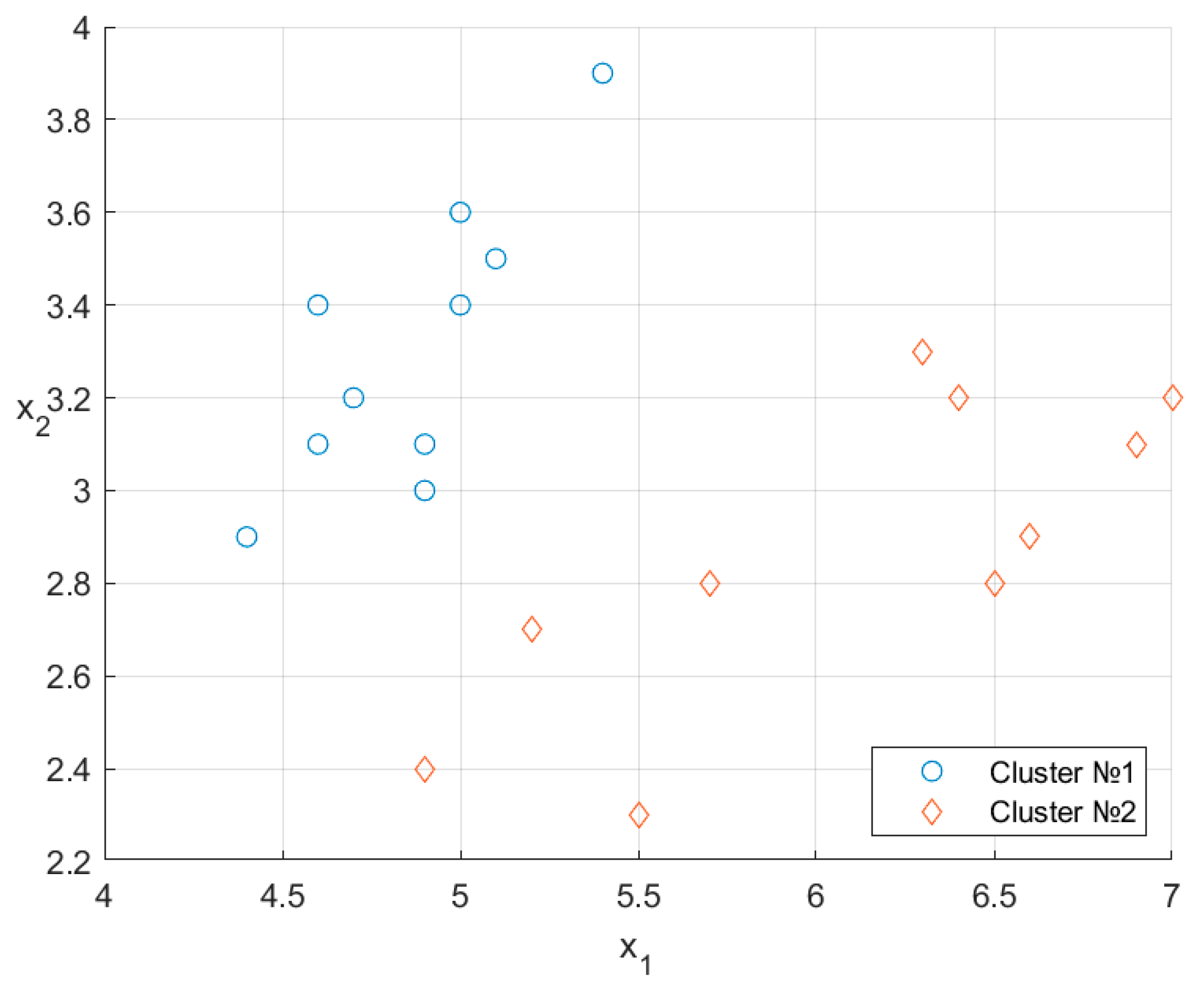
Example 2.

Consider another data matrix from the same dataset (

Table 3. Data matrix.

No.	${\mathit{x}}_1$	${\mathit{x}}_2$	Type
1	6.4	3.2	2
2	6.5	2.8	2
3	7.0	3.2	2
4	5.4	3.9	1
5	4.7	3.2	1
6	4.6	3.4	1
7	4.6	3.1	1
8	5.2	2.7	2
9	5.7	2.8	2
10	6.6	2.9	2
11	5.1	3.5	1
12	6.3	3.3	2
13	5.5	2.3	2
14	4.4	2.9	1
15	4.9	3.0	1
16	5.0	3.4	1
17	4.9	3.1	1
18	6.9	3.1	2
19	4.9	2.4	2
20	5.0	3.6	1

).

Figure 4 shows the arrangement of the data points.

Similar to Example 1, we apply the algorithm $R2K\left(10\right).$

We construct the distance matrix $D_{(20\times 20)}$ and find the minimum and maximum elements:

$$inf\left(D_{(20\times 20)}\right)=0,sup\left(D_{(20\times 20)}\right)=3.73.$$

(42)

Let $\epsilon =0.15$.

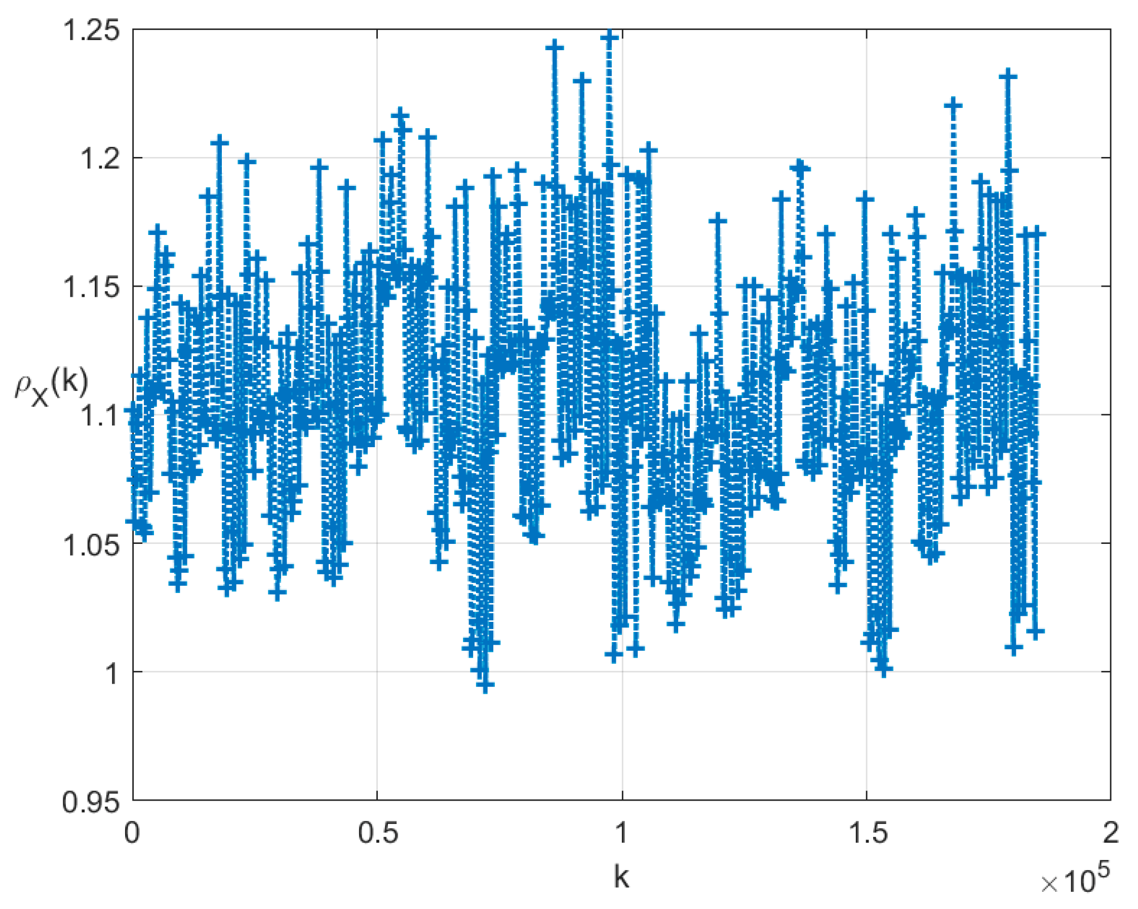
The ensemble of possible clusters has the size $K\left(10\right)=184786$. The indicators for the clusters $k=1,\dots ,184786$ are shown in Figure 5.

The entropy-optimal probability distribution for $s=10$ has the form

$$p^{*}\left(k\right|10)=\frac{exp(-{\lambda }^{*}dis(X_{\left(10\right)}^{\left(k\right)}))}{1+exp(-{\lambda }^{*}dis(X_{\left(10\right)}^{\left(k\right)}))},{\lambda }^{*}=100.$$

(43)

The cluster ${\mathcal{K}}_1$ with the maximum probability is numbered by

$$k^{*}=177570,{\mathcal{K}}_1=\{5,6,7,8,11,14,15,16,17,20\},dis{\mathcal{K}}_1=0.4420.$$

(44)

It consists of the following data points: $\{5,6,7,8,11,14,15,16,17,20\}.$ The cluster ${\mathcal{K}}_2$ consists of the following data points: $\{1,2,3,4,9,10,12,13,18,19\}.$

The arrangement of the clusters ${\mathcal{K}}_1$ and ${\mathcal{K}}_2$ is shown in Figure 6. A direct comparison with Figure 4 indicates a match of 8/10.

8. Discussion and Conclusions

This paper has developed a novel concept of clustering. Its fundamental difference from the conventional approaches is the generation of an ensemble of random clusters, accompanied by the matrices of inter-object distances averaged over the entire ensemble (the so-called indicators). Random clusters are parameterized by the number of objects s and their set $k\to \{i_1,\cdots ,i_s\}$. Therefore, the ensemble’s characteristic is the probability distribution of the clusters in the ensemble, which depends on s and k. A generalized variational principle of statistical mechanics has been proposed to find this distribution. It consists of the conditional maximization of the Boltzmann–Shannon entropy. Algorithms for solving the finite-dimensional and functional optimization problems have been developed.

An advantage of the novel randomized clustering method is complete algorithmization, independent of the properties of the clustered objects data. All existing clustering methods involve, more or less, various empirical techniques related to data properties.

However, this method requires high computational resources to form an ensemble of random clusters and their indicators.

References

- Mandel, I.D. Klasternyi Analiz (Cluster Analysis); Finansy i Statistika: Moscow, Russia, 1988. [Google Scholar]
- Zagoruiko, N.G. Kognitivnyi Analiz Dannykh (Cognitive Data Analysis); GEO: Novosibirsk, Russia, 2012. [Google Scholar]
- Zagoruiko, N.G.; Barakhnin, V.B.; Borisova, I.A.; Tkachev, D.A. Clusterization of Text Documents from the Database of Publications Using FRiS-Tax Algorithm. Comput. Technol. 2013, 18, 62–74. [Google Scholar]
- Jain, A.; Murty, M.; Flynn, P. Data Clustering: A Review. ACM Comput. Surv. 1990, 31, 264–323. [Google Scholar] [CrossRef]
- Vorontsov, K.V. Lektsii po Algoritmam Klasterizatsii i Mnogomernomu Shkalirovaniyu (Lectures on Clustering Algorithms and Multidimensional Scaling); Moscow State University: Moscow, Russia, 2007. [Google Scholar]
- Lescovec, J.; Rajaraman, A.; Ullman, J. Mining of Massive Datasets; Cambridge University Press: Cambridge, UK, 2014. [Google Scholar]
- Deerwester, S.; Dumias, S.T.; Furnas, G.W.; Landauer, T.K.; Harshman, R. Indexing by Latent Semantic Analysis. J. Am. Soc. Inf. Sci. 1999, 41, 391–407. [Google Scholar] [CrossRef]
- Zamir, O.E. Clustering Web Documents: A Phrase-Based Method for Grouping Search Engine Results. Ph.D. Thesis, The Univeristy of Washington, Seattle, WA, USA, 1999. [Google Scholar]
- Cao, G.; Song, D.; Bruza, P. Suffix-Tree Clustering on Post-retrieval Documents Information; The Univeristy of Queensland: Brisbane, QLD, Australia, 2003. [Google Scholar]
- Huang, D.; Wang, C.D.; Lai, J.H.; Kwoh, C.K. Toward multidiversified ensemble clustering of high-dimensional data: From subspaces to metrics and beyond. IEEE Trans. Cybern. 2021. [Google Scholar] [CrossRef] [PubMed]
- Khan, I.; Luo, Z.; Shaikh, A.K.; Hedjam, R. Ensemble clustering using extended fuzzy k-means for cancer data analysis. Expert Syst. Appl. 2021, 172, 114622. [Google Scholar] [CrossRef]
- Jain, A.; Dubs, R. Clustering Methods and Algorithms; Prentice-Hall: Hoboken, NJ, USA, 1988. [Google Scholar]
- Pal, N.R.; Biswas, J. Cluster Validation Using Graph Theoretic Concept. Pattern Recognit. 1997, 30, 847–857. [Google Scholar] [CrossRef]
- Halkidi, M.; Batistakis, Y.; Vazirgiannis, M. On Clustering Validation Techniques. J. Intell. Inf. Syst. 2001, 17, 107–145. [Google Scholar] [CrossRef]
- Han, J.; Kamber, M.; Pei, J. Data Mining Concept and Techniques; Morgan Kaufmann Publishers: Burlington, MA, USA, 2012. [Google Scholar]
- Popkov, Y.S. Randomization and Entropy in Machine Learning and Data Processing. Dokl. Math. 2022, 105, 135–157. [Google Scholar] [CrossRef]
- Popkov, Y.S.; Dubnov, Y.A.; Popkov, A.Y. Introduction to the Theory of Randomized Machine Learning. In Learning Systems: From Theory to Practice; Sgurev, V., Piuri, V., Jotsov, V., Eds.; Springer International Publishing: Cham, Switzerland, 2018; pp. 199–220. [Google Scholar] [CrossRef]
- Popkov, Y.S. Macrosystems Theory and Its Applications (Lecture Notes in Control and Information Sciences Vol 203); Springer: Berlin, Germany, 1995. [Google Scholar]
- Popkov, Y.S. Multiplicative Methods for Entropy Programming Problems and their Applications. In Proceedings of the 2010 IEEE International Conference on Industrial Engineering and Engineering Management, Xiamen, China, 29–31 October 2010; pp. 1358–1362. [Google Scholar] [CrossRef]
- Polyak, B.T. Introduction to Optimization; Optimization Software: New York, NY, USA, 1987. [Google Scholar]
- Joffe, A.D.; Tihomirov, A.M. Teoriya Ekstremalnykh Zadach (Theory of Extreme Problems); Nauka: Moscow, Russia, 1974. [Google Scholar]
- Tihomirov, V.M.; Alekseev, V.N.; Fomin, S.V. Optimal Control; Nauka: Moscow, Russia, 1979. [Google Scholar]
- Popkov, Y.; Popkov, A. New methods of entropy-robust estimation for randomized models under limited data. Entropy 2014, 16, 675–698. [Google Scholar] [CrossRef] [Green Version]
Figure 1.
Data points on the two-dimensional plane.
Figure 2.
Indicators for .
Figure 3.
Randomized clustering results.
Figure 4.
Figure 5.
Figure 6.