
Assessment of CNN-Based Models for Odometry Estimation Methods with LiDAR


University Institute for Automobile Research (INSIA), Campus Sur UPM, Universidad Politécnica de Madrid (UPM), 28031 Madrid, Spain
*
Author to whom correspondence should be addressed.
Mathematics 2022, 10(18), 3234; https://doi.org/10.3390/math10183234
Submission received: 15 July 2022
/
Revised: 30 August 2022
/
Accepted: 2 September 2022
/
Published: 6 September 2022
(This article belongs to the Special Issue Numerical and Machine Learning Methods for Applied Sciences)
Abstract
:The problem of simultaneous localization and mapping (SLAM) in mobile robotics currently remains a crucial issue to ensure the safety of autonomous vehicles’ navigation. One approach addressing the SLAM problem and odometry estimation has been through perception sensors, leading to V-SLAM and visual odometry solutions. Furthermore, for these purposes, computer vision approaches are quite widespread, but LiDAR is a more reliable technology for obstacles detection and its application could be broadened. However, in most cases, definitive results are not achieved, or they suffer from a high computational load that limits their operation in real time. Deep Learning techniques have proven their validity in many different fields, one of them being the perception of the environment of autonomous vehicles. This paper proposes an approach to address the estimation of the ego-vehicle positioning from 3D LiDAR data, taking advantage of the capabilities of a system based on Machine Learning models, analyzing possible limitations. Models have been used with two real datasets. Results provide the conclusion that CNN-based odometry could guarantee local consistency, whereas it loses accuracy due to cumulative errors in the evaluation of the global trajectory, so global consistency is not guaranteed.
1. Introduction
Vehicle positioning is a key aspect for autonomous driving, for which several traditional solutions, such as satellite positioning and inertial systems, are being applied. On the other hand, the perception of the environment is essential for safe navigation, and LiDAR is one of the most reliable elements for detecting obstacles and free areas. From the use of these sensors in vehicles, visual odometry (VO) has become relevant as an estimation of the relative movement between consecutive observations, ensuring local consistency, although it would not be possible to achieve a global optimization in real time, as it occurs when trajectory closure techniques are applied that minimize the generated drift error [1]. Despite this, VO techniques have several advantages, including a longer reliable estimation time compared to other location systems, and their implementation versatility. For this reason, they have been applied in mobile robotics, from space missions to Mars [2], and in ground vehicles in outdoor environments using artificial vision [3]. On the other hand, 3D LiDAR sensors can provide precise information about the environment that can be useful for calculating positioning through VO or SLAM (simultaneous localization and mapping) algorithms. Thus, several developments based on this technology, such as V-LOAM [4], IMLS-SLAM [5], and MC2SLAM [6], stand out in the first positions of the KITTI odometry ranking [7]. Another example could be found in [8], which presents a fast 3D-pose-based SLAM system that estimates a vehicle’s trajectory by registering sets of planar surface segments, extracted from a 360° field of view, and image-based techniques are used for maintaining a low computational load.
On the other hand, among the tools for interpreting the environment, Deep Learning techniques are proving to be capable of solving a wide variety of complex problems. Among them, it is worth highlighting the applications for autonomous vehicles, such as for the semantic segmentation of the environment, obstacle detection, calculation of the driving strategy, or decision-making. However, it is not always advisable to apply this approach to provide a solution to any problem, only in those cases where the conditioning of the problem allows it. In this sense, Machine Learning provides suitable tools, when the solution requires too much manual adjustment, or is useful for complex problems, where a traditional approach fails to provide a definitive solution. Its application is also appropriate in changing environments, in which a generalization of operation is necessary.
Machine Learning models based on convolutional neural networks (CNNs) have demonstrated their effectiveness in vision-based obstacle detection. This technique is widely used for image recognition or semantic segmentation, due to its potential and effectiveness demonstrated in various applications in this field. Thus, CNNs have partially or totally solved some of the problems posed, especially regarding object detection [9].
However, these networks do not have to be used exclusively in classification or segmentation applications, as they can also be used in regression problems. In this case, the network output is a continuous signal, and, therefore, it is possible to study its viability to be used as a method of visual odometry, by estimating the values of translation and relative rotation. In this sense, several developments have tried to study this feasibility, as in [10], using stereo vision for feature extraction, as well as the estimation of discrete values, the approach of [11] using a LiDAR sensor, or the development of [12], using computer vision and the combination of convolution and recurrent networks (RNNs). Ref. [13] also uses a convolutional neural network, based on computer vision, to calculate the trajectory to be followed by an automated guided vehicle. Other approaches look for data fusion from several sensors. An example is [14], in which fuzzy fusion of stereo vision, an odometer, and GPS is applied to reduce the error in the absolute location of autonomous vehicles. In this case, the results do not rely only on computer vision, so they are not comparable with pure VO methods. Ref. [15] shows a review of the use of Deep Learning in Loop Closure Detection for solving the SLAM problem. Among different techniques, CNNs probe their good performance for this task. In this case, both computer vision and LiDAR are cited, but the former are a more widespread solution (e.g., [16]).
On the other hand, these AI techniques have some limitations. Specifically, those based on Deep Learning require a large amount of data to model the problem. Moreover, the use of these algorithms leads to a loss of internal understanding of the problem solving. To avoid this black box phenomenon, there are recent studies that try to establish guidelines to reach an interpretation of the internal process of these algorithms [17]. Therefore, one of the basic objectives of Machine Learning is to find models that allow us to conceptualize, predict, generalize, and learn from real behavior.
In this paper, the feasibility of implementing CNN models, for the estimation of vehicle odometry using a 3D LiDAR sensor as the only input information from an autonomous vehicle moving in real urban and interurban scenarios, is studied. One of the main contributions focuses on the study of the conditioning of the problem to address it through a Deep Learning approach and the study of the limitations, in terms of accuracy, that could be achieved with these models. In this way, the main objective is to develop a visual odometry methodology based on Machine Learning models centered on LiDAR technology, which is showing its usefulness and robustness for autonomous driving, but this is less often introduced for odometry problems than for computer vison. Then, from the point clouds obtained, the aim is to infer the speed and yaw of the vehicle to estimate its trajectory.
The rest of the sections are organized around the basic concepts necessary to define a model: data, parameters, and optimization. Firstly, Section 2 presents the whole method and tests with different datasets. The first step described in Section 3 focuses on the analysis of the available data that serves as the input to the model. Different configurations of representation of the environment are proposed to evaluate which is the most appropriate to achieve a better network performance. In Section 4, the suitability of CNNs as a tool for odometry estimation in a controlled scenario is assessed. For this purpose, a self-built dataset is used. To find a reference of the estimation accuracy with CNNs, their performance is compared with different multilayer perceptron (MLP) topologies, as they are widely known. Tests have been implemented with an instrumented vehicle in real situations. Finally, the study focuses on the determination of the final network topology and performance assessment. For this, in Section 5, the conclusions reached previously are applied to a reference dataset established as a worldwide benchmark.
2. Methods
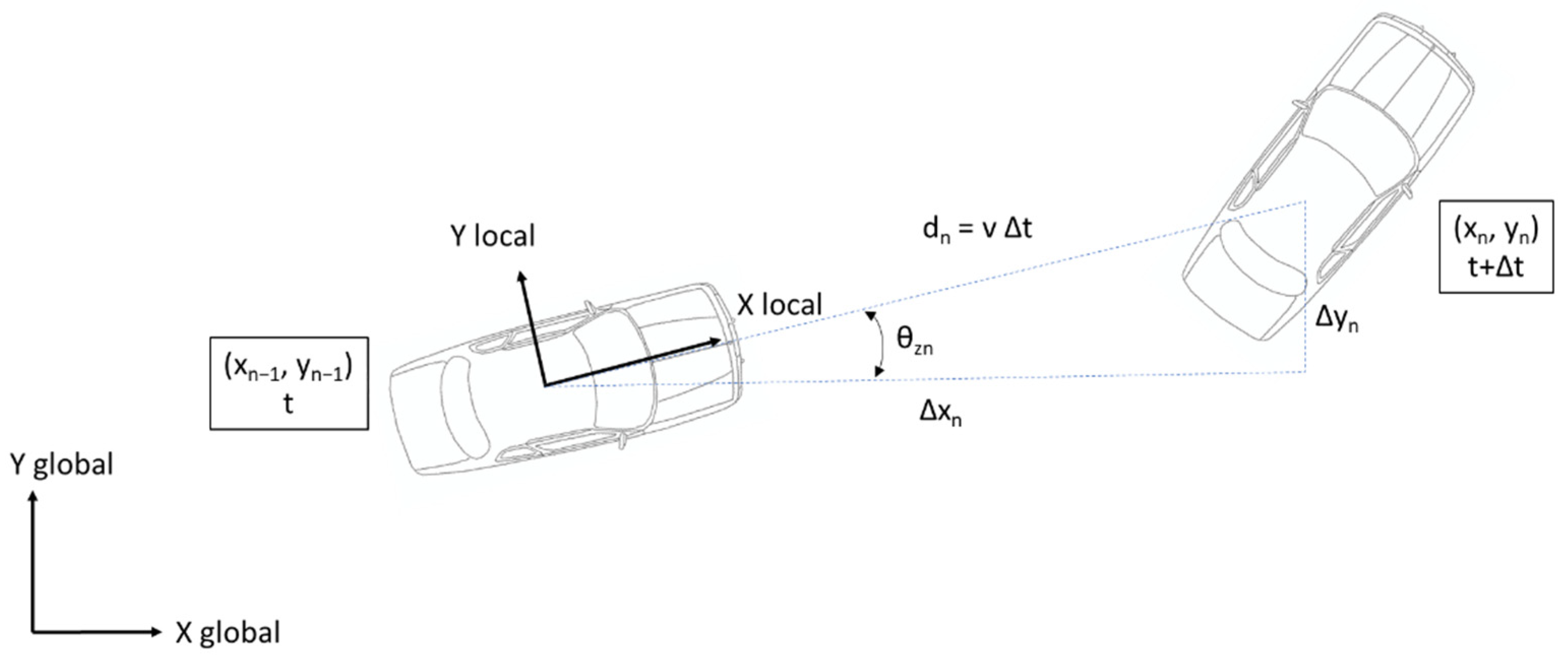
Positioning through VO implies the estimation of vehicle kinematic variables such as speed and yaw angle, similarly to what is done with inertial sensors. Then, considering Figure 1, the trajectory of the vehicle can be defined in Cartesian coordinates as follows [18]:
where () are the Cartesian co-ordinates, v is the cruising speed, Δt is the time between the two timestamps, and θz is the vehicle yaw angle.
The aforementioned coordinates (, ) can be considered to describe the relative motion between two time instants at time , and they also denote the position of the vehicle . Therefore, a finite sequence of steps is given by Equations (3) and (4):
The SLAM problem definition defines as the true map of the environment. This is defined by the landmarks and patterns extracted at each instant. Similarly, a measurement of the environment, , is acquired from the sensor used. This is the total sequence of measurements, as defined in Equation (5):
Therefore, the general definition of SLAM is to estimate the position of the vehicle and the map of the environment from observable variables. In a probabilistic way, it is given by Equation (6):
This involves solving two models. One model relates odometry to position and another model relates the measurements to the environment and the position . When it comes to odometry estimation, only the first model, Equation (7), is addressed:
This paper focuses on analyzing the feasibility of CNN topologies to obtain a consistent estimation of the transitions . Specifically, to obtain each , it is necessary to apply a mapping from input to output variables, as defined in Equation (8). These input variables will be two consecutive frames in the point cloud domain . The transitions parameters are (, ).
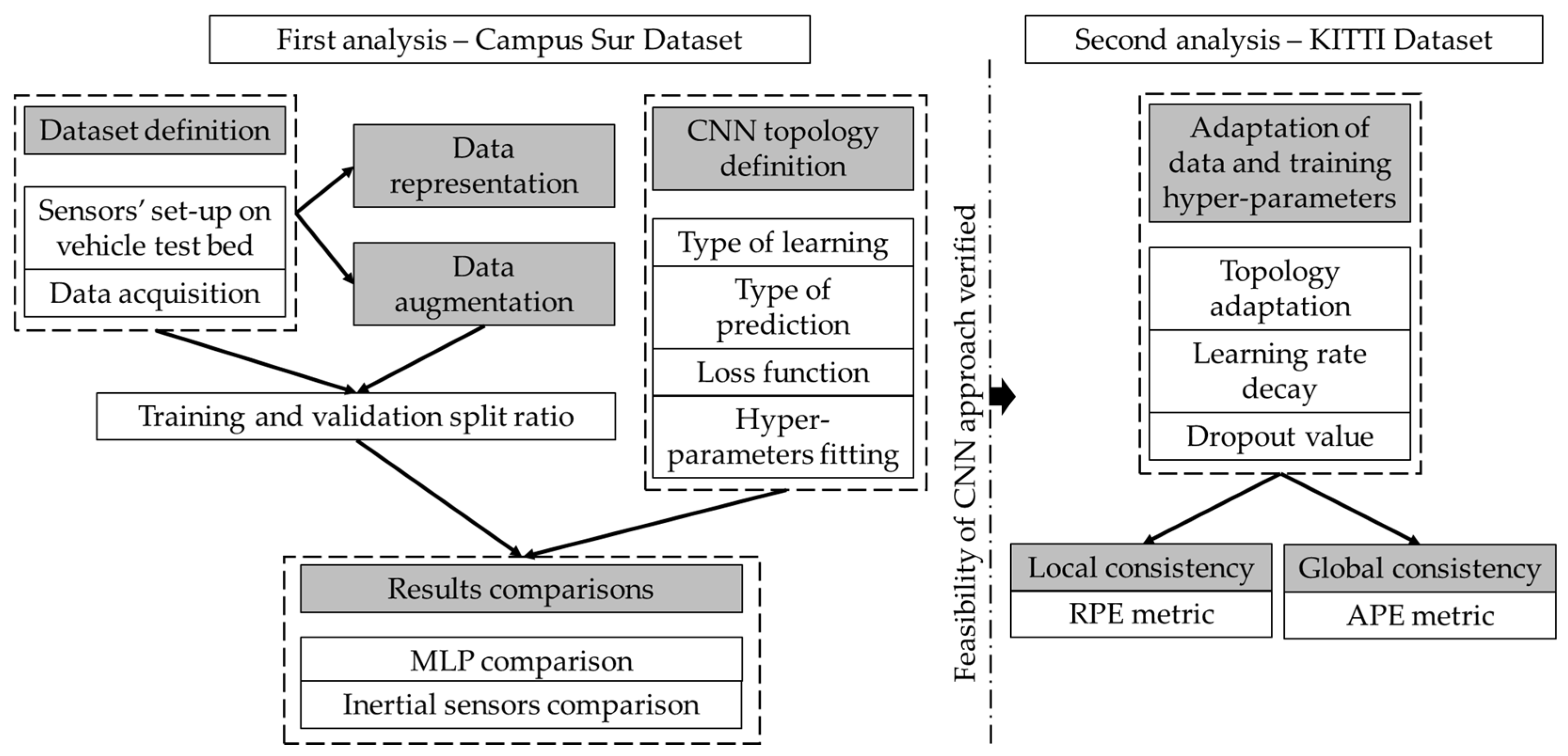
In order to fulfill the objective proposed in the paper, two main interrelated approaches are addressed, as shown in Figure 2.
The first analysis seeks to evaluate the feasibility of using CNN as an inference method for the vehicle’s odometry. Different topologies of Machine Learning models are compared to study their adequacy to the problem. The results, up to this point, are also compared with those obtained with inertial sensors. In a more in-depth study of best fit, different alternatives are evaluated with respect to data preprocessing, augmentation technics, and model parameter fitting. Within the first analysis, tests have been carried out on a self-developed dataset: Campus Sur.
In the second approach, once the feasibility of the CNNs has been verified, the aim is to obtain a more refined and robust result. For this, the adjustment of the hyper-parameters and network topology is addressed, this time, using a reference dataset: KITTI. The influence in estimation performance and accuracy is tackled in this case.
Both data from real tests in real roads and streets with an instrumented vehicle and the use of widespread datasets are considered for model fitting and assessing. Finally, the assessment of the feasibility of using this method for results global and local consistency is presented. It must be noticed that the use of real data obtained from a vehicle provides the opportunity of exploring the potential of the proposed tools under predefined conditions. Moreover, in order to analyze the generalization of the method to other environments, it is proposed the use of another large and reference dataset to consolidate the results.
Using a 3D LiDAR sensor is a challenging scenario because point clouds are not as finely detailed as images in terms of density and do not always provide sufficient features for matching. Additionally, point cloud matching generally requires high processing power, so it is necessary to optimize the processes to improve speed.
A fundamental aspect of the paper’s contributions is the selection of CNN models to solve the odometry problem. Thus, the design of a generic convolution neural network is aimed at taking advantage of the spatial structure of an image. The value of a pixel is usually related to the pixels that surround it and, therefore, provides valuable information to extract characteristic patterns. On the other hand, conventional networks such as MLP do not take this spatial arrangement into account. This means that CNNs can be successfully applied in the case of processing images that have been generated from LiDAR data. Moreover, the comparison with MLP is of interest since these models are widely known to establish a baseline in the analysis.
By using a Deep Learning based approach, the training phase of the models becomes an optimization problem, where the error between the estimation of the model itself and the true values is minimized. In the case of the Campus Sur dataset, the true values have been acquired from the sensors on board the test vehicle, while, in the KITTI dataset, a ground truth is provided. Specifically, the implemented loss function is the Root Mean Square Error (RMSE), as given by Equation (9).
where are the observed values, are the values predicted by the network, and is the number of observations. It should be noted that, although the selection of RMSE as loss function during the model optimization process is correct, this metric does not represent the accuracy of the trajectory reconstruction from the integration of the odometry data. The error measured as RMSE is efficient in error optimization but is indicative of the error made with respect to the reference signal. This reference signal, depending on the acquisition mode or data preprocessing, may differ when using one data set or another and, therefore, results cannot be extrapolated. The training and validation results presented in this paper are carried out under the same hardware and software. A GNU/Linux machine with Intel Xeon CPU E3-1200 (family) v3/4th Gen, NVIDIA GeForce GTX 980 Ti with 2816 CUDA cores, and 6GB of RAM has been used. It was programmed using Python3, TensorFlow, and Keras 2, thus managing to benefit from the use of GPUs.
3. Data Selection and Processing
Since 3D LiDAR sensors provide a three-dimensional points cloud from the environment in which the points contain the cartesian coordinates and reflectivity, it can be stated that these sensors work in the spatial domain. As odometry estimation is a geometrical problem, the initial 3D LiDAR data fits as a good starting point to address the calculation of relative translation and rotation of the motion.
The proposed method is based on Deep Learning models, so to define them and establish the learning process, it is necessary to know the data typology and the preprocessing steps. This data processing is necessary to adjust the networks input that will infer the relative motion between two consecutive observations.
3.1. Input and Output Data
The point clouds are transformed to a matrix domain. A data matrix is created for each observation (frame) and then stacked one behind the other, resulting in a multidimensional matrix containing the spatial information of consecutive frames.
The size of these matrices is H × W × C, where H and W are the height and width dimensions, respectively, corresponding to the resolution of the data matrix; and C is the sum of the number of channels used by each one.
The output data of the model is the linear vehicle velocity and yaw rate between the two consecutive frames.
3.2. Description of the Datasets
Two different datasets have been used for the learning process. On the one hand, a dataset generated with an instrumented vehicle available at the University Institute for Automobile Research of Technical University of Madrid (INSIA-UPM), with the main purpose of obtaining preliminary results and validating the suitability of CNNs for solving the problem, is used. Specific scenarios are looked for, to have a clear idea of how the method could infer vehicle motion and distinguish performance, whether the scenario in training and on a test coincide or not. On the other hand, the KITTI dataset, available from the Karlsruhe Institute of Technology (KIT), is used, with a different LiDAR model and sensors that provide an accurate ground truth. The aim in the latter case is to achieve more refined results, as it is a more complete dataset that serves as a benchmark for many researchers.
A common aspect in both datasets is the split between training and validation sets. Due to the type of problem to be solved, there is a time dependence between observations, so it is not possible to randomly shuffle the whole dataset. In this sense, to ensure that there are temporally related data in the training and validation sets, complete sequences are reserved. They represent a 90–10% ratio of the total data, respectively. Once this partitioning is done, the training set is randomly unsorted to feed the data to the input layer, while the validation set is not, so that the network inference on this set is obtained in a time-ordered way, according to the sequence.
3.3. Data Representation
For a better understanding of the conditioning of the problem, different data preprocessing alternatives are evaluated to select the one that best suits the problem. Three types of data maps have been defined: Depth Maps, Coordinate Maps, and Grid-occupancy Maps. All data maps described below normalize a fixed threshold of distance (0–25 m) from 0 to 1. For this reason, no information is lost in the scaling, which would be the case if the maximum and minimum values of each frame were normalized separately.
- Depth Maps:
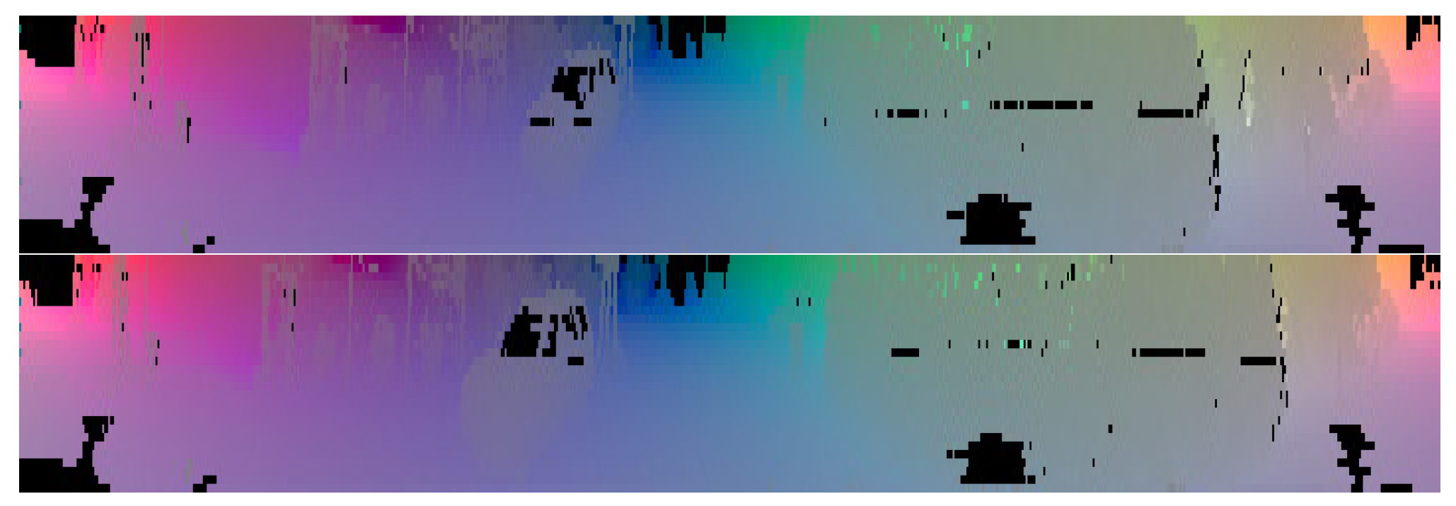
The distance data is projected onto a two-dimensional matrix. The horizontal axis corresponds to the horizontal angle or azimuth values of the points, covering a horizontal field of view of 360°. The vertical axis corresponds to each of the laser layers. In the case that several points are obtained in the same cell, i.e., they are in the same horizontal and vertical resolution range of the matrix, the closest distance data prevails because this data would be more representative of the movement.
The data images created are stacked in pairs corresponding to two consecutive timestamps, obtaining a matrix of dimensions Hd × Wd × 2. Figure 3 shows an example of the data matrix pairs with the described configuration.
Due to the divergence between LiDAR points, some cells have not available data for certain angular resolutions. If the map resolution is low, the number of invalid values is relevant for the learning process. This could be mitigated by performing a linear interpolation between horizontally adjacent pixels. This would result in a dense data image with the original resolution.
On the other hand, the point density is inversely proportional to the square of the distance. Therefore, the distribution of the pixel values of the images is not balanced. To compensate this distribution and to obtain a histogram of values uniformly distributed over the whole range, logarithmic transformation is applied as a scaling function. This logarithmic function improves the contrast between similar values, highlighting the characteristics from which patterns can be extracted.
- Coordinate Maps:
Similar to the Depth Maps, a data matrix is generated, this time from the (X, Y, Z) coordinates of the LiDAR points. The motivation of this data configuration is based on the hypothesis of a better geometrical conditioning of the problem. By including the coordinate information separately in the input matrix, inference of linear displacements and rotation could be improved through the variation of coordinates and not distances, as in the previous case.
The difference from the process of generating Depth Maps lies in the fact that, in this case, each matrix contains three channels of information, i.e., one channel for each coordinate individually. Therefore, a data map is obtained, where each cell contains the X coordinates in the first channel, the Y coordinates in the second channel, and the Z coordinates in the third channel. Moreover, during the generation of this map type, interpolation between horizontally adjacent values would be considered, due to the absence of information in certain pixels. When stacking two data maps of this type, the input matrix has a resolution of Hc × Wc × 6. An example of such Coordinate Maps can be seen in Figure 4.
- Grid-occupancy Maps:
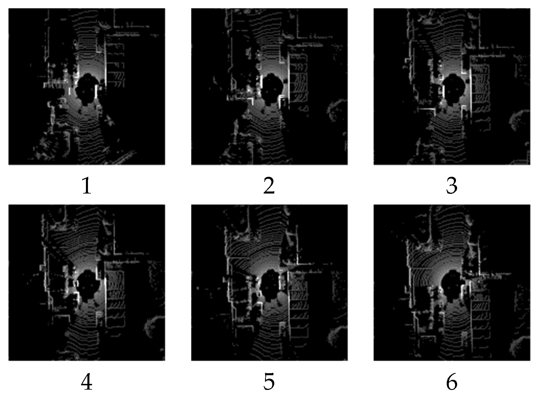
These maps consist of a bird’s eye view of the vehicle environment of a delimited area divided into grids. Each grid corresponds to a cell of the data matrix containing the value of the number of points that have been obtained at the distance corresponding to the grid. Therefore, the greater the number of points obtained in a grid is, the greater the numerical value of the grid.
In the projection on the X–Y plane, it can be seen how the main elements of the environment, i.e., those on which a greater number of points have been obtained, move around the LiDAR. This representation is the most intuitive one, as the movement between observations can be noticed, which indicates a possible advantage for the learning process. The generated maps have a resolution of Hg × Hg × 1 (Figure 5). Finally, when the maps of two consecutive observations are stacked, the input matrix size is Hg × Hg × 2.
Some other alternatives have been considered such as using the reflectivity information or including three consecutive frames, t, t − 1, and t − 2, or wider intervals between timestamps, but improvements were not detected, so they were discarded.
3.4. Data Augmentation
For a correct training that allows the model to generalize correctly, a large amount of data is necessary. There are different methods to increase the number of training data known as data augmentation techniques. These techniques are mainly used when the problem is complex or when there is not enough data available, thus avoiding overfitting problems. In this case, two techniques have been implemented, the first one called “Mirroring” and the other one called “Shaking” [19].
“Mirroring” doubles the number of observations when calculating the inverse image. It is based on flipping the images 180° and, in the same way, calculating the inverse path of the new environment to be used as ground truth.
In the so-called “Shaking” technique, the LiDAR uncertainty itself is used to generate clouds of similar points. Considering that these sensors usually have an accuracy of ±3 cm, each point could be randomly placed in a sphere of 3 cm radius. Therefore, clouds of similar points are generated by adding a noise to each point bounded by this threshold.
4. Preliminary Assessment of CNN as Odometry Tool
The problem nature needs to be deeply understood to be able to define the framework of the problem to be tackled.
- (1)
- Type of learning:
The problem is tackled as a supervised learning type, since the model fitting will be performed with a known positioning. The objective of this type of learning is to adjust the model parameters from a set of training data, so that the model could generalize an output when new cases are presented. Precisely, driving in both urban and interurban areas is characterized by highly changeable environments and, therefore, this ability to generalize is of great interest.
- (2)
- Type of prediction:
The model must infer the value of a continuous signal representing the relative translation and rotation of the vehicle between two observations. Therefore, the type of prediction is a regression of linear speed and yaw rate. This fulfills the principle of local consistency of odometry methods. Absolute positioning and cumulative yaw angle are not estimated. In addition, estimations of the two signals together by the same network (multivariate regression problem) and using a fitted model to estimate each signal individually (univariate regression problem) will be compared.
- (3)
- Measuring learning performance:
Another fundamental element during the optimization process is to define a loss function. Since the problem being addressed is a regression problem, the error is measured by calculating the RMSE. This error metric emphasizes major differences between the estimate and the true value. Other metrics considered, such as Mean Absolute Error (MAE), are not as sensitive to larger errors, so they are discarded.
4.1. Campus Sur-UPM Dataset
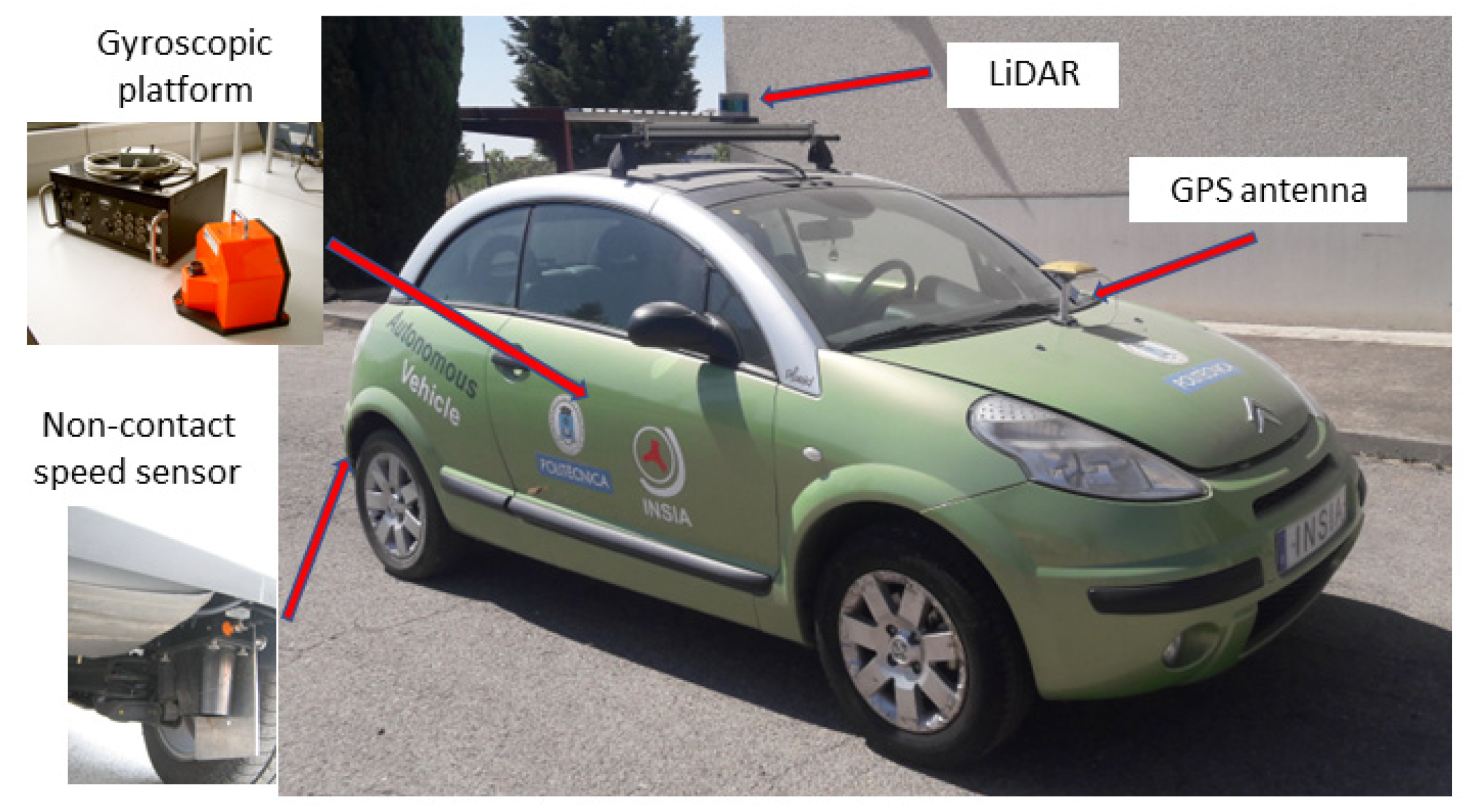
For preliminary results, the dataset used has been generated with the sensors installed in a testbed vehicle. The vehicle has the capability of being driven automatically or manually. A VLP-16 LiDAR sensor has been used to collect the environment information with a RTK DGPS Topcon GB-300 receiver, a high-resolution RMS FES 33 gyroscopic platform, and an L-CE Correvit non-contact speed sensor for the ground truth signal. It is worth mentioning that, although a gyroscope has been used, and, therefore, the signal may suffer from drift errors, the yaw rate signal is accurate, so this error only manifests itself when integrating over time. Furthermore, the satellite global positioning is only used for having a global ground truth, but it is not used in any calculation. Figure 6 shows the vehicle and the instrumentation.
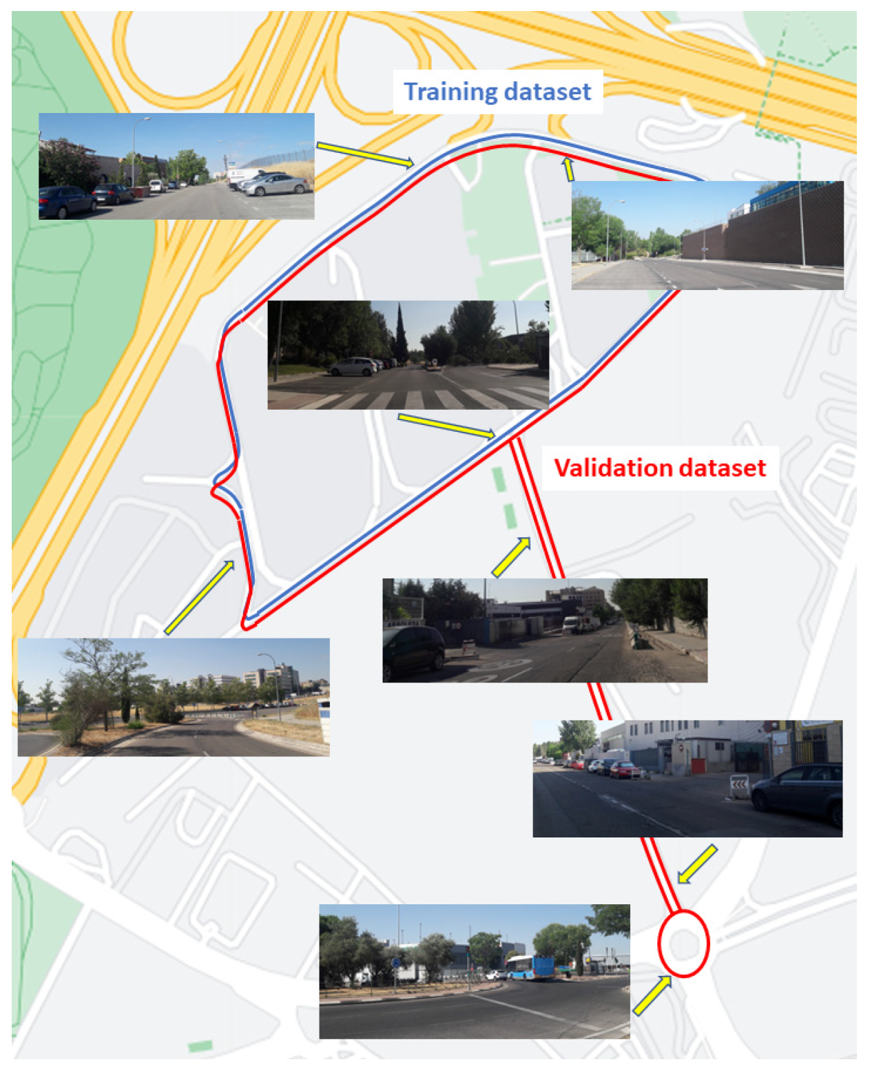
The training data set is made up of the data acquired during one hour driving in an urban environment located in the Campus Sur-UPM (Madrid, Spain) and surroundings, which is equivalent to 25.6 km (several laps have been done with different traffic and parking-space-occupancy scenarios). The data acquisition and synchronization rate has been 10 Hz. During data acquisition, the driver’s behavior is varied, so that different speeds, stops, or lane changes are included, favoring the generalization of the model. In addition, it mixes open environments with narrower streets and closed turns. As a result, the dataset contains a great diversity in the observations.
For the validation set, a different route has been chosen. It maintains the same initial and final stretches as the training set, but the intermediate section corresponds to an environment not included in the training set. In this way, it is intended to observe the suitability of the model for inferring odometry both in scenarios previously observed during training, as well as in completely new areas. The validation set comprises 2.85 km, equivalent to 4756 observations. Figure 7 shows the two trajectories, for training and validation phases. The most relevant difference between them is the fact of including a two-lane narrow street and a roundabout in the second one. This road elements imply vehicle maneuvers (turns and speed reductions to zero) that have not been considered in the other dataset, so it is considered a good test for assessing the CNN model’s generalization ability.
4.2. Hyper-Parameters Fitting
One of the most relevant factors during the learning process is the optimization algorithm used. In this case, the Adam optimizer [20] has been used in all tests, because it is a balanced algorithm in terms of precision and efficiency with respect to others such as SGD or RMSProp, although the latter can lead to better results if a fine-tuning of the other hyper-parameters is carried out [21].
It is also worth highlighting the interactions between hyper-parameters. In this sense, a mini-batch based method is selected as a way to compute the optimization. This strategy entails choosing a mini-batch size by which the model weights are computed and updated. This mini-batch size has a strong interrelation with the hyper-parameter of the learning rate. Therefore, depending on the topology evaluated, a balance between mini-batch size and learning rate is sought to result in training that is time-efficient and generalizes correctly.
To avoid model overfitting, dropout is used as a regularization method [22]. The selection of this hyper-parameter is studied according to its impact on the result.
4.3. Evaluated Architecture Alternatives
Once the problem has been defined, it is possible to assess the general characteristics of the models. Firstly, Depth Maps of the environment in two consecutive observations are used. These maps are expected to contain recognizable patterns, where CNNs perform well when extracting and using them to achieve a better fit.
To confirm the validity of the CNNs, their performance is compared with another well-known type of neural network model, such as the multilayer perceptron (MLP)-based models. This type of model is widely known and, therefore, defines a reference with respect to the performance obtained by CNNs applied to this problem. For the first assessment, six convolutional network topologies and two MLP topologies are compared using the Campus Sur-UPM dataset. Some hyper-parameters may vary according to the topology.
- Convolutional neural networks’ topologies:
In the case of CNNs, the architecture used can be divided into two blocks: a feature extraction block and a signal estimation block (Figure 8). The first block, focused on feature extraction, is composed of a set of layers where convolutions and space reductions are successively applied to make it possible to learn key patterns from the input data. Then, more general patterns, obtained in the last layers, are modified to a vector form and connected to the value estimation block. This block is defined as a fully connected topology, similar to that used in MLP models.
The optimization process is also carried out with Adam, and it has a selected learning rate of 10−3. For the regularization, a dropout of 0.4 and 0.1 has been applied after the fully connected layers. The convolution layers have several associated sublayers or operations that are normally considered as part of them: a Local Response Normalization layer (LRN) and a Max Pooling layer.
For nomenclature convenience, each convolution layer is specified as CH,W,N, with N filters of dimension H × W with the corresponding LRN layer. The Max Pooling layer is designated as PH,W for the MaxPool operation with H × W dimension filters. Finally, the term FCN describes the fully connected layers composed of N neurons. Table 1 shows the models and the results achieved. Note that topologies CNN-1 and CNN-4; CNN-2 and CNN-5; and CNN-3 and CNN-6 are equivalent pairwise, with respect to the layer structure, although their dropout value has been varied. There is a strong dependence on the global consistency when the dropout value is changed, since a small variation influences the RMSE value. Thus, a small deviation in the yaw rate estimation can lead to totally different results, due to the error accumulation when integrating this signal over time.
In addition, it can be observed that by increasing the network complexity (i.e., adding more convolutional layers) from CNN-1 to CNN-2 topologies (and, therefore, from CNN-4 to CNN-5), there is an improvement in the accuracy of the estimation of the two output variables. However, when the size of the network is increased further, these improvements are no longer significant, and the results even worsen. In the case of CNN-2 to CNN-3 topologies, the training results become worse, and in the case of going from CNN-5 to CNN-6, both training (only yaw rate) and validation results worsen. It has been observed that the error obtained is very sensitive to the small variations of the dropout hyper-parameter. On the other hand, increasing this value reduces the error in validation in most cases, but not in the errors obtained during training.
The different tests carried out indicate that the best topology is composed of three convolution layers and a dropout of 0.4 (CNN-5). The preliminary results with this architecture provide RMSE values of 2.905 km/h and 2.577°/s in speed and yaw rate, respectively. Although these errors could be considered small with respect to their reference signal, and local consistency is guaranteed, the trajectory integration results in a poor reconstruction, so a high global consistency is not reached. Figure 9 shows the estimation of this architecture on the two output variables, comparing the result with the ground truth.
As described above, the Campus Sur-UPM dataset shares the initial and final stretches of the trajectory in the training and validation sets. However, Figure 9 shows the ability of the model to generalize to unknown areas. In the estimates corresponding to the observations between instants 150 and 250 s, some residual linear speed or small deviations in the yaw rate are observed while the vehicle was stationary (0 km/h), mainly due to the dynamic environment where the test takes place. However, it is noteworthy that, in the training set of this dataset, no situation with the vehicle stationary was included, but the network can infer a speed close to zero.
- Multivariate regression versus univariate regression problem:
The possibility of training two independent models to estimate the speed and yaw rate is considered, thus becoming a univariate regression problem. Trajectory reconstruction results have shown that it is more dependent of errors in the yaw rate estimation than of the speed estimation, i.e., only deviations in speed estimations have an assumable impact on the trajectory. For this reason, the aim is to search for a model that specializes in optimizing the yaw rate error.
Keeping the topology and training conditions as in CNN-3, this time as a univariate model, an RMSE of 0.63°/s has been achieved during training, and 3.26°/s has been achieved in validation (compared to 1.29°/s and 2.71°/s). With a univariate CNN-5 network, 0.63°/s was obtained during training and 3.13°/s during validation (compared to 1.32°/s and 2.57°/s, respectively).
From these first results achieved on the yaw rate only, errors of the same order of magnitude as in the multivariable models are obtained. However, the training time is much shorter, requiring fewer iterations to get to these values. On the other hand, it should be noted that, from these iterations onwards, the validation error begins to rise, while the training error continues falling, which translates into an overfitting problem of the model. To avoid this overfitting, different measures can be adopted, such as reducing the complexity of the network, increasing the dropout value, assuming other regularization strategies, or scaling (amplification) of the values used as ground truth. Therefore, it is decided to continue with this regression strategy and try to find a model that optimizes each output value separately.
- Comparison of results between Multilayer Perceptron (MLP) topologies and CNN architectures:
The proposed MLP models use the same optimizer: an Adam optimization algorithm with a learning rate of 10−5. As for regularization techniques, dropout has been used in the last fully connected layer, with the aim of avoiding overfitting. In the case of the MLP models, a dropout of 0.4 has been used, i.e., from one layer where this regularization is applied to the next, 60% of the neurons remain active.
Regarding the main hyper-parameters of the network architecture that have been considered, the ReLU activation function [23] has been selected. After several tests were carried out with different activation functions, such as a sigmoid or hyperbolic tangent function, it was observed that the training process is accelerated by ReLU activation, thus, faster learning is achieved. MLP models use an input data vector of the size of the input matrix.
On the one hand, the first topology presented (MLP-1) contains two hidden layers with 300 neurons each. During this model training, after 300 iterations, the RMSE started to grow, so the process was stopped, achieving the best epoch errors of 10.17 km/h for the linear speed and 5.75°/s for the yaw rate. The validation set achieved an error in speed of 13.15 km/h and 5.75°/s in yaw rate.
The second MLP-2 model, also based on the same topology, keeps all training hyper-parameters the same as the MLP-1 model. However, the network architecture adds an additional hidden layer, also with 300 neurons in it. During this model training, the RMSE error maintains a decreasing trend up to epoch 320. The error obtained in training and validation is worse than in the MLP-1 model. The errors obtained in training are 10.26 km/h and 5.76°/s, while in validation they are 13.23 km/h and 5.99°/s, for linear speed estimation and angular rate, respectively.
Considering these results obtained in the MLP and CNN models, it is concluded that the problem is well-conditioned for applying convolutional network-based models. The error obtained in the MLP models is higher in any of the cases compared to that obtained in the CNN models. Specifically, errors between 4.5 and six times higher are obtained, depending on whether the error is in validation or training, respectively, for the speed estimation. Meanwhile, with respect to the yaw rate error, these errors are between two and four times higher depending on whether the error is made during validation or training.
On the other hand, it is observed that the error obtained in the different CNN models is contained. After these preliminary results, taking as a reference the improvement of the CNN models with respect to the MLP models, the study focuses on the optimization of the models with convolutional networks.
4.4. Performance of the Alternative Data Representations
Different data representation configurations have been compared. Results obtained using Coordinate Maps and Grid-occupancy Maps have been discarded due to their lack of accuracy. For instance, the error committed for speed estimation using Coordinate Maps reached deviations around 21 km/h, much higher than that obtained by the same model using Depth Maps. Similarly, yaw rate deviations using Grid-occupancy Maps are higher than 2°/s in the best case.
4.5. Comparison of Errors Magnitude with Other Vehicle Positioning Systems
The final aim is assessing the use of CNN-based models and LiDAR data for odometry estimation. Visual odometry is commonly based on computer vision but not on LiDAR, given that the information is completely different, so it must be adapted. This method could be compared with other tools that provide relative positioning, such as inertial systems, because the output information is similar to the one these sensors provide and are used for trajectory reconstruction, according to Equations (1) and (2).
In [24], an expression for estimating the uncertainty committed when reconstructing the trajectory using inertial sensors based is provided. According to [25], the global uncertainty of an indirect output variable α, defined as α = f(β1, β2, …, βN), is given by the following general expression:
where u(βi) is the uncertainty component of the input variables, u(βi, βj) is the covariance when input variables are correlated, and ci is the sensitivity coefficient of each uncertainty component.
The uncertainty components correspond to the resolution and calibration error of the measuring equipment (speed sensor, gyroscope, and time) as well as to the uncertainty of the previous points. Then, the uncertainty of both coordinates of any point A on the path are given by Equations (11) and (12):
It can be seen that their sum is independent of the angle θzi, that is to say, the measurement uncertainty between the actual position and the one calculated does not depend on the rotation of the path in respect of an absolute reference.
The previous equations can provide the useful practical information of maximum distance traveled d observing an uncertainty limit L. In the case where the uncertainty of measurement in the time between the two measurements and the yaw angle are constant (K1 and K2), and the speed uncertainty is linear in respect of the speed value with a proportional value of K3, distance d is limited by Equation (13).
Taking RMSE in validation of the univariate regression as the uncertainty in the yaw estimation and neglecting any other uncertainty source, the distance d that could be traveled, using VO guaranteeing an error lower than the lane width (3.5 m), is 125 m. This means a deviation of 2.8% of the distance traveled in the final positioning estimation. This value is higher than the error committed when estimating positioning with the high-performance inertial sensors (0.9% error is reported), but it must be kept in mind that vehicles do not equip such sensors but rather cheaper and less accurate ones. These results anticipate the conclusion that the proposed method could provide adequate relative consistency (similar to the one of usual inertial systems) but not global accuracy.
5. Model Fitting for the KITTI Benchmark
Based on the conclusions derived from the tests carried out on the previous dataset, and once the conditioning of the problem has been verified, the aim is to find the model that best defines the real problem. This time, a larger dataset with a better resolution is applied, keeping as far as possible from the previous configurations and adapting hyper-parameters in case it is not possible.
5.1. KITTI Dataset
The KITTI dataset serves as a reference benchmark for the development of several algorithms within the field of autonomous vehicle research. Data from real-world environments (both urban and interurban) with an associated ground truth are provided.
Data provided in this dataset consist of the point cloud of a 64-layer LiDAR together with the precise positioning associated with each frame. The data are acquired and synchronized at 10 Hz. The dataset is distributed over 11 sequences of urban and interurban environments, with a variety of static elements, dynamic elements, and traffic conditions.
For the model training, 10 of the 11 sequences have been used to provide a ground truth of the trajectory followed, with a total of 23,201 observations (point clouds together with the associated relative movement). The remaining sequence is used as a validation set. Once the data augmentation techniques are applied, it has been divided according to the number of total observations in a 90–10% ratio.
5.2. Adaptation of Data and Training Hyper-Parameters
Regarding data configuration, the first consideration is that, due to the higher resolution of the LiDAR (64 layers versus the 16 used previously), the interpolation of values in horizontally adjacent cells is no longer relevant. When the resolution is lower, the distribution of non-valid cells in the data matrix is misleading, but, in data matrix from a high-resolution LiDAR, maps closer to reality result, and, therefore, the non-valid values are distributed coherently over the matrix.
For the same reason, it is not necessary to apply the logarithm function in this case. In the previous data set, with a low resolution, it was necessary to amplify the contrast between cells. In the case of higher resolution maps, the distribution of values is more evenly distributed, and, therefore, no such amplification is necessary.
Regarding the adaptation of the learning mode, one of the hyper-parameters that has the greatest influence on the result, which also has a strong interrelation with the size of the mini-batch used, is the learning rate. When using this dataset, a different mini-batch size has been used, which causes the learning rate to change. Specifically, an exponentially decreasing learning rate has been implemented, according to Equation (14).
where lrmin is the minimum learning rate value, set to 10−4, lrmax is the maximum learning rate, set to 10−3, and the decayspeed is set to 2000.
- Topology adaptation:
As previously discussed, when choosing a specific model that performs univariate learning, it was necessary to take certain precautions to avoid overfitting. To this end, several strategies can be followed to adapt the network architecture to the KITTI dataset. The first measure is to reduce the complexity of the topology, i.e., to reduce the number of parameters to be optimized during training.
Therefore, the network maintains the basic structure described in Section 4, where two blocks can still be differentiated, one for feature extraction and one for signal estimation. In this case, the size of the convolution layers and the filters of each one is reduced, as well as the fully connected layer. Keeping the nomenclature used before to describe the topologies, this would be CNN-KITTI = C10,10,32, C8,8,64, FC512
The complexity of the architecture is reduced, and the number of iterations required to obtain the result is reduced from around 3000 epochs to 350–700 epochs, depending on the trial, which leads to a reduction in training time.
- Analysis and selection of the dropout value:
The univariate models, which estimate either speed or yaw rate, apply after the fully connected layer, the dropout technique. It is used before the calculation of the output value, which in this case is computed by a single neuron.
The estimation of the yaw rate is the critical variable to obtain a good trajectory reconstruction, with respect to the ground truth trajectory. Thus, trials are carried out focused on minimizing the error, which modifies the dropout value given its known influence on the result. Table 2 shows the RMSE results obtained depending on the dropout value. Therefore, the best dropout value is 0.5, a high value considering the reduced architecture being used; however, it is necessary to avoid premature overfitting.
On the other hand, for speed estimation, as small deviations in its estimation does not have a significant influence on the reconstructed trajectory, two verifications of the influence of the dropout are carried out: a dropout of 0.9 provides an RMSE of 1.566 km/h, while a dropout of 0.5 decreases the RMSE to 1.499 km/h. Therefore, in view of the small difference in the improvement of this error, 0.5 is assigned as the dropout value for estimating vehicle speed.
5.3. Results Obtained with the Selected CNN Model
Based on the tests carried out, the best approach pointed to two univariate models with the topology designated as CNN-KITTI, mainly for greater efficiency in the network training process and to avoid overfitting. In this sense, a study on the dropout influence on the error achieved has led to choose a value of 0.5 for both models (for estimating speed and yaw rate). Depth Maps as data configuration are used because of their overall good performance. Likewise, the hyper-parameters required during optimization have been modified, such as the learning rate, implementing, in this case, a learning rate decay.
The results obtained in validation are an RMSE of 1.499 km/h for the speed estimation model and an RMSE of 1.809°/s for the yaw rate model. Figure 10 represents the prediction of each model against the reference signals for the complete validation sequence.
As RMSE does not represent the accuracy of the trajectory reconstruction but is a tool in the optimization process, the measurement of odometry accuracy would be based on metrics that evaluate the absolute and relative error: APE (Absolute Pose Error) and RPE (Relative Pose Error) [26,27,28,29].
On the one hand, the APE metric is used as a measure of the global consistency of a trajectory obtained by SLAM, as it is based on the absolute positions between several timestamps. On the other hand, the RPE metric is used to measure local consistency by comparing the relative positions between the estimated trajectory and the reference trajectory. These metrics provide an assessment of the fit of the trajectory obtained against a reference trajectory.
The evaluation of the trajectories using the aforementioned APE and RPE metrics gives the following results:
- APE: 237.19 m;
- RPE: 1.02 m.
These results highlight the previous hypothesis that the network can guarantee local consistency, whereas in the evaluation of the global trajectory, it loses accuracy due to cumulative errors, which does not guarantee global consistency.
6. Conclusions
The estimation of the relative motion through visual odometry methods is a crucial task for autonomous vehicles, since it is not always possible to obtain a positioning through other methods (e.g., GNSS), and, in addition, it completes an environment model that serves as a basis for later stages such as decision-making tasks. In this paper, a CNN-based model has been proposed for estimating visual odometry by adapting LiDAR data to the image domain, which takes advantage of the good performance of these Deep Learning tools for image processing. The implementation of this model is justified from a performance improvement approach and, on the other hand, from a geometric problem approach, especially when occlusions hinder the good performance of the other conventional methods.
The suitability of CNN models has been verified. Tests have been carried out with the aim of defining the model that best represents the real odometry of the vehicle. It has been found that, with respect to the two estimated variables (speed and yaw), the second one has a greater influence on a good reconstruction of the trajectory, and, therefore, two models have been chosen to estimate the variables independently. The results show that this method guarantees a good local consistency for the estimation of the odometry, but a global consistency is not reached when reconstructing the trajectory. Therefore, this odometry estimation method is proposed as a complement to SLAM techniques, which achieve a better global fit, for example, through Kalman filters, to solve short-term situations in which the other procedures are not capable of extracting features from the environment. Then, the proposed method can offer significant advantages for converging to the correct solution.
Author Contributions
Conceptualization, M.C. and F.J.; methodology, M.C. and F.S.; software, M.C. and A.D.-Á.; validation, M.C. and F.J.; formal analysis, F.S.; investigation, M.C. and A.D.-Á.; resources, F.J.; data curation, M.C. and A.D.-Á.; writing—original draft preparation, M.C.; writing—review and editing, F.J.; visualization, F.J.; supervision, F.J.; project administration, F.J.; funding acquisition, F.J. All authors have read and agreed to the published version of the manuscript.
Funding
Grant number PID2019-104793RB-C33, funded by MCIN/AEI/10.13039/501100011033.
Data Availability Statement
The data presented in this study are openly available in KITTI Benchmark at https://ieeexplore.ieee.org/document/6248074 (accessed on 1 July 2022), reference DOI number 10.1109/CVPR.2012.6248074.
Conflicts of Interest
The authors declare no conflict of interest. The funders had no role in the design of the study; in the collection, analyses, or interpretation of data; in the writing of the manuscript; or in the decision to publish the results.
References
- Yousif, K.; Bab-Hadiashar, A.; Hoseinnezhad, R. An overview to visual odometry and visual SLAM: Applications to mobile robotics. Intell. Ind. Syst. 2015, 1, 289–311. [Google Scholar] [CrossRef]
- Cheng, Y.; Maimone, M.; Matthies, L. Visual Odometry on the Mars Exploration Rovers. In Proceedings of the 2005 IEEE International Conference on Systems, Man and Cybernetics, Waikoloa, HI, USA, 10–12 October 2005; Volume 35, p. 163. [Google Scholar]
- Scaramuzza, D.; Siegwart, R. Appearance-guided monocular omnidirectional visual odometry for outdoor ground vehicles. IEEE Trans. Robot. 2008, 24, 1015–1026. [Google Scholar] [CrossRef]
- Zhang, J.; Singh, S. Low-drift and real-time lidar odometry and mapping. Auton. Robot. 2017, 41, 401–416. [Google Scholar] [CrossRef]
- Deschaud, J.E. IMLS-SLAM: Scan-to-Model Matching Based on 3D Data. In Proceedings of the IEEE International Conference on Robotics and Automation, Brisbane, Australia, 21–25 May 2018. [Google Scholar]
- Neuhaus, F.; Koß, T.; Kohnen, R.; Paulus, D. MC2SLAM: Real-time inertial lidar odometry using two-scan motion compensation. In Pattern Recognition. Lecture Notes in Computer Science; Brox, T., Bruhn, A., Fritz, M., Eds.; Springer: Berlin, Germany, 2019; Volume 11269, pp. 60–72. [Google Scholar]
- Geiger, A.; Lenz, P.; Stiller, C.; Urtasun, R. Vision meets robotics: The KITTI dataset. Int. J. Robot. Res. 2013, 32, 1229–1235. [Google Scholar] [CrossRef]
- Lenac, K.; Kitanov, A.; Cupec, R.; Petrović, I. Fast planar surface 3D SLAM using LIDAR. Robot. Auton. Syst. 2017, 92, 197–220. [Google Scholar] [CrossRef]
- Christiansen, P.; Nielsen, L.N.; Steen, K.A.; Jørgensen, R.N.; Karstoft, H. DeepAnomaly: Combining background subtraction and deep learning for detecting obstacles and anomalies in an agricultural field. Sensors 2016, 16, 1904. [Google Scholar] [CrossRef] [PubMed]
- Konda, K.; Memisevic, R. Learning Visual Odometry with a Convolutional Network. In Proceedings of the International Conference on Computer Vision Theory and Applications, Berlin, Germany, 11–14 March 2015. [Google Scholar]
- Nicolai, A.; Skeele, R.; Eriksen, C.; Hollinger, G.A. Deep Learning for Laser Based Odometry Estimation. In Proceedings of the RSS Workshop Limits and Potentials of Deep Learning in Robotics, Ann Arbor, MI, USA, 18 June 2016. [Google Scholar]
- Wang, S.; Clark, R.; Wen, H.; Trigoni, N. Deepvo: Towards End-to-End Visual Odometry with Deep Recurrent Convolutional Neural Networks. In Proceedings of the 2017 IEEE International Conference on Robotics and Automation (ICRA), Marina Bay Sands, Singapore, 29 May–3 June 2017. [Google Scholar]
- Cabezas-Olivenza, M.; Zulueta, E.; Sánchez-Chica, A.; Teso-Fz-Betoño, A.; Fernandez-Gamiz, U. Dynamical analysis of a navigation algorithm. Mathematics 2021, 9, 3139. [Google Scholar] [CrossRef]
- Villaseñor-Aguilar, M.J.; Peralta-López, J.E.; Lázaro-Mata, D.; García-Alcalá, C.E.; Padilla-Medina, J.A.; Perez-Pinal, F.J.; Vázquez-López, J.A.; Barranco-Gutiérrez, A.I. Fuzzy fusion of stereo vision, odometer, and GPS for tracking land vehicles. Mathematics 2022, 10, 2052. [Google Scholar] [CrossRef]
- Arshad, S.; Kim, G.W. Role of deep learning in loop closure detection for visual and lidar SLAM: A survey. Sensors 2021, 21, 1243. [Google Scholar] [CrossRef]
- Memon, A.R.; Wang, H.; Hussain, A. Loop closure detection using supervised and unsupervised deep neural networks for monocular SLAM systems. Robot. Auton. Syst. 2020, 126, 103470. [Google Scholar] [CrossRef]
- Doshi-Velez, F.; Kim, B. Towards a rigorous science of interpretable machine learning. arXiv 2017. [Google Scholar] [CrossRef]
- Jiménez, F.; Aparicio, F.; Estrada, G. Measurement uncertainty determination and curve fitting algorithms for development of accurate digital maps for advanced driver assistance systems. Transp. Res. Part C Emerg. Technol. 2009, 17, 225–239. [Google Scholar] [CrossRef]
- Díaz-Álvarez, A.; Clavijo, M.; Jiménez, F.; Serradilla, F. Inferring the driver’s lane change intention through lidar-based environment analysis using convolutional neural networks. Sensors 2021, 21, 475. [Google Scholar] [CrossRef] [PubMed]
- Kingma, D.; Ba, J. Adam: A Method for Stochastic Optimization. In Proceedings of the International Conference on Learning Representations, Banff, Canada, 14–16 April 2014. [Google Scholar]
- Wilson, A.C.; Roelofs, R.; Stern, M.; Srebro, N.; Recht, B. The Marginal Value of Adaptive Gradient Methods in Machine Learning. In Proceedings of the 31st International Conference on Neural Information Processing Systems Advances in Neural Information Processing Systems, Long Beach, CA, USA, 4–9 December 2017. [Google Scholar]
- Srivastava, N.; Hinton, G.; Krizhevsky, A.; Sutskever, I.; Salakhutdinov, R. Dropout: A simple way to prevent neural networks from overfitting. J. Mach. Learn. Res. 2014, 15, 1929–1958. [Google Scholar]
- Nair, V.; Hinton, G.E. Rectified Linear Units Improve Restricted Boltzmann Machines. In Proceedings of the 27th International Conference on International Conference on Machine Learning, Haifa, Israel, 21–25 June 2010. [Google Scholar]
- Jiménez, F. Improvements in road geometry measurement using inertial measurement systems in datalog vehicles. Measurement 2011, 44, 102–112. [Google Scholar] [CrossRef]
- EA-4/02. Expression of Uncertainty of Measurement in Calibration; European Co-Operation for Accreditation: Paris, France, 1999. [Google Scholar]
- Kümmerle, R.; Steder, B.; Dornhege, C.; Ruhnke, M.; Grisetti, G.; Stachniss, C.; Kleiner, A. On measuring the accuracy of SLAM algorithms. Auton. Robot. 2009, 27, 387–407. [Google Scholar] [CrossRef]
- Lu, F.; Milios, E. Globally consistent range scan alignment for environment mapping. Auton. Robot. 1997, 4, 333–349. [Google Scholar] [CrossRef]
- Sturm, J.; Engelhard, N.; Endres, F.; Burgard, W.; Cremers, D. A Benchmark for the Evaluation of RGB-D SLAM Systems. In Proceedings of the 2012 IEEE/RSJ International Conference on Intelligent Robots and Systems, Vilamoura, Portugal, 7–12 October 2012. [Google Scholar]
- Umeyama, S. Least-Squares Estimation of Transformation Parameters between Two Point Patterns. IEEE Trans. Pattern Anal. Mach. Intell. 1991, 13, 376–380. [Google Scholar] [CrossRef] [Green Version]
Figure 1.
Scheme for vehicle trajectory reconstruction.

Figure 2.
Diagram of the methodology.

Figure 3.
Examples of Depth Maps.

Figure 4.
Examples of Coordinate Maps.

Figure 5.
Example of a sequence for 6 consecutive observations represented by Grid-occupancy Maps.

Figure 6.
Vehicle and instrumentation used in tests for generating the Campus Sur-UPM dataset.

Figure 7.
Training and validation trajectories in Campus Sur-UPM dataset.

Figure 8.
Convolutional neural network topology used.

Figure 9.
Results of the CNN-5 topology estimation.

Figure 10.
Estimation of the CNN-KITTI model for the reference sequence.


Table 1.
Results of CNN topologies.
| Net | Topology | Dropout | RMSE Training | Validation RMSE | ||
|---|---|---|---|---|---|---|
| Speed (km/h) | Yaw Rate (°/s) | Speed (km/h) | Yaw Rate (°/s) | |||
| CNN-1 | C3,15,32, P2,2, C2,5,64, P2,2, FC512, FC512 | 0.1 | 0.918 | 1.534 | 3.766 | 3.002 |
| CNN-2 | C3,15,32, C3,15,32, P2,2, C2,5,64, C2,5,64, P2,2, FC512, FC512 | 0.1 | 0.917 | 0.945 | 3.542 | 2.758 |
| CNN-3 | C3,15,32, C3,15,32, P2,2, C2,5,64, C2,5,64, P2,2, C2,3,128, C2,3,128, P1,3, FC512, FC512, FC512 | 0.1 | 1.043 | 1.298 | 3.332 | 2.718 |
| CNN-4 | C3,15,32, P2,2, C2,5,64, P2,2, FC512, FC512 | 0.4 | 2.769 | 1.324 | 3.582 | 3.055 |
| CNN-5 | C3,15,32, C3,15,32, P2,2, C2,5,64, C2,5,64, P2,2, FC512, FC512 | 0.4 | 1.708 | 1.326 | 2.905 | 2.577 |
| CNN-6 | C3,15,32, C3,15,32, P2,2, C2,5,64, C2,5,64, P2,2, C2,3,128, C2,3,128, P1,3, FC512, FC512, FC512 | 0.4 | 1.419 | 1.927 | 3.229 | 2.778 |
Table 2.
Dropout value versus yaw rate RMSE.
| Dropout | Yaw Rate RMSE (°/s) |
|---|---|
| 0.4 | 1.903 |
| 0.45 | 1.956 |
| 0.5 | 1.809 |
| 0.6 | 1.906 |
| 0.7 | 1.922 |
| 0.8 | 2.031 |
| 0.9 | 2.124 |
Publisher’s Note: MDPI stays neutral with regard to jurisdictional claims in published maps and institutional affiliations. |
© 2022 by the authors. Licensee MDPI, Basel, Switzerland. This article is an open access article distributed under the terms and conditions of the Creative Commons Attribution (CC BY) license (https://creativecommons.org/licenses/by/4.0/).
Share and Cite
MDPI and ACS Style
Clavijo, M.; Jiménez, F.; Serradilla, F.; Díaz-Álvarez, A. Assessment of CNN-Based Models for Odometry Estimation Methods with LiDAR. Mathematics 2022, 10, 3234. https://doi.org/10.3390/math10183234
AMA Style
Clavijo M, Jiménez F, Serradilla F, Díaz-Álvarez A. Assessment of CNN-Based Models for Odometry Estimation Methods with LiDAR. Mathematics. 2022; 10(18):3234. https://doi.org/10.3390/math10183234
Chicago/Turabian StyleClavijo, Miguel, Felipe Jiménez, Francisco Serradilla, and Alberto Díaz-Álvarez. 2022. "Assessment of CNN-Based Models for Odometry Estimation Methods with LiDAR" Mathematics 10, no. 18: 3234. https://doi.org/10.3390/math10183234
Note that from the first issue of 2016, this journal uses article numbers instead of page numbers. See further details here.