
Mathematical Modeling and Short-Term Forecasting of the COVID-19 Epidemic in Bulgaria: SEIRS Model with Vaccination


1
Institute of Information and Communication Technologies, Bulgarian Academy of Sciences, 1113 Sofia, Bulgaria
2
Faculty of Mathematics and Informatics, Sofia University “St. Kliment Ohridski”, 1164 Sofia, Bulgaria
3
Institute of Molecular Biology, Bulgarian Academy of Sciences, 1113 Sofia, Bulgaria
*
Author to whom correspondence should be addressed.
Mathematics 2022, 10(15), 2570; https://doi.org/10.3390/math10152570
Submission received: 16 June 2022
/
Revised: 13 July 2022
/
Accepted: 22 July 2022
/
Published: 24 July 2022
Abstract
:Data from the World Health Organization indicate that Bulgaria has the second-highest COVID-19 mortality rate in the world and the lowest vaccination rate in the European Union. In this context, to find the crucial epidemiological parameters that characterize the ongoing pandemic in Bulgaria, we introduce an extended SEIRS model with time-dependent coefficients. In addition to this, vaccination and vital dynamics are included in the model. We construct an appropriate Cauchy problem for a system of nonlinear ordinary differential equations and prove that its unique solution possesses some biologically reasonable features. Furthermore, we propose a numerical scheme and give an algorithm for the parameters identification in the obtained discrete problem. We show that the found values are close to the parameters values in the original differential problem. Based on the presented analysis, we develop a strategy for short-term prediction of the spread of the pandemic among the host population. The proposed model, as well as the methods and algorithms for parameters identification and forecasting, could be applied to COVID-19 data in every single country in the world.
Keywords:
COVID-19 pandemic; time-dependent SEIRS model; Cauchy problem for non-linear ODE; parameters identification; inverse problems; vaccination; vital dynamics; forecastingMSC:
34A34; 34C60; 65L05; 92C601. Introduction
Mathematical and computer modelling is of great practical importance in controlling and predicting the spread of various viruses and the development of pandemics caused by them. SEIR-based models are the most used deterministic models for this purpose. In the present paper, we explore a time-dependent generalized SEIRS type model with vaccination and vital dynamics, called the SEIRS-VB model. In this model, the dynamics of the infection in six groups of the host population are modelled by a Cauchy problem for a system of nonlinear ordinary differential equations. The new model is a generalization of the model introduced in our previous work [1].
The pandemic of coronavirus disease COVID-19 caused by the coronavirus SARS-CoV-2 is characterized by significant morbidity and mortality. The novel coronavirus first identified in Wuhan, Hubei province, China at the end of 2019 has spread worldwide and the World Health Organization (WHO) declared five variants of concern (VOC)—three previously circulating VOCs: Alpha, Beta, Gamma, and two currently circulating Delta and Omicron. Several new vaccines were created and being endorsed for emergency use at the end of 2020. The current vaccines may not be a perfect fit for the new Omicron variant, but they are still the best line of defense against COVID-19. The coronavirus pandemic in each country directly affected economic and social life. Consequently, the development of effective mathematical models and methods for predicting the spread and development of the epidemiological process is directly related to many societal challenges.
We note that The National Health Commission of China reported new 3486 symptomatic cases and 20,782 asymptomatic infections with COVID-19 on 15 April 2022. This means that the COVID-19 pandemic is not over yet, and this topic will be relevant in the future as well.
Recently, there has been a lot of interest in making realistic short- and long-term projection for COVID-19 transmission dynamics in a number of countries using deterministic SEIR-based models or creating different possible scenarios for future development of the pandemic depending on the applied vaccination strategies and measures to limit the spread. For example, in [2] a SEIRS model with demography and constant coefficients is used for predicting long-term scenarios and analyzing the time it takes to reach an “endemic equilibrium”. Discrete SIR-type models with constant coefficients are used in [3] to predict the COVID-19 pandemic turning point and ending time in the USA. A prediction method, based on Taylor series expansion for an SIR-like model is applied to Canadian COVID-19 data in [4]. For medium-term and long-term COVID-19 forecasts different optimization algorithms [5] and stochastic methods such as simulated annealing, differential evolution, and genetic algorithm in case of SEIR-D-type models are used (see [6,7,8]). In a number of countries, a change in recovery and latency rates behaviour has been observed during the domination of different variants of SARS-CoV-2 or rapid change of the transmission rate because of government control measures. Hence, it is not realistic to use models with constant parameters over a long period of time. This is why such hypotheses are mostly used for short-term forecasts with SIR models. These predictions are usually made under the assumption that some of the coefficients are constant in a short time interval. In this case, due to the high variability of daily values, different data smoothing algorithms are used. For example, in [9] a short-term prediction methodology is suggested in the case of the classical SIR model, where an infection change ratio is assumed to be a constant for different periods. In [10] Poisson distribution for the daily incidence number, and a gamma distribution for the series interval, are used to estimate the effective reproduction number, which is supposed to stay the same in the forecasting step made by the SIR model. A distributed optimal control epidemiological model is presented in [11] and interesting features of the optimal policy for social distancing are shown. The ensemble Kalman filter as a good short-term predictor is used in [12,13,14], where an algorithm for short-term forecasting based on the estimation of the contact parameter in a stochastic SEIR model with sequential data assimilation is suggested. In [15] we developed a strategy for 14-day prediction of all compartments in the SEIR model, based on the prediction of the parameters daily values in Bulgaria. Our strategy takes into account the level of the government control measures, the new cases/tests dependency on the day of the week, and the length of the healing process. SIR-based models for studying the spread of the COVID-19 pandemic in Bulgaria are also applied in [16,17,18]. Another interesting topic is the modeling of spread and dynamics of COVID-19 with appropriate fractional models. The reason of this is the memory effects of the disease (dependence not only of the current state of infected people, but also from the situation in the past). Let us mention two publications in this area [19,20]. In the first one, a two-side fractional generalized SEIR model is proposed, and the key epidemiological parameters of COVID-19 pandemic in the United States are identified and ranked. In [20] different integer-order and fractional-order models are explored, and their performance with COVID-19 data in China is analyzed.
Recently, several SEIR-based models with vaccination have been studied and used for modeling of COVID-19 pandemic in different countries. In some models [21,22] it is assumed that all vaccinated persons are well protected. While in others [1,3,23,24] as in the present SEIRS-VB model, it is assumed that the vaccine is imperfect and vaccinated persons are not susceptible only for some period of time.
On the other hand, some discrete models are very often used instead of the differential deterministic models (see [3,12,18,25,26]). We will note that the discrete and the differential models can be considered as “equivalent” only if the step size in the discrete model is small enough. Actually, this paper is looking for a discrete model that can be used in the case of real data on the one hand (i.e., with a one-day step for active cases, for example). On the other hand, it is close enough (in appropriate sense) to the new differential model SEIRS-VB. The new model is used for modeling and short-term forecasting the spread of the COVID-19 pandemic in Bulgaria by considering publicly available data from 8 March 2020 to 10 April 2022.
The present paper is organized as follows:
Section 2 begins with the formulation of new SEIRS-VB problem. In Section 2.2, we study the analytic properties of the solution of this problem and show that it has biologically reasonable properties. We prove the existence of a unique solution of the problem, which is well defined and non-negative. In Section 3, we introduce a semi-implicit discrete model and prove that it has similar biological properties like the differential model SEIRS-VB if the step size is small enough. Since available data sets contain daily values of some functions in the differential model, we can assume that the step size in the discrete model is a priori fixed. We divide the parameters into two groups: (i) those that can be selected from the available statistical data and (ii) unknown ones (which should be found using the model). In this context, in Section 4, we formulate an appropriate “inverse” discrete problem IDP to find the unknown values in the discrete model. Furthermore, we present an algorithm for solving this problem. Using available COVID-19 data, in Section 5, the theoretical study is used for identification of the parameters in the discrete model and for experimental analysis of the COVID-19 pandemic situation in Bulgaria. Comparison with the model, in Section 6, using the obtained values of parameters, we solve numerically the original differential problem and show that it gives good approximation of the number of the active cases in norms of the family. Based on these results, in Section 7, we propose a forecasting methodology and make numerical experiments for prediction of the numbers of: the active cases, the new daily cases, the cumulative COVID-19 deaths, and the cumulative number of the recovered individuals in Bulgaria for two different 14-day periods. Discussion and Conclusions are outlined in Section 8 and Section 9, respectively.
2. Time-Dependent SEIRS-Based Model with Vaccination and Vital Dynamics
2.1. The SEIRS-VB Model: Formulation
To formulate the new model, named SEIRS-VB, the host population is divided into six compartments, as follows (see Figure 1):
- —Susceptible individuals. These are the people who may be infected and can become virus carriers. In this group, we include all individuals without immunity (unvaccinated, not fully vaccinated, vaccinated people for whom the vaccine is ineffective, fully vaccinated or recovered individuals who have lost their immunity). Usually at the beginning of a pandemic, as in the case of COVID-19, the whole host population is susceptible.
- —Exposed individuals. These are virus carrier individuals in the latent stage, during which they are not virus spreaders. They usually have no symptoms.
- —Infectious individuals. These are virus carriers and virus spreaders of extremely high infectivity. The former are likely to transmit the virus in case of contact.
- —Recovered individuals with immunity. These individuals have disease acquired immunity. They have recovered, and thus are protected from the disease.
- —Vaccinated susceptible individuals. These are fully vaccinated persons for whom the vaccine is effective. However, they have not developed antibodies. They can do so after a certain period of time or else they will become exposed individuals before that. It is worth pointing out that, due to the vaccine imperfection, some of the vaccinated individuals can not develop antibodies, and they can not pass from group to group .
- —Individuals with vaccination-acquired immunity. These are vaccinated individuals who are well protected from future infection because they have antibodies.
Figure 1.
The model diagram.

SEIRS-VB model (Figure 1) involves three “chains” S-E-I-R-S, S-V-B-S and S-V-E-I-R-S.
- (1)
- The S-E-I-R-S chain (horizontal red line in Figure 1) describes infection transmission among unvaccinated individuals. Each susceptible individual from (S) can be infected in case of contact with infectious persons and is transferred to group (E) with transmission rate Furthermore, the individual goes in group (I) with latency rate and later to group (R) with recovery rate . Later, this person loses disease-acquired immunity and moves again to group (S) with re-infection rate .
- (2)
- The chains S-V-B-S and S-V-E-I-R-S describe the change in the proportion of the numbers of the groups that contain vaccinated persons. Each vaccinated person in (S) can move to group (V) with vaccination parameter or stay in group (S) due to imperfect vaccines which means that this does not provide 100 % safety (with effectiveness ). Each individual in group (V) can develop antibodies and go to group (B) with antibodies rate or be infected before that and move to group (E) with the transmission rate . Individuals in group (B) lose vaccination-acquired immunity and move again to group (S) with re-infection rate .
- (3)
- The SEIRS-VB model describes vital dynamics as well. We assume that all new born individuals are susceptible and they come to group (S) with birth rate . At the same time, individuals in each model’s group can move out from the model, due to natural mortality with rate . Of course, infectious individuals (I) can leave the model due to COVID-19 mortality with rate . Since we use a model with re-susceptibility, it is reasonable to assume that all individuals having received booster doses of vaccines are new fully vaccinated persons, i.e., belong to group (S) who can possibly move to (V) due to these doses.
It is natural that the total population size is the number of all living individuals
The SEIRS-VB model is described by the following Cauchy problem for a system of nonlinear ordinary differential equations
with non-negative initial conditions
where is a real number.
2.2. Properties of the Analytic Solution of the SEIRS-VB Model
To study the biologically reasonable futures of model in the the case when the population is fixed (1), following [28,29,30] we introduce the functions
where, obviously, for the considered time-frame .
For the new unknowns and from (1) and (2), we obtain the following reduced Cauchy problem:
with non-negative initial conditions
where
Let us introduce the notations
and
Remark 1.
According to the notation: here and further, we write that a vector is nonnegative/positive if all its components are nonnegative/positive.
Remark 2.
Let us note that the initial conditions for the pandemic diffusion models with usually satisfy the follows assumptions (see also [28]):
Therefore, the conditions of the following theorem are natural.
Theorem 1.
Let , , and for . Then, there exists a unique solution of the Cauchy problem (10), which is well defined and bounded for all and for
Proof.
According to (8), the nonnegativity of in the assumption of this theorem means that . In view of Table 1, the nonnegativity of the parameters in is a biologically reasonable property. Let us note first that, from the special kind of the function (second-order polynomials with respect to , see (9)), it follows that . According to Picard’s existence and uniqueness theorem (Theorem 1.1., p. 8 in [31]), there exists a unique solution of the Cauchy problem (10) defined in the interval for some . Now, we would like to show that .
Now, we prove that and for . First assume, on the contrary, that vanishes in . Denote with the first time such that i.e., and for .
Therefore, . Then, from the third equation of the system (5), we have
and, because for , it leads to a contradiction with . It follows that is also always positive for .
Hence, and for . Now, it is easy to see that the inequalities (11)–(14) hold for all . In this way, we show that for .
Since and , we obtain that , i.e., the solution is uniformly bounded on . Now, by Extension theorem (Theorem 3.1., p. 12 in [31]), we conclude that i.e., the solution exists on . This completes the proof. □
Theorem 2.
Proof.
To prove the existence and uniqueness of such a solution, we use Theorem 1.
(i) Existence. Denote
(because with and ) and let us consider the Cauchy problem (10) with initial condition
Since , and all other conditions of Theorem 1 are fulfilled, Theorem 1 gives a function , which is a unique solution of the problem (10), defined for .
Let us consider the Cauchy problem
Obviously, the unique solution of problem (15) is
and it is defined for .
Above, we transformed the system (1) to the system (5). Now, following the reverse way and using , we obtain that the function is a solution of the Cauchy problem (1) and (2) in and for all .
(ii) Uniqueness. Let
and
be two solutions of the problem (1) and (2) with initial condition , which are defined for and for all . We define the functions
for and obviously .
Then, the functions and are two solutions of the system (5), defined for and with and for . Now, Theorem 1 gives for and therefore
In particular, we have
Now, summing up the equations in the corresponding systems for and , respectively, it follows that
Hence,
which implies for Finally, since we conclude that for . Now, (16) gives for .
This completes the proof. □
3. Discretization of the SEIRS-VB Model
In this section, we introduce a discrete analogue of the differential SEIRS-VB model. We are going to show that, if the step size in the discrete model is sufficiently small, the basic properties of its solution are close to those of the solution of the differential model.
Let us denote by
the number of active cases at the time t, i.e., the number of people who are virus carriers. Some of them are asymptomatic (E), but others are infectious with symptoms (I). The PCR tests can detect RNA from SARS-CoV-2, roughly 1–3 days before the onset of the symptoms. That varies among different variants of virus: 5-14 days for the Wuhan variant, 5–10 for the Alpha variant and 5–7 for the Delta variant and Omicron variant. This means that the virus can be detected no earlier than 48–72 h after the exposure [32]. We assume that the active cases (A) are positive tested individuals, reported by the World Health Organization.
Summing up the second and the third equations in (1), we obtain the following form of SEIRS-VB model:
with non-negative initial data
Therefore, the total population size is
We consider the time-frame , where and introduce the notation for the values of functions
and
for and the values of the parameters
We introduce the following semi-implicit finite difference scheme as discretization of the Cauchy problem for system (17) considered for with given initial data :
where .
Summing up the following equations: S-equation (the first), A-equation (the second), R-equation (the fourth), V-equation (the fifth) and B-equation (the sixth) in system (19), we obtain
Our first aim is to show that the discrete problem (19) with appropriate initial data has biologically reasonable features, similar to those of the differential problem (1) and (2).
Theorem 3.
Let , for . Let also for all and
where
Then, for the values calculated by (19), we have for all .
Proof.
The statement of the theorem holds for , and we suppose that for some k. Therefore,
Now, we solve the equations in (19) with respect to and , respectively. Then, since for all and (21) holds, from I-equation (the third), R-equation (the fourth) and B-equation (the sixth) in system (19), it follows that
Hence, subtracting I-equation (the third) from A-equation (the second) in (19), we obtain
On the other hand, and, with the help of (21), we calculate
Using S-equation (the first) and V-equation (the fifth) in (19) with , we find
Hence, The proof is complete. □
Remark 3.
Theorem 3 gives a sufficient condition for non-negativity of the solution to the discrete problem (19). We see that the solution of discrete problem (19) has the same nonnegativity properties as the solution of the continuous problem (17) if the initial data and parameters satisfy analogical conditions, and the step size is small enough (see (21)).
4. Parameter Identification
In a real situation, like the COVID-19 pandemic, the step size in the discrete model (19) is fixed, and we have data for some components of the solution and values of certain parameters. This leads to an inverse problem of a special kind.
In order to formulate a realistic “inverse” problem, that arises from practice, we divide the parameters into two groups
where are parameter’s values that it is natural to assume to be known and are values that we have to find.
Now, we introduce three groups that do not appear explicitly in SEIRS-BV model, but the official data sets usually contain information for the numbers of individuals in these compartments:
- (1)
- —The cumulative number of the individuals recovered from the disease to the time t. Unlike , individuals who have already lost disease-acquired immunity are counted in .
- (2)
- —The cumulative number of COVID-19 deaths;
- (3)
- —The cumulative number of the fully vaccinated individuals.
It is clear that are not decreasing functions. Actually, in the classical SIR/SEIR models, because of the internal immunity and the absence of vital dynamics, the groups and coincide. As in SIR-type models, we have
In the same manner (see [25] and references therein),
Let us introduce the notation for the available measurements
Similarly, we denote the values of the unknown functions:
Now, we are ready to formulate the following appropriate “inverse” problem.
Problem IDP: Using the given data , , , find the values
, such that the relations (19) hold.
Since the reported data for COVID-19 is on a daily basis, we propose the following algorithm to solve the IDP problem in the case .
Algorithm for solving IDP ( with ):
- Replacing derivatives in (23) and (24) by finite difference with step , it leads to the following relations and notations. Since the values and are given and nondecreasing in respect to k, we find via (25) the nonnegative values , .
- Thus the values of population size can be calculated.
- The values of the vaccination parameter arewhere is the vaccine effectiveness. Since the values are given, we find via (27) the nonnegative values .
- Obviously, and we introduce the notationsNow, going step by step from to k, using (25) and (28), we rewrite the relations (19) in the formwhere .Starting with the nonnegative initial data and where and , we calculate
- 4.1.
- From the second equation in (29), we obtainWe note that , because are the new cases for day .
- 4.2.
- Now, using (29), we calculate consistently the values , , , , and, if
- 4.3.
- Finally, if and , we calculate
- 4.4.
- If one or more of the values , is equal to zero for some k, and the algorithm must stop at the first such k. Otherwise, the algorithm continues and all values and can be uniquely determined. Actually, since we are looking for a biologically reasonable solution of the problem , i.e., for nonnegative solution of this problem, we should also stop the algorithm if some of the calculated values in the step 4.2 are negative.
5. Identification of Parameters in the Discrete Problem
We conduct a set of numerical experiments to solve problem with Bulgarian COVID-19 data and to study the original differential problem (1). The period under consideration is 8 March 2020–10 April 2022. Within the above-mentioned period, we extract several parts that correspond to domination of different variants of the coronavirus. In each of them, we fix the values of the known parameters using some official data respectively: [33,34,35,36,37,38]. In order to calculate appropriate values for parameters , we suppose that
- is the average birth rate for 2015–2020;
- is the average natural mortality rate for 2015–2020;
- , where is the incubation (latency) period for the dominant variant of COVID-19;
- , where is the average time taken for antibodies to develop;
- , where is the duration of the immune responses in individuals with vaccination-acquired immunity;
- , where is the duration of the immune responses in recovered individuals.
For calculation of the birth and natural mortality rates, we use available data in the Information System INFOSTAT of the National Statistical Institute of the Republic of Bulgaria [35].
Four vaccines are in use in Bulgaria—Comirnaty (developed by BioNTech and Pfizer) known as Pfizer, Vaxzevria (previously COVID-19 Vaccine AstraZeneca), Spikevax (previously COVID-19 Vaccine Moderna) and Janssen. Taking into account the numbers of the fully vaccinated people with these vaccines and the product information in [38], we calculate the average values of vaccines’ parameters. This way, we can assume that, during the COVID-19 mass vaccination campaign in Bulgaria, one vaccine is used with average values of parameters specified in Table 2.
The initial data for COVID-19 pandemic in Bulgaria are
We apply the algorithm described in Section 4 with step size , officially reported measurements , initial data (32), and the parameters’ values (Table 2). The algorithm provides a unique non-negative solution
of problem and for . The obtained weekly average values of infection and recovery rates are given in Figure 2.
Remark 4.
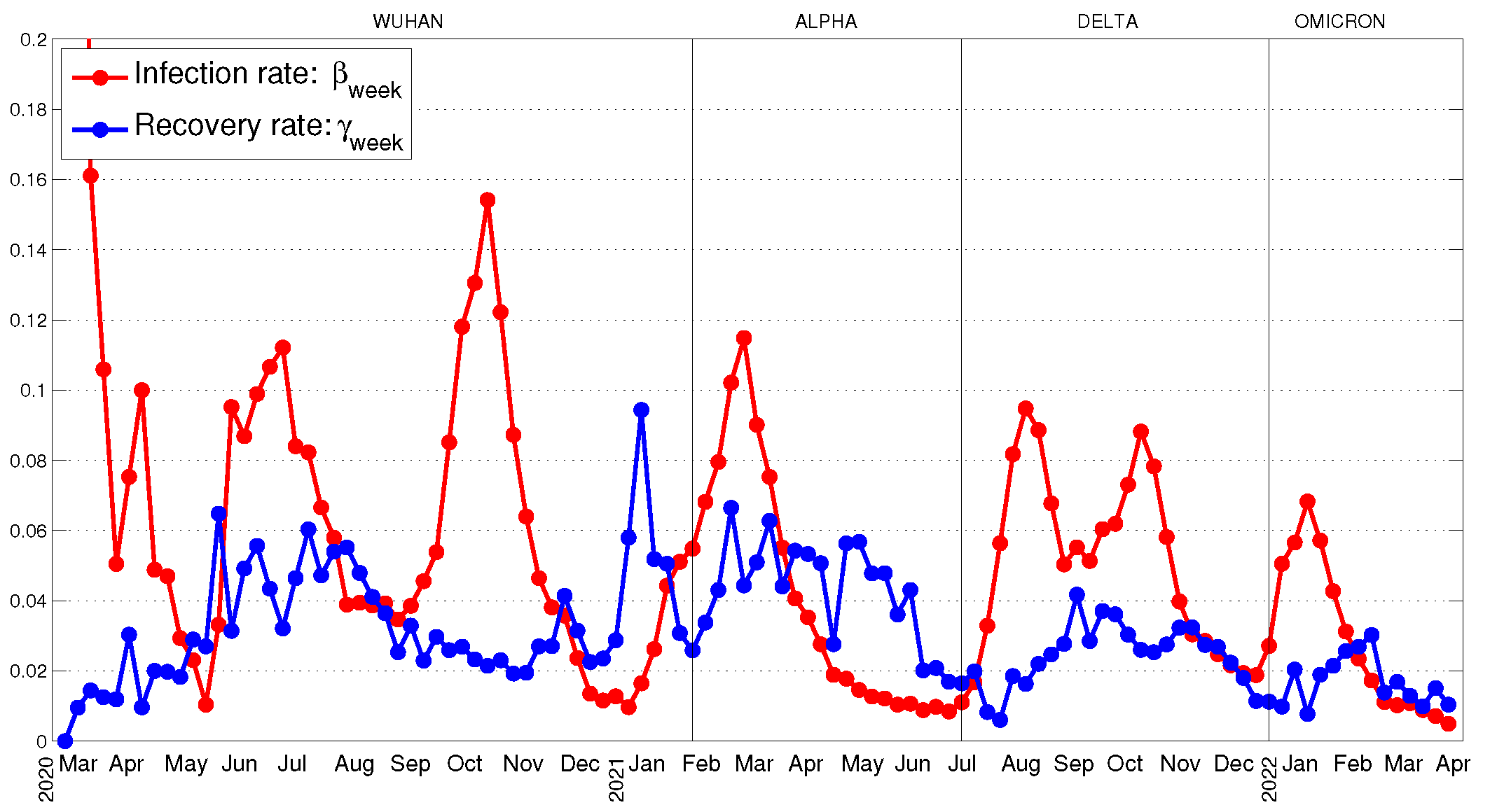
The Wuhan is usually used as a name of the first variant of the virus. To avoid possible misunderstanding, we note that, in the following Figure 2, Figure 3 and Figure 4, we point out the names of different variants (Wuhan, Alpha, Delta, Omicron) of SARS-CoV-2 and the corresponding periods in which they dominated in Bulgaria.
We observe that the infection rate decreases at the time of partial lockdowns (27 October 2020, 22 March 2021) or when strong rules and restrictions (21 October 2021) were imposed. The above-mentioned infection rate has been decreasing since green certificates were introduced (21 October 2021) as a preventive measure. On the other hand, the infection rate increased rapidly with the beginning of the first (the autumn of 2020) and second (the spring of 2021) waves and with the invasion of Delta (22 July 2021) or Omicron (2 January 2022) variants of SARS-CoV-2 in Bulgaria. We observe the following relations for the infection rate values for the first two weeks of Delta () or Omicron (o) waves and . The variation in infection rate for the Omicron variant is less than for the other virus variants. The reason for this is that the measures of social distancing were weak during the Omicron wave. This behavior of the Omicron infection rate causes a big wave which reaches its peak faster than the Delta wave. At the same time, the peaks of the recovery rate follow the peaks of the infection rate with some delay.
The obtained weekly average values of the vaccination parameter and mortality rate are given in Figure 3.
We observe that the vaccination parameter increases with the introduction of green certificates in Bulgaria, but it is still the lowest rate in the European Union and one of the lowest rates globally. At the same time, the COVID-19 mortality rate in Bulgaria is one of the highest levels in the world. It is natural that the peaks of the mortality rate follow the peaks of the infection rate with some delay.
6. Numerical Solution of the Differential Problem
Using Bulgarian COVID-19 data, in Section 5, we already found the daily values , of the parameters in the discrete problem (19). A natural question that arises is: How close are they to the daily values of the parameters in the differential problem (1)?
In order to answer this question, we solve numerically a recurrent sequence of initial problems for differential equation systems. Each of these problems corresponds to one of the days of the considered period of the pandemic. We do this using the selected values of parameters , , , , , and the calculated values for parameters , , , . More precisely, using the built-in function ode45 in Matlab (see [39]), which implements a version of Runge–Kutta 4th/5th-order method, for , we solve the Cauchy problem , :
where
The values of functions , and (solution of the problem ) at the end of the day are used as initial data in the next problem which describe the quantitative changes over the day The obtained piecewise linear curve is shown in Figure 4.
Since the numbers of active cases are known, we will compare them with the values , obtained by the procedure, described above. To do this, we use two different norms—the one and the sup-norm , i.e.,
These results show that the suggested method for identification of the parameters in the discrete problem leads to the parameters’ values which are very close to the values of the time-dependent coefficients in the differential problem. We can use other discretizations of the SEIRS-VB model, based for example on an explicit or implicit Euler method, but better results give the suggested semi-implicit discretized model (19).
7. Short-Term Forecasting
In this section, we present a methodology for short-term prediction of the numbers of active cases (A), new daily cases, COVID-19 deaths () and cumulative number or recovered individuals (). We assume that the parameters’ values are known. The experiments are based on the parameter identification method developed in Section 4 and the results obtained in Section 5. One possible way is to predict the unknown parameters’ values for the short- term forecast period using their values (calculated in Section 5) for several days before this period. It is worth mentioning that, in order to solve the problem (see Algorithm for solving IDP in Section 4), we have to calculate the values
first and then, via (31), we obtain For that purpose, we predict the values of in order to make the forecast for numbers of individuals in the compartments of SEIRS-VB model more accurate. To fix the notations, let the first day of the forecast period be denoted by . Then, the last day of this forecast period will be denoted .
We denote by
the predicted values of the parameters, using the proposed methodology, in order to distinguish them from the corresponding official ground-true data , reported by the Bulgarian officials.
The last known values are and the last calculated values are , which are obtained using the last known parameter’s value . We will predict the values , and for .
We perform two sets of numerical experiments, related to predicting a 14-day-time-frame in the future, based on the available official data for Bulgaria up to the first day of the time-frame. These time-frames are: 18–31 October 2021 and 7–20 February 2022, respectively. During the first time-frame, the Delta variant of the virus was dominant, while, during the second time-frame, the Omicron variant dominated.
For each time-frame, we make the prediction in three steps:
Prediction step 1. It is easy to discover cases/weekdays dependency in the official data. For example, the officially reported cases for Saturday and Sunday (reported on Sunday and Monday, respectively) are much fewer than the cases for Monday (reported on Tuesday). The same is true if we compare a holiday with a working day of the week. For this reason, we assume dependency of the parameters’ values on the weekdays. To verify this assumption, we examine the ratios between any two consecutive daily parameter values over different 7-day periods before the forecast period. For example, we study the behavior of the ratios
and , defined in a similar way for , respectively. Let us note that all these ratios are known for . After analyzing them, we forecast in an appropriate way the values , , , .
Prediction step 2. The first predicted day is and the values of parameters for the day are known. Then, our forecast of parameters’ values for the day is
and for the next six days are as follows:
for . Similarly, for the next 7 days, we define
for .
In such a way, we predict all parameters’ values which are needed for calculating the number of individuals in each of the considered compartments.
Prediction step 3. Since the values and , for the last day before the considered forecast period are known, we can predict the number of individuals in each of these compartments during the period . Using (25) and the predicted daily values of parameters, we calculate the values and of the recovered individuals and COVID-19 deaths, respectively. Furthermore, using again the predicted daily values of the parameters and (29), we calculate the values of active cases and the new daily cases . More precisely, for each day of the considered time-frame, using the morning values , , the parameter values and the predicted values , we calculate (using (29)) and (using (25)).
7.1. The First Time-Frame 18–31 October 2021
This time-frame is related to the peak of new daily cases of the wave caused by Delta variant of the virus. The reported cases on October 19th are considered as the values for October 18 th and so on. We consider the known ratios and for the last seven weeks before the first predicted day—18th October 2021, Monday. The values of the ratio are given in Table 3.
As we expected, almost always . Of course, there is an exception: because Monday, 6th September 2021 (Unification Day) is an official holiday in Bulgaria, and the reported new infected cases are much fewer than usual. An analogous situation is with and because 22nd September 2021 (The Independence Day in Bulgaria) is also a holiday. Such values should not be used in prediction of and .
On the other hand, the values in Table 3 show that, in each column, during almost all considered weeks. That is why we set in prediction step 1
for
Now, using (37)–(39) in prediction step 2, we derive the desired values . The behavior of the other ratios in the considered seven weeks is similar, and, in the same manner (as (40)), we predict other daily parameters’ values. Finally, we can make the prediction step 3.
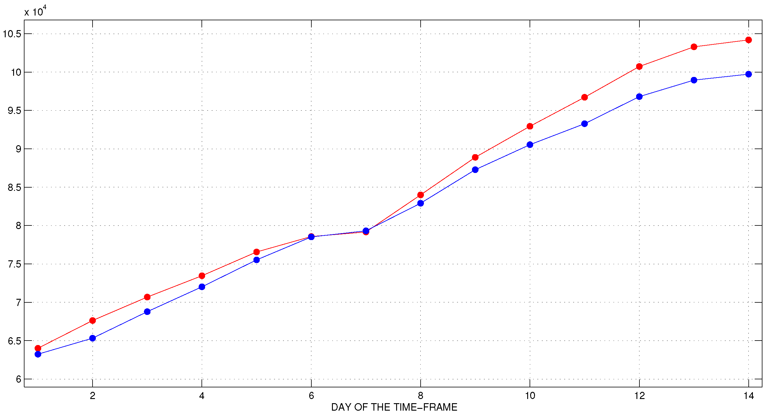
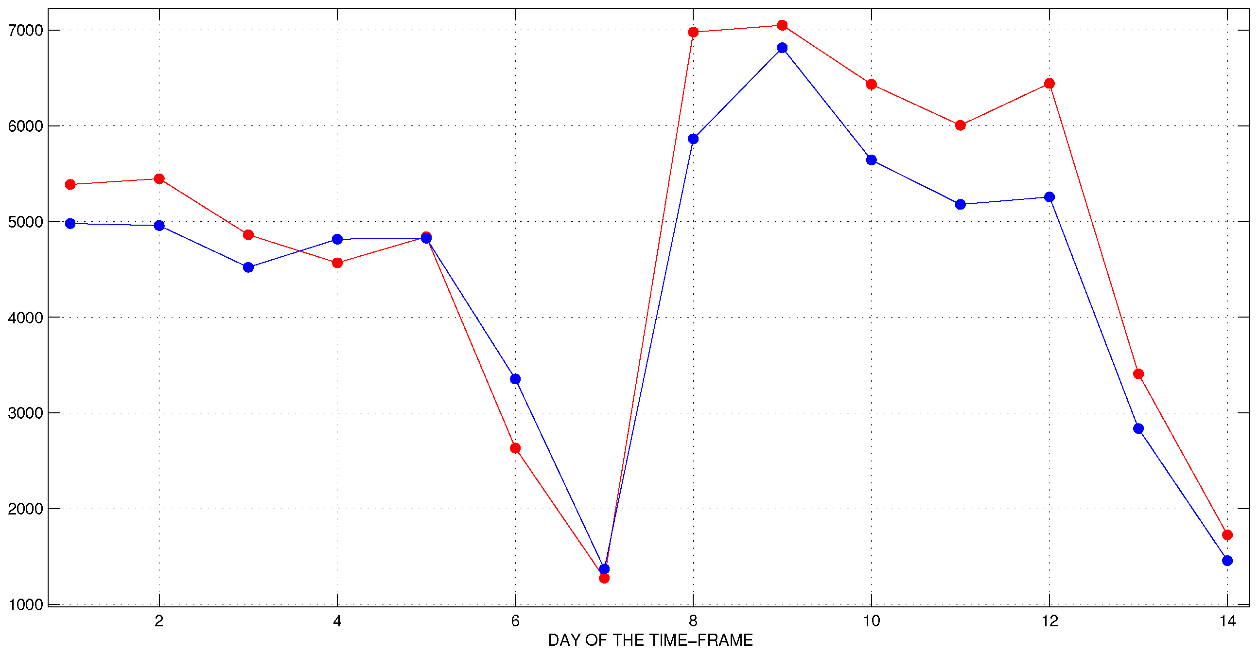
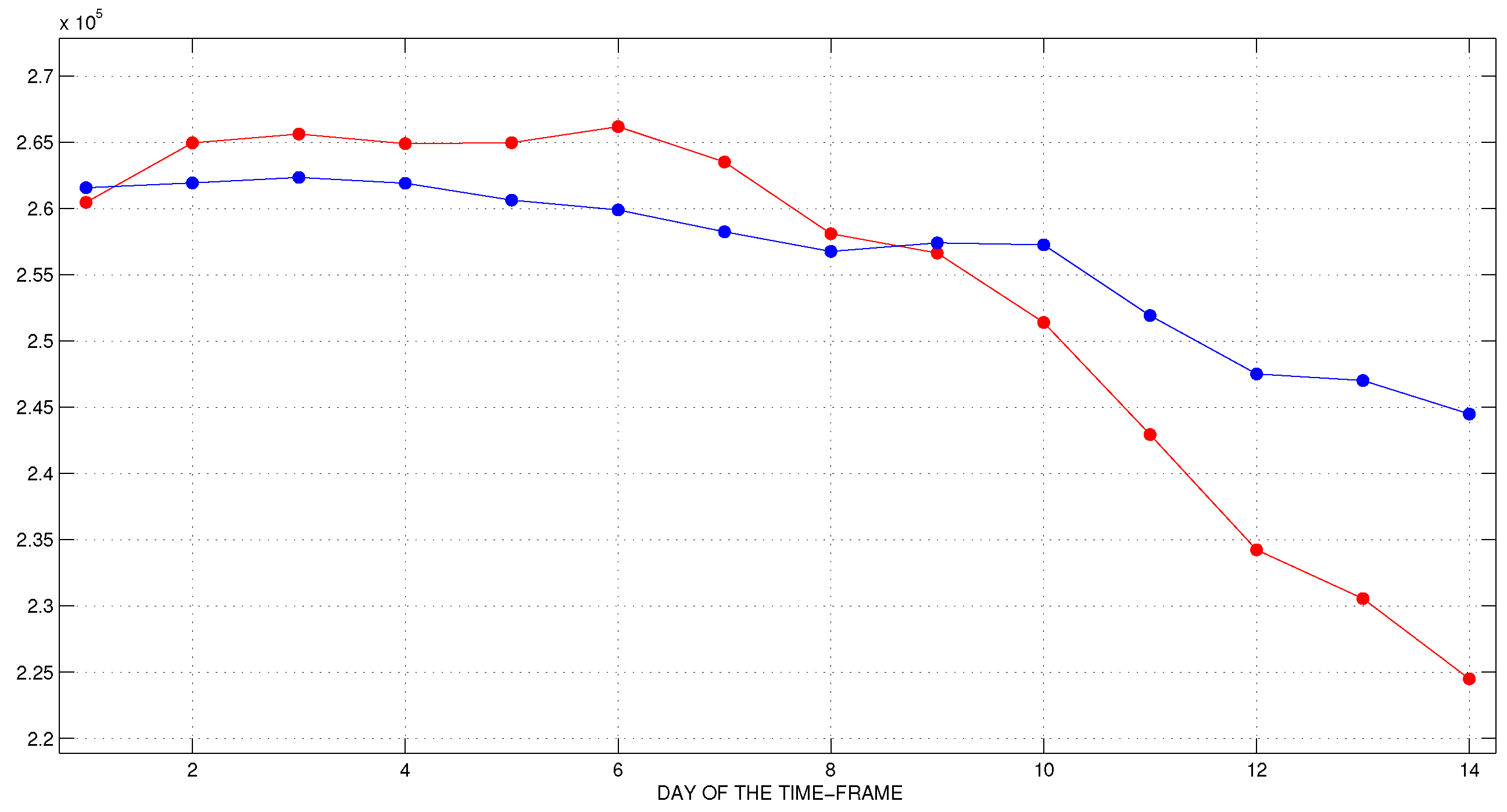
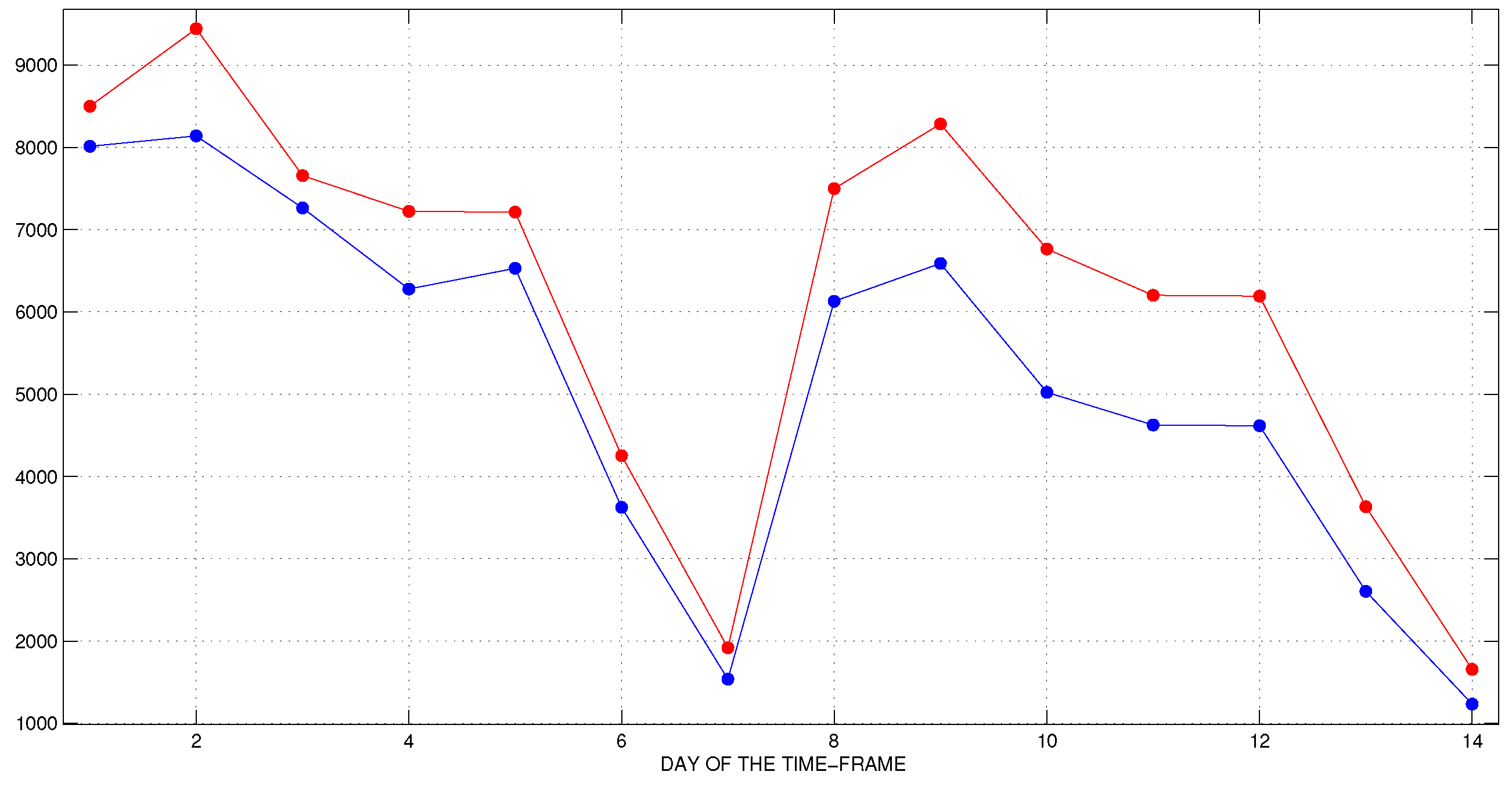
The experimental comparison between the official data and our prediction for the first time-frame is illustrated in Figure 5, Figure 6, Figure 7 and Figure 8. The official data are in the blue color and the predicted values are in the red color.
We observe a very good agreement between the predicted and the confirmed data during the first and the second week of the time-frame. However, the forecast for the first week is more accurate than for the second. It is interesting that, with this experiment, we predict the exact day of the peak of new daily cases and even the numbers of the predicted and reported cases on this day are very close. The number of recovered individuals and COVID-19 deaths are also fitted very well.
7.2. The Second Time-Frame 7–20 February 2022
This time-frame is related to the peak of active cases of the wave caused by the Omicron variant of the virus. Actually, in Bulgaria, this is the pandemic’s tallest peak (see Figure 4). Because of the very fast invasion of the Omicron variant, the peak has been reached only four weeks after the first confirmed cases with this variant. We consider again the known ratios and for the last seven weeks before the first predicted day—7th February 2022. Behavior of is similar to the Delta wave, wile oscillates (see Table 5).
Since the behavior of is very different from behavior of and in contrast to the first time-frame (see (40)) in prediction step 1, we set
In a similar way, we calculate and for
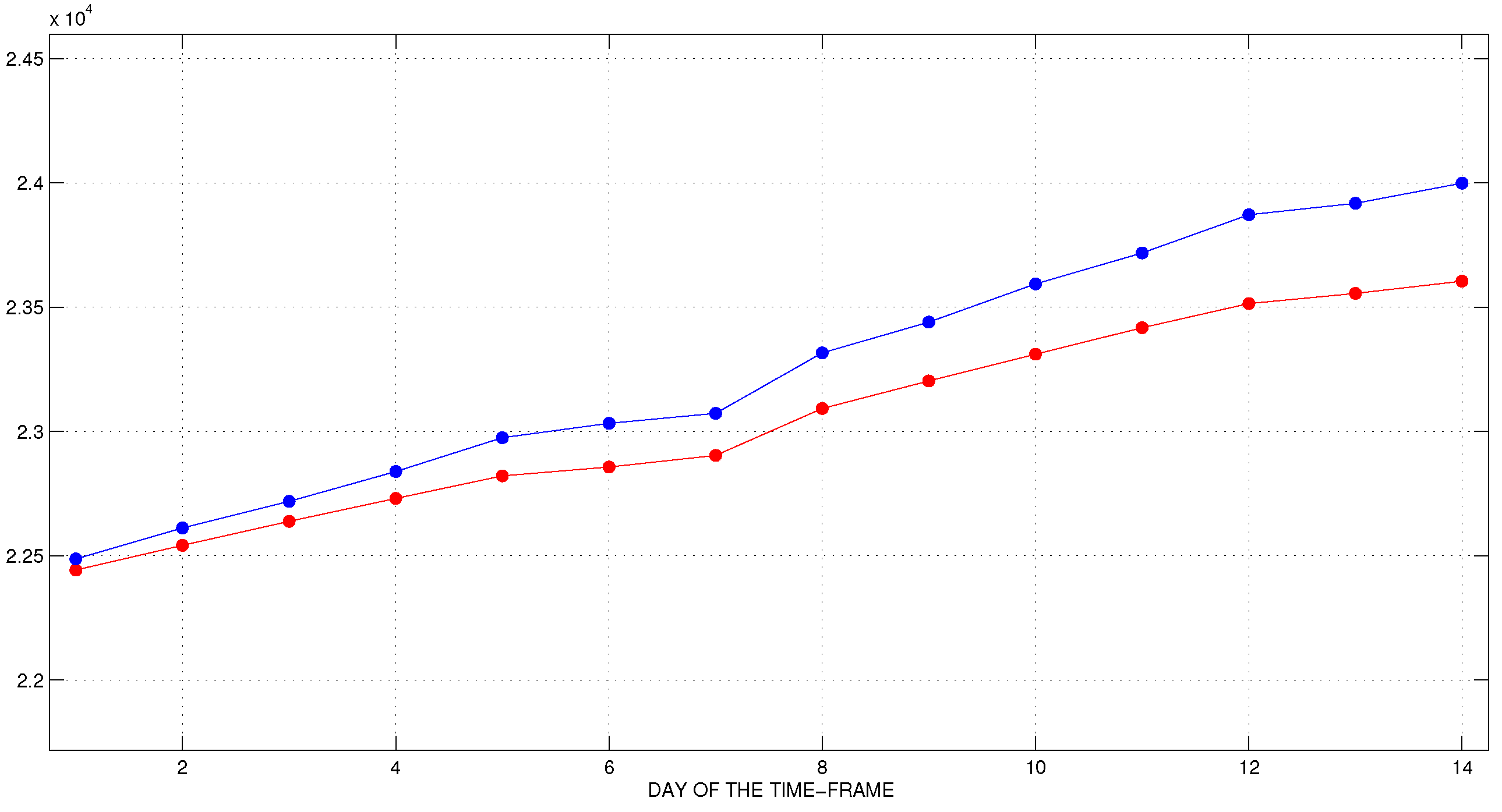
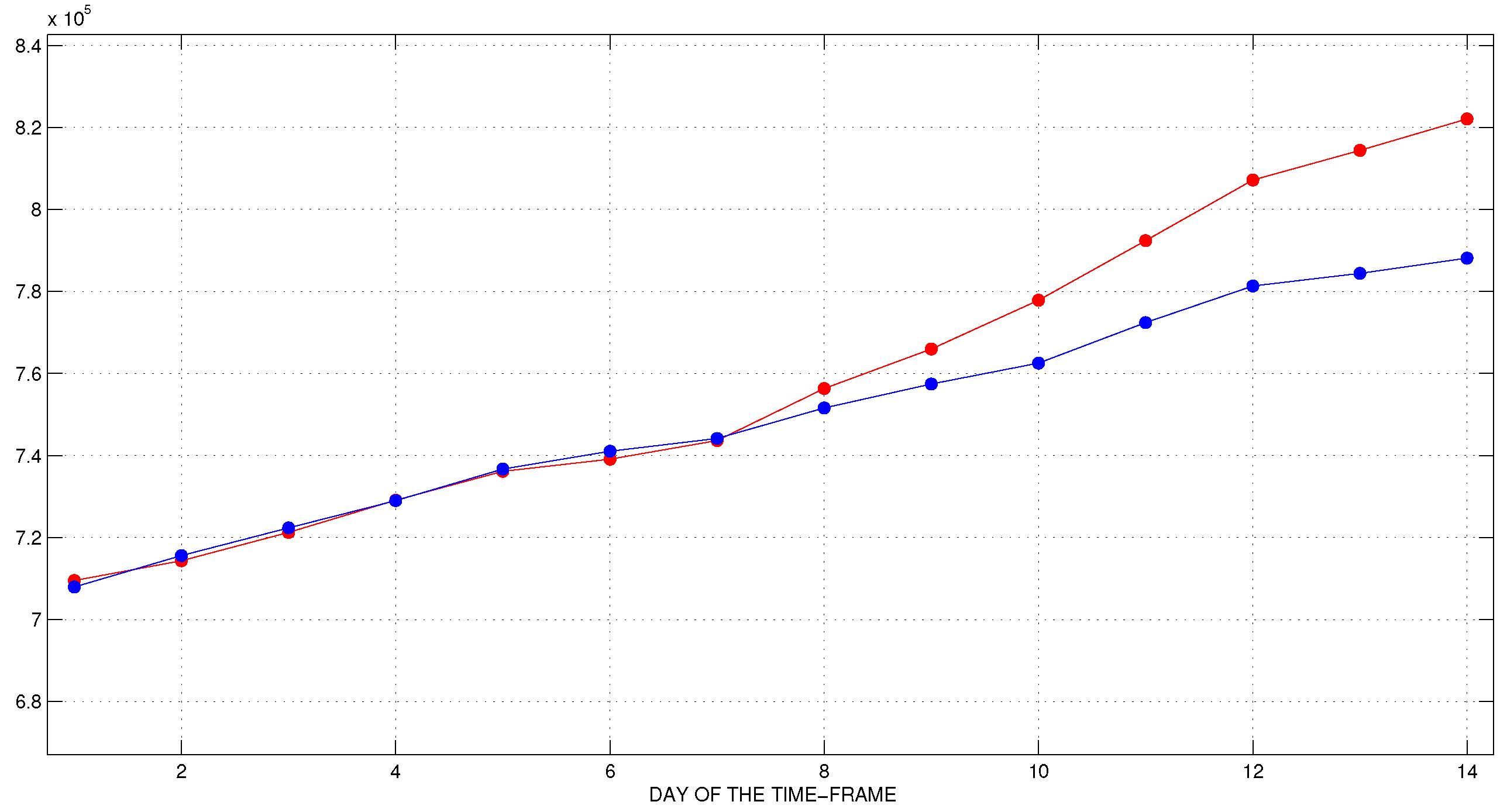
To predict the daily values of parameters (prediction step 2), we use the same methodology as in the prediction of the first time-frame. Now, we are able to make a prediction step 3. The comparison between the official data and our prediction for the second time-frame is illustrated in Figure 9, Figure 10, Figure 11 and Figure 12. The official data are in the blue color and the predicted data are in the red color.
We observe a good agreement between the predicted and the reported data. The peak of active cases and the number of COVID-19 deaths are fitted very well. The predicted active cases for the second week are smaller than the officially documented ones and the daily differences between the two plots are larger than in the first time-frame. At the same time, the predicted number of new cases is larger than the reported ones. The number of recovered individuals is fitted well. This experiment shows that the proposed methodology works well even in such a delicate situation, when the parameters change their behavior quite significantly.
The relative weekly-based errors for the compartments for both the first and the second 14-days-time-frames are documented in Table 6.
We observe a good agreement between the corresponding error margins of the two norms and (see (34) and (35), Table 4 and Table 6), which suggest robustness of the proposed model with respect to the norm choice within the family. Let us note that, for the active cases, deaths and recovered individuals, we predict the cumulative number, while, for the dally cases, we consider only the new infectious individuals on the corresponding day. Thus, the relative forecast errors are naturally larger for the new daily cases than the corresponding forecast errors for the other compartments.
8. Discussion
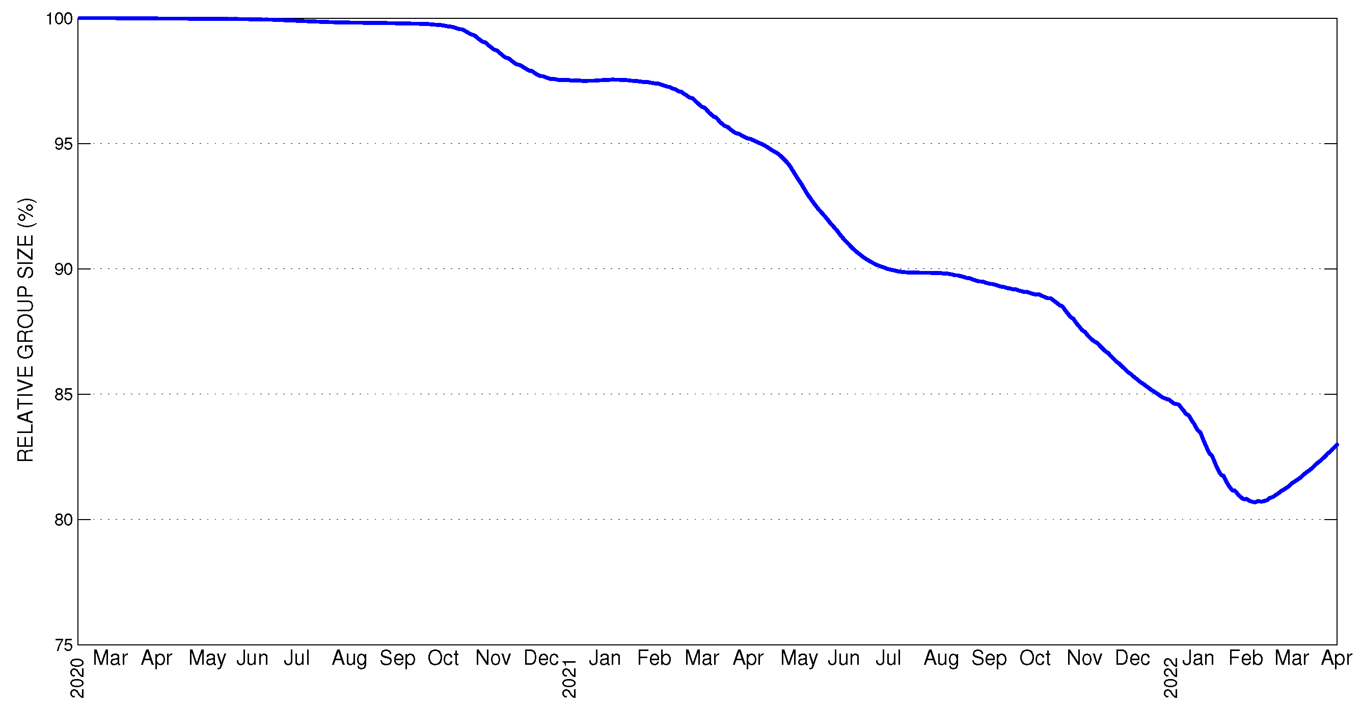
Actually, since the considered model takes into account some factors that play an essential role in the viral diseases’ dynamics such as re-susceptibility, duration of the latency period (specific for each of the dominant virus variants) and the vaccines’ effectiveness. After finding the models parameters in Section 5, we are able to calculate the daily number of Susceptible individuals , Recovered individuals , Vaccinated susceptible individuals and individuals with antibodies . It should be noted that there is no official data on the size of these compartments, as public data sets contain information on the cumulative number of recovered and vaccinated persons. That is why the results obtained by our model can be very useful. For example, in Figure 13, we give the daily relative size of the compartment of all susceptible individuals in Bulgaria, which is closely related to the determination of the herd immunity threshold (see [40]).
In the months following the emergence of SARS-CoV-2, “herd immunity” was frequently cited as the long-term destination of the COVID-19 pandemic. However, since the “Delta” variant appeared (end of August 2021), our idea was to calculate in our mathematical-computer model the level of “herd immunity”, and it seemed to be more than 90%, which is impossible to be achieved. From our group, we announced this fact and discussed it at a Conference of UBM on 5 September 2021. At the same time, at least two publications [41,42] in this area appeared in the USA with discussions on how it is better to react to this situation?
The idea of herd immunity primarily supports high vaccination coverage and the acquisition of natural immunity due to illness.
Although COVID-19 vaccines provide some protection against infection and a mild form of COVID-19, they have failed to stop the transmission of the virus, especially for the highly transmitted delta and omicron variants. An excellent example in this regard was the decision of the United Kingdom Government to allow the opening of society based on a high percentage of vaccination coverage, which minimizes the risk of severe COVID-19 and death. Indeed, significantly increased mortality was not achieved, but the daily incidence reached over 270,000 new cases per day with Omicron. This decision has demonstrated that the purpose of herd immunity, even in a resource-rich environment, is unattainable [43].
An interesting study based on 17 cases of genetically confirmed re-infection with COVID-19 showed that one immunocompromised patient had mild symptoms in the first infection but developed severe symptoms leading to death in the second infection. Overall, 68.8% (11/16) had a similar burden; 18.8% (3/16) had worse symptoms, and 12.5% (2/16) had milder symptoms with the second episode. The conclusion is that, in general, re-infection with different strains is possible and, in some cases, may develop more severe infections with the second episode [44].
Recently, John Ashton, in his review, claimed that the dominance of politics over science as manifested by the rush to abandon all measures of virus control has led to the emergence of a dominant domestic narrative that the pandemic is over. The assumption has been spreading that COVID-19 will only be of nuisance value on a par with the flu in the future. Such a decision has already been taken in Spain. In addition, this theory plays down the associated morbidity and mortality associated with COVID-19 compared to influenza [45].
A similar reaction came from EMA’s vaccine strategy chief Marco Cavaleri almost simultaneously. They also discussed what would be better to do in such a situation. The question is: How should we be thinking about “herd immunity” to COVID-19? According to today’s data for the rate of “herd immunity”, we can not eliminate SARS-CoV-2, and the virus continues to circulate. We do not have enough effective vaccines, and due to the high mutation rate of the virus, the vast majority of the population still can be exposed. That is why we should keep working, predicting and monitoring the situation according to this reality!
Once again, we note that all results in this study were obtained using official data sets. A debatable question is what is the true number of infections with SARS-CoV-2. We cannot answer this question, but we suppose that the most accurate among the reported data are the numbers of COVID-19 deaths. Here we will discuss the results of our study on mortality from COVID-19 and additional mortality during the ongoing pandemic in Bulgaria. Using the available data for deaths in Bulgaria (see [35]) for the last five years 2015, 2016, 2017, 2018 and 2019 before the beginning of the COVID-19 pandemic, we calculate the expected and excess deaths per 100,000 population for the considered period of the pandemic.
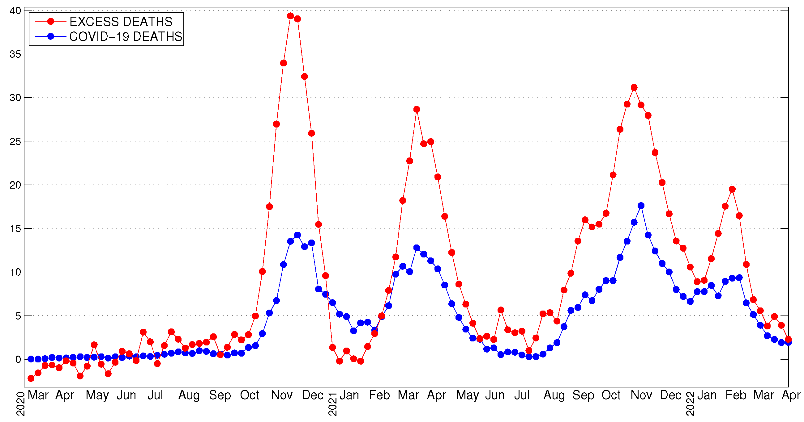
An interesting observation is that the times of the excess deaths peaks and the peaks of COVID-19 deaths in Bulgaria coincide (see Figure 14). We will note that the excess deaths during the peak periods are more than twice as big as COVID-19 deaths. This could mean that the COVID-19 is about twice as deadly or that their measures taken to limit its spread cause death as much as the virus itself. In the same time, the WHO reported (see [46]) that the deaths associated with the COVID-19 pandemic between 1 January 2020 and 31 December 2021 were approximately 14.9 million. Hence, globally, the excess deaths from COVID-19 pandemic is about three times more than the reported. Further study is warranted to investigate how the different restriction measures and the vaccination strategy used affect the transmission rate and COVID-19 mortality rate in Bulgaria or in other countries with high mortality.
9. Conclusions
In the present paper, we formulate a new time-dependent deterministic model SIRS-VB with vaccination and vital dynamics. Since available measurements were made at the end of each day of the pandemic, we introduce a semi-implicit finite difference scheme with a step size of 1 day, and then we provide an algorithm for identification of the parameters in the obtained discrete problem. Furthermore, we conduct numerical experiments which show that the calculated parameters values are very close to the values of parameters in the original differential problem. This allows us to calculate realistic values for all compartments in the considered deterministic model by using the suggested identification procedure. The presented study cannot predict the emergence of a new variant or strain of the virus or a new wave caused by it. However, the results in Section 7 show that, when a new wave appears, the model can be efficiently used for making 14-day forecasts for daily numbers of the new infectious cases and the new deaths. The presented prediction methodology is based on the cases/weekdays dependence of the real-time existing data. It requires a very careful analysis of the available data, taking into account the atypical daily values of the parameters during recent weeks and whether such type of values are expected during the forecast period.
Author Contributions
Investigation, S.M., N.P. and T.H.; Methodology, S.M., N.P., I.U. and T.H.; Writing—original draft, N.P. and T.H.; Writing—review & editing, S.M. All authors have read and agreed to the published version of the manuscript.
Funding
The work of Nedyu Popivanov and Tsvetan Hristov was partially supported by Bulgarian NSF under Grant KP-06-H52/4, 2021 and by Sofia University under Grant 80-10-26/2022. The work of Iva Ugrinova was partially supported by the Bulgarian Ministry of Education under Grant D 01-397/18 December 2020.
Institutional Review Board Statement
Not applicable.
Informed Consent Statement
Not applicable.
Data Availability Statement
The Codes used for this study are available upon request from the corresponding author.
Conflicts of Interest
The authors declare no conflict of interest.
References
- Margenov, S.; Popivanov, N.; Ugrinova, I.; Harizanov, S.; Hristov, T. Parameters Identification and Forecasting of COVID-19 Transmission Dynamics in Bulgaria with Mass Vaccination Strategy. AIP Conf. Proc. 2022, in press.
- Bjørnstad, O.N.; Shea, K.; Krzywinski, M.; Altman, N. The SEIRS Model for Infectious Disease Dynamics. Nat. Methods 2020, 17, 557–558. [Google Scholar] [CrossRef]
- Mehra, A.; Shafieirad, M.; Abbasi, Z.; Zamani, I. Parameter Estimation and Prediction of COVID-19 Epidemic Turning Point and Ending Time of a Case Study on SIR/SQAIR Epidemic Models. Comput. Math. Methods Med. 2020, 2020, 1465923. [Google Scholar] [CrossRef]
- Paul, S.; Lorin, E. A Hybrid Approach to Predict COVID-19 Cases Using Neural Networks and Inverse Problem. Available online: https://www.researchgate.net/publication/360069791 (accessed on 1 May 2022).
- Al-Hadeethi, Y.; Ramley, I.F.; Sayyed, M.I. Convolution Model for COVID-19 Rate Predictions and Health Effort Levels Computation for Saudi Arabia, France, and Canada. Sci. Rep. 2021, 11, 22664. [Google Scholar] [CrossRef]
- Krivorotko, O.; Kabanikhin, S.; Sosnovskaya, M.; Andornaya, D. Sensitivity and Identifiability Analysis of COVID-19 Pandemic Models. Vavilov J. Genet. Breed. 2021, 25, 82–91. [Google Scholar] [CrossRef] [PubMed]
- Krivorotko, O.; Kabanikhin, S.; Zyatkov, N.; Prikhodko, A.; Prokhoshin, N.; Shishlenin, M. Mathematical Modeling and Forecasting of COVID-19 in Moscow and Novosibirsk Region. Numer. Anal. Appl. 2020, 13, 332–348. [Google Scholar] [CrossRef]
- Kabanikhin, S.I.; Bektemesov, M.A.; Bektemessov, J.M. Mathematical Model for Medium Term Covid 19 Forecasts in Kazakhstan. J. Math. Mech. Comput. Sci. Appl. Math. 2021, 111, 95–106. [Google Scholar] [CrossRef]
- Ko, G.S.; Yoon, T. Short-Term Prediction Methodology of COVID-19 Infection in South Korea. COVID 2021, 1, 35. [Google Scholar] [CrossRef]
- Zhao, H.; Merchant, N.N.; McNulty, A.; Radcliff, T.A.; Cote, M.J.; Fischer, R.S.B.; Sang, H.; Ory, M.G. COVID-19: Short Term Prediction Model Using Daily Incidence Data. PLoS ONE 2021, 16, e0250110. [Google Scholar] [CrossRef]
- Kovacevic, R.; Stilianakis, N.; Veliov, V. A Distributed Optimal Control Model Applied to COVID-19 Pandemic. SIAM J. Control. Optim. 2022, 60, 221–245. [Google Scholar] [CrossRef]
- Yang, Q.; Yi, C.; Vajdi, A.; Cohnstaedt, L.W.; Wu, H.; Guo, X.; Scoglio, C.M. Short-term Forecasts and Long-term Mitigation Evaluations for the COVID-19 Epidemic in Hubei Province, China. Infect. Model. 2020, 5, 563–574. [Google Scholar] [CrossRef] [PubMed]
- Ghostine, R.; Gharamti, M.; Hassrouny, S.; Hoteit, I. An Extended SEIR Model with Vaccination for Forecasting the COVID-19 Pandemic in Saudi Arabia Using an Ensemble Kalman Filter. Mathematics 2021, 9, 636. [Google Scholar] [CrossRef]
- Engbert, R.; Rabe, M.; Kliegl, R.; Reich, S. Sequential Data Assimilation of the Stochastic SEIR Epidemic Model for Regional COVID-19 Dynamics. Bull. Math. Biol. 2021, 83, 1–16. [Google Scholar] [CrossRef]
- Margenov, S.; Popivanov, N.; Ugrinova, I.; Harizanov, S.; Hristov, T. Mathematical and Computer Modeling of COVID-19 Transmission Dynamics in Bulgaria by Time-depended Inverse SEIR Model. AIP Conf. Proc. 2021, 2333, 090024. [Google Scholar] [CrossRef]
- Marinov, T.; Marinova, R. Dynamics of COVID-19 using inverse problem for coefficient identification in SIR epidemic models. Chaos Solitons Fractals X 2020, 5, 100041. [Google Scholar] [CrossRef]
- Gurova, S.-M. COVID-19: Study of the spread of the pandemic in Bulgaria. In Proceedings of the 22nd European Young Statisticians Meeting, Athens, Greece, 6–10 December 2021; Volume 136, pp. 40–44. [Google Scholar]
- Kounchev, O.; Simeonov, G.; Kuncheva, Z. Estimation of the Duration of Covid-19 Epidemic in a Single Country, with or without Vaccinations. The Case of Bulgaria and Germany. C. R. L’Academie Bulg. Des Sci. 2021, 74, 677–686. [Google Scholar]
- Ma, W.; Zhao, Y.; Guo, L.; Chen, Y. Qualitative and quantitative analysis of the COVID-19 pandemic by a two-side fractional-order compartmental model. ISA Trans. 2022, 124, 144–156. [Google Scholar] [CrossRef]
- Ma, N.; Ma, W.; Li, Z. Multi-Model Selection and Analysis for COVID-19. Fractal Fract. 2021, 5, 120. [Google Scholar] [CrossRef]
- Olivares, A.; Staffetti, E. Uncertainty Quantification of a Mathematical Model of COVID-19 Transmission Dynamics with Mass Vaccination Strategy. Chaos Solitons Fractals 2021, 146, 110895. [Google Scholar] [CrossRef]
- Angelov, G.; Kovacevic, R.; Stilianakis, N.; Veliov, V. Optimal Vaccination Strategies Using a Distributed Epidemiological Model Applied to COVID-19; Research Report; SWM Vienna University of Technology: Vienna, Austria, 2021; pp. 1–22. Available online: https://orcos.tuwien.ac.at/fileadmin/t/orcos/Research_Reports/2021-02.pdf (accessed on 1 May 2022).
- Iboid, E.; Ngonghalab, C.; Gumel, A. Will an imperfect vaccine curtail the COVID-19 pandemic in the U.S.? Infect. Dis. Model. 2020, 5, 510–524. [Google Scholar] [CrossRef]
- Safarishahrbijari, A.; Lawrence, T.; Lomotey, R.; Liu, J.; Waldner, C.; Osgood, N. Particle Filtering in a SEIRV Simulation Model of H1N1 Influenza. In Proceedings of the 2015 Winter Simulation Conference, Huntington Beach, CA, USA, 6–9 December 2015; pp. 1240–1251. [Google Scholar] [CrossRef]
- Carcione, J.; Santos, J.; Bagaini, C.; Ba, J. A Simulation of a COVID-19 Epidemic Based on a Deterministic SEIR Model. Front. Public Health 2020, 8, 230. [Google Scholar] [CrossRef] [PubMed]
- Singh, R.A.; Lal, R.; Kotti, R.R. Time-discrete SIR model for COVID-19 in Fiji. Epidemiol. Infect. 2022, 150, e75. [Google Scholar] [CrossRef] [PubMed]
- Kermack, W.; McKendrick, A. A Contribution to the Mathematical Theory of Pandemics. Proc. R. Soc. Lond. Ser. A 1927, 115, 700–721. [Google Scholar]
- Liu, M.; Cao, J.; Liang, J.; Chen, M. Epidemic-logistics Modeling: A New Perspective on Operations Research, 1st ed.; Springer: Singapore, 2020; p. 287. [Google Scholar] [CrossRef]
- Sun, C.; Hsieh, Y.-H. Global Analysis of an SEIR Model with Varying Population Size and Vaccination. Appl. Math. 2010, 34, 2685–2697. [Google Scholar] [CrossRef]
- Trawicki, M.B. Deterministic Seirs Epidemic Model for Modeling Vital Dynamics, Vaccinations, and Temporary Immunity. Mathematics 2017, 5, 7. [Google Scholar] [CrossRef]
- Hartman, P. Ordinary Differential Equations, 2nd ed.; Society for Industrial and Applied Mathematics: Philadelphia, PA, USA, 2002; p. 624. [Google Scholar]
- Menni, C.; Valdes, A.M.; Polidori, L.; Antonelli, M.; Penamakuri, S.; Nogal, A.; Louca, P.; May, A.; Figueiredo, J.C.; Hu, C.; et al. Symptom prevalence, duration, and risk of hospital admission in individuals infected with SARS-CoV-2 during periods of omicron and delta variant dominance: A prospective observational study from the ZOE COVID Study. Lancet 2022, 399, 1618–1624. [Google Scholar] [CrossRef]
- The Open Data Portal of the Republic of Bulgaria. Available online: https://data.egov.bg (accessed on 12 April 2022).
- The Official Bulgarian Unified Information Portal. Available online: https://coronavirus.bg/ (accessed on 12 April 2022).
- Information System INFOSTAT of the National Statistical Institute of the Republic of Bulgaria. Available online: https://infostat.nsi.bg/ (accessed on 24 April 2022).
- European Centre for Disease Prevention and Control (ECDC). Available online: https://www.ecdc.europa.eu (accessed on 24 April 2022).
- WHO Coronavirus (COVID-19) Dashboard. Available online: https://covid19.who.int/ (accessed on 12 April 2022).
- European Medicines Agency. Vaccines Authorised in the European Union (EU) to Prevent COVID19. Available online: https://www.ema.europa.eu/en/human-regulatory/overview/public-health-threats/coronavirus-disease-covid-19/treatments-vaccines/vaccines-covid-19/covid-19-vaccines-authorised (accessed on 24 April 2022).
- MathWorks. Matlab Documentation. Available online: https://www.mathworks.com/help/matlab/ref/ode45.html (accessed on 24 April 2022).
- Hethcote, H. The Mathematics of Infectious Diseases. SIAM Rev. 2000, 42, 599–653. [Google Scholar] [CrossRef] [Green Version]
- D’Souza, G.; Dowdy, D. Rethinking Herd Immunity and the Covid-19 Response End Game, Johns Hopkins Bloomberg School of Public Health. 2021. Available online: https://publichealth.jhu.edu/2021/what-is-herd-immunity-and-how-can-we-achieve-it-with-covid-19 (accessed on 1 May 2022).
- Barker, P.; Hartley, D.; Beck, A.F.; Oliver, G.; Sampath, B.; Roderick, T.; Miff, S. Rethinking Herd Immunity: Managing the Covid-19 Pandemic in a Dynamic Biological and Behavioral Environment. NEJM Catal. Innov. Care Deliv. 2021, 1–9. Available online: https://catalyst.nejm.org/doi/pdf/10.1056/CAT.21.0288 (accessed on 1 May 2022).
- Madhi, S. COVID-19 herd immunity v. learning to live with the virus. S. Afr. Med. J. 2021, 111, 852–856. [Google Scholar] [CrossRef]
- Wang, J.; Kaperak, C.; Sato, T.; Sakuraba, A. COVID-19 reinfection: A rapid systematic review of case reports and case series. J. Investig. Med. 2021, 69, 1253–1255. [Google Scholar] [CrossRef]
- Ashton, J. COVID-19 and herd immunity. J. R. Soc. Med. 2022, 115, 76–77. [Google Scholar] [CrossRef] [PubMed]
- WHO, 14.9 Million Excess Deaths Associated with the COVID-19 Pandemic in 2020 and 2021. Available online: https://www.who.int/news/item/05-05-2022-14.9-million-excess-deaths-were-associated-with-the-covid-19-pandemic-in-2020-and-2021 (accessed on 8 May 2022).
Figure 2.
The weekly average values of infection and recovery rates.

Figure 3.
The weekly average values of vaccination parameter and mortality rate .

Figure 4.
Confirmed data and SEIRS-VB model’s curve of active cases.

Figure 5.
The first time-frame. Official (blue) and predicted (red) data for active cases.

Figure 6.
The first time-frame. Official (blue) and predicted (red) data for the new daily cases.

Figure 7.
The first time-frame. Official (blue) and predicted (red) data for cumulative number of COVID-19 deaths.
Figure 7.
The first time-frame. Official (blue) and predicted (red) data for cumulative number of COVID-19 deaths.

Figure 8.
The first time-frame. Official (blue) and predicted (red) data for cumulative number of recovered individuals.
Figure 8.
The first time-frame. Official (blue) and predicted (red) data for cumulative number of recovered individuals.

Figure 9.
The second time-frame. Official (blue) and predicted (red) data for active cases.

Figure 10.
The second time-frame. Official (blue) and predicted (red) data for the new daily cases.

Figure 11.
The second time-frame. Official (blue) and predicted (red) data for the cumulative number of COVID-19 deaths.
Figure 11.
The second time-frame. Official (blue) and predicted (red) data for the cumulative number of COVID-19 deaths.

Figure 12.
The second time-frame. Official (blue) and predicted (red) data for cumulative number of recovered individuals.
Figure 12.
The second time-frame. Official (blue) and predicted (red) data for cumulative number of recovered individuals.

Figure 13.
The relative size of the susceptible individuals calculated with the SEIRS-VB model.

Figure 14.
Excess and COVID-19 deaths (per 100,000 population) on a weekly basis.


Table 1.
Parameters of the SEIRS-VB model.
| Parameter | Description | Units |
|---|---|---|
| birth rate | ||
| vaccination rate | ||
| vaccine effectiveness | ||
| vaccination parameter | ||
| transmission rate | 1/days | |
| recovery rate | 1/ days | |
| latency rate | 1/days | |
| natural mortality rate | ||
| mortality rate of infectious people | ||
| reinfection rate of recovered individuals | 1/days | |
| reinfection rate of vaccinated individuals | 1/days | |
| antibody rate | 1/days |
Table 2.
The given parameter’s values.
| Parameter | Description | Values |
|---|---|---|
| birth rate | ||
| natural mortality rate | ||
| latency period | 7 days 1, 6 days 2, 5 days 3, 4 days 4 | |
| time taken for antibodies to develop | 14 days | |
| duration of vaccine-based immunity | 180 days | |
| duration of disease-based immunity | 180 days | |
| vaccine effectiveness |
for 1 Wuhan variant, 2 Alpha variant, 3 Delta variant, 4 Omicron variant.
Table 3.
Documentation of the ratio .
| Mon/Sun | Tue/Mon | Wed/Tue | Thur/Wed | Fri/Thur | Sat/Fri | Sun/Sat | |
|---|---|---|---|---|---|---|---|
| k | |||||||
| 5.573 | 0.999 | 0.959 | 0.957 | 1.081 | 0.543 | 0.536 | |
| 5.452 | 1.021 | 0.887 | 0.905 | 1.079 | 0.502 | 0.499 | |
| 5.098 | 1.014 | 0.832 | 0.957 | 1.020 | 0.587 | 0.418 | |
| 5.138 | 0.929 | 0.388 | 2.156 | 1.037 | 0.545 | 0.478 | |
| 4.559 | 1.015 | 0.918 | 0.926 | 1.097 | 0.503 | 0.482 | |
| 1.386 | 2.957 | 0.975 | 0.833 | 0.998 | 0.559 | 0.481 | |
| 4.624 | 0.982 | 0.850 | 0.896 | 1.048 | 0.521 | 0.572 |
Table 4.
Relative errors of the prediction for week 1 (18–24 October 2021) and week 2 (25–31 October 2021).
Table 4.
Relative errors of the prediction for week 1 (18–24 October 2021) and week 2 (25–31 October 2021).
| Compartment | Error (, Week) | Error (, Week) | Error (, Week) | Error (, Week) |
|---|---|---|---|---|
| Active cases | 0.018 | 0.034 | 0.029 | 0.042 |
| New daily cases | 0.090 | 0.138 | 0.132 | 0.168 |
| Deaths | 0.005 | 0.013 | 0.007 | 0.016 |
| Recovered | 0.001 | 0.001 | 0.002 | 0.002 |
Table 5.
Documentation of the ratio .
| Mon/Sun | Tue/Mon | Wed/Tue | Thur/Wed | Fri/Thur | Sat/Fri | Sun/Sat | |
|---|---|---|---|---|---|---|---|
| k | |||||||
| 2.311 | 0.857 | 1.051 | 1.306 | 1.135 | 0.557 | 0.593 | |
| 4.249 | 0.459 | 1.790 | 0.971 | 0.656 | 0.292 | 2.444 | |
| 0.447 | 3.186 | 0.490 | 0.442 | 5.049 | 0.649 | 1.101 | |
| 10.917 | 1.425 | 4.729 | 0.650 | 0.562 | 0.408 | 1.326 | |
| 1.229 | 2.100 | 0.565 | 2.221 | 0.401 | 2.655 | 0.047 | |
| 4.265 | 1.381 | 1.485 | 0.485 | 0.512 | 0.201 | 4.522 | |
| 8.402 | 0.878 | 0.734 | 0.950 | 0.237 | 0.681 | 1.293 |
Table 6.
Relative errors of the prediction for week 1 (7–13 February 2022) and week 2 (14–20 February 2022).
Table 6.
Relative errors of the prediction for week 1 (7–13 February 2022) and week 2 (14–20 February 2022).
| Compartment | Error (, Week) | Error (, Week) | Error (, Week) | Error (, Week) |
|---|---|---|---|---|
| Active cases | 0.015 | 0.048 | 0.023 | 0.077 |
| New daily cases | 0.107 | 0.230 | 0.137 | 0.210 |
| Deaths | 0.001 | 0.005 | 0.001 | 0.007 |
| Recovered | 0.001 | 0.028 | 0.002 | 0.041 |
Publisher’s Note: MDPI stays neutral with regard to jurisdictional claims in published maps and institutional affiliations. |
© 2022 by the authors. Licensee MDPI, Basel, Switzerland. This article is an open access article distributed under the terms and conditions of the Creative Commons Attribution (CC BY) license (https://creativecommons.org/licenses/by/4.0/).
Share and Cite
MDPI and ACS Style
Margenov, S.; Popivanov, N.; Ugrinova, I.; Hristov, T. Mathematical Modeling and Short-Term Forecasting of the COVID-19 Epidemic in Bulgaria: SEIRS Model with Vaccination. Mathematics 2022, 10, 2570. https://doi.org/10.3390/math10152570
AMA Style
Margenov S, Popivanov N, Ugrinova I, Hristov T. Mathematical Modeling and Short-Term Forecasting of the COVID-19 Epidemic in Bulgaria: SEIRS Model with Vaccination. Mathematics. 2022; 10(15):2570. https://doi.org/10.3390/math10152570
Chicago/Turabian StyleMargenov, Svetozar, Nedyu Popivanov, Iva Ugrinova, and Tsvetan Hristov. 2022. "Mathematical Modeling and Short-Term Forecasting of the COVID-19 Epidemic in Bulgaria: SEIRS Model with Vaccination" Mathematics 10, no. 15: 2570. https://doi.org/10.3390/math10152570
Note that from the first issue of 2016, this journal uses article numbers instead of page numbers. See further details here.