Artificial Neural Networking (ANN) Model for Drag Coefficient Optimization for Various Obstacles

Abstract

For various obstacles in the path of a flowing liquid stream, an artificial neural networking (ANN) model is constructed to study the hydrodynamic force depending on the object. The multilayer perceptron (MLP), back propagation (BP), and feed-forward (FF) network models were employed to create the ANN model, which has a high prediction accuracy and a strong structure. To be more specific, circular-, octagon-, hexagon-, square-, and triangular-shaped cylinders are installed in a rectangular channel. The fluid is flowing from the left wall of the channel by following two velocity profiles explicitly linear velocity and parabolic velocity. The no-slip condition is maintained on the channel upper and bottom walls. The Neumann condition is applied to the outlet. The entire physical design is mathematically regulated using flow equations. The result is presented using the finite element approach, with the LBB-stable finite element pair and a hybrid meshing scheme. The drag coefficient values are calculated by doing line integration around installed obstructions for both linear and parabolic profiles. The values of the drag coefficient are predicted with high accuracy by developing an ANN model toward various obstacles.

1. Introduction

Fluid mechanics has piqued the interest of many scientific fields, as its importance has grown in tandem with the advancement of technology and knowledge in recent years. For example, meteorologists try to forecast the weather by predicting the motion of the planet’s fluid atmosphere spinning around it. In the search for an acceptable technique for harnessing the energy of nuclear fusion processes, physicists explore the movement of extremely high-temperature gases through magnetic fields. Engineers are fascinated with fluid mechanics because of the forces that fluids produce and can be utilized in practical applications. Jet propulsion, aerofoil design, wind turbines, and hydraulic brakes are some well-known examples, but there are also applications that garner less attention, such as the design of mechanical heart valves. Fluid mechanics has become a vital source of information in all sectors of engineering and research, to be more specific. We restrict ourselves to a fluid flow across barriers. The study of fluid flow around impediments has several applications in everyday life, such as flow towards simple ground-bound impediments, and is significant involvement in understanding the fundamentals of dynamics of the building. Aerodynamics understanding around train, cars, and electronic parts with heat transfer aspects are some other domains where flow around obstructions are of interest. Owning to such importance, various researchers report their findings on fluid flow towards obstructions, such as Milewski and Broeck [1], who investigated the capillary flows in a shallow water channel through a submerged obstruction. The Korteweg–de Vries (KdV) equation was the ultimate mathematical equation for weakly nonlinear waves. Numerical solutions for the present equation were found. Variation of the Froude and Bond numbers revealed a wealth of stable and time-dependent aspects, and numerous regimes were recognized. In the absence of surface tension, this generalizes prior computations. In the presence of gravity, Wen and Manik [2] established an integral scheme to examine the behavior of free surface flow of inviscid fluid towards a circular barrier. Because it requires the application of the Riemann–Hilbert in the formulation of the boundary integral–differential equations, the solution technique differs from that used by many earlier researchers. A study of the numerical accuracy of interpolation techniques was carried out. For larger radius, it was discovered that obtaining a solution was challenging; thus, a hybrid technique was created that could compute the free surface distributions. They also discovered that the fluid flow can become subcritical in the neighborhood just above the obstruction for a lesser Froude number, but no waves were seen on the free surface. Chashechkin and Mitkin [3] investigated the velocity and density disturbances due to towing a cylinder towards stratified liquid in a rectangular tank. Different Schlieren methods were used to visualize a density gradient field with great spatial resolution. The gas bubble and density indicators were used to visualize fluid velocity profiles.

The density marker functions in a fluid at rest, allowing the Schlieren instrument or a conductivity probe in a specific place to detect buoyancy frequency throughout all depths. Aside from well-known large-scale features, including attached internal waves, upstream disturbances, and vortices, sensitive approaches disclose a collection of high-gradient interfaces. The leading and following edges of solitary interfaces inside the linked internal waves field are devoid of characteristics. A buoyancy frequency and adequate diffusion coefficient and were used to determine the interface thickness. Compact vortices are constrained by high-gradient contacts. Vortices moving in relation to their surroundings produce their own internal wave systems, which provide a regular pattern of internal waves. However, after a lengthy period of time, recurrence of waves occurs, revealing a symmetric structure of the longest waves. High-gradient interfaces and lines of intersection operate as dye collectors and separate colored and clear zones. Ogata et al. [4] proposed a fundamental solution approach for viscous fluid around obstructions. The problem was mathematically modelled, and the ordinary fundamental solution method provided a poor approximation. They developed a periodic fundamental solution-based fundamental solution strategy for the problem. A linear combination of periodic fundamental solutions was also used to approximate the solution. Some solution approaches in this regard can access in refs. [5,6,7,8,9,10]. Kenjere et al. [11] published a paper on numerical simulations of vortical formations in transient flow regimes caused by the Lorentz force acting locally on an electrically conductive fluid. Similar effects are reported for flows through submerged solid impediments due to the locally imposed non-uniform magnetic field. It was shown that exerting magnetic fields of varying strengths can produce intricate flow patterns. The electromagnetically extended Navier–Stokes solver was first validated on unstructured numerical grids in the low-Reynolds-number region for various values of the magnetic interaction parameter. Vortex-shedding events were seen in simulations, which were similar to flows behind solid obstructions. Magnetic impediments, unlike solid obstacles, caused vortical flow patterns inside magnetically influenced zones. This capability can be utilized to manage the flow of electrically conductive fluids, improve the efficiency of wall-heat transmission, or combine passive scalars better. The long-time averaged second moments of the velocity field’s velocity spectra and spatial distributions showed that turbulence was locally sustained near the magnetic wake edge. In a double-forward-facing step flow with impediments, turbulent-forced convection heat transfer was explored by Oztop et al. [12]. Before each stage, obstacles had a rectangular cross-sectional area with a changing aspect ratio. A commercial algorithm that uses finite volume techniques were used to compute the numerical solutions of the continuity, energy, and momentum equations.

The outcomes reveal that when the aspect ratio of the obstacle grows, the Nusselt number increases, and this trend is influenced by the height of the step. The outcomes also showed that as the obstruction aspect ratio increases, the pressure drop reduces. Zhang and Huang [13] used a three-dimensional model to explore the vortex dynamics behind various magnetic obstacles as well as heat-transport characteristics. The magnet width was varied in the computational analysis to explore instability and Strouhal number. Towards Re, the fundamental frequency was uniform for all constraint factors. The stream mixing caused by vortex shedding improves heat transfer at the wall, with a maximum percentage increase of 20.2 percent in overall heat transfer. The recent developments can be reached out in refs. [14,15,16,17,18,19,20,21,22,23,24,25,26]. The accuracy of gas–liquid flow modeling is highly dependent on accurate interfacial force modeling. Drag is the most important of these. The majority of drag models have only been created and validated for laminar or low-turbulent flow situations in the literature. Sibel et al. [27] quantitatively analyzed multiple drag models for high-turbulent gas–liquid around a barrier in a conduit that forms a separate vortex area in this work. They discovered such models that properly account for turbulence effects and dramatically overestimate the empty fraction downstream. Lin et al. [28] used a three-way coupled numerical simulation of particle-laden fluid flow around a square obstruction using a coupled finite-volume and discrete-element technique to account for particle collisions. The Eulerian approach was employed to describe fluid flow, whereas the Lagrangian formalism was used to describe solid particles. Each phase’s dynamics as well as the inertial particles’ modulation mechanism of the flow field were investigated. The Reynolds number based on the obstacle’s side length is 100, resulting in a typical periodic vortex shedding flow pattern. Even in the upstream zone, the flow tends to be turbulent due to particle action, and vortex shedding occurs earlier. Due to particle dissipation, the vortex’s intensity was reduced. The particles display flow tracer activity with great fidelity at sufficiently low Stokes numbers. However, when mass loading and the Stokes number grow, the particle–fluid interaction becomes more prominent, particularly in the channel’s core area. The span-wise velocity fluctuation was reduced as the particle reaction time was increased; however, the influence on the stream-wise velocity fluctuation was unclear. The drag and lift coefficients as well as the Strouhal number demonstrate a tendency of change within the Stokes number’s range of consideration.

Researchers agree that propellers, ships, maritime sails, offshore rigs, aircraft wings, undersea pipelines, racing cars, wind turbines, wave energy converters, hydrofoils, sailboat keels, and ship rudders are some of the most common applications of hydrodynamic forces, which include drag and lift. The investigators continue to face difficulties in evaluating such forces in diverse configurations [29,30,31]. Owning to such importance, we offer a mathematical directory that considers regular obstructions such as triangular, square, hexagon, octagon, and circular in the direction of an ongoing fluid in a solid material domain that has nonlinear partial differential equations. Furthermore, we offer an artificial neural networking model for drag force in terms of drag coefficient in particular for a better approximation. The creation of an artificial neural networking model for an optimum path from a triangle to a circular obstruction could be used as a benchmark for future research. The structure of the article is designed as follows: Section 1 is devoted to a motivational literature survey subject to flow field towards installed obstacles. The flow description in the rectangular channel is summarized in Section 2. The flow field is controlled mathematically and the ultimate flow equations are obtained in Section 3. For better prediction of drag force as a hydrodynamic force, an artificial neural networking model is designed, and the effort in this direction is given in Section 4. The outcomes are debated in Section 5, while the conclusion subject to the prediction of drag coefficient towards five different obstacles is offered in Section 6.

2. Flow Description

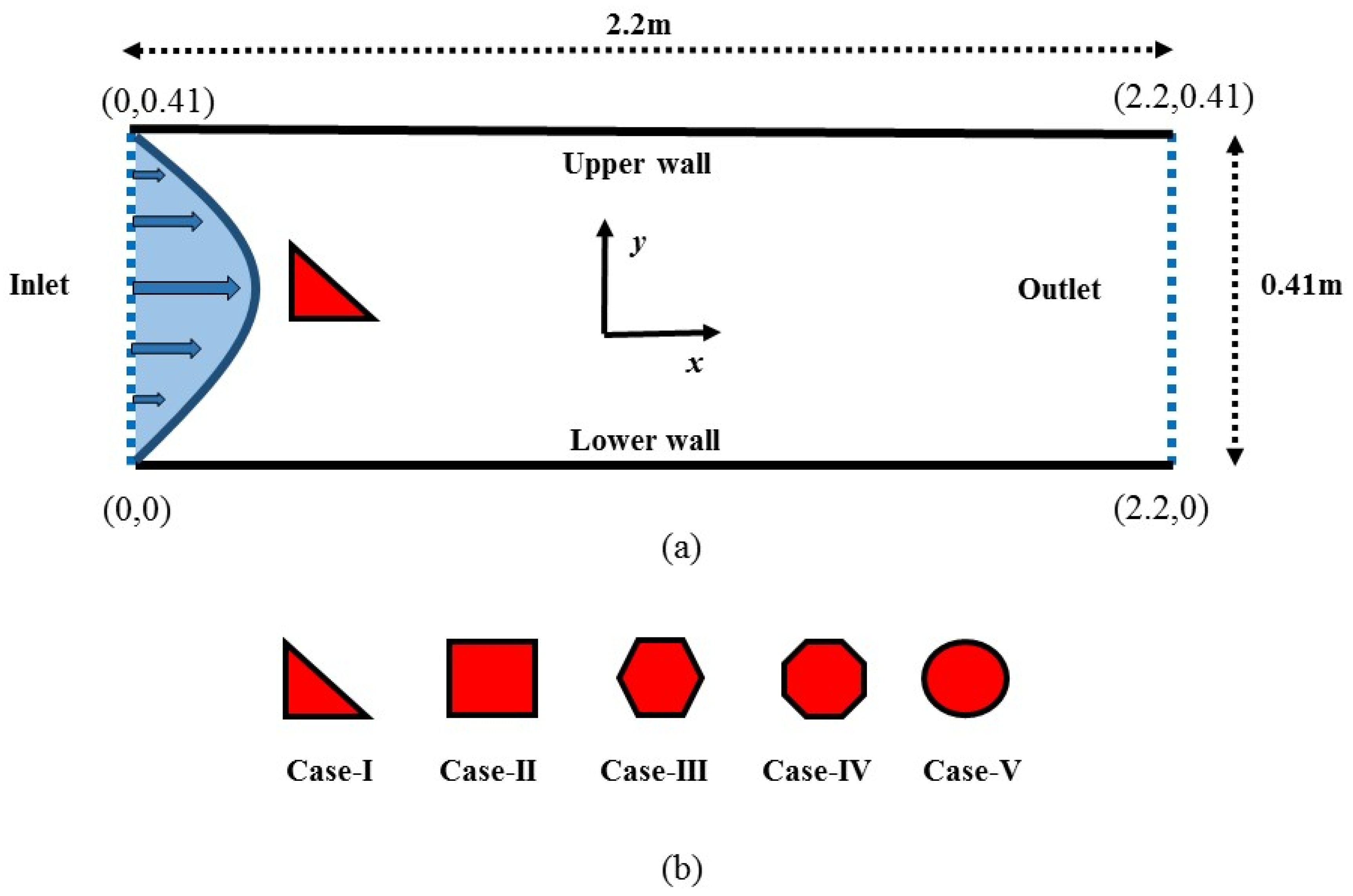
A rectangular channel is used to hold the laminar Newtonian fluid flow. A computational domain is a rectangular channel with a length of 2.2 m and a height of 0.41 m. The no-slip condition is considered at lower/upper walls. The right wall of the channel is subjected to the Neumann condition, whereas the left one is handled as in inlet. The linear velocity profile and the parabolic velocity distribution are included in the velocity presumption. The arriving fluid collides with obstructions in the channel. In this scheme, the circular-, octagon-, hexagon-, square-, and triangular-shaped cylinders are used as an impediment. The geometry of the problem is given in Figure 1a, and the installed obstacles are geometrically illustrated in Figure 1b.

3. Mathematical Formulation

Mathematical modeling is the best tool to study the laminar flow fields. For a better examination of the drag coefficient in corresponds to circular-, octagon-, hexagon-, square-, and triangular-shaped cylinders as obstructions we used mathematical modeling. To obtain to the final flow narrating differential equations, the continuity equation is reported as:

$$\frac{\partial \rho }{\partial t}+\overrightarrow{\nabla }\cdot (\rho \overrightarrow{\mathrm{V}})=0,$$

(1)

Thus, the momentum equation is as follows:

$$\rho \frac{D\overrightarrow{\mathrm{V}}}{Dt}=-\overrightarrow{\nabla }p+\mu {\overrightarrow{\nabla }}^2\overrightarrow{\mathrm{V}}+\rho \overrightarrow{B},$$

(2)

The following arrangement is used to obtain the dimensionless form of Equation (2):

$${\overrightarrow{\nabla }}^{*}=D_m\overrightarrow{\nabla }, p^{*}=p\frac{1}{\rho U_m{}^2}, {\overrightarrow{B}}^{*}=\overrightarrow{B}\frac{D_m}{U_m{}^2}, {\overrightarrow{\mathrm{V}}}^{*}(x,y,z,t)=\frac{\overrightarrow{\mathrm{V}}(x,y,z,t)}{U_m}, \frac{\partial }{\partial t^{*}}=\frac{D_m}{U_m}\frac{\partial }{\partial t},$$

(3)

Owning Equation (3), we have

$$\frac{D{\overrightarrow{\mathrm{V}}}^{*}}{D{t}^{*}}=-{\overrightarrow{\nabla }}^{*}{p}^{*}+\frac{\mu }{\rho D_m{U}_m} {\overrightarrow{\nabla }}^{*}{}^2{\overrightarrow{\mathrm{V}}}^{*}+{\overrightarrow{B}}^{*},$$

(4)

Equation (4) without “*” can be read as

$$\frac{D\overrightarrow{\mathrm{V}}}{Dt}=-\overrightarrow{\nabla }p+\frac{1}{\mathrm{Re}}{\overrightarrow{\nabla }}^2\overrightarrow{\mathrm{V}}+\overrightarrow{B},$$

(5)

where $\mu$ is viscosity, $\mathrm{Re}=\frac{\rho D_m{U}_m}{\mu }$ is Reynolds number, $\rho$ is fluid density, $\overrightarrow{B}$ is the body force, $U_m$ is the reference velocity, and $D_m$ is the characteristic length. By considering the following assumptions, namely time independent flow, two dimensional flow, and incompressible flow, the above-reported differential equations reduce to

$$\frac{\partial u}{\partial x}+\frac{\partial v}{\partial y}=0,$$

(6)

$$\mathrm{Re}\left(u\frac{\partial u}{\partial x}+v\frac{\partial u}{\partial y}\right)=-\mathrm{Re}\frac{\partial p}{\partial x}+\frac{{\partial }^{2}u}{\partial x^2}+\frac{{\partial }^{2}u}{\partial y^2},$$

(7)

$$\mathrm{Re}\left(u\frac{\partial v}{\partial x}+v\frac{\partial v}{\partial y}\right)=-\mathrm{Re}\frac{\partial p}{\partial y}+\frac{{\partial }^{2}v}{\partial x^2}+\frac{{\partial }^{2}v}{\partial y^2}.$$

(8)

For a linear velocity profile (LVP), the endpoint condition is expressed as:

$$\begin{array}{l}\mathrm{Left} \mathrm{wall} v=0,u=U_c,\\ \mathrm{Right} \mathrm{wall} \frac{\partial v}{\partial x}=\frac{\partial u}{\partial x}=0, \\ \mathrm{Other} \mathrm{walls} v=0, u=0.\end{array}$$

(9)

For parabolic velocity profile (PVP), the endpoint assumptions are:

$$\begin{array}{l}\mathrm{Left} \mathrm{wall} u=4. U_{Max} \left(H-y\right).y, v=0,\\ \mathrm{Right} \mathrm{wall} \frac{\partial v}{\partial x}=\frac{\partial u}{\partial x}=0, \\ \mathrm{Other} \mathrm{walls} v=0, u=0.\end{array}$$

(10)

The laminar fluid flow is considered with fully developed parabolic inflow velocity. It is normal to the inlet plane. Further, the $U_{Max}$ is maximum value of inlet velocity, and H is the height of the channel. One should note that the choice of parabolic profile is a more realistic approach [32] in evaluation with a linear velocity profile. In the present analysis, we consider both profiles for the sake of comparative study. The drag force is produced by the laminar fluid flow around an obstruction. It all comes down to the spot of obstructions in fluid because the drag force existence does not imply the presence of a lift force. The dimensionless drag and lift coefficients are more interesting than the drag and lift forces. Drag and lift coefficients are used to model all of the intricate relationships between shape, angle of attack, and flow conditions. We are interested to predict the drag force values as a drag coefficient by using artificial neural networking. Therefore, the mathematical relations toward lift and drag coefficients [32,33,34,35] are reported as follows:

$$L_f=\frac{2 L_F}{\rho {(U_{\mathrm{mean}})}^2{D}_m},$$

(11)

$$D_f=\frac{2 D_F}{\rho {(U_{\mathrm{mean}})}^2{D}_m}.$$

(12)

Otto Lilienthal was the first to apply a type of dimensionless coefficient in equations for lift and drag, but Ludwig Prandtl was the one who created the lift coefficient in its current form, and his work was the first to be published in 1923 [36,37]. The lift coefficient, was at first only pertained to fixed wings but was later expanded to fixed obstacles [38,39]. In our scenario, it is important to keep in mind that the presence of lift force is heavily dependent on the positioning of obstacles. For example, since we chose a channel with a height of 0.41 m, the obstruction should be slightly offset from the center (0.2,0.2) m. In this way, we would have the lift coefficient corresponding to the lift force. Additionally, if the obstruction is positioned at (0.2,0.2), and the channel height is set at 0.4 m, the fluid flow bifurcation will be sufficiently symmetric to eliminate the possibility of lift coefficient.

4. Artificial Neural Networking Design

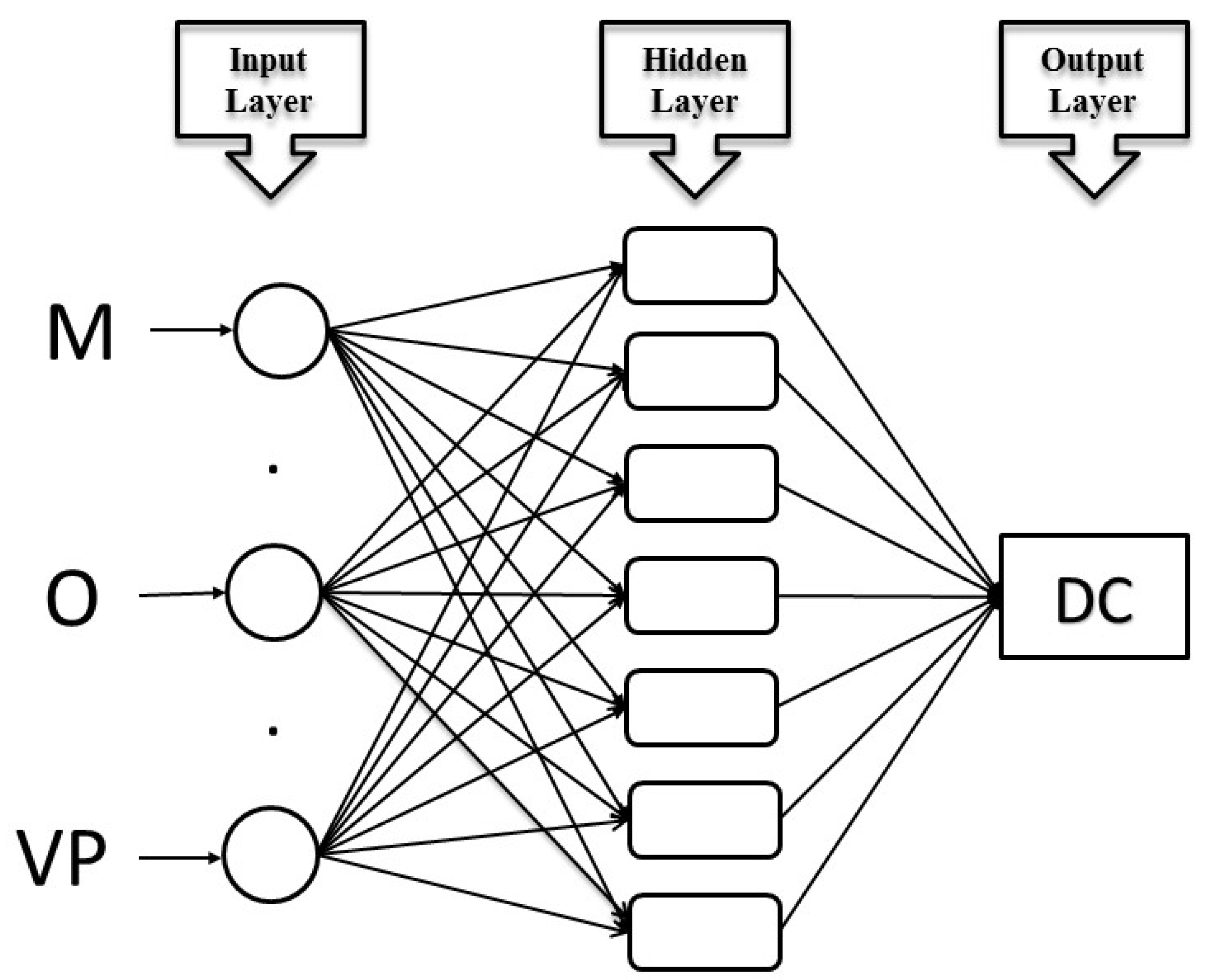
The ANN model is developed to analyze the hydrodynamic forces depending on the object for five different obstacles placed in a rectangular channel having laminar fluid flow. In the design of the ANN model, the back propagation (BP), feed forward (FF), multilayer perceptron (MLP) network model, which has high prediction accuracy with its strong structure, was preferred [40,41,42,43]. MLP basically consists of three main layers. The MLP network’s first layer is called the input layer, and at this layer, the data necessary for training are entered into the system. The second layer is the hidden layer, and it is important to note that at least one hidden layer exists for MLP. The next layer after the hidden layer is the output layer, and the network model outputs are found in the output layer. In input layer, three different input parameters are defined in this study. The first parameter is the meshing level (M), which has nine distinct values. At the second parameter, the values of obstacle (O) are defined. Five different architectures, namely circular-, octagon-, hexagon-, square-, and triangular-shaped, were considered as obstacle values. The third parameter defined in the input layer is the inlet velocity profiles (VP).

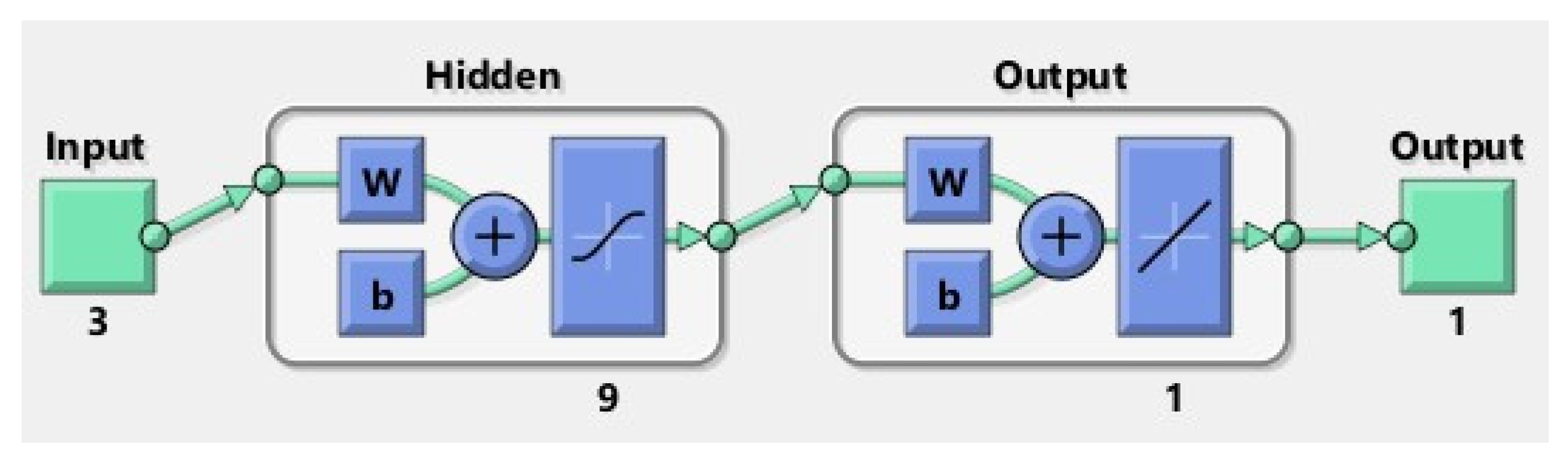
As inlet velocity profiles, two different profiles, linear and parabolic profiles, were carried. The drag coefficient (DC) value was obtained in the output layer of the MLP, which was developed by defining three different parameters in the input layer. Figure 2 offers the formation structure of the MLP neural network designed for estimating the DC values. The neuron [44] as a computational element exists in the hidden layer of MLP. Determining the number of neurons is one of the main challenges. The reason for this difficulty is that there is no fixed rule subject to strength of neurons [45,46]. In order to overcome this difficulty, the performance of the network models established with various neuron numbers is evaluated, and the optimum number of neurons is reached [47]. The same method was used in the designed model with nine neurons towards the hidden layer. For the model [48] prediction accuracy, optimizing the grouping of the data set utilized for training the ANN model is important. The model, which is frequently used in the literature, was used in grouping the data reserved for the training, validation, and testing stages of the model [49,50,51]. Here, 62 of the datapoints were utilized in the ANN model and trained by 90 datapoints; both testing and validation used 14. Figure 3 illustrates the structure of the ANN model.

Training algorithm with named Levenberg–Marquardt holds high training and learning performance, is used in the ANN model [52,53]. Pureline and Tan-Sig transfer functions are considered in output and hidden layers. Mathematical relationships [54,55] in this direction are given as:

$$f(x)=\frac{1}{e^{-x}+1},$$

(13)

Pureline(x) = x.

(14)

To verify the training and learning reliability of the models is an important task while designing the ANN models. Reliable completion of the learning phase of the model is also the main indicator of prediction reliability. Performance parameters were chosen in order to evaluate the training and learning stages [56]. The mathematical relationships [57,58] used in calculating the coefficient of determination (R) parameters and mean squared error (MSE) are reported as

$$MSE=\frac{1}{N}{\displaystyle \sum _{i=1}^N{(X_{\mathrm{targ}(i)}-X_{\mathrm{ANN}(i)})}^2}.$$

(15)

$$R=\sqrt{1-\frac{{\displaystyle \sum _{i=1}^N{(X_{\mathrm{targ}(i)}-X_{\mathrm{ANN}(i)})}^2}}{{\displaystyle \sum _{i=1}^N{(X_{\mathrm{targ}(i)})}^2}}},$$

(16)

Another method used together with performance parameters in examining the learning reliability and training of ANN models is to evaluate the deviation between network model outputs and the target information. The margin of deviation (MoD), which expresses the proportional deviation between the target and output values, is obtained using the following equation [59]:

$$\mathrm{MoD}(\%)=\left[\frac{X_{\mathrm{targ}}-X_{\mathrm{ANN}}}{X_{\mathrm{targ}}}\right]\times 100.$$

(17)

5. Results Analysis

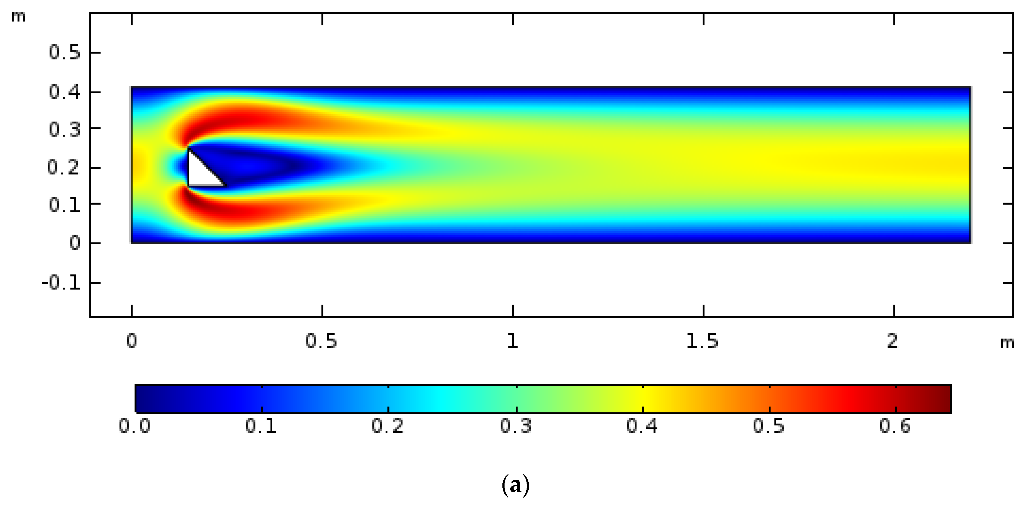
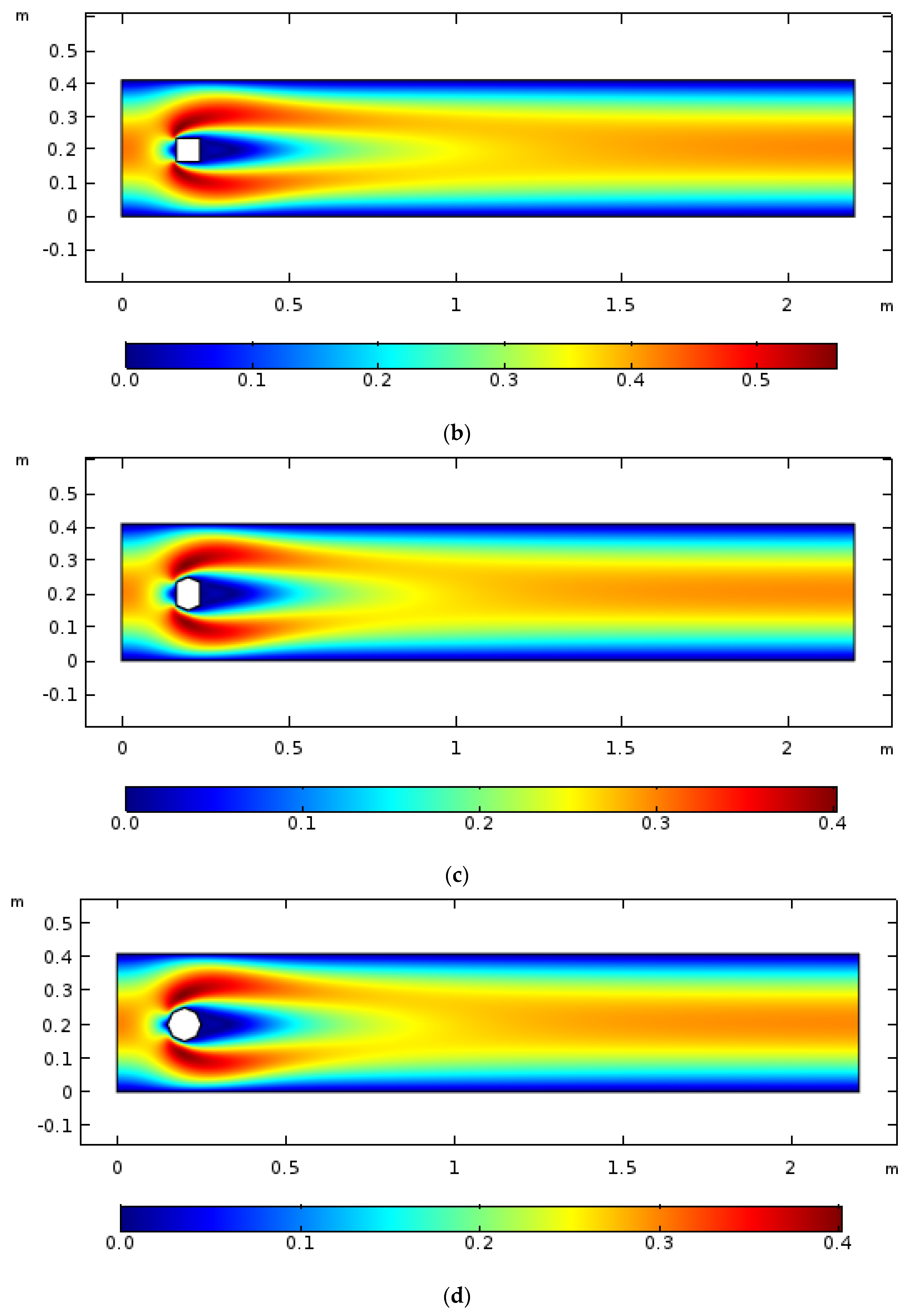
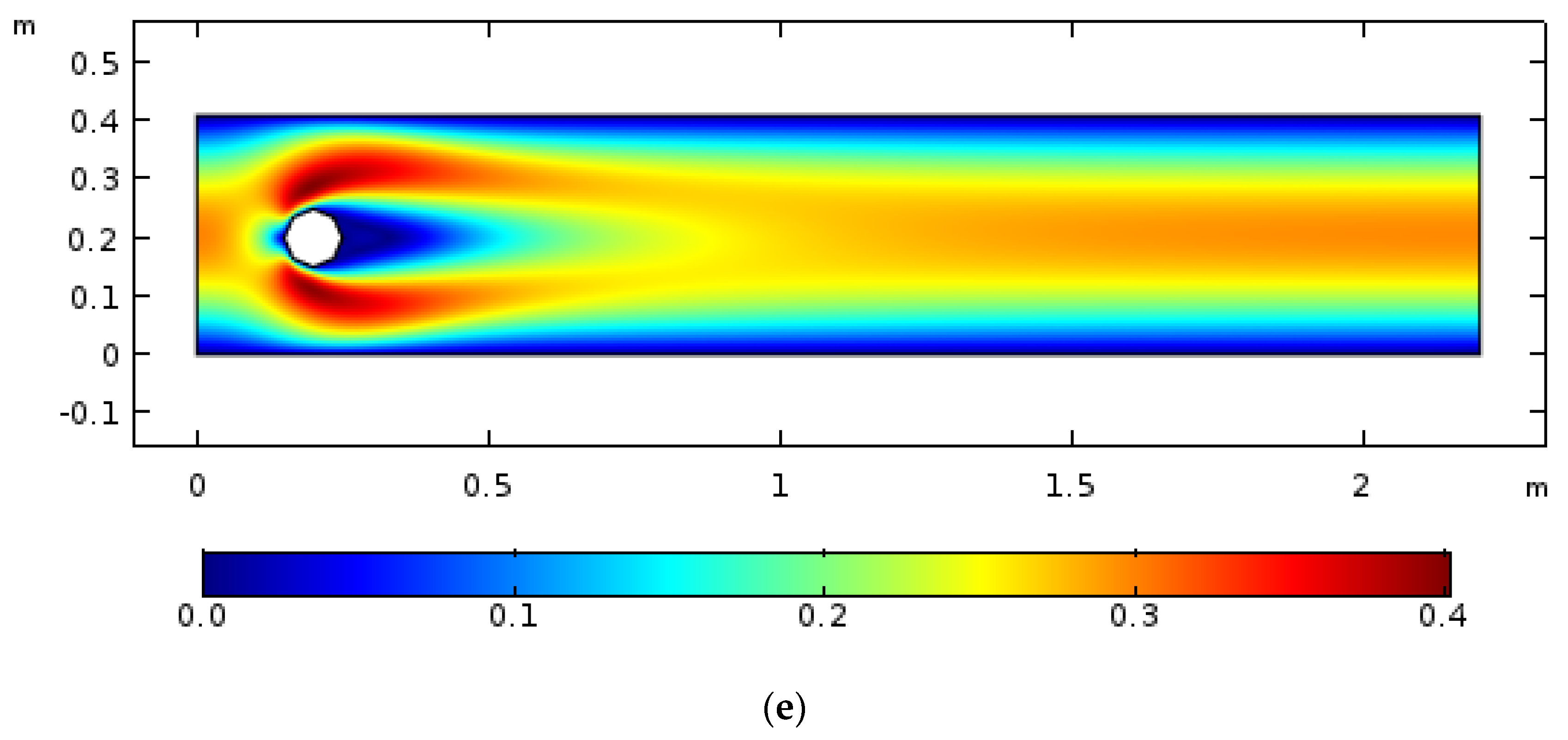
We considered five different cases subject to installation of regular obstacles. In Case-I, a triangular-shaped cylinder is installed in a rectangular channel with vertices (0.165, 0.165), (0.235, 0.165), and (0.165, 0.235). Installation of a square-shaped cylinder with vertices (0.165, 0.235), (0.165, 0.165), (0.235, 0.165), and (0.235, 0.235) is considered as Case-II. In Case-III, the hexagon-shaped cylinder is installed in the rectangular channel with vertices (0.2, 0.25), (0.165, 0.235), (0.165, 0.165), (0.2, 0.15), (0.235, 0.165), and (0.235, 0.235). The installation of an octagon-shaped cylinder with vertices (0.2, 0.25), (0.165, 0.235), (0.15, 0.2), (0.165, 0.165), (0.2, 0.15), (0.235, 0.165), (0.25, 0.2), and (0.235, 0.235) is considered as Case-IV. In Case-V, the circular shaped cylinder is installed in rectangular channel with a radius 0.05 m at the center (0.2, 0.2) m. The finite element approach is used to solve Equations (6)–(10) for assumption, namely parabolic velocity profile. The fluid flow visualization around triangular-, square-, hexagon-, octagon-, and circular-shaped cylinders is offered as Figure 4a–e, respectively.

Our goal is to have assessment of drag force in term of drag coefficient and to offer an artificial neural networking model for each case. The fundamentals subject to use of ANN model can be assessed in refs. [60,61,62]. In this regard, the hybrid meshing is used to get the numerical values of drag coefficient. Such values are obtained by doing line integration around each obstructions, namely circular-, octagon-, hexagon-, square-, and triangular-shaped cylinders.

Nine various meshing levels (1–9) are utilized for better approximation of drag coefficient. The values of drag coefficient are evaluated by using relationships given in Equation (12).

Table 1. Drag coefficient data for Case-I with LVP.

Mesh Level	Drag Coefficient
1	3.1750
2	3.1096
3	3.0436
4	2.9753
5	2.9572
6	2.9449
7	2.9319
8	2.9269
9	2.9253

,

Table 2. Drag coefficient data for Case-I with PVP.

Mesh Level	Drag Coefficient
1	6.3821
2	6.2656
3	6.1337
4	6.0820
5	6.0535
6	6.0361
7	6.0152
8	6.0080
9	6.0074

,

Table 3. Drag coefficient data for Case-II with LVP.

Mesh Level	Drag Coefficient
1	3.3490
2	3.2529
3	3.1646
4	3.1145
5	3.0958
6	3.0857
7	3.0743
8	3.0699
9	3.0686

,

Table 4. Drag coefficient data for Case-II with PVP.

Mesh Level	Drag Coefficient
1	4.0847
2	3.9819
3	3.8822
4	3.8374
5	3.8226
6	3.8127
7	3.7989
8	3.7950
9	3.7945

,

Table 5. Drag coefficient data for Case-III with LVP.

Mesh Level	Drag Coefficient
1	4.7449
2	4.7008
3	4.6374
4	4.5978
5	4.5882
6	4.5791
7	4.5696
8	4.5639
9	4.5619

,

Table 6. Drag coefficient data for Case-III with PVP.

Mesh Level	Drag Coefficient
1	5.4908
2	5.4549
3	5.3968
4	5.4002
5	5.4021
6	5.3983
7	5.3902
8	5.3851
9	5.3844

,

Table 7. Drag coefficient data for Case-IV with LVP.

Mesh Level	Drag Coefficient
1	5.1739
2	5.1376
3	4.6817
4	4.6266
5	4.5851
6	4.5683
7	4.5511
8	4.5394
9	4.5372

,

Table 8. Drag coefficient data for Case-IV with PVP.

Mesh Level	Drag Coefficient
1	5.8833
2	5.9483
3	5.4218
4	5.4066
5	5.3690
6	5.3618
7	5.3434
8	5.3299
9	5.3294

,

Table 9. Drag coefficient data for Case-V with LVP.

Mesh Level	Drag Coefficient
1	5.1671
2	4.8794
3	4.8317
4	4.8197
5	4.8014
6	4.8040
7	4.8005
8	4.7965
9	4.7944

and

Table 10. Drag coefficient data for Case-V with PVP.

Mesh Level	Drag Coefficient
1	6.0207
2	5.6119
3	5.5788
4	5.5796
5	5.5892
6	5.5930
7	5.5863
8	5.5812
9	5.5811

are plotted in this direction. Ref. [24] is the reference support subject to numerical data of drag coefficient. To be more specific, we considered five different obstacles, and hence, we have five different flow fields.

Table 1 and Table 2 offer the numerical values of the drag coefficient towards the triangular-shaped obstacle for both linear and parabolic profiles. Table 3 and Table 4 contain the values of the drag coefficient subject to the square-shaped obstacle for linear and parabolic profiles. The drag coefficient values towards the hexagon-shaped obstacle are summarized in Table 5 and Table 6. Table 7 and Table 8 present the numerical values of the drag coefficient towards the octagon-shaped obstacle for both linear and parabolic profiles.

Table 9 and Table 10 contains the values of drag coefficient subject to circular shaped obstacle for linear and parabolic profiles. In literature, Schäfer et al. [32] considered a rectangular channel of height 0.41 m and a length 2.2 m. They installed a circular-shaped cylinder as an obstruction. Newtonian fluid is considered at the inlet with a parabolic profile and proposed drag coefficient $C_D=5.579535$ and lift coefficient $C_L=0.010618$. The novelty of the present article includes drag coefficient evaluation and a corresponding neural network model for five various obstacles, namely triangular-, square-, hexagon-, octagon-, and circular-shaped cylinders. Besides, we compared the values of drag and lift coefficients with Schäfer et al. [32], and an excellent match was found, which yields the surety of the present attempt.

Table 11. Coefficient comparison with Schäfer et al. [32] at Re = 20.

Mesh Level	Lift Coefficient (Present Results)	Lift Coefficient (Schäfer et al. [32])	Drag Coefficient (Present Results)	Drag Coefficient (Schäfer et al. [32])
4	−0.06141	-	6.5651	-
5	−0.04346	-	6.2766	-
6	−0.03001	-	5.9710	-
7	0.02031	0.010618	5.5641	5.579535
8	0.01308	0.010618	5.5702	5.579535
9	0.01051	0.010618	5.5712	5.579535

is offered in this regard. In order to verify the ideal completion of the training phase, which was designed to analyze the hydrodynamic forces depending on the object, for five different obstacles placed in a rectangular channel in fluid flow, the training performance was examined in detail.

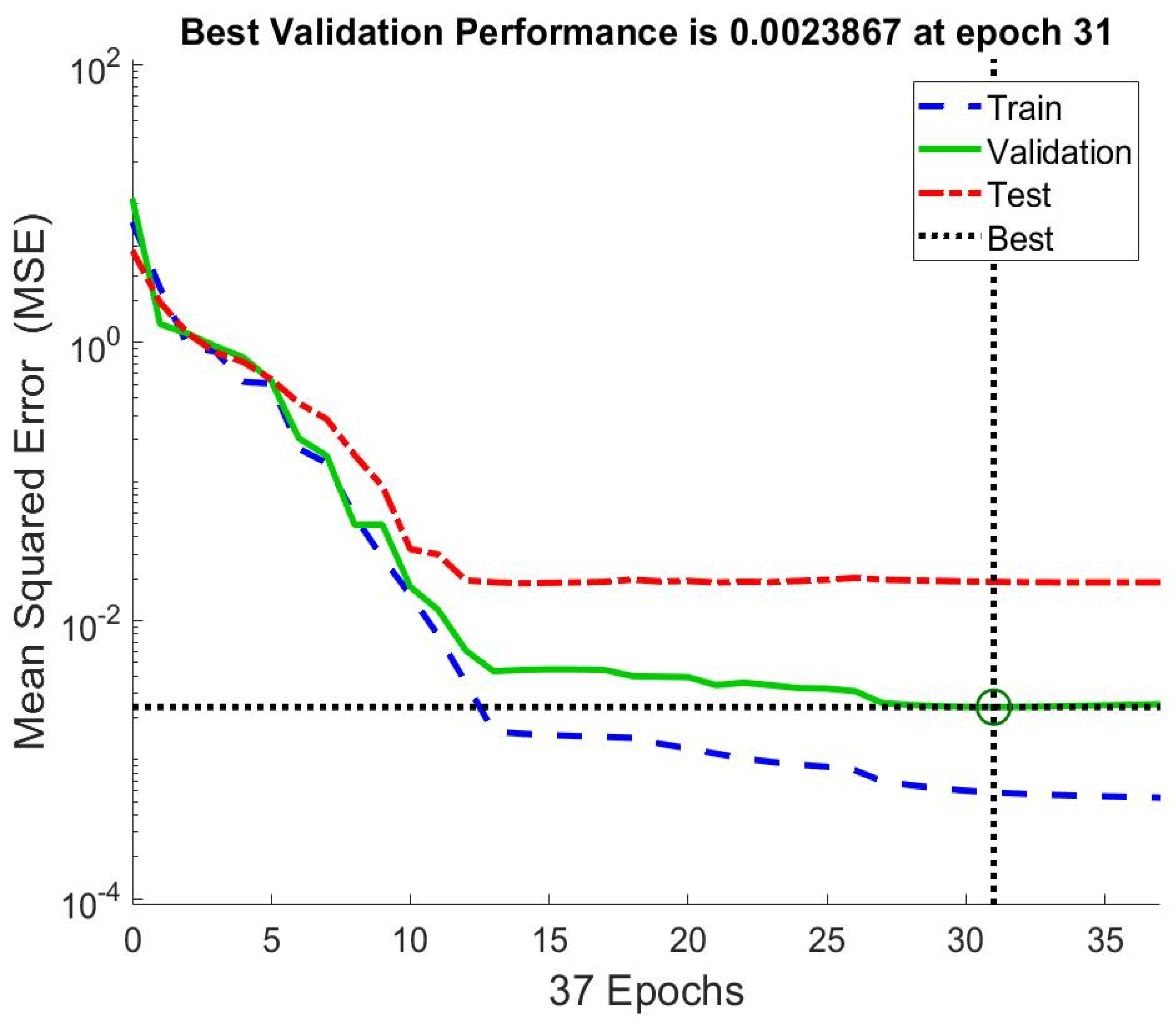
In Figure 5, the training performance graph of the MLP neural network model is presented. The figure shows the MSE values calculated for the testing, validation, and training events. For MLP network when the graph is examined, at start of training phase, the MSE values are observed higher and decrease towards developing epochs. The decreasing values of MSE subject to each epoch show that the error values are decreasing gradually. When the thirty-first epoch is reached, the best validation performance is achieved, and the training phase of the MLP neural network is terminated.

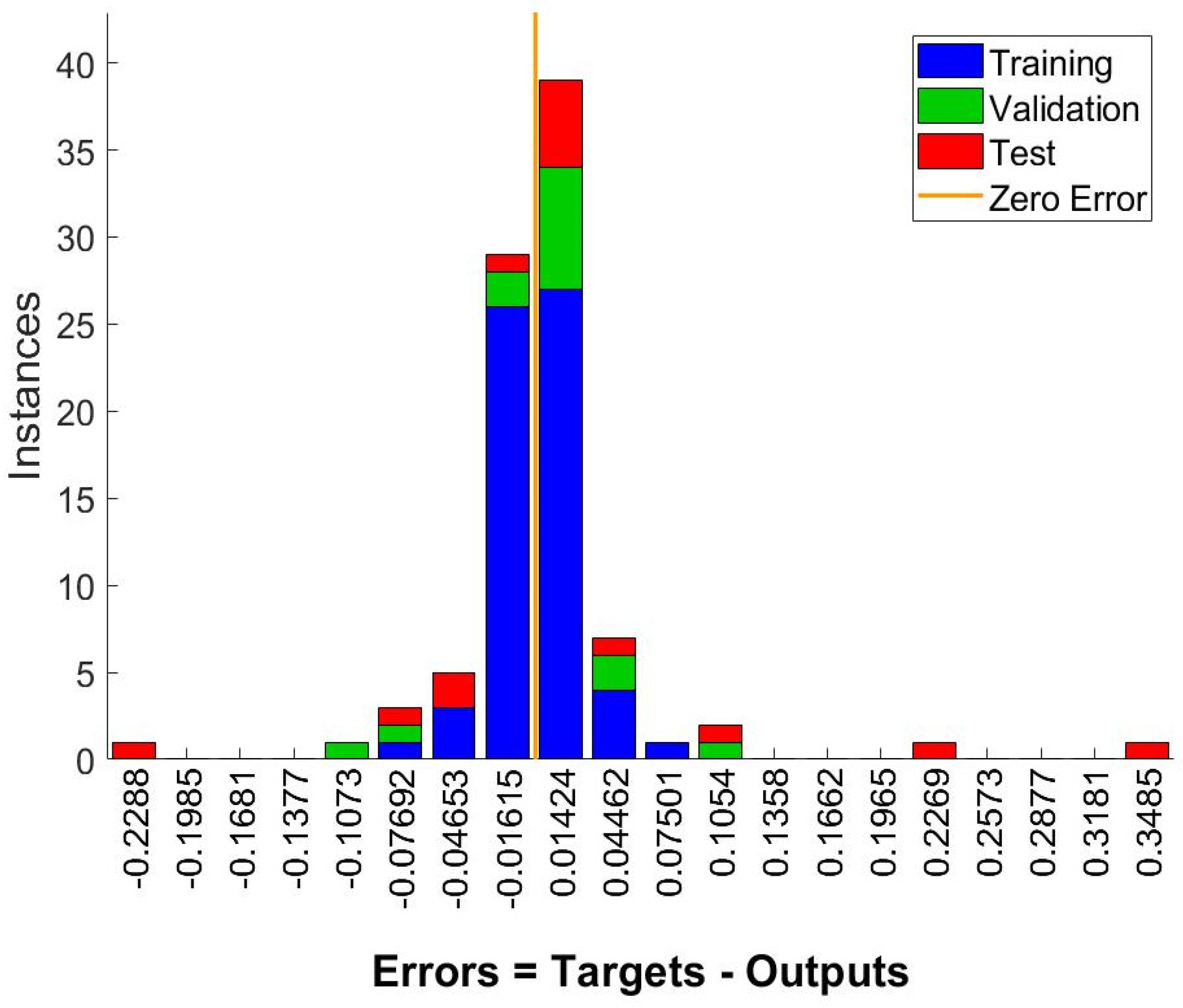
Findings from Figure 5 highlight the ideal completion of training phase and have low errors. Figure 6 shows the error histogram generated for the training phase of the ANN model. In the error histograms, the error values obtained during the training phase are presented, and it is aimed to perform the error analysis.

When the given error histogram is seen, we noticed the error values of the grouped data for the training, validation, and test stages are near the zero-error line. Errors values are sufficiently lessened. The results obtained from the analysis of the error histogram outlined the low-error completion of training phase.

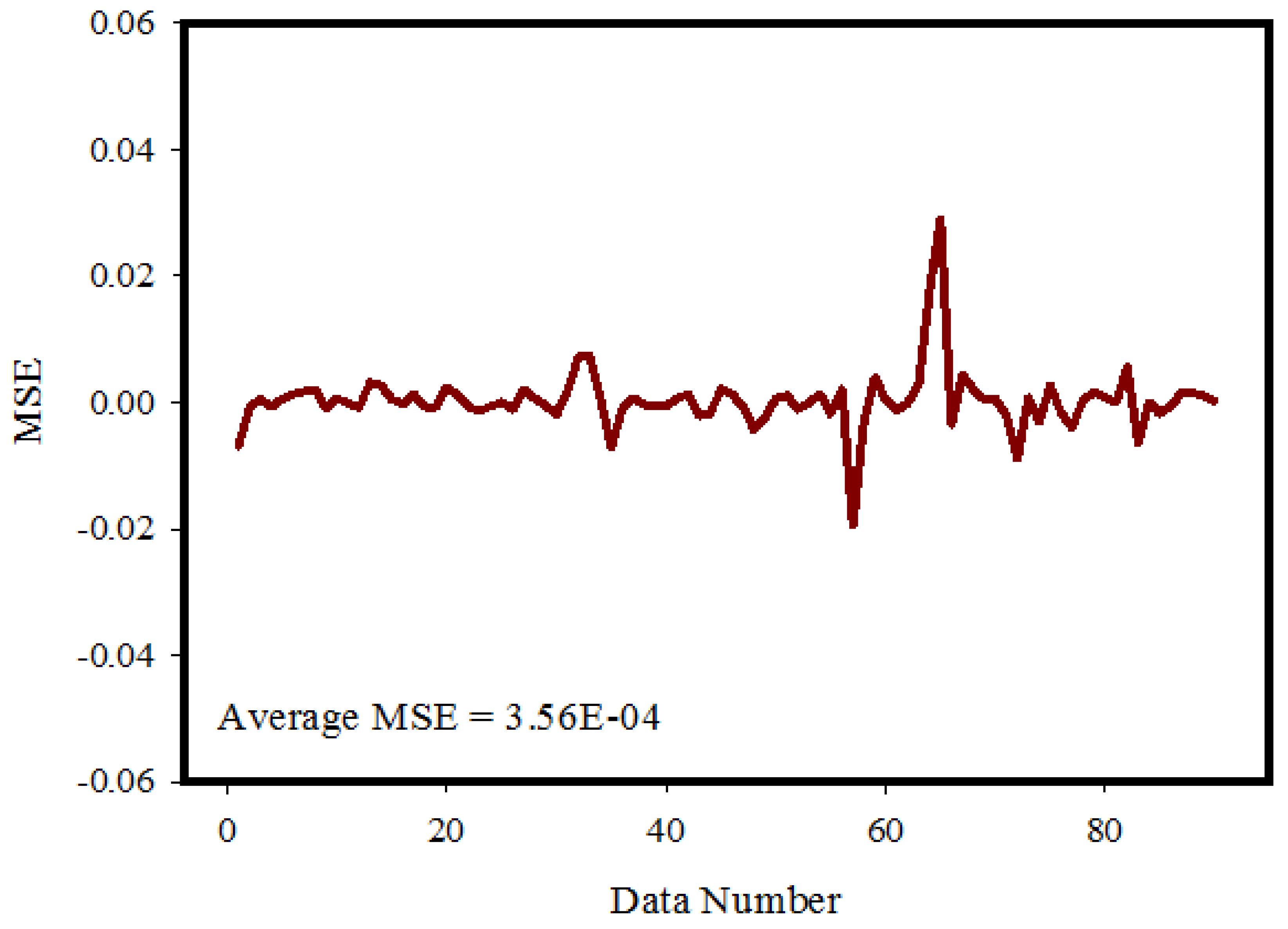
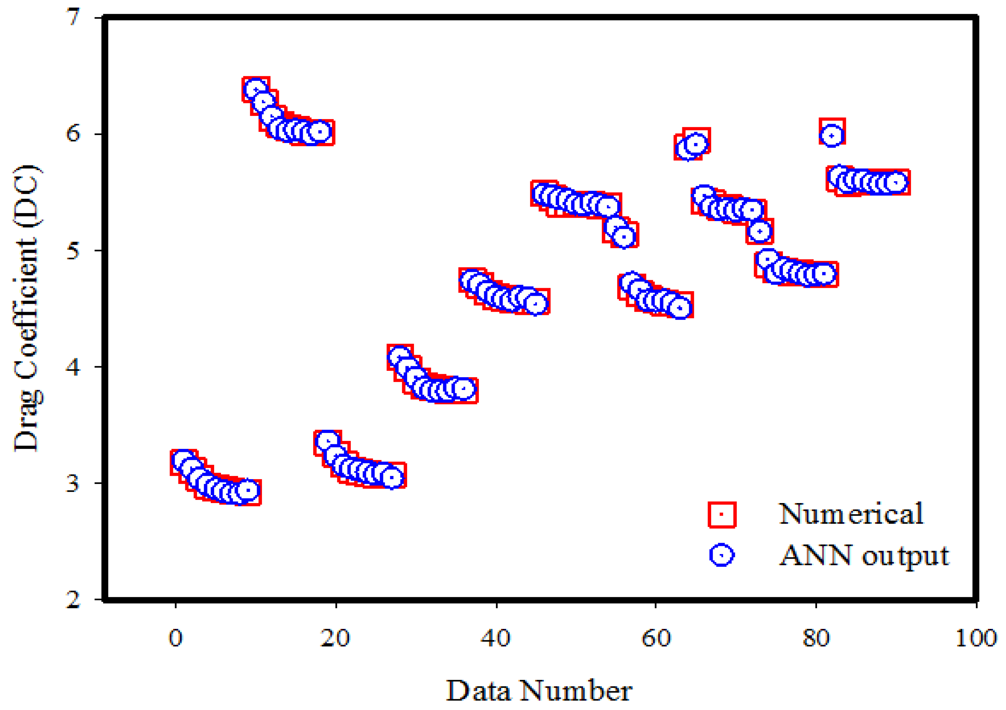
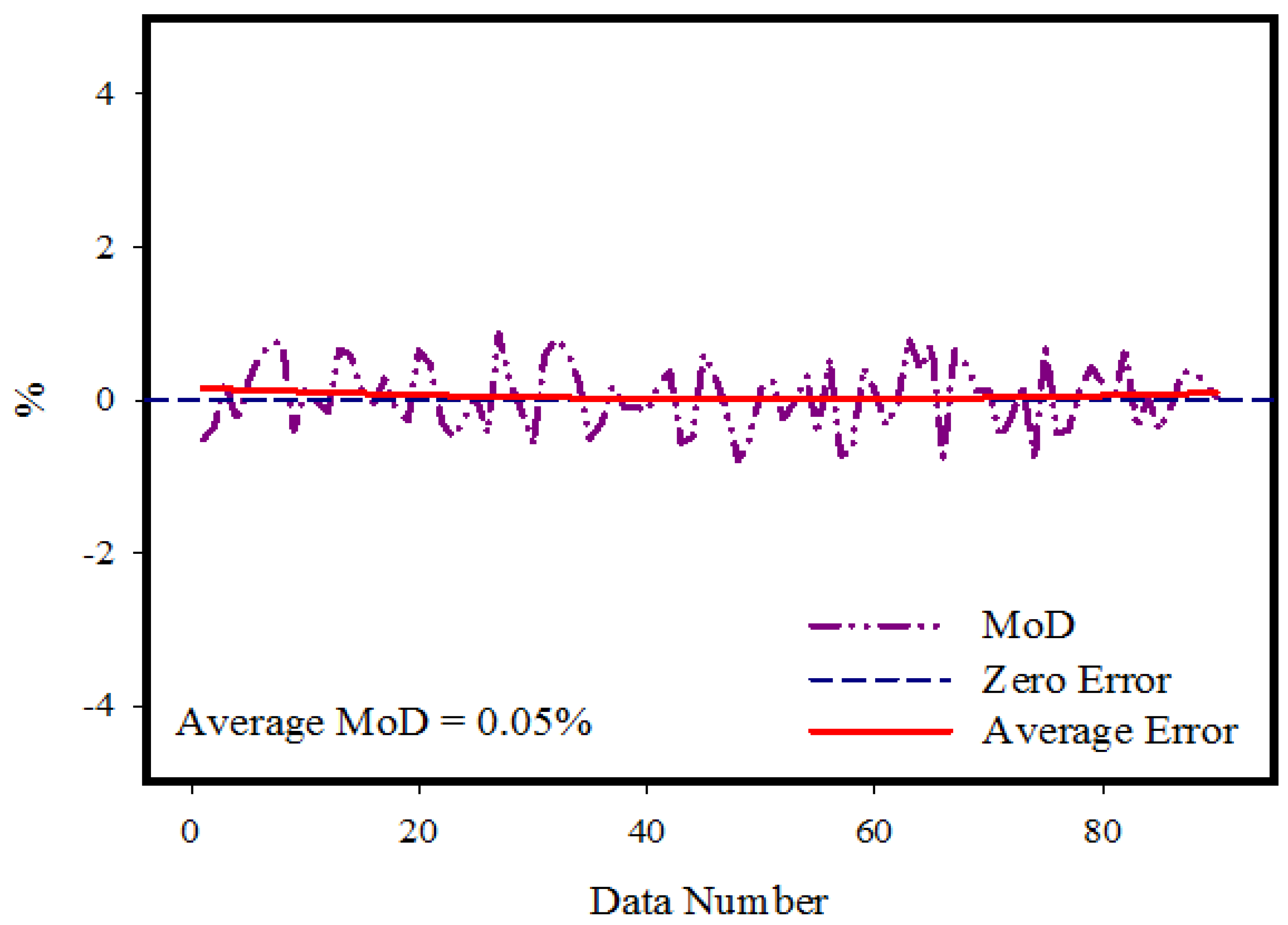
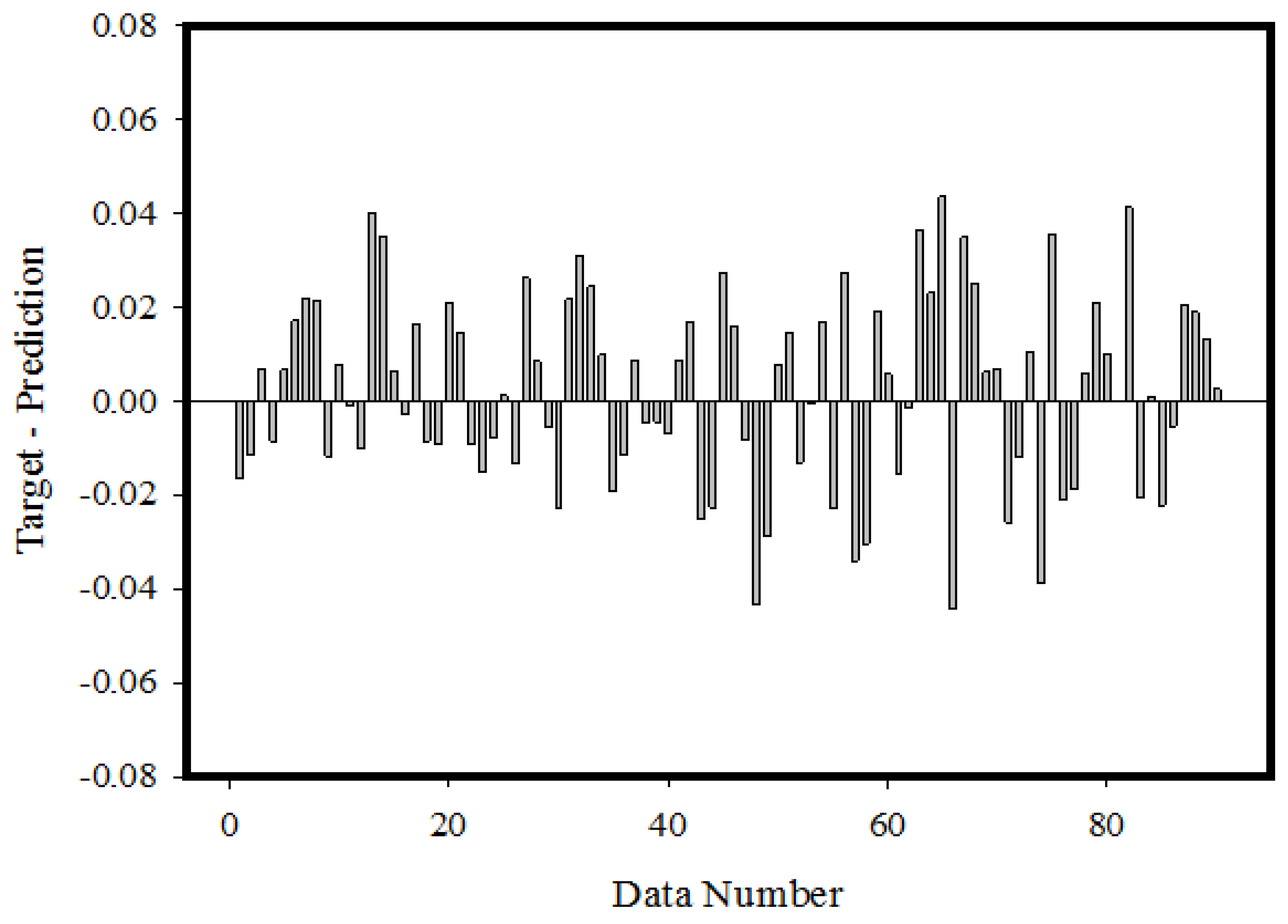
The values of MSE are approximated for each datapoint of the MLP neural network model developed with a total of 90 datasets and are shown in Figure 7. When the data line expressing the MSE outcomes calculated is examined, we observed that it is in a line close to the zero value in general. The MSE values proximity to zero implies that the error values received from the MLP neural network training phase are very low. The mean of MSE values calculated for 90 datapoints was obtained as 3.56 × 10⁻⁴. The results obtained from the MSE values clearly confirm that the training phase of the MLP neural network developed for the estimation of DC values has been ideally completed, and it has been designed to produce extremely accurate predictions. After the training and learning validation of the designed ANN model, the accuracy of the outputs obtained from the neural network was analyzed. Figure 8 shows the correspondence of the DC values obtained from the MLP neural network and the numerical data, which are the target values. By following Figure 8, it is observed that the outputs of the ANN model shown in blue are a great match with the target data shown in red. This perfect fit of the datapoints’ own DC values by way of designed ANN model are very close to the actual data, which are the target values. MoD values were calculated and examined in order to analyze the percentage difference between the ANN model predicted values and the goal values. Figure 9 shows the MoD values calculated for each of the 90 data values. Looking at the graph line expressing the MoD values, we noticed the datapoints are generally very close to the zero-error line. Such closeness of the MoD values indicates that the deviation of the predicted values from the target values is very low for each datapoint. We further observed that the average MoD value expressed with a red line is very similar to the zero-error line. The average MoD value calculated for all datapoints was obtained as 0.05%. The results obtained from the MoD data presented in Figure 9 showed that our ANN model has the capacity to predict DC values with less error. Figure 10 shows the disparities between the target values and the ANN outputs in order to perform a more detailed error analysis of the ANN model. When the calculated differences are analyzed, we noticed that the difference values between the target data and ANN outputs are very low.

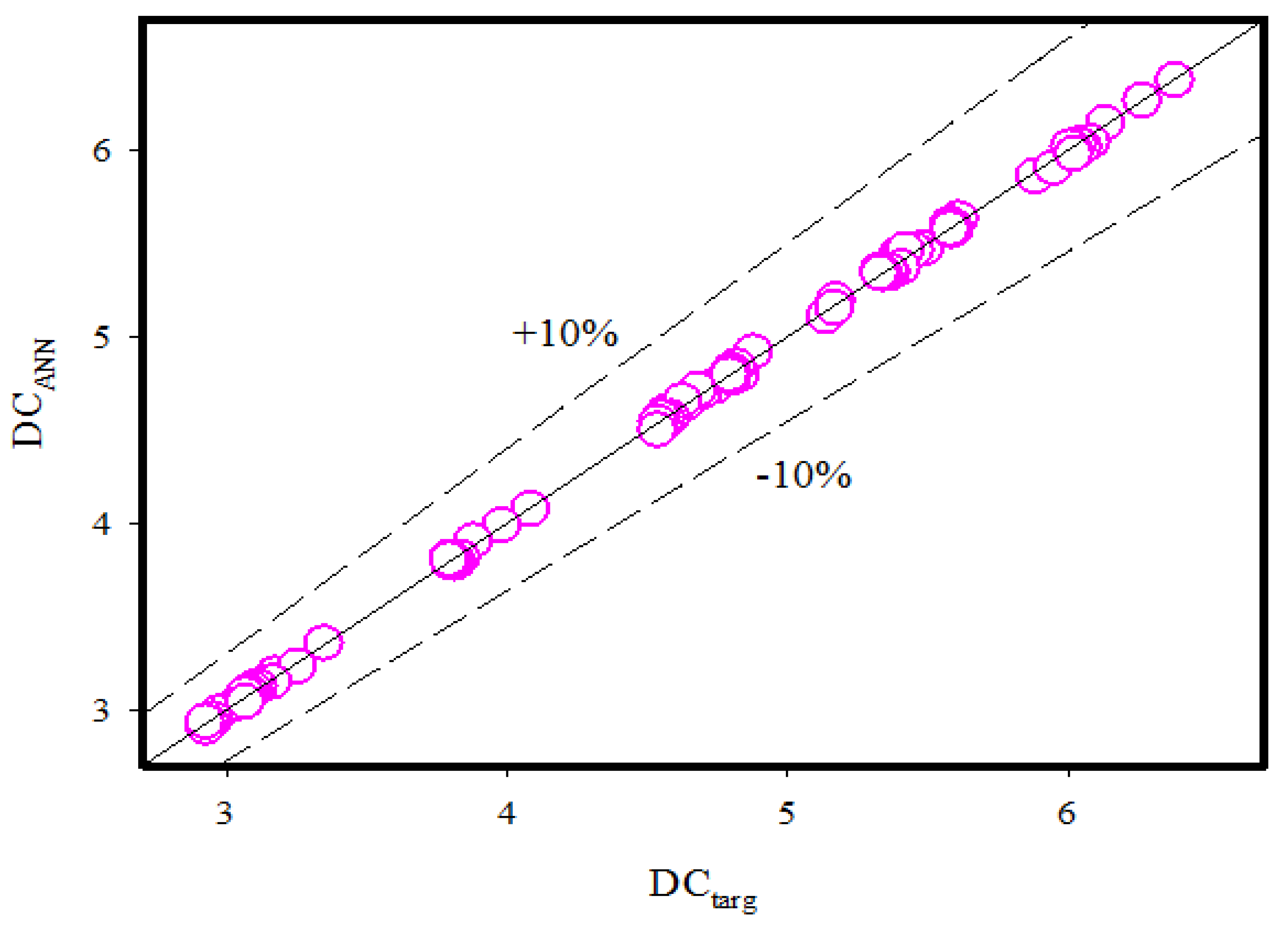
The fact that the differences between the output and target values obtained were very low, together with the MoD values, clearly confirms that the MLP network model is created to make predictions with less errors. The output and target values are shown on two axes of the same graph in order to see in more detail the agreement between the outputs obtained from the MLP network model and the target values. In Figure 11, the target values are on the x-axis, and the ANN outputs are on the y-axis. When the positions of the datapoints are examined, we noticed that each datapoint is located on the zero-error line. The datapoints, on the other hand, are within the ±10% error zone. The calculated R value for the developed MLP neural network was also found to be 0.99969. All these results clearly show that the developed ANN model is an ideal tool to be utilized for examination of the hydrodynamic forces depending on the object for five different obstacles placed in a rectangular channel having laminar fluid flow, and it has been developed to predict DC values with very high accuracy. Collectively, the drag coefficient corresponding to various obstacles in rectangular channel is object-dependent. In this regard, the development of an artificial neural network model for an optimum path from a triangle to a circular obstacle may provide benchmarks for subsequent research to extend the examination for the hydrodynamic forces and stable individualities towards completely or partially submerged objects from an engineering standpoint.

6. Conclusions

The regular obstacles, namely circular, octagon, hexagon, square, and triangle, were placed in a rectangular channel having laminar fluid flow. As an outlet, the Neumann condition was applied to the right wall. On both walls, namely the lower and upper, the no-slip condition was maintained. The fluid flowed from the channel’s left wall using two different velocity profiles: linear velocity and parabolic velocity. The flow equations were solved using the finite element method, and the drag coefficient for each obstacle was calculated by taking into account both linear and parabolic profiles. The drag coefficient values were calculated by performing line integration around installed obstructions. Corresponding to such drag coefficient values, we developed an ANN model for drag force faced by various obstacles towards the flow of the liquid stream in a rectangular channel. The key outcomes in the context of developing the ANN model for hydrodynamic force are as follows:

• The best validation performance is achieved at the thirty-first epoch, and the training phase of the MLP neural network is terminated.
• The training phase of the designed MLP neural network is completed with very low errors.
• The MSE values proximity to zero implies that the error values received from the MLP neural network training phase are very low.
• The average MoD value calculated for all datapoints was obtained as 0.05%.
• The calculated R-value for the developed MLP neural network was also found to be 0.99969.

References

- Milewski, P.A.; Vanden-Broeck, J.M. Time dependent gravity-capillary flows past an obstacle. Wave Motion 1999, 29, 63–79. [Google Scholar] [CrossRef]
- Wen, X.; Manik, K. A boundary integral method for gravitational fluid flow over a semi-circular obstruction using an interpolative technique. Eng. Anal. Bound. Elem. 2000, 24, 31–41. [Google Scholar] [CrossRef]
- Chashechkin, Y.D.; Mitkin, V.V. Experimental study of a fine structure of 2D wakes and mixing past an obstacle in a continuously stratified fluid. Dyn. Atmos. Ocean. 2001, 34, 165–187. [Google Scholar] [CrossRef]
- Ogata, H.; Amano, K.; Sugihara, M.; Okano, D. A fundamental solution method for viscous flow problems with obstacles in a periodic array. J. Comput. Appl. Math. 2003, 152, 411–425. [Google Scholar] [CrossRef] [Green Version]
- Bogoyavlenskiy, V.A.; Giamis, A.C.; Cotts, E.J. Mean-field dynamics of free surface flows through obstacle arrays in a narrow passage: Amendments of the Washburn model. Fluid Dyn. Res. 2004, 35, 23. [Google Scholar] [CrossRef]
- Dollet, B.; Elias, F.; Quilliet, C.; Huillier, A.; Aubouy, M.; Graner, F. Two-dimensional flows of foam: Drag exerted on circular obstacles and dissipation. Colloids Surf. A Physicochem. Eng. Asp. 2005, 263, 101–110. [Google Scholar] [CrossRef] [Green Version]
- Ogata, H.; Amano, K. A fundamental solution method for three-dimensional viscous flow problems with obstacles in a periodic array. J. Comput. Appl. Math. 2006, 193, 302–318. [Google Scholar] [CrossRef] [Green Version]
- Varela, J.; Araújo, M.; Bove, I.; Cabeza, C.; Usera, G.; Martí, A.C.; Montagne, R.; Sarasúa, L.G. Sarasúa. Instabilities developed in stratified flows over pronounced obstacles. Phys. A Stat. Mech. Appl. 2007, 386, 681–685. [Google Scholar] [CrossRef]
- Pierotti, D.; Simioni, P. The steady two-dimensional flow over a rectangular obstacle lying on the bottom. J. Math. Anal. Appl. 2008, 342, 1467–1480. [Google Scholar] [CrossRef] [Green Version]
- Grigoriadis, D.G.E.; Kassinos, S.C. Lagrangian particle dispersion in turbulent flow over a wall mounted obstacle. Int. J. Heat Fluid Flow 2009, 30, 462–470. [Google Scholar] [CrossRef]
- Kenjereš, S.; Ten Cate, S.; Voesenek, C.J. Vortical structures and turbulent bursts behind magnetic obstacles in transitional flow regimes. Int. J. Heat Fluid Flow 2011, 32, 510–528. [Google Scholar] [CrossRef] [Green Version]
- Oztop, H.F.; Mushatet, K.S.; Yılmaz, İ. Analysis of turbulent flow and heat transfer over a double forward facing step with obstacles. Int. Commun. Heat Mass Transf. 2012, 39, 1395–1403. [Google Scholar] [CrossRef]
- Zhang, X.; Huang, H. Effect of magnetic obstacle on fluid flow and heat transfer in a rectangular duct. Int. Commun. Heat Mass Transf. 2014, 51, 31–38. [Google Scholar] [CrossRef]
- Chatterjee, D.; Mondal, B. Control of flow separation around bluff obstacles by superimposed thermal buoyancy. Int. J. Heat Mass Transf. 2014, 72, 128–138. [Google Scholar] [CrossRef]
- Tanase, A.; Groeneveld, D.C. An experimental investigation on the effects of flow obstacles on single phase heat transfer. Nucl. Eng. Des. 2015, 288, 195–207. [Google Scholar] [CrossRef]
- Bera, S.; Bhattacharyya, S. Electroosmotic flow in the vicinity of a conducting obstacle mounted on the surface of a wide microchannel. Int. J. Eng. Sci. 2015, 94, 128–138. [Google Scholar] [CrossRef]
- Dbouk, T. A suspension balance direct-forcing immersed boundary model for wet granular flows over obstacles. J. Non-Newton. Fluid Mech. 2016, 230, 68–79. [Google Scholar] [CrossRef]
- Rashidi, S.; Bovand, M.; Esfahani, J.A. Opposition of Magnetohydrodynamic and AL2O3–water nanofluid flow around a vertex facing triangular obstacle. J. Mol. Liq. 2016, 215, 276–284. [Google Scholar] [CrossRef]
- Eter, A.; Groeneveld, D.; Tavoularis, S. Convective heat transfer in supercritical flows of CO2 in tubes with and without flow obstacles. Nucl. Eng. Des. 2017, 313, 162–176. [Google Scholar] [CrossRef]
- Barman, A.; Dash, S.K. Effect of obstacle positions for turbulent forced convection heat transfer and fluid flow over a double forward facing step. Int. J. Therm. Sci. 2018, 134, 116–128. [Google Scholar] [CrossRef]
- Issakhov, A.; Zhandaulet, Y.; Nogaeva, A. Numerical simulation of dam break flow for various forms of the obstacle by VOF method. Int. J. Multiph. Flow 2018, 109, 191–206. [Google Scholar] [CrossRef]
- Singh, R.J.; Gohil, T.B. Numerical study of MHD mixed convection flow over a diamond-shaped obstacle using OpenFOAM. Int. J. Therm. Sci. 2019, 146, 106096. [Google Scholar] [CrossRef]
- Torregrosa, A.; Gil, A.; Quintero, P.; Ammirati, A.; Denayer, H.; Desmet, W. Prediction of flow induced vibration of a flat plate located after a bluff wall mounted obstacle. J. Wind Eng. Ind. Aerodyn. 2019, 190, 23–39. [Google Scholar] [CrossRef]
- Rehman, K.U. Object dependent optimization of hydrodynamic forces in liquid stream: Finite element analysis. J. Mol. Liq. 2020, 298, 111953. [Google Scholar] [CrossRef]
- Yang, S.; Wang, X.; Liu, Q.; Pan, M. Numerical simulation of fast granular flow facing obstacles on steep terrains. J. Fluids Struct. 2020, 99, 103162. [Google Scholar] [CrossRef]
- Abdelmalek, Z.; Rehman, K.U.; Tlili, I. Grooved domain magnetized optimization (GDMO) of hydrodynamic forces due to purely viscous flowing liquid stream: A computational study. J. Mol. Liq. 2020, 304, 112766. [Google Scholar] [CrossRef]
- Tas-Koehler, S.; Liao, Y.; Hampel, U. A critical analysis of drag force modelling for disperse gas-liquid flow in a pipe with an obstacle. Chem. Eng. Sci. 2021, 246, 117007. [Google Scholar] [CrossRef]
- Lin, S.; Liu, J.; Xia, H.; Zhang, Z.; Ao, X. A numerical study of particle-laden flow around an obstacle: Flow evolution and Stokes number effects. Appl. Math. Model. 2022, 103, 287–307. [Google Scholar] [CrossRef]
- John, V. Reference values for drag and lift of a two-dimensional time-dependent flow around a cylinder. Int. J. Numer. Methods Fluids 2004, 44, 777–788. [Google Scholar] [CrossRef]
- Rajani, B.N.; Kandasamy, A.; Majumdar, S. Numerical simulation of laminar flow past a circular cylinder. Appl. Math. Model. 2009, 33, 1228–1247. [Google Scholar] [CrossRef]
- Syrakos, A.; Georgiou, G.C.; Alexandrou, A.N. Thixotropic flow past a cylinder. J. Non-Newton. Fluid Mech. 2015, 220, 44–56. [Google Scholar] [CrossRef] [Green Version]
- Schäfer, M.; Turek, S.; Durst, F.; Krause, E.; Rannacher, R. Benchmark computations of laminar flow around a cylinder. In Flow Simulation with High-Performance Computers II; Vieweg + Teubner Verlag: Wiesbaden, Germany, 1996; pp. 547–566. [Google Scholar]
- Yuce, M.I.; Kareem, D.A. A numerical analysis of fluid flow around circular and square cylinders. J. Am. Water Work. Assoc. 2016, 108, E546–E554. [Google Scholar] [CrossRef]
- Robertson, F.H.; Lane-Serff, G.F. Drag on pairs of square section obstacles in free-surface flows. Phys. Rev. Fluids 2018, 3, 123802. [Google Scholar] [CrossRef] [Green Version]
- Mahmood, R.; Hussain Majeed, A.; Ain, Q.U.; Awrejcewicz, J.; Siddique, I.; Shahzad, H. Computational Analysis of Fluid Forces on an Obstacle in a Channel Driven Cavity: Viscoplastic Material Based Characteristics. Materials 2022, 15, 529. [Google Scholar] [CrossRef]
- Bishop, R.E.D.; Hassan, A.Y. The lift and drag forces on a circular cylinder in a flowing fluid. In Proceedings of the Royal Society of London. Series A. Mathematical and Physical Sciences; Royal Society: London, UK, 1964; Volume 277, pp. 32–50. [Google Scholar]
- Burgers, P.; Alexander, D.E. Normalized lift: An energy interpretation of the lift coefficient simplifies comparisons of the lifting ability of rotating and flapping surfaces. PLoS ONE 2012, 7, e36732. [Google Scholar] [CrossRef] [Green Version]
- Jester, W.; Kallinderis, Y. Numerical study of incompressible flow about fixed cylinder pairs. J. Fluids Struct. 2003, 17, 561–577. [Google Scholar] [CrossRef]
- Baranyi, L. Computation of unsteady momentum and heat transfer from a fixed circular cylinder in laminar flow. J. Comput. Appl. Mech. 2003, 4, 13–25. [Google Scholar]
- Vaferi, B.; Eslamloueyan, R.; Ayatollahi, S. Automatic recognition of oil reservoir models from well testing data by using multi-layer perceptron networks. J. Pet. Sci. Eng. 2011, 77, 254–262. [Google Scholar] [CrossRef]
- Canakci, A.; Ozsahin, S.; Varol, T. Modeling the influence of a process control agent on the properties of metal matrix composite powders using artificial neural networks. Powder Technol. 2012, 228, 26–35. [Google Scholar] [CrossRef]
- Vaferi, B.; Samimi, F.; Pakgohar, E.; Mowla, D. Artificial neural network approach for prediction of thermal behavior of nanofluids flowing through circular tubes. Powder Technol. 2014, 267, 1–10. [Google Scholar] [CrossRef]
- Çolak, A.B. Developing optimal artificial neural network (ANN) to predict the specific heat of water based yttrium oxide (Y2O3) nanofluid according to the experimental data and proposing new correlation. Heat Transf. Res. 2020, 51, 1565–1586. [Google Scholar] [CrossRef]
- Ahmadloo, E.; Azizi, S. Prediction of thermal conductivity of various nanofluids using artificial neural network. Int. Commun. Heat Mass Transf. 2016, 74, 69–75. [Google Scholar] [CrossRef]
- Bonakdari, H.; Zaji, A.H. Open channel junction velocity prediction by using a hybrid self-neuron adjustable artificial neural network. Flow Meas. Instrum. 2016, 49, 46–51. [Google Scholar] [CrossRef]
- Çolak, A.B.; Güzel, T.; Yıldız, O.; Özer, M. An experimental study on determination of the shottky diode current-voltage characteristic depending on temperature with artificial neural network. Phys. B Condens. Matter 2021, 608, 412852. [Google Scholar] [CrossRef]
- Çolak, A.B. A novel comparative investigation of the effect of the number of neurons on the predictive performance of the artificial neural network: An experimental study on the thermal conductivity of ZrO2 nanofluid. Int. J. Energy Res. 2021, 45, 18944–18956. [Google Scholar] [CrossRef]
- Çolak, A.B. An experimental study on the comparative analysis of the effect of the number of data on the error rates of artificial neural networks. Int. J. Energy Res. 2021, 45, 478–500. [Google Scholar] [CrossRef]
- Esmaeilzadeh, F.; Teja, A.S.; Bakhtyari, A. The thermal conductivity, viscosity, and cloud points of bentonite nanofluids with n-pentadecane as the base fluid. J. Mol. Liq. 2020, 300, 112307. [Google Scholar] [CrossRef]
- Barati-Harooni, A.; Najafi-Marghmaleki, A. An accurate RBF-NN model for estimation of viscosity of nanofluids. J. Mol. Liq. 2016, 224, 580–588. [Google Scholar] [CrossRef]
- Rostamian, S.H.; Biglari, M.; Saedodin, S.; Esfe, M.H. An inspection of thermal conductivity of CuO-SWCNTs hybrid nanofluid versus temperature and concentration using experimental data, ANN modeling and new correlation. J. Mol. Liq. 2017, 231, 364–369. [Google Scholar] [CrossRef]
- Ali, A.; Abdulrahman, A.; Garg, S.; Maqsood, K.; Murshid, G. Application of artificial neural networks (ANN) for vapor-liquid-solid equilibrium prediction for CH4-CO2 binary mixture. Greenh. Gases Sci. Technol. 2019, 9, 67–78. [Google Scholar] [CrossRef] [Green Version]
- Abdul Kareem, F.A.; Shariff, A.M.; Ullah, S.; Garg, S.; Dreisbach, F.; Keong, L.K.; Mellon, N. Experimental and neural network modeling of partial uptake for a carbon dioxide/methane/water ternary mixture on 13X zeolite. Energy Technol. 2017, 5, 1373–1391. [Google Scholar] [CrossRef]
- Vafaei, M.; Afrand, M.; Sina, N.; Kalbasi, R.; Sourani, F.; Teimouri, H. Evaluation of thermal conductivity of MgO-MWCNTs/EG hybrid nanofluids based on experimental data by selecting optimal artificial neural networks. Phys. E Low Dimens. Syst. Nanostruct. 2017, 85, 90–96. [Google Scholar] [CrossRef]
- Akhgar, A.; Toghraie, D.; Sina, N.; Afrand, M. Developing dissimilar artificial neural networks (ANNs) to prediction the thermal conductivity of MWCNT-TiO2/Water-ethylene glycol hybrid nanofluid. Powder Technol. 2019, 355, 602–610. [Google Scholar] [CrossRef]
- Öcal, S.; Gökçek, M.; Çolak, A.B.; Korkanç, M. A comprehensive and comparative experimental analysis on thermal conductivity of TiO2-CaCO3/Water hybrid nanofluid: Proposing new correlation and artificial neural network optimization. Heat Transf. Res. 2021, 52, 55–79. [Google Scholar] [CrossRef]
- Çolak, A.B.; Yıldız, O.; Bayrak, M.; Tezekici, B.S. Experimental study for predicting the specific heat of water based Cu-Al2O3 hybrid nanofluid using artificial neural network and proposing new correlation. Int. J. Energy Res. 2020, 44, 7198–7215. [Google Scholar] [CrossRef]
- Acikgoz, O.; Çolak, A.B.; Camci, M.; Karakoyun, Y.; Dalkilic, A.S. Machine learning approach to predict the heat transfer coefficients pertaining to a radiant cooling system coupled with mixed and forced convection. Int. J. Therm. Sci. 2022, 178, 107624. [Google Scholar] [CrossRef]
- Kalkan, O.; Colak, A.B.; Celen, A.; Bakirci, K.; Dalkilic, A.S. Prediction of experimental thermal performance of new designed cold plate for electric vehicles’ Li-ion pouch-type battery with artificial neural network. J. Energy Storage 2022, 48, 103981. [Google Scholar] [CrossRef]
- Cao, Y.; Kamrani, E.; Mirzaei, S.; Khandakar, A.; Vaferi, B. Electrical efficiency of the photovoltaic/thermal collectors cooled by nanofluids: Machine learning simulation and optimization by evolutionary algorithm. Energy Rep. 2022, 8, 24–36. [Google Scholar] [CrossRef]
- Wang, J.; Ayari, M.A.; Khandakar, A.; Chowdhury, M.E.; Uz Zaman, S.A.; Rahman, T.; Vaferi, B. Estimating the relative crystallinity of biodegradable polylactic acid and polyglycolide polymer composites by machine learning methodologies. Polymers 2022, 14, 527. [Google Scholar] [CrossRef]
- Karimi, M.; Alibak, A.H.; Alizadeh, S.M.S.; Sharif, M.; Vaferi, B. Intelligent modeling for considering the effect of bio-source type and appearance shape on the biomass heat capacity. Measurement 2022, 189, 110529. [Google Scholar] [CrossRef]
Figure 1.
(a) Flow geometry of problem. (b) Geometric illustration of obstacles.
Figure 2.
The configuration structure of the MLP neural network designed for estimating the DC value.
Figure 3.
The ANN model basic structure.
Figure 4.
(a) Velocity distribution around triangular obstacle. (b) Velocity distribution around square obstacle. (c) Velocity distribution around hexagon obstacle. (d) Velocity distribution around octagon obstacle. (e) Velocity distribution around circular obstacle.
Figure 5.
MLP neural network training performance.
Figure 6.
Training phase error histogram.
Figure 7.
The MSE values calculated for each datapoint of the MLP neural network model.
Figure 8.
The correspondence of the DC values obtained from the MLP neural network and the numerical data.
Figure 9.
MoD values are based on the data number.
Figure 10.
Differences between ANN outputs and target values.
Figure 11.
The target values and the ANN outputs.