Convergence of a Class of Delayed Neural Networks with Real Memristor Devices

Abstract

Neural networks with memristors are promising candidates to overcome the limitations of traditional von Neumann machines via the implementation of novel analog and parallel computation schemes based on the in-memory computing principle. Of special importance are neural networks with generic or extended memristor models that are suited to accurately describe real memristor devices. The manuscript considers a general class of delayed neural networks where the memristors obey the relevant and widely used generic memristor model, the voltage threshold adaptive memristor (VTEAM) model. Due to physical limitations, the memristor state variables evolve in a closed compact subset of the space; therefore, the network can be mathematically described by a special class of differential inclusions named differential variational inequalities (DVIs). By using the theory of DVI, and the Lyapunov approach, the paper proves some fundamental results on convergence of solutions toward equilibrium points, a dynamic property that is extremely useful in neural network applications to content addressable memories and signal-processing in real time. The conditions for convergence, which hold in the general nonsymmetric case and for any constant delay, are given in the form of a linear matrix inequality (LMI) and can be readily checked numerically. To the authors knowledge, the obtained results are the only ones available in the literature on the convergence of neural networks with real generic memristors.

1. Introduction

Von Neumann computing machines are currently facing severe limitations in analyzing big data and handling the hard tasks which arise in the Internet of Things (IoT) or cloud computing [1,2,3]. These problems are due to the huge power needed for the continuous exchange of data between the central processing unit (CPU) and the memory (e.g., the RAM) that are placed at distinct physical locations. The use of emerging nanoscale devices, such as the memristor, is a promising way to alleviate some of the above problems via the implementation of new analog and parallel neuromorphic computing paradigms. Memristors enable implementation in memory computing systems where the same devices perform the computation and are also able to memorize the result of the computation, thus mimicking some basic principles of a biological brain [4,5,6,7,8].

One crucial aspect to account for when studying memristor neural architectures is the memristor model that is used. The ideal memristor, which was introduced in the original seminal paper by Leon Chua in 1971 [9], is the most basic and simplest model available in the literature. However, real memristor devices implemented in nanotechnology cannot be modeled in a sufficiently accurate way using ideal memristors [10,11,12,13]. Rather, more complex models, named generic or extended memristors, need to be used for real devices. The reader is referred to [14,15,16,17,18,19] for a classification and discussion of the hierarchy of memristor models and for the main models used in the literature.

One of the most fundamental dynamic properties of a neural network is the convergence of solutions toward equilibrium points. It is not possible to overemphasize the importance of convergence, since it is an essential property to implement content addressable memories and to design neural networks for solving combinatorial optimization problems and several other tasks in the field of image and signal processing [20,21,22]. There is a huge literature devoted to the convergence of traditional neural networks without memristors, see, e.g., [23,24,25,26,27,28,29] and references therein. On the other hand, the study of the convergence of memristor neural networks is only in its infancy and very few results are available in the literature. The authors of [30,31,32] addressed convergence of Hopfield-type and cellular neural networks with ideal memristors. General results on convergence have been established in the case of symmetric interconnections between neurons [30,32], and for cooperative interconnections [31], using the flux-charge analysis method developed in [15,33]. The method enables it to be shown that the state space can be decomposed in invariant manifolds for the dynamics and that, on each manifold, the dynamics is equivalent to that of a memristorless neural network, provided that flux and charge are used as variables in place of voltage and current. Other results on convergence have been established for memristors modeled as switching devices [34,35,36]. However, the usefulness and significance of such models in describing real memristor devices have not yet been clarified. As far as the authors are aware, no results on convergence are available to date for the important case of memristor neural networks with generic or extended memristors.

The goal of this manuscript is to study the convergence of a class of memristor neural networks with generic memristors obeying the voltage threshold adaptive memristor (VTEAM) model [17]. This is a relevant and highly studied model that is extremely flexible and accurately fits real memristor devices. Moreover, it is computationally efficient and appropriate for circuit simulation tools. In the neural network, we also account for the possible presence of constant delays. This feature is of importance, since, in practice, delays are unavoidable due to the interneuron distance and finite signal transmission speed. Moreover, the presence of delays enables neural networks to tackle the solution of some classes of peculiar tasks in real time, including motion detection [37] and inverse problems [38]. It is worth remarking that, due to physical limitations, the evolution of the memristor state is constrained in a closed compact interval. We therefore find it useful to model the memristor neural network via a class of delayed differential inclusions, named differential variational inequalities (DVIs) [39]. It is known that DVIs are the most adequate mathematical tool to describe systems with constraints evolving in a closed subset of the space. In the paper, we provide some easily testable sets of conditions on the interconnection and delayed interconnection matrices ensuring convergence of solutions for the memristor neural network. The conditions, which are expressed in the form of a linear matrix inequality (LMI) [40], are applicable in the general nonsymmetric case and do not require that the delay is bounded. Examples and numerical simulations are provided to illustrate the obtained dynamic results.

2. Preliminaries

In this section, we recall some basic properties of tangent and normal cones, and a class of differential inclusions named DVIs, that are used in the manuscript. The reader is referred to [39] for a more thorough treatment.

2.1. Tangent and Normal Cones

Consider a non-empty closed convex set $Q\subset {\mathbb{R}}^n$. The tangent cone to Q at $x\in Q$ is given by [41]

$$T_Q\left(x\right)=\{v\in {\mathbb{R}}^n:\underset{\rho \to 0^{+}}{lim\; inf}\frac{\mathrm{dist}(x+\rho v,Q)}{\rho }=0\}$$

where $\mathrm{dist}(z,Q)={inf}_{y\in Q}\parallel z-y\parallel$ is the distance of $z\in {\mathbb{R}}^n$ from set Q. Furthermore, the normal cone to Q at $x\in Q$ is

$$N_Q\left(x\right)=\{p\in {\mathbb{R}}^n:\langle p,v\rangle \le 0,\forall v\in T_Q\left(x\right)\}.$$

If, in particular, $Q=K^n={[-\ell ,\ell ]}^n$ is a hypercube, it can be verified that $T_{K^n}\left(z\right)={(u\left(z_1\right),u\left(z_2\right),\cdots ,u\left(z_n\right))}^{\top }$ for any $z\in K^n$, where $u\left(\rho \right)=[0,+\infty )$ if $\rho =-\ell$, $u\left(\rho \right)=(-\infty ,+\infty )$ if $\left|\rho \right|<\ell$, and $u\left(\rho \right)=(-\infty ,0]$ if $\rho =\ell$. Moreover, it can be easily checked that $N_{K^n}\left(z\right)={(w\left(z_1\right),w\left(z_2\right),\cdots ,w\left(z_n\right))}^{\top }$ for any $z\in K^n$, where $w\left(\rho \right)=(-\infty ,0]$ if $\rho =-\ell$, $w\left(\rho \right)=0$ if $\left|\rho \right|<\ell$, and $w\left(\rho \right)=[0,+\infty )$ if $\rho =\ell$.

The tangent and normal cones enjoy the following properties [39,42].

Property 1.

Suppose that $Q\subset {\mathbb{R}}^n$ is a non-empty closed convex set. Then:

• for any $x\in Q$, $T_Q\left(x\right)$ and $N_Q\left(x\right)$ are non-empty closed convex cones in ${\mathbb{R}}^n$;
• the normal cone to Q is a monotone operator, i.e., given any $x,y\in Q$ and any $n_x\in N_Q\left(x\right)$, $n_y\in N_Q\left(y\right)$, we have $\langle x-y,n_x-n_y\rangle \ge 0.$
• If $Q=K^n={[-\ell ,\ell ]}^n$, and $P=\mathrm{diag}(p_1,p_2,\cdots ,p_n)\ge 0$, then we have $\langle x-y,P(n_x-n_y)\rangle \ge 0$ for any $x,y\in K^n$ and any $n_x\in N_{K^n}\left(x\right)$, $n_y\in N_{K^n}\left(y\right)$.

2.2. Differential Variational Inequalities

Let $Q\subset {\mathbb{R}}^n$ be a non-empty closed convex set and $F:Q\to {\mathbb{R}}^n$. A differential variational inequality (DVI) is a problem of the following form [39] (p. 265): find an absolutely continuous function $x\left(t\right)$, $t\in [t_a,t_b]$, such that

$$x\left(t\right)\in Q,t\in [t_a,t_b]$$

(1)

and

$$\dot{x}\left(t\right)\in F\left(x\left(t\right)\right)-N_Q\left(x\left(t\right)\right),\mathrm{for} \mathrm{almost} \mathrm{all} (\mathrm{a}.\mathrm{a}.)t\in [t_a,t_b].$$

(2)

From a mathematical viewpoint, a DVI is a special class of differential inclusions whose solutions evolve in a closed convex subset of ${\mathbb{R}}^n$. The next property summarizes some fundamental results on DVIs in [39] (Ch. 5) that are needed in the paper.

Property 2.

Let $Q\subset {\mathbb{R}}^n$ be a non-empty compact convex set and assume $F:Q\to {\mathbb{R}}^n$ is continuous in Q. Then, for any initial condition $x_0\in Q$, the DVI (1) and (2) has at least a solution $x\left(t\right)$, $t\in [0,+\infty )$, such that $x\left(0\right)=x_0$. Furthermore, there exists at least a solution $\xi \in Q$ of the algebraic inclusion $0\in F\left(\xi \right)-N_Q\left(\xi \right)$, hence $x\left(t\right)=\xi$, $t\ge 0$, is a stationary solution to (1) and (2).

3. Memristor Neural Network

3.1. VTEAM Memristor Model

The ideal memristor was introduced by Leon Chua in the seminal 1971 paper [9] as the fourth basic passive circuit element. Let $v\left(t\right)$ (resp., $i\left(t\right)$) be the voltage (resp., current) of the memristor and let $\phi \left(t\right)={\int }_{-\infty }^{t}v\left(\sigma \right)d\sigma$ (resp., $q\left(t\right)={\int }_{-\infty }^{t}i\left(\sigma \right)d\sigma$) be the flux (resp., charge) of the memristor. An ideal flux-controlled memristor is, by definition, a circuit element satisfying the constitutive relation

$$q\left(t\right)=\widehat{q}\left(\phi \left(t\right)\right)$$

where $\widehat{q}:\mathbb{R}\to \mathbb{R}$, $\widehat{q}\in C^1\left(\mathbb{R}\right)$, is a given non-linear function. By differentiating in time, we obtain that an ideal memristor satisfies the quasi-static Ohm’s law

$$i\left(t\right)=g\left(\phi \right(t\left)\right)v\left(t\right)$$

where $g\left(\phi \right)={\widehat{q}}^{\prime }\left(\phi \right)$ is named memductance and the state equation is

$$\dot{\phi }\left(t\right)=v\left(t\right).$$

Later on, more general classes of memristors were introduced to better model real memristor devices with respect to an ideal memristor. In the manuscript, we assume that the memristor is described by the generic memristor model [14]

$$\begin{array}{cc}\hfill i\left(t\right)& =g\left(x\right(t\left)\right)v\left(t\right)\hfill \end{array}$$

(3)

$$\begin{array}{cc}\hfill \dot{x}\left(t\right)& =\tilde{h}(x\left(t\right),v\left(t\right))\hfill \end{array}$$

(4)

where $g(·):\mathbb{R}\to \mathbb{R}$, $g\in C^0\left(\mathbb{R}\right)$, is the memductance and $\tilde{h}:\mathbb{R}\times \mathbb{R}\to \mathbb{R}$, $\tilde{h}\in C^0(\mathbb{R}\times \mathbb{R})$, is a non-linear function. We stress that the state variable x of a generic memristor, in general, does not coincide with the flux $\phi$.

In particular, in the paper, we focus on the VTEAM memristor model introduced in [17] for which the state evolution is ruled by the equation

$$\begin{array}{c}\hfill \dot{x}\left(t\right)=\tilde{h}(x\left(t\right),v\left(t\right))\doteq h\left(v\left(t\right)\right)=\left\{\begin{array}{cc}{k}_{off}{\left(\frac{v\left(t\right)}{v_{off}}-1\right)}^{{\alpha }_{off}}\hfill & 0<v_{off}<v\left(t\right)\hfill \\ 0\hfill & v_{on}<v\left(t\right)<v_{off}\hfill \\ k_{on}{\left(\frac{v\left(t\right)}{v_{on}}-1\right)}^{{\alpha }_{on}}\hfill & v\left(t\right)<v_{on}<0\hfill \end{array}\right.\end{array}$$

(5)

where $k_{on}$, $k_{off}$, $v_{on}$, $v_{off}$, ${\alpha }_{on}$, ${\alpha }_{off}$ are model parameters; the parameters are all positive, except for $v_{on}$ and $k_{on}$, which are negative. Note that this is a model with a voltage threshold; that is, the state does not change ($dx\left(t\right)/dt=0$) when the voltage $v\left(t\right)$ belongs to the interval $[v_{on},v_{off}]$. Additionally, from a physical viewpoint, the state variable $x(·)$ has to satisfy the hard constraint

$$x\left(t\right)\in K\doteq [x_{on},x_{off}]$$

where $-\infty <x_{on}<x_{off}<+\infty$. Such a constraint is usually enforced mathematically by using some suitable window functions in (5) [17]. However, it can be more simply and effectively guaranteed by rewriting (5) as the following DVI

$$\begin{array}{c}\hfill \dot{x}\left(t\right)\in h\left(v\left(t\right)\right)-N_K\left(x\left(t\right)\right)\end{array}$$

(6)

where $N_K\left(x\left(t\right)\right)$ is the normal cone to K at $x\left(t\right)\in K$.

The memductance $g(·)$ is not explicitly defined by the VTEAM model and can be any continuous function, such that $g\left(x\right)\in [1/R_{ON},1/R_{OFF}]$ for any $x\in [x_{on},x_{off}]$, where $R_{ON},R_{OFF}>0$. Indeed, the memductance can be described by linear dependence of the memristance $1/g(·)$, e.g.,

$$\begin{array}{c}\hfill g\left(x\left(t\right)\right)={\left[R_{ON}+\frac{R_{OFF}-R_{ON}}{x_{off}-x_{on}}(x\left(t\right)-x_{on})\right]}^{-1}\end{array}$$

(7)

as well as an exponential dependence, e.g.,

$$\begin{array}{c}\hfill g\left(x\left(t\right)\right)=\frac{e^{-\frac{\lambda (x\left(t\right)-x_{on})}{x_{off}-x_{on}}}}{R_{ON}}\end{array}$$

(8)

where $\lambda$ is a fitting parameter and $e^{-\lambda }=\frac{R_{ON}}{R_{OFF}}$.

3.2. Memristor Delayed Neural Network Model

In the following, we consider a neural network with delays whose basic cell is made by the interconnection of a capacitor C and a memristor obeying a VTEAM model. By letting, for simplicity, $C=1$, the memristive neural network can be described by the following set of delayed differential inclusions for $i=1,\cdots ,N$

$$\begin{array}{cc}\hfill {\dot{v}}_i\left(t\right)=& -i_{Mi}\left(t\right)+{\Sigma }_{j=1}^N{a}_{ij}f\left(v_j\left(t\right)\right)+{\Sigma }_{j=1}^N{a}_{ij}^{\tau }f\left(v_j(t-\tau )\right)\hfill \end{array}$$

(9)

$$\begin{array}{cc}\hfill {\dot{x}}_i\left(t\right)\in & h\left(v_i\left(t\right)\right)-N_K\left(x_i\left(t\right)\right)\hfill \end{array}$$

(10)

where $v_i\left(t\right)$ are the capacitor voltages and $i_{Mi}\left(t\right)=g\left(x_i\left(t\right)\right)v_i\left(t\right)$ are the memristor currents ($i=1,\cdots ,N$). Moreover, for $i,j=1,\cdots ,N$, $a_{ij}$ (resp., $a_{ij}^{\tau }$) are the neuron interconnections (resp., delayed neuron interconnections), while the neuron activation $f(·):\mathbb{R}\to \mathbb{R}$ is Lipschitz in $\mathbb{R}$, i.e., there exists L such that $|f\left({\rho }_1\right)-f\left({\rho }_2\right)|\le L|{\rho }_1-{\rho }_2|$ for any ${\rho }_1,{\rho }_2\in \mathbb{R}$, it is bounded, i.e., $-\infty <f_m\le f\left(\rho \right)\le f_M<+\infty$ for any $\rho \in \mathbb{R}$, and it satisfies $f\left(0\right)=0$. Finally, $\tau >0$ is a constant delay. The neural network has an additive interconnecting structure that is typical of classic models, such as the Hopfield or cellular neural network models.

Equations (9) and (10) can be recast in vector form as follows

$$\begin{array}{cc}\hfill \dot{V}\left(t\right)=& -G\left(X\left(t\right)\right)V\left(t\right)+AF\left(V\left(t\right)\right)+A^{\tau }F\left(V(t-\tau )\right)\hfill \end{array}$$

(11)

$$\begin{array}{cc}\hfill \dot{X}\left(t\right)\in & H\left(V\left(t\right)\right)-N_{K_X}\left(X\left(t\right)\right)\hfill \end{array}$$

(12)

where $V\left(t\right)={(v_1\left(t\right),\cdots ,v_N\left(t\right))}^{\top }$ and $X\left(t\right)={(x_1\left(t\right),\cdots ,x_N\left(t\right))}^{\top }$ (⊤ denotes the transpose). Additionally, we denote with $G\left(X\left(t\right)\right)=\mathrm{diag}(g\left(x_1\left(t\right)\right),\cdots ,g\left(x_N\left(t\right)\right))$, $F\left(V\left(t\right)\right)={(f\left(v_1\left(t\right)\right),\cdots ,f\left(v_N\left(t\right)\right))}^{\top }$, $H\left(V\left(t\right)\right)={(h\left(v_1\left(t\right)\right),\cdots ,h\left(v_N\left(t\right)\right))}^{\top }$ and with $N_{K_X}\left(X\left(t\right)\right)$ the normal cone to the hypercube $K_X={[x_{on},x_{off}]}^N$ at $X\left(t\right)$.

4. Existence and Uniqueness of the Solution

Let us consider the initial value problem (IVP) associated with the delayed memristor neural network (9) and (10)

$$\begin{array}{cc}\hfill \dot{V}\left(t\right)=& -G\left(X\left(t\right)\right)V\left(t\right)+AF\left(V\left(t\right)\right)+A^{\tau }F\left(V(t-\tau )\right)\hfill \end{array}$$

(13)

$$\begin{array}{cc}\hfill \dot{X}\left(t\right)\in & H\left(V\left(t\right)\right)-N_{K_X}\left(X\left(t\right)\right)\hfill \end{array}$$

(14)

$$\begin{array}{cc}\hfill V\left(t\right)=& \varphi \left(t\right),t\in [-\tau ,0]\hfill \end{array}$$

(15)

$$\begin{array}{cc}\hfill X\left(t\right)=& \psi \left(t\right),t\in [-\tau ,0]\hfill \end{array}$$

(16)

with initial conditions ${(\varphi {\left(t\right)}^{\top },\psi {\left(t\right)}^{\top })}^{\top }$, where $\varphi \in C([-\tau ,0],{\mathbb{R}}^N)$ and $\psi \in C([-\tau ,0],K_X)$.

A solution ${(V{\left(t\right)}^{\top },X{\left(t\right)}^{\top })}^{\top }$, $t\in [-\tau ,\tilde{t}]$, of the IVP is a continuous function in $t\in [-\tau ,\tilde{t}]$ such that:

• ${(V{\left(t\right)}^{\top },X{\left(t\right)}^{\top })}^{\top }\in {\mathbb{R}}^N\times K_X$, $t\in [-\tau ,\tilde{t}]$;
• ${(V{\left(t\right)}^{\top },X{\left(t\right)}^{\top })}^{\top }={(\varphi {\left(t\right)}^{\top },\psi {\left(t\right)}^{\top })}^{\top }$, $t\in [-\tau ,0]$;
• ${(V{\left(t\right)}^{\top },X{\left(t\right)}^{\top })}^{\top }$ is absolutely continuous in $[0,\tilde{t}]$;
• ${(\dot{V}{\left(t\right)}^{\top },\dot{X}{\left(t\right)}^{\top })}^{\top }$ satisfies (13) and (14) for a.a. $t\in [0,\tilde{t}]$.

We find it useful to bring back the analysis of the differential inclusion (9) and (10) to that of a DVI in a compact convex subset of ${\mathbb{R}}^N\times {\mathbb{R}}^N$, so that we can apply Property 2 to establish the existence of solutions. To this end, we prove the following.

Property 3.

Let ${(V{\left(t\right)}^{\top },X{\left(t\right)}^{\top })}^{\top }$, $t\ge 0$, be a solution of the IVP (13)–(16). Let $\tilde{f}=$$max\left\{\right|f_m|,f_M\}$ and consider the hypercube

$$K_V\doteq {[-{\overline{v}}_{\epsilon },{\overline{v}}_{\epsilon }]}^N$$

(17)

where

$${\overline{v}}_{\epsilon }=\underset{i=1,\cdots ,N}{max}\left(R_{OFF}\left({\Sigma }_{j=1}^N|a_{ij}|\tilde{f}+{\Sigma }_{j=1}^N\left|a_{ij}^{\tau }\right|\tilde{f}+\epsilon \right)\right)$$

(18)

and $\epsilon >0$. Then, $V\left(t\right)$ enters $K_V$ in finite time and stays there thereafter.

Proof. 

Consider $V\left(t\right)\in {\mathbb{R}}^N$, $V\left(t\right)\notin K_V$ and let $\tilde{N}\ne \varnothing$ be the set of indexes $i=1,\cdots ,N$ such that $|v_i\left(t\right)|\ge {\overline{v}}_{\epsilon }$. We note that, for any $i\in \tilde{N}$, we have

$$\begin{array}{cc}\hfill {\dot{v}}_i\left(t\right)·v_i\left(t\right)& =-g\left(x_i\left(t\right)\right)v_i^2\left(t\right)+{\Sigma }_{j=1}^N{a}_{ij}f\left(v_j\left(t\right)\right)v_i\left(t\right)+{\Sigma }_{j=1}^N{a}_{ij}^{\tau }f\left(v_j(t-\tau )\right)v_i\left(t\right)\hfill \\ & \le -1/R_{OFF}|v_i{\left(t\right)|}^2+{\Sigma }_{j=1}^N|a_{ij}|\tilde{f}|v_i\left(t\right)|+{\Sigma }_{j=1}^N{a}_{ij}^{\tau }\tilde{f}\left|v_i\left(t\right)\right|\hfill \\ \hfill & =|v_i\left(t\right)|\left(-1/R_{OFF}|v_i\left(t\right)|+{\Sigma }_{j=1}^N\left|a_{ij}\right|\tilde{f}+{\Sigma }_{j=1}^N{a}_{ij}^{\tau }\tilde{f}\right)\hfill \\ & \le |v_i\left(t\right)|\left(-{\overline{v}}_{\epsilon }/R_{OFF}+{\Sigma }_{j=1}^N\left|a_{ij}\right|\tilde{f}+{\Sigma }_{j=1}^N{a}_{ij}^{\tau }\tilde{f}\right)\hfill \\ \hfill & \le -\epsilon |v_i\left(t\right)|<0.\hfill \end{array}$$

As a consequence, the set $K_V$ is positively invariant and globally attractive for $V(·)$. Additionally, since $|{\dot{v}}_i\left(t\right)|=|{\dot{v}}_i\left(t\right)·v_i\left(t\right)|/|v_i\left(t\right)|$, it also holds, for any $i\in \tilde{N}$, $|{\dot{v}}_i\left(t\right)|>\epsilon$, i.e., each component of $V(·)$ which is outside the set $[-{\overline{v}}_{\epsilon },{\overline{v}}_{\epsilon }]$ approaches the same set with a speed not smaller than $\epsilon$, thus entering the set in finite time. □

In the paper, we are interested in the asymptotic behavior as $t\to +\infty$ of the neural network solutions. On the basis of Property 3, it is enough to consider an IVP whose initial conditions for variables $V(·)$ is given by $\varphi \in C([-\tau ,0],K_V)$. Therefore, in what follows, we consider the IVP for a DVI in the compact convex set $K_V\times K_X$

$$\begin{array}{cc}\hfill \dot{V}\left(t\right)\in & -G\left(X\left(t\right)\right)V\left(t\right)+AF\left(V\left(t\right)\right)+A^{\tau }F\left(V(t-\tau )\right)-N_{K_V}\left(V\left(t\right)\right)\hfill \end{array}$$

(19)

$$\begin{array}{cc}\hfill \dot{X}\left(t\right)\in & H\left(V\left(t\right)\right)-N_{K_N}\left(X\left(t\right)\right)\hfill \end{array}$$

(20)

$$\begin{array}{cc}\hfill V\left(t\right)=& \varphi \left(t\right),t\in [-\tau ,0]\hfill \end{array}$$

(21)

$$\begin{array}{cc}\hfill X\left(t\right)=& \psi \left(t\right),t\in [-\tau ,0]\hfill \end{array}$$

(22)

with initial conditions ${(\varphi {\left(t\right)}^{\top },\psi {\left(t\right)}^{\top })}^{\top }$, where $\varphi \in C([-\tau ,0],K_V)$ and $\psi \in C([-\tau ,0],K_X)$.

A solution ${(V{\left(t\right)}^{\top },X{\left(t\right)}^{\top })}^{\top }$, $t\in [-\tau ,\tilde{t}]$, of the IVP (19)–(22) is defined in the same way as for the IVP (13)–(16), the only difference being that for the IVP (19)–(22), we have ${(V{\left(t\right)}^{\top },X{\left(t\right)}^{\top })}^{\top }\in K_V\times K_X$, $t\in [-\tau ,\tilde{t}]$.

Property 4.

Given any initial conditions ${(\varphi {\left(t\right)}^{\top },\psi {\left(t\right)}^{\top })}^{\top }$, where $\varphi \in C([-\tau ,0],K_V)$ and $\psi \in C([-\tau ,0],K_X)$, there exists a unique solution ${(V{\left(t\right)}^{\top },X{\left(t\right)}^{\top })}^{\top }$, $t\ge -\tau$, of the IVP (19)–(22).

Proof. 

A. Existence of the solution

The proof of the existence of solutions for the system can be achieved through the method of steps.

In the first step, we show the existence of a solution in $t\in [-\tau ,\tau ]$. Let us define the following IVP in $t\in [0,\tau ]$ for a DVI without delay:

$$\begin{array}{cc}\hfill \left(\begin{array}{c}\dot{W}\left(t\right)\\ \dot{Y}\left(t\right)\\ \dot{\theta }\left(t\right)\end{array}\right)& \in \left(\begin{array}{c}-G\left(Y\left(t\right)\right)W\left(t\right)+AF\left(W\left(t\right)\right)+A^{\tau }F\left(\varphi \left(\theta \right)\right)\\ H\left(W\right(t\left)\right)\\ 1\end{array}\right)-\left(\begin{array}{c}{N}_{K_V}\left(W\left(t\right)\right)\\ N_{K_X}\left(Y\left(t\right)\right)\\ N_{[-\tau ,0]}\left(\theta \left(t\right)\right)\end{array}\right)\hfill \\ \hfill & =\mathcal{F}\left(\left(\begin{array}{c}W\left(t\right)\\ Y\left(t\right)\\ \theta \left(t\right)\end{array}\right)\right)-N_{K_V\times K_X\times [-\tau ,0]}\left(\left(\begin{array}{c}W\left(t\right)\\ Y\left(t\right)\\ \theta \left(t\right)\end{array}\right)\right)\hfill \\ \hfill \left(\begin{array}{c}W\left(0\right)\\ Y\left(0\right)\\ \theta \left(0\right)\end{array}\right)& =\left(\begin{array}{c}\varphi \left(0\right)\\ \psi \left(0\right)\\ -\tau \end{array}\right)\hfill \end{array}$$

(23)

where $W\in {\mathbb{R}}^N$, $Y\in {\mathbb{R}}^N$ and $\theta \in \mathbb{R}$. $\mathcal{F}:K_V\times K_X\times [-\tau ,0]\to {\mathbb{R}}^{2N+1}$ is continuous in $K_V\times K_X\times [-\tau ,0]$ and ${(W{\left(0\right)}^{\top },Y{\left(0\right)}^{\top },\theta \left(0\right))}^{\top }\in K_V\times K_X\times [-\tau ,0]$. Therefore, according to Property 2, there exists at least one solution to the IVP.

Solving (23) with respect to $\theta$, we obtain $\theta \left(t\right)=t-\tau$ in $t\in [0,\tau ]$. Suppose now

$$\left(\begin{array}{c}V\left(t\right)\\ X\left(t\right)\end{array}\right)=\left\{\begin{array}{cc}\left(\begin{array}{c}\varphi \left(t\right)\\ \psi \left(t\right)\end{array}\right),\hfill & t\in [-\tau ,0]\hfill \\ \left(\begin{array}{c}W\left(t\right)\\ Y\left(t\right)\end{array}\right),\hfill & t\in [0,\tau ].\hfill \end{array}\right.$$

(24)

We have ${(W{\left(0\right)}^{\top },Y{\left(0\right)}^{\top })}^{\top }={(\varphi {\left(0\right)}^{\top },\psi {\left(0\right)}^{\top })}^{\top }$, therefore, ${(V{\left(t\right)}^{\top },X{\left(t\right)}^{\top })}^{\top }$ is continuous in $[-\tau ,\tau ]$ and belongs to $K_V\times K_X$. Additionally, ${(V{\left(t\right)}^{\top },X{\left(t\right)}^{\top })}^{\top }$ is absolutely continuous in $t\in [0,\tau ]$, and ${(\dot{V}{\left(t\right)}^{\top },\dot{X}{\left(t\right)}^{\top })}^{\top }$ satisfies (19) and (20) for a.a. $t\in [0,\tau ]$. As a consequence, ${(V{\left(t\right)}^{\top },X{\left(t\right)}^{\top })}^{\top }$ is a solution in $t\in [-\tau ,\tau ]$ of the DVI.

As an inductive step, let us assume that ${(V{\left(t\right)}^{\top },X{\left(t\right)}^{\top })}^{\top }$ is a solution in $t\in [-\tau ,m\tau ]$, where m is an integer value greater than 1. We define in $t\in [-\tau ,0]$ the functions $V_{m\tau }\in C([-\tau ,0],K_V)$ and $X_{m\tau }\in C([-\tau ,0],K_X)$ as $V_{m\tau }\left(t\right)=V(t+m\tau )$ and $X_{m\tau }\left(t\right)=X(t+m\tau )$, respectively. Following the procedure in the first step, and choosing ${(V_{m\tau }{\left(t\right)}^{\top },X_{m\tau }{\left(t\right)}^{\top })}^{\top }$ as the initial condition of the IVP, we obtain a solution ${(V_m{\left(t\right)}^{\top },X_m{\left(t\right)}^{\top })}^{\top }$ in $t\in [-\tau ,\tau ]$.

Assuming ${(V{\left(t\right)}^{\top },X{\left(t\right)}^{\top })}^{\top }={(V_m{(t-m\tau )}^{\top },X_m{(t-m\tau )}^{\top })}^{\top }$ in $t\in [m\tau ,(m+1\left)\tau \right]$, we obtain that ${(V{\left(t\right)}^{\top },X{\left(t\right)}^{\top })}^{\top }$ is a solution of the system in $t\in [-\tau ,(m+1\left)\tau \right]$, with initial condition ${(V{\left(t\right)}^{\top },X{\left(t\right)}^{\top })}^{\top }={(\varphi {\left(t\right)}^{\top },\psi {\left(t\right)}^{\top })}^{\top }$ in $t\in [-\tau ,0]$. Indeed, it can be observed that:

• for the inductive step, ${(V{\left(t\right)}^{\top },X{\left(t\right)}^{\top })}^{\top }$ with initial condition ${(V{\left(t\right)}^{\top },X{\left(t\right)}^{\top })}^{\top }={(\varphi {\left(t\right)}^{\top },\psi {\left(t\right)}^{\top })}^{\top }$ in $t\in [-\tau ,0]$ is a solution in $t\in [-\tau ,m\tau ]$;
• since ${(V_m{(t-m\tau )}^{\top },X_m{(t-m\tau )}^{\top })}^{\top }$ is absolutely continuous in $t\in (0,\tau ]$, we have that ${(V{\left(t\right)}^{\top },X{\left(t\right)}^{\top })}^{\top }$ is absolutely continuous in $t\in [m\tau ,(m+1\left)\tau \right]$;
• ${(V{\left(t\right)}^{\top },X{\left(t\right)}^{\top })}^{\top }$ is absolutely continuous in $t\in [-\tau ,m\tau ]$;
• the limit of ${(V{\left(t\right)}^{\top },X{\left(t\right)}^{\top })}^{\top }$ as $t\to m{\tau }^{+}$ is equal to the limit of ${(V_m{(t-m\tau )}^{\top },X_m{(t-m\tau )}^{\top })}^{\top }$ as $t\to m{\tau }^{+}$, i.e., we have ${(V_m{\left(0\right)}^{\top },X_m{\left(0\right)}^{\top })}^{\top }={(V_{m\tau }{\left(0\right)}^{\top },X_{m\tau }{\left(0\right)}^{\top })}^{\top }={(V{\left(m\tau \right)}^{\top },X{\left(m\tau \right)}^{\top })}^{\top }$, therefore, ${(V{\left(t\right)}^{\top },X{\left(t\right)}^{\top })}^{\top }$ is continuous in $t=m\tau$;
• ${(V_m{\left(t\right)}^{\top },X_m{\left(t\right)}^{\top })}^{\top }$ is a solution in $t\in [0,\tau ]$ and satisfies (19) and (20). As a consequence, ${(V{\left(t\right)}^{\top },X{\left(t\right)}^{\top })}^{\top }$ satisfies (19) and (20) in $t\in [m\tau ,(m+1\left)\tau \right]$.

In conclusion, ${(V{\left(t\right)}^{\top },X{\left(t\right)}^{\top })}^{\top }$ is a solution in $t\in [-\tau ,(m+1\left)\tau \right]$ of the system (19) and (20) with the initial condition ${(V{\left(t\right)}^{\top },X{\left(t\right)}^{\top })}^{\top }={(\varphi {\left(t\right)}^{\top },\psi {\left(t\right)}^{\top })}^{\top }$ in $t\in [-\tau ,0]$. By induction, this result can be extended to any $t\ge -\tau$.

B. Uniqueness of the solution

Suppose, for contradiction, that there exist two solutions of (19)–(22) ${(V_1{\left(t\right)}^{\top },X_1{\left(t\right)}^{\top })}^{\top }$ and ${(V_2{\left(t\right)}^{\top },X_2{\left(t\right)}^{\top })}^{\top }$. The distance between the solutions is defined as:

$$\Delta \left(t\right)=\frac{1}{2}{∥\left(\begin{array}{c}{V}_1\left(t\right)\\ X_1\left(t\right)\end{array}\right)-\left(\begin{array}{c}{V}_2\left(t\right)\\ X_2\left(t\right)\end{array}\right)∥}_2^2.$$

(25)

We want to prove that the distance is 0 in any $t\in [-\tau ,m\tau ]$, where m is a generic integer greater than or equal to 0.

The proof is easily reached when $m=0$, since ${(V_1{\left(t\right)}^{\top },X_1{\left(t\right)}^{\top })}^{\top }-{(V_2{\left(t\right)}^{\top },X_2{\left(t\right)}^{\top })}^{\top }={(\varphi {\left(t\right)}^{\top },\psi {\left(t\right)}^{\top })}^{\top }-{(\varphi {\left(t\right)}^{\top },\psi {\left(t\right)}^{\top })}^{\top }=0$. Applying again the method of steps, let us assume that $\Delta \left(t\right)$ is equal to 0 in $t\in [-\tau ,m\tau ]$. Since ${(V_1{\left(t\right)}^{\top },X_1{\left(t\right)}^{\top })}^{\top }$ and ${(V_2{\left(t\right)}^{\top },X_2{\left(t\right)}^{\top })}^{\top }$ are solutions of (19) and (20), when $t\in [m\tau ,(m+1\left)\tau \right]$, we have that:

$$\left\{\begin{array}{c}\dot{V_1}\left(t\right)=-G\left(X_1\left(t\right)\right)V_1\left(t\right)+AF\left(V_1\left(t\right)\right)+A^{\tau }F\left(V_1(t-\tau )\right)-n_{V_1,t}\hfill \\ \dot{X_1}\left(t\right)=H\left(V_1\left(t\right)\right)-n_{X_1,t}\hfill \end{array}\right.$$

(26)

and

$$\left\{\begin{array}{c}\dot{V_2}\left(t\right)=-G\left(X_2\left(t\right)\right)V_2\left(t\right)+AF\left(V_2\left(t\right)\right)+A^{\tau }F\left(V_2(t-\tau )\right)-n_{V_2,t}\hfill \\ \dot{X_2}\left(t\right)=H\left(V_2\left(t\right)\right)-n_{X_2,t}\hfill \end{array}\right.$$

(27)

where $n_{V_1,t}\in N_{K_V}\left(V_1\left(t\right)\right)$, $n_{X_1,t}\in N_{K_X}\left(X_1\left(t\right)\right)$, $n_{V_2,t}\in N_{K_V}\left(V_2\left(t\right)\right)$ e $n_{X_2,t}\in N_{K_X}\left(X_2\left(t\right)\right)$.

As a consequence

$$\begin{array}{cc}\hfill \dot{\Delta }\left(t\right)& =〈\left(\begin{array}{c}{V}_1\left(t\right)\\ X_1\left(t\right)\end{array}\right)-\left(\begin{array}{c}{V}_2\left(t\right)\\ X_2\left(t\right)\end{array}\right),\left(\begin{array}{c}{\dot{V}}_1\left(t\right)\\ {\dot{X}}_1\left(t\right)\end{array}\right)-\left(\begin{array}{c}{\dot{V}}_2\left(t\right)\\ {\dot{X}}_2\left(t\right)\end{array}\right)〉\hfill \\ \hfill & =〈\left(\begin{array}{c}{V}_1\left(t\right)-V_2\left(t\right)\\ X_1\left(t\right)-X_2\left(t\right)\end{array}\right),\left(\begin{array}{c}{\dot{V}}_1\left(t\right)-{\dot{V}}_2\left(t\right)\\ {\dot{X}}_1\left(t\right)-{\dot{X}}_2\left(t\right)\end{array}\right)〉\hfill \\ \hfill & =〈V_1\left(t\right)-V_2\left(t\right),{\dot{V}}_1\left(t\right)-{\dot{V}}_2\left(t\right)〉+〈X_1\left(t\right)-X_2\left(t\right),{\dot{X}}_1\left(t\right)-{\dot{X}}_2\left(t\right)〉\hfill \end{array}$$

(28)

where:

$$\begin{array}{cc}\hfill 〈V_1\left(t\right)-V_2\left(t\right),{\dot{V}}_1\left(t\right)-{\dot{V}}_2\left(t\right)〉=& -〈V_1\left(t\right)-V_2\left(t\right),G\left(X_1\left(t\right)\right)V_1\left(t\right)-G\left(X_2\left(t\right)\right)V_2\left(t\right)〉\hfill \\ \hfill & +〈V_1\left(t\right)-V_2\left(t\right),A\left(F\left(V_1\left(t\right)\right)-F\left(V_2\left(t\right)\right)\right)〉\hfill \\ \hfill & +〈V_1\left(t\right)-V_2\left(t\right),A^{\tau }\left(F\left(V_1(t-\tau )\right)-F\left(V_2(t-\tau )\right)\right)〉\hfill \\ \hfill & -〈V_1\left(t\right)-V_2\left(t\right),n_{V_1,t}-n_{V_2,t}〉\hfill \\ \hfill 〈X_1\left(t\right)-X_2\left(t\right),{\dot{X}}_1\left(t\right)-{\dot{X}}_2\left(t\right)〉=& 〈X_1\left(t\right)-X_2\left(t\right),H\left(V_1\left(t\right)\right)-H\left(V_2\left(t\right)\right)〉\hfill \\ \hfill & -〈X_1\left(t\right)-X_2\left(t\right),n_{X_1,t}-n_{X_2,t}〉.\hfill \end{array}$$

(29)

According to Property 2:

$$\left\{\begin{array}{c}〈V_1\left(t\right)-V_2\left(t\right),n_{V_1,t}-n_{V_2,t}〉\ge 0\hfill \\ 〈X_1\left(t\right)-X_2\left(t\right),n_{X_1,t}-n_{X_2,t}〉\ge 0.\hfill \end{array}\right.$$

(30)

Additionally, remembering that $\Delta \left(t\right)=0$ in $t\in [-\tau ,m\tau ]$, we observe that $V_1(t-\tau )=V_2(t-\tau )$. As a consequence, starting from (28), we obtain:

$$\begin{array}{cc}\hfill \dot{\Delta }\left(t\right)\le & -〈V_1\left(t\right)-V_2\left(t\right),G\left(X_1\left(t\right)\right)V_1\left(t\right)-G\left(X_2\left(t\right)\right)V_2\left(t\right)〉\hfill \\ \hfill & +〈V_1\left(t\right)-V_2\left(t\right),A\left(F\left(V_1\left(t\right)\right)-F\left(V_2\left(t\right)\right)\right)〉\hfill \\ \hfill & +〈X_1\left(t\right)-X_2\left(t\right),H\left(V_1\left(t\right)\right)-H\left(V_2\left(t\right)\right)〉\hfill \\ \hfill =& 〈\left(\begin{array}{c}{V}_1\left(t\right)-V_2\left(t\right)\\ X_1\left(t\right)-X_2\left(t\right)\end{array}\right),\left(\begin{array}{c}-G\left(X_1\left(t\right)\right)V_1\left(t\right)+AF\left(V_1\left(t\right)\right)+G\left(X_2\left(t\right)\right)V_2\left(t\right)-AF\left(V_2\left(t\right)\right)\\ H\left(V_1\left(t\right)\right)-H\left(V_2\left(t\right)\right)\end{array}\right)〉.\hfill \end{array}$$

(31)

Functions $-G\left(X\right)V+AF\left(V\right)$ and $H\left(V\right)$ are Lipschitz continuous, therefore, there exists $\kappa \ge 0$ such that

$$\dot{\Delta }\left(t\right)\le 2\kappa \Delta \left(t\right).$$

(32)

From the Gronwall lemma, we obtain

$$0\le \Delta \left(t\right)\le \Delta \left(m\tau \right)\exp \left(2\kappa \right(t-m\tau \left)\right)=0$$

(33)

i.e., $\Delta \left(t\right)=0$ when $t\in [-\tau ,m\tau ]$.

By induction, this result can be extended to any $t\ge -\tau$, proving the uniqueness of the solution of (19)–(22). □

5. Main Results on Convergence

An equilibrium point of the memristor neural network (19) and (20) is a constant solution ${(V{\left(t\right)}^{\top },X{\left(t\right)}^{\top })}^{\top }={({\xi }_V^{\top },{\xi }_X^{\top })}^{\top }\in K_V\times K_X$, $t\ge -\tau$, of the IVP (19)–(22). Denote by ${\pi }_E$ the set of equilibrium points of (19) and (20). Since $f\left(0\right)=0$ and $h\left(0\right)=0$, we have that

$$\varnothing \ne \pi =\{{(0,{\xi }_X^{\top })}^{\top }:0\in {\mathbb{R}}^N,{\xi }_X\in K_X,t\ge -\tau \}\subset {\pi }_E.$$

Note that there is a continuum of non-isolated equilibrium points, that is a typical feature of neural networks with non-volatile memristors [15].

Example 1.

Let us show via an example that, in the general case, the memristor neural network (19) and (20) can have equilibrium points not belonging to set π. Let $N=2$, and $f\left(\rho \right)=1/2\left(\right|\rho +1|-|\rho -1\left|\right)$, $-1<v_{on}<0<v_{off}<1$, $g\left(x\right)$ as in (7) and choose

$$A=\left(\begin{array}{cc}\frac{2}{R_{ON}}& 0\\ 0& \frac{2}{R_{ON}}\end{array}\right);A^{\tau }=\left(\begin{array}{cc}0& -\frac{2}{R_{ON}}\\ -\frac{2}{R_{ON}}& 0\end{array}\right).$$

If ${({\tilde{v}}_1,{\tilde{v}}_2,{\tilde{x}}_1,{\tilde{x}}_2)}^{\top }$ is an equilibrium point, the following relations hold true

$$\begin{array}{cc}\hfill {\tilde{v}}_1& =\frac{2}{R_{ON}g\left({\tilde{x}}_1\right)}(f\left({\tilde{v}}_1\right)-f\left({\tilde{v}}_2\right))\hfill \\ \hfill {\tilde{v}}_2& =\frac{2}{R_{ON}g\left({\tilde{x}}_2\right)}(f\left({\tilde{v}}_2\right)-f\left({\tilde{v}}_1\right)).\hfill \end{array}$$

Since $f\left(\rho \right)$ is a piecewise linear function, the equilibrium points of the network can be easily found explicitly. It can be verified that, in addition to points in π, also ${(\frac{4R_{OFF}}{R_{ON}},-4,x_{off},x_{on})}^{\top }$ and ${(-4,\frac{4R_{OFF}}{R_{ON}},x_{on},x_{off})}^{\top }$ are equilibrium points for the network. Note that, since $|{\tilde{v}}_i|>1>max\{|v_{on}|,v_{off}\}$, only the extremal points $x_{on}$ and $x_{off}$ can satisfy $0\in h\left({\tilde{v}}_i\right)-N_K\left({\tilde{x}}_i\right)$.

Definition 1.

The memristor neural network (19) and (20) are said to be convergent if, for any initial conditions ${(\varphi {\left(t\right)}^{\top },\psi {\left(t\right)}^{\top })}^{\top }$, where $\varphi \in C([-\tau ,0],K_V)$ and $\psi \in C([-\tau ,0],K_X)$, the solution of the IVP (19)–(22) converges toward an equilibrium point as $t\to +\infty$.

We will address convergence under two different sets of conditions for the neuron activations $f(·)$ and the interconnection and delay interconnection matrices A and $A^{\tau }$. Firstly, we enforce the following hypotheses.

Assumption 1.

We have $f\left(0\right)=0$ and $0<f\left(v_i\right)/v_i\le 1$ for any $0\ne v_i\in \mathbb{R}$ and any $i=1,2,\cdots ,N$.

Two interesting special cases are the sigmoidal, i.e., bounded and strictly increasing activations $f\left(\rho \right)=(2/\pi )arctan(\pi \rho /2)$ and $f\left(\rho \right)=(1/2)\left(\right|\rho +1|-|\rho -1\left|\right)$ used in the popular Hopfield neural network [43] and cellular neural network model [21], respectively. However, it is worth noting that neuron activation functions satisfying Assumption 1 may not be monotone-increasing.

Assumption 2.

There exist a diagonal positive definite matrix $P\in {\mathbb{R}}^n$ and a symmetric positive definite matrix $Z\in {\mathbb{R}}^{N\times N}$ such that the following LMI holds true

$$S_{ws}=\left(\begin{array}{cc}2P{G}_{ws}-PA-A^{\top }P-Z& -P{A}^{\tau }\\ -{A^{\tau }}^{\top }P& Z\end{array}\right)>0$$

(34)

where we have let

$$G_{ws}=\mathrm{diag}(1/R_{OFF},\cdots ,1/R_{OFF})\in {\mathbb{R}}^{N\times N}.$$

It is worth noting that, in order to satisfy Assumption 2, it is necessary that matrix $A-G_{ws}$ is Hurwitz, namely the real part of the eigenvalues of A is less then $1/R_{OFF}$.

Theorem 1.

Suppose that Assumptions 1, 2 hold. Then the memristor neural network (19) and (20) is convergent. More specifically:

(1) $V\left(t\right)\to 0$ as $t\to +\infty$ for any initial conditions;

(2) $X\left(t\right)$ converges in finite time, i.e., there exists $X^{*}\in K_X$ and $t_f<+\infty$ such that $X\left(t\right)=X^{*}$, $t\ge t_f$, where $X^{*}$ and $t_f$ depend upon the initial conditions.

Proof. 

Let us consider the candidate Lyapunov function $W(·,·):{\mathbb{R}}^{N+1}\to {\mathbb{R}}^N$ given by

$$W(V\left(t\right),t)=\sum _{i=1}^{N}2p_i{\int }_0^{V_i}f\left(V_i\left(t\right)\right)d{V}_i+\sum _{i=1}^N\sum _{j=1}^N{\int }_{t-\tau }^{t}f\left(V_i\left(s\right)\right)z_{ij}f\left(V_j\left(s\right)\right)ds.$$

(35)

Note that $W\left(V\right(t),t)\ge 0$ for any $t\ge 0$. Let

$$\begin{array}{c}\hfill T=\left(\begin{array}{c}F\left(V\right(t\left)\right)\\ F\left(V\right(t-\tau \left)\right)\end{array}\right)\in {\mathbb{R}}^{2N}.\end{array}$$

Consider now the matrix

$$\begin{array}{c}\hfill S=S_{ws}+\left(\begin{array}{cc}2P(G\left(X\left(t\right)\right)-G_{ws})& 0\\ 0& 0\end{array}\right)=\left(\begin{array}{cc}2PG\left(X\left(t\right)\right)-PA-A^{\top }P-Z& -P{A}^{\tau }\\ -{A^{\tau }}^{\top }P& Z\end{array}\right)\end{array}$$

obtained by replacing $G_{ws}$ with $G\left(X\right(t\left)\right)$ in $S_{ws}$. Observe that $G\left(X\left(t\right)\right)-G_{ws}\ge 0$ and consequently $S_{ws}>0$ implies $S>0$.

The time derivative of $W(·,·)$ can be written as

$$\frac{dW\left(V\right(t),t)}{dt}=-T^{\top }ST+2F^{\top }\left(V\left(t\right)\right)PG\left(X\left(t\right)\right)(F\left(V\left(t\right)\right)-V\left(t\right)),$$

(36)

where $2F^{\top }\left(V\left(t\right)\right)PG\left(X\left(t\right)\right)(F\left(V\left(t\right)\right)-V\left(t\right))\le 0$, due to Assumption 2.

We have

$$\begin{array}{ccc}\hfill \frac{dW\left(V\right(t),t)}{dt}& \le & -T^{\top }ST\le -{\Lambda }_m\left(S\right){\parallel T\parallel }^2\hfill \\ & \le & -{\Lambda }_m\left(S\right)\sum _{i=1}^{N}f{\left(v_i\left(t\right)\right)}^2\le 0\hfill \end{array}$$

for any $t\ge 0$, where with ${\Lambda }_m\left(M\right)$, we denote the minimum eigenvalue of a matrix M. Since $S>0$, ${\Lambda }_m\left(S\right)>0$. By integrating the previous inequality, we obtain

$$\begin{array}{ccc}\hfill W\left(V\right(t),t)& \le & W(V\left(0\right),0)-{\Lambda }_m\left(S\right)\sum _{i=1}^N{\int }_0^{t}f{\left(v_i\left(t\right)\right)}^{2}dt.\hfill \end{array}$$

(37)

Assume, for contradiction, that $V\left(t\right)\nrightarrow 0$ as $t\to +\infty$. From Property 3, we know that, after a certain finite time, the dynamics of $V\left(t\right)$ evolves in the hypercube $K_V={[-v_{\epsilon },v_{\epsilon }]}^N$, hence, $\parallel V\left(t\right)\parallel \le v_{\epsilon }\sqrt{N}$.

Furthermore, the norm of $\dot{V}\left(t\right)$ is limited as well. In fact, from (19) in the interior of the hypercube, we have

$$\begin{array}{cc}\hfill \parallel \dot{V}\left(t\right)\parallel & =\parallel -G\left(X\left(t\right)\right)V\left(t\right)+AF\left(V\left(t\right)\right)+A^{\tau }F\left(V(t-\tau )\right)\parallel \hfill \\ \hfill & \le \parallel -G\left(X\left(t\right)\right)V\left(t\right)\parallel +\parallel AF\left(V\left(t\right)\right)\parallel +\parallel A^{\tau }F\left(V(t-\tau )\right)\parallel .\hfill \end{array}$$

(38)

We know that $G\left(X\right)\in {[G_{OFF},G_{ON}]}^N$, and from Assumption 1, we can observe that $F\left(V\right)\in K_V$. As a consequence, $\dot{V}\left(t\right)$ is limited by

$$\begin{array}{cc}\hfill \parallel \dot{V}\left(t\right)\parallel & \le \parallel -G\left(X\left(t\right)\right)V\left(t\right)\parallel +\parallel AF\left(V\left(t\right)\right)\parallel +\parallel A^{\tau }F\left(V(t-\tau )\right)\parallel \hfill \\ \hfill & \le G_{ON}{v}_{\epsilon }\sqrt{N}+\sqrt{\sum _{i=1}^N\sum _{j=1}^N{\left(a_{ij}f\left(v_j\left(t\right)\right)\right)}^2}+\sqrt{\sum _{i=1}^N\sum _{j=1}^N{\left(a_{ij}^{\tau }f\left(v_j(t-\tau )\right)\right)}^2}\hfill \\ \hfill & \le G_{ON}{v}_{\epsilon }\sqrt{N}+\sqrt{\sum _{i=1}^N\sum _{j=1}^N{\left(\underset{1\le i,j\le N}{max}\left|a_{ij}\right|\tilde{f}\right)}^2}+\sqrt{\sum _{i=1}^N\sum _{j=1}^N{\left(\underset{1\le i,j\le N}{max}\left|a_{ij}^{\tau }\right|\tilde{f}\right)}^2}\hfill \\ \hfill & \le G_{ON}{v}_{\epsilon }\sqrt{N}+\underset{1\le i,j\le N}{max}|a_{ij}|\tilde{f}N+\underset{1\le i,j\le N}{max}\left|a_{ij}^{\tau }\right|\tilde{f}N\hfill \end{array}$$

(39)

where $\tilde{f}$ is the maximum absolute value of function f, defined in Property 3.

Hence, there exist $h\in \{1,\cdots ,N\}$ and a sequence $\left\{t_k\right\}\to \infty$ as $k\to \infty$ such that $v_h\left(t_k\right)\to \nu \ne 0$ as $k\to +\infty$. Then, $f\left(v_h\left(t_k\right)\right)\to f\left(\nu \right)\ne 0$ as $k\to +\infty$. Assume without loss of generality $f\left(\nu \right)>0$. Since $f\left(v_h\left(t_k\right)\right)\to f\left(\nu \right)\ne 0$, and $\parallel \dot{V}(·)\parallel$ is bounded above, there exist $\overline{k}$ and $ϵ>0$ such that when $k\ge \overline{k}$ we have $f\left(v_h\left(t\right)\right)>(1/2)f\left(\nu \right)>0$ for $t\in [t_k-ϵ,t_k+ϵ]$. Taking into account that $dW\left(V\right(t),t)/dt\le 0$ for any t, we can write

$$\begin{array}{ccc}\hfill \underset{t\to +\infty }{lim}W(V\left(t\right),t)& \le & W(V\left(0\right),0)-{\Lambda }_m\left(S\right)\sum _{i=1}^N{\int }_0^{\infty }f{\left(v_i\left(t\right)\right)}^{2}dt\hfill \end{array}$$

(40)

$$\begin{array}{ccc}& \le & W(V\left(0\right),0)-{\Lambda }_m\left(S\right)\sum _{k\ge \overline{k}}{\int }_{t_k-ϵ}^{t_k+ϵ}\frac{f{\left(\nu \right)}^2}{4}dt=-\infty .\hfill \end{array}$$

(41)

However, this contradicts the positiveness of $W(·,·)$.

Now, consider that, since $V\left(t\right)\to 0$ as $t\to +\infty$, there exists a time instant $t_f>0$ such that ${max}_i|V_i\left(t\right)|\le max\{|v_{on}|,v_{off}\}$ for any $t\ge t_f$. Taking into account (5), this implies $\dot{X}\left(t\right)=0$ for any $t\ge t_f$, i.e., $X\left(t\right)$ converges to $X^{*}\in K^N$ in finite time $t_f$. □

In Theorem 1, we have proved the convergence of $V(·)\to 0$ and the convergence in finite time of $X(·)$ under suitable hypotheses on the interconnection and delay interconnection matrix (cf. Assumption 2) and on the neuron activations $f(·)$ (cf. Assumption 1). However, we have been unable to give an estimate of the convergence speed of $V(·)$ or of the convergence time of $X(·)$. In what follows, we pose a different assumption on the interconnections that enables us to obtain such quantitative estimates and also permits us to weaken the restrictions in Assumption 1 for the activations.

Assumption 3.

We have $0\le f\left(v_i\right)/v_i\le \sigma$ for some $\sigma >0$ and for any $0\ne v_i\in \mathbb{R}$ and any $i=1,2,\cdots ,N$.

Assumption 4.

There exist three symmetric positive definite matrices $P\in {\mathbb{R}}^{N\times N}$, $Z\in {\mathbb{R}}^{N\times N}$ and ${\Sigma }_3\in {\mathbb{R}}^{N\times N}$ such that the following LMI holds true

$$S_0=\left(\begin{array}{ccc}P{G}_{ws}+G_{ws}P-\Sigma ({\Sigma }_3+Z)\Sigma & PA& P{A}^{\tau }\\ A^{\top }P& {\Sigma }_3& 0\\ {A^{\tau }}^{\top }P& 0& Z\end{array}\right)>0$$

(42)

where we have let

$$\Sigma =\mathrm{diag}(\sigma ,\cdots ,\sigma )\in {\mathbb{R}}^{N\times N}.$$

We preliminarily recall the following two results.

Lemma 1

([44]). Given any real matrices ${\Sigma }_1$, ${\Sigma }_2$ and a symmetric positive definite matrix ${\Sigma }_3={\Sigma }_3^{\top }>0$ of appropriate dimensions, the following inequality holds

$$\begin{array}{c}\hfill {\Sigma }_1^{\top }{\Sigma }_2+{\Sigma }_2^{\top }{\Sigma }_1\le \beta {\Sigma }_1^{\top }{\Sigma }_3{\Sigma }_1+{\beta }^{-1}{\Sigma }_2^{\top }{\Sigma }_3^{-1}{\Sigma }_2\end{array}$$

where $\beta >0$ is a scalar.

Lemma 2

(Schur Complement [40]). Given a symmetric matrix

$$\begin{array}{c}\hfill M=\left(\begin{array}{cc}A& B\\ B^{\top }& C\end{array}\right)\end{array}$$

the following equivalence holds true

$$\begin{array}{c}\hfill M>0\iff C>0,A-B{C}^{-1}{B}^{\top }>0.\end{array}$$

Proposition 1.

Suppose that Assumptions 3 and 4 hold. Let

$$0<k\doteq min\left\{\begin{array}{cc}\frac{{\Lambda }_m\left(S_0\right)}{4{\Lambda }_M\left(P\right)},& \frac{1}{2\tau }ln\left(1+\frac{{\Lambda }_m\left(S_0\right)}{2{\Lambda }_M\left(P{A}^{\tau }{Z}^{-1}{\left(P{A}^{\tau }\right)}^{\top }\right)}\right)\end{array}\right\}$$

(43)

where ${\Lambda }_M\left(M\right)$ denotes the maximum eigenvalue of matrix M. Then, we have

$$\begin{array}{c}\hfill S_k=\left(\begin{array}{ccc}P{G}_{ws}+P{G}_{ws}-2kP-\Sigma ({\Sigma }_3+Z)\Sigma & PA& P{A}^{\tau }\\ A^{\top }P& {\Sigma }_3& 0\\ {A^{\tau }}^{\top }P& 0& e^{-2k\tau }Z\end{array}\right)>0.\end{array}$$

Proof. 

In order to show that $S_k>0$, let us consider

$${\Omega }_k=P{G}_{ws}+G_{ws}P-2kP-\Sigma ({\Sigma }_3+Z)\Sigma -PA{\Sigma }_3^{-1}{A}^{\top }P-e^{2k\tau }P{A}^{\tau }{Z}^{-1}{\left(A^{\tau }\right)}^{\top }P$$

and

$${\Omega }_0=P{G}_{ws}+G_{ws}P-\Sigma ({\Sigma }_3+Z)\Sigma -PA{\Sigma }_3^{-1}{A}^{\top }P-P{A}^{\tau }{Z}^{-1}{\left(A^{\tau }\right)}^{\top }P.$$

Due to Assumption 4, and by applying Lemma 2 to $S_0$, we have ${\Omega }_0>0$ and we can rewrite ${\Omega }_k$ as

$${\Omega }_k={\Omega }_0-2kP+(1-e^{2k\tau })P{A}^{\tau }{Z}^{-1}{\left(A^{\tau }\right)}^{\top }P.$$

Since $P{A}^{\tau }{Z}^{-1}{\left(A^{\tau }\right)}^{\top }P>0$ and consequently ${\Lambda }_M\left(P{A}^{\tau }{Z}^{-1}{\left(A^{\tau }\right)}^{\top }P\right)>0$, if we choose k as in (43), the following inequality holds

$${\Lambda }_m\left({\Omega }_k\right)\ge {\Lambda }_m\left({\Omega }_0\right)-2k{\Lambda }_M\left(P\right)+(1-e^{2k\tau }){\Lambda }_M\left(P{A}^{\tau }{Z}^{-1}{\left(A^{\tau }\right)}^{\top }P\right)>0$$

and hence ${\Omega }_k>0$. Taking into account the previous result, and by applying Lemma 2 to $S_k$, we finally conclude that $S_k>0$. □

Theorem 2.

Suppose that Assumptions 3 and 4 hold. Then the memristor neural network (19) and (20) is convergent. More specifically:

(1) $V\left(t\right)\to 0$ exponentially as $t\to +\infty$ with convergence rate k as in (43), i.e.,

$$\begin{array}{c}\hfill \parallel V\left(t\right)\parallel \le \sqrt{\frac{{\Lambda }_M\left(P\right)+{\Lambda }_M(\Sigma Z\Sigma )\frac{1-e^{-2k\tau }}{2k}}{{\Lambda }_m\left(P\right)}}\underset{-\tau \le \theta \le 0}{max}\parallel V\left(\theta \right)\parallel e^{-kt},t\ge 0\end{array}$$

(2) $X\left(t\right)$ converges in finite time, i.e., there exists $X^{*}\in K^N$ such that $X\left(t\right)=X^{*}$, $t\ge t_f$, where

$$\begin{array}{c}\hfill t_f=\frac{1}{k}\left|log\left(\frac{\sqrt{\frac{{\Lambda }_M\left(P\right)+{\Lambda }_M(\Sigma Z\Sigma )\frac{1-e^{-2k\tau }}{2k}}{{\Lambda }_m\left(P\right)}}{max}_{-\tau \le \theta \le 0}\parallel V\left(\theta \right)\parallel }{\widehat{v}}\right)\right|\end{array}$$

and $\widehat{v}=min\left\{\right|v_{on}|,v_{off}\}$.

Proof. 

Let us consider the following candidate Lyapunov function:

$$W(V\left(t\right),t)=e^{2kt}{V}^{\top }\left(t\right)PV\left(t\right)+{\int }_{t-\tau }^t{e}^{2ks}{F}^{\top }\left(V\left(s\right)\right)ZF\left(V\left(s\right)\right)ds.$$

(44)

We have $W(V\left(t\right),t)\ge e^{2kt}{\Lambda }_m\left(P\right){\parallel V\left(t\right)\parallel }^2$; moreover, the time derivative of (44) can be written as

$$\begin{array}{ccc}\hfill \frac{dW\left(V\right(t),t)}{dt}& =& 2k{e}^{2kt}{V}^{\top }\left(t\right)PV\left(t\right)+e^{2kt}{V}^{\top }\left(t\right)P\dot{V}\left(t\right)+e^{2kt}{\dot{V}}^{\top }\left(t\right)PV\left(t\right)+\hfill \\ & +& e^{2kt}{F}^{\top }\left(V\left(t\right)\right)ZF\left(V\left(t\right)\right)-e^{2k(t-\tau )}{F}^{\top }\left(V(t-\tau )\right)ZF\left(V(t-\tau )\right)=\hfill \\ & =& e^{2kt}\left\{V^{\top }\left(t\right)\left(2kP-PG\left(X\right(t\left)\right)-G\left(X\right(t\left)\right)P\right)V\left(t\right)+\right.\hfill \\ & +& F^{\top }\left(V\left(t\right)\right)A^{\top }PV\left(t\right)+V^{\top }\left(t\right)PAF\left(V\left(t\right)\right)+\hfill \\ & +& F^{\top }\left(V(t-\tau )\right)){\left(A^{\tau }\right)}^{\top }PV\left(t\right)+V^{\top }\left(t\right)P{A}^{\tau }F\left(V(t-\tau )\right)\hfill \\ & +& F^{\top }\left(V\left(t\right)\right)ZF\left(V\left(t\right)\right)-\left.e^{-2k\tau }{F}^{\top }\left(V(t-\tau )\right)\left)ZF\left(V(t-\tau )\right)\right)\right\}.\hfill \end{array}$$

By applying Lemma 1, choosing ${\Sigma }_1=F\left(V\left(t\right)\right)$, ${\Sigma }_2=A^{\top }PV\left(t\right)$ and $\beta =1$, we obtain the following inequality

$$\begin{array}{c}\hfill F^{\top }\left(V\left(t\right)\right)A^{\top }PV\left(t\right)+V^{\top }\left(t\right)PAF\left(V\left(t\right)\right)\le \\ \hfill F^{\top }\left(V\left(t\right)\right){\Sigma }_{3}F\left(V\left(t\right)\right)+V^{\top }PA{\Sigma }_3^{-1}{A}^{\top }PV\left(t\right).\end{array}$$

Similarly, letting ${\Sigma }_1=F\left(V(t-\tau )\right)e^{-k\tau }$, ${\Sigma }_2={\left(A^{\tau }\right)}^{\top }PV\left(t\right)e^{k\tau }$ and $\beta =1$, by Lemma 1, we obtain

$$\begin{array}{c}\hfill F^{\top }\left(V(t-\tau )\right){\left(A^{\tau }\right)}^{\top }PV\left(t\right)+V^{\top }\left(t\right)P{A}^{\tau }F\left(V(t-\tau )\right)\le \\ \hfill e^{-2k\tau }{F}^{\top }\left(V(t-\tau )\right)ZF\left(V(t-\tau )\right)+e^{2k\tau }{V}^{\top }P{A}^{\tau }{Z}^{-1}{\left(A^{\tau }\right)}^{\top }PV\left(t\right).\end{array}$$

As a consequence, we can write the following inequality involving the time derivative of (44)

$$\begin{array}{ccc}\hfill \frac{dW\left(V\right(t),t)}{dt}& \le & e^{2kt}\{V^{\top }\left(t\right)\left(2kP-PG\left(X\right(t\left)\right)-G\left(X\right(t\left)\right)P\right)V\left(t\right)+\hfill \\ & +& F^{\top }\left(V\left(t\right)\right){\Sigma }_{3}F\left(V\left(t\right)\right)+V^{\top }\left(t\right)PA{\Sigma }_3^{-1}{A}^{\top }PV\left(t\right)+\hfill \\ & +& F^{\top }\left(V\left(t\right)\right)ZF\left(V\left(t\right)\right)+e^{2k\tau }{V}^{\top }\left(t\right)P{A}^{\tau }{Z}^{-1}{\left(A^{\tau }\right)}^{\top }PV\left(t\right)\}.\hfill \end{array}$$

Noting that ${\Sigma }_3+Z>0$, the following inequality holds

$$F^{\top }\left(V\left(t\right)\right)({\Sigma }_3+Z)F\left(V\left(t\right)\right)\le V^{\top }\left(t\right)\Sigma ({\Sigma }_3+Z)\Sigma V\left(t\right)$$

and hence

$$\frac{dW\left(V\right(t),t)}{dt}\le -e^{2kt}(V^{\top }\left(t\right)\Omega V\left(t\right))$$

with matrix $\Omega$ defined as

$$\Omega =PG\left(X\left(t\right)\right)+G\left(X\left(t\right)\right)P-2kP-\Sigma ({\Sigma }_3+Z)\Sigma -PA{\Sigma }_3^{-1}{A}^{\top }P-e^{2k\tau }P{A}^{\tau }{Z}^{-1}{\left(A^{\tau }\right)}^{\top }P.$$

Noting that $G\left(X\left(t\right)\right)-G_{ws}>0$, then Proposition 1 ensures that $\Omega >{\Omega }_k>0$.

Now, let us prove that $V\left(t\right)\to 0$ exponentially as $t\to +\infty$ and give an estimate of the convergence rate. Since $dW\left(V\right(t),t)/dt\le 0$, we can assert that $W\left(V\right(0),0)\ge W\left(V\right(t),t)$, $t\ge 0$. Note that

$$\begin{array}{ccc}\hfill W\left(V\right(0),0)& =& V^{\top }\left(0\right)PV\left(0\right)+{\int }_{-\tau }^0{e}^{2ks}{F}^{\top }\left(V\left(s\right)\right)ZF\left(V\left(s\right)\right)ds\le \hfill \\ & \le & {\Lambda }_M\left(P\right){\parallel V\left(0\right)\parallel }^2+{\int }_{-\tau }^0{e}^{2ks}{V}^{\top }\left(s\right)\Sigma Z\Sigma V\left(s\right)ds\le \hfill \\ & \le & {\Lambda }_M{\left(P\right)\parallel V\left(0\right)\parallel }^2+{\Lambda }_M(\Sigma Z\Sigma )\frac{1-e^{-2k\tau }}{2k}\underset{-\tau \le \theta <0}{max}{\parallel V\left(\theta \right)\parallel }^2.\hfill \end{array}$$

Recalling that $W(V\left(t\right),t)\ge e^{2kt}{\Lambda }_m\left(P\right){\parallel V\left(t\right)\parallel }^2$, we finally obtain

$${\parallel V\left(t\right)\parallel }^2\le \frac{e^{-2kt}}{{\Lambda }_m\left(P\right)}\left({\Lambda }_M{\left(P\right)\parallel V\left(0\right)\parallel }^2+{\Lambda }_M(\Sigma Z\Sigma )\frac{1-e^{-2k\tau }}{2k}\underset{-\tau \le \theta <0}{max}{\parallel V\left(\theta \right)\parallel }^2\right)$$

and hence

$$\parallel V\left(t\right)\parallel \le \sqrt{\frac{{\Lambda }_M\left(P\right){\Lambda }_M(\Sigma Z\Sigma )\frac{1-e^{-2k\tau }}{2k}}{{\Lambda }_m\left(P\right)}}\underset{-\tau \le \theta <0}{max}\parallel V\left(\theta \right)\parallel e^{-kt}.$$

(45)

This shows that $V(·)$ is exponentially convergent to 0 with a convergence rate k.

Let us define $\widehat{v}=min\left\{\right|v_{on}|,v_{off}\}$. Since $V\left(t\right)\to 0$ as $t\to +\infty$, there exists a time instant $t_f>0$ such that ${max}_i|V_i\left(t\right)|\le max\{|v_{on}|,v_{off}\}$ for any $t\ge t_f$. Taking into account (5), this implies $\dot{X}\left(t\right)=0$ for any $t\ge t_f$, i.e., $X\left(t\right)$ converges to $X^{*}\in K^N$ in finite time $t_f$.

The worst case estimate of $t_f$ is obtained by letting $\parallel V\left(t\right)\parallel =\widehat{v}$. From (45), we conclude that

$$\begin{array}{c}\hfill t_f=\frac{1}{k}\left|log\left(\frac{\sqrt{\frac{{\Lambda }_M\left(P\right)+{\Lambda }_M(\Sigma Z\Sigma )\frac{1-e^{-2k\tau }}{2k}}{{\Lambda }_m\left(P\right)}}{max}_{-\tau \le \theta \le 0}\parallel V\left(\theta \right)\parallel }{\widehat{v}}\right)\right|.\end{array}$$

□

The next result is an immediate consequence of the results on convergence in the two theorems.

Proposition 2.

Under the assumptions of Theorem 1, or the assumptions of Theorem 2, for the memristor neural network, we have $\pi \equiv {\pi }_E$.

6. Numerical Simulations

In this section, we report on some simulations performed using MATLAB to illustrate the dynamic behavior of the considered memristor neural network.

In the simulations, the state evolution of the VTEAM model (5) is described by the following parameters

$$\begin{array}{ccc}{v}_{off}=10\mathrm{mV}& k_{off}=10\mathrm{nm}/\mathrm{s}& {\alpha }_{off}=3\times {10}^8\\ v_{on}=-10\mathrm{mV}& k_{on}=-10\mathrm{nm}/\mathrm{s}& {\alpha }_{on}=3\times {10}^8.\end{array}$$

(46)

For the memductance, we have chosen the linear dependence (7), setting its parameters as follows

$$\begin{array}{cc}{R}_{OFF}=1\Omega & x_{off}=10\mathrm{nm}\\ R_{ON}=0.1\Omega & x_{on}=0\mathrm{nm}.\end{array}$$

(47)

We considered a two-neuron neural network with interconnection and delay interconnection matrices

$$\begin{array}{c}A=\left(\begin{array}{cc}-1.25& 10\\ -12.5& -1.25\end{array}\right);A^{\tau }=\left(\begin{array}{cc}1.25& 1.25\\ -12.5/8& 12.5/8\end{array}\right)\end{array}.$$

(48)

The delay $\tau$ is set to 250 ms and the neuron activations are given by the piecewise-linear function $f\left(\rho \right)=(1/2)\left(\right|\rho +1|-|\rho -1\left|\right)$.

According to Property 3, the hypercube $K_V$ in (17) is defined by $v_{\epsilon }=16.875$ V. Substituting the following matrices

$$\begin{array}{c}P=\left(\begin{array}{cc}0.63& 0\\ 0& 0.51\end{array}\right)\\ Z=\left(\begin{array}{cc}1.25& 0.06\\ 0.06& 1.04\end{array}\right)\end{array}$$

(49)

in matrix $S_{ws}$ defined in Assumption 4, i.e.,

$$\begin{array}{cc}\hfill S_{ws}& =\left(\begin{array}{cc}2P{G}_{ws}-PA-A^{\top }P-Z& -P{A}^{\tau }\\ -{A^{\tau }}^{\top }P& Z\end{array}\right)=\hfill \\ & =\left(\begin{array}{cccc}1.585& 0.015& -0.7875& -0.7875\\ 0.015& 1.255& 0.7969& -0.7969\\ -0.7875& 0.7969& 1.25& 0.06\\ -0.7875& -0.7969& 0.06& 1.04\end{array}\right)\hfill \end{array}$$

(50)

and computing the eigenvalues of $S_{ws}$, i.e.,

$${\lambda }_{S_{ws}}=\left(\begin{array}{c}0.027\\ 0.2749\\ 2.2959\\ 2.5323\end{array}\right)$$

(51)

we observe that $S_{ws}>0$, therefore the assumptions of Theorem 1 hold for the neural network.

6.1. Example 1

In this first example, we evaluate the neural network state evolution dynamics setting sinusoidal initial conditions for the neuron voltages

$$V\left(t\right)=\left(\begin{array}{c}2.35sin(50\pi t+0.2\pi )\\ 1.15sin(80\pi t+0.3\pi )\end{array}\right)\mathrm{V}$$

(52)

for $t\in [-\tau ,0]$ and testing four different initial conditions for the memristor states, i.e.,

$$\begin{array}{cc}{X}_1\left(0\right)=\left(\begin{array}{c}0.5\\ 0.5\end{array}\right)\mathrm{nm}& X_2\left(0\right)=\left(\begin{array}{c}0.5\\ 9.5\end{array}\right)\mathrm{nm}\\ X_3\left(0\right)=\left(\begin{array}{c}9.5\\ 0.5\end{array}\right)\mathrm{nm}& X_4\left(0\right)=\left(\begin{array}{c}9.5\\ 9.5\end{array}\right)\mathrm{nm}.\end{array}$$

(53)

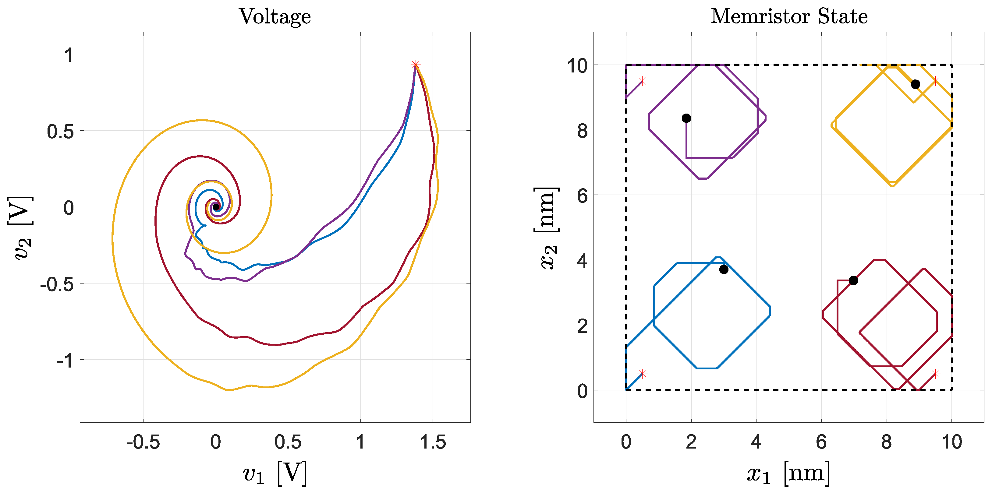
Figure 1 shows the solutions obtained starting from the initial conditions thus defined. It can be observed that, in all the simulations, the voltages converge to 0, as predicted by Theorem 1, even if the trajectories are influenced by the memristor state initial conditions and dynamics. However, note that the asymptotic values of the memristor states are different for each simulation, i.e., they depend upon the initial conditions.

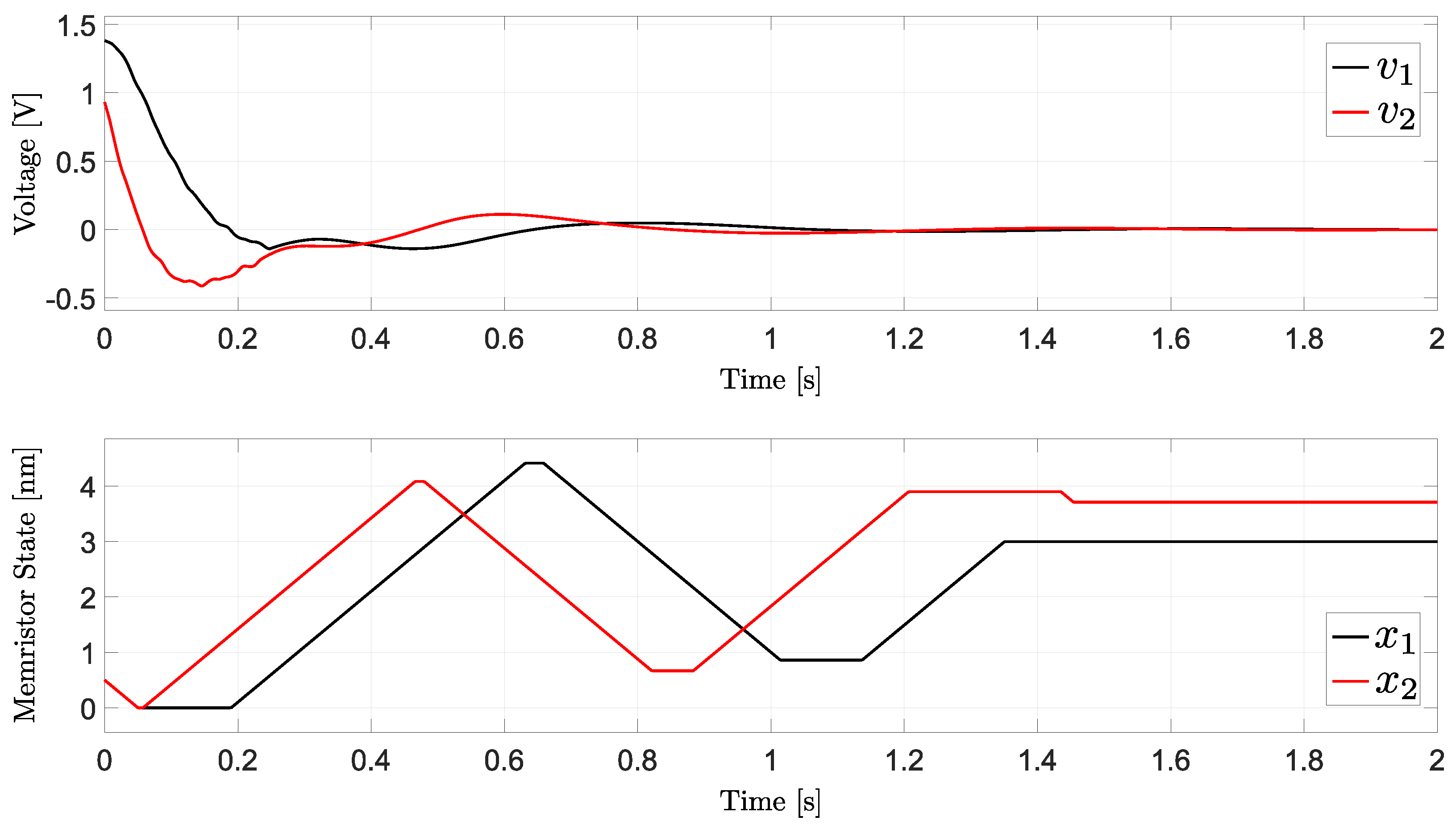
Figure 2 shows the time behavior of the specific simulation performed with initial condition $X_1\left(0\right)={\left(0.5,0.5\right)}^{\top }$ nm. From the plot, we can see that when the voltages reach the threshold $v_{on}$ ($v_{off}$), the memristor dynamics stops, i.e., the memristor states do not change anymore.

6.2. Example 2

In the second example, we set the initial conditions for the memristor states at

$$X\left(0\right)=\left(\begin{array}{c}5\\ 5\end{array}\right)\mathrm{nm}$$

(54)

and we evaluated the system dynamics starting from four different sinusoidal initial conditions for the neurons voltages, i.e.,

$$\begin{array}{c}{V}_1\left(t\right)=\left(\begin{array}{c}-2.35sin(50\pi t+0.2\pi )\\ -1.15sin(80\pi t+0.3\pi )\end{array}\right)\mathrm{V}\\ V_2\left(t\right)=\left(\begin{array}{c}-2.35sin(50\pi t+0.2\pi )\\ 1.15sin(80\pi t+0.3\pi )\end{array}\right)\mathrm{V}\\ V_3\left(t\right)=\left(\begin{array}{c}2.35sin(50\pi t+0.2\pi )\\ -1.15sin(80\pi t+0.3\pi )\end{array}\right)\mathrm{V}\\ V_4\left(t\right)=\left(\begin{array}{c}2.35sin(50\pi t+0.2\pi )\\ 1.15sin(80\pi t+0.3\pi )\end{array}\right)\mathrm{V}.\end{array}$$

(55)

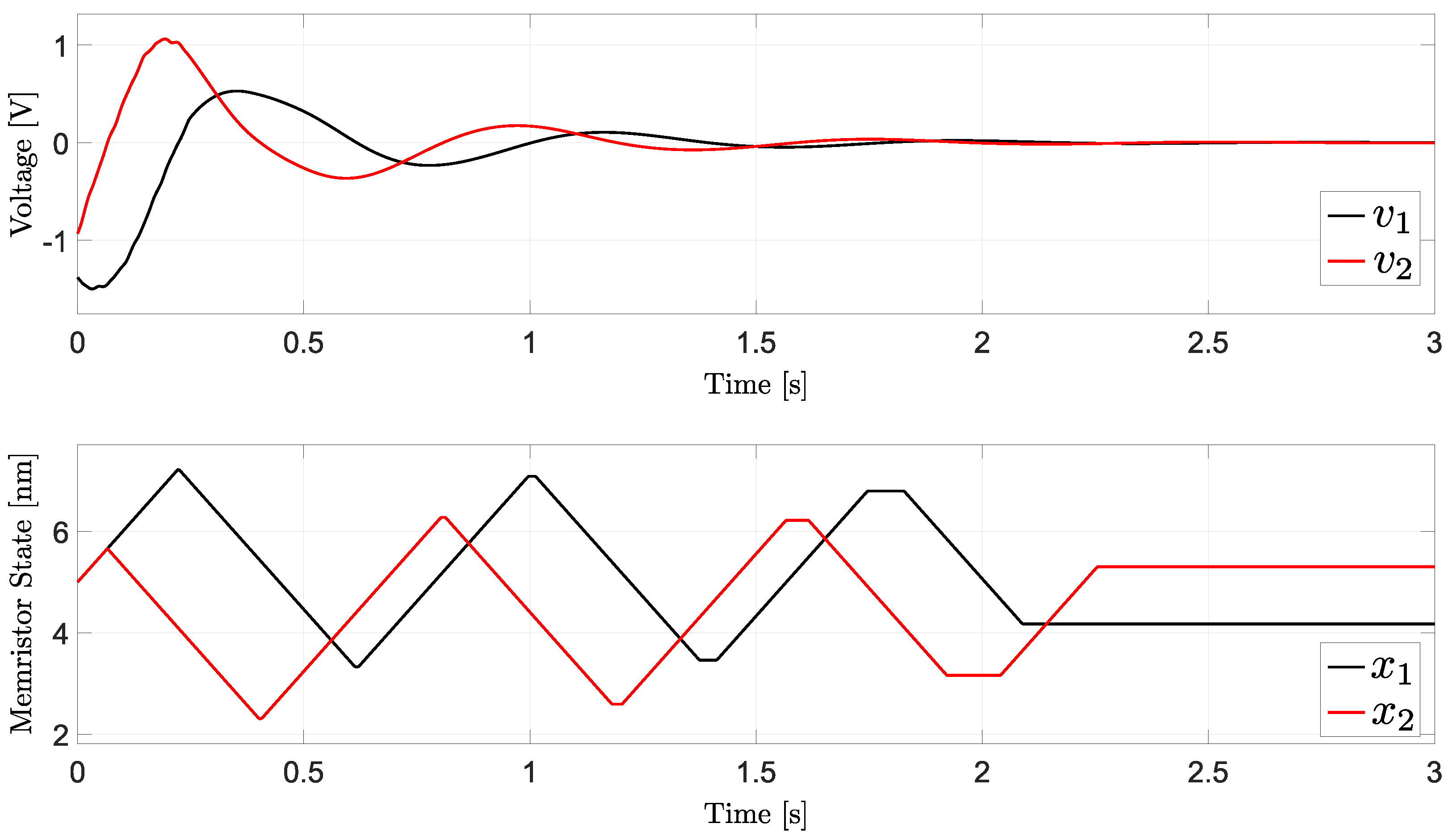
Figure 3 shows the solutions obtained starting from the initial conditions defined above. The simulations show that, regardless of the initial condition, memristor voltages always converge to 0. The different evolution in time of the neuron voltages, however, determines different dynamics of the memristor states. In fact, even if the initial memristor state is the same in each of the four analyzed cases, the subsequent dynamics are different, with the memristors that reach different asymptotic values for its states at the end of each simulation. This is better illustrated in Figure 4 for the simulation performed with initial condition $V_1\left(t\right)={\left(-2.35sin(50\pi t+0.2\pi ),-1.15sin(80\pi t+0.3\pi )\right)}^{\top }$ V.

7. Conclusions

The paper has established some fundamental results on trajectory convergence for a class of differential inclusions, which are named DVIs, modeling delayed neural networks with real generic memristors obeying the VTEAM model. The conditions for convergence hold for any constant delay and they can be applied to nonsymmetric neuron interconnection matrices. Moreover, they can be effectively checked numerically since they are expressed in the form of LMIs. Although VTEAM can be used to fit several real memristor models, it is of interest in future work to extend the obtained results to other classes of real memristors, such as those modeled by extended memristors.

References

- Waldrop, M.M. The chips are down for Moore’s law. Nat. News 2016, 530, 144. [Google Scholar] [CrossRef] [PubMed] [Green Version]
- Williams, R.S. What’s Next? [The end of Moore’s law]. Comp. Sci. Eng. 2017, 19, 7–13. [Google Scholar] [CrossRef]
- Zidan, M.A.; Strachan, J.P.; Lu, W.D. The future of electronics based on memristive systems. Nat. Electron. 2018, 1, 22. [Google Scholar] [CrossRef]
- Yang, J.J.; Williams, R.S. Memristive devices in computing system: Promises and challenges. ACM J. Emerg. Technol. Comput. Syst. 2013, 9, 11. [Google Scholar] [CrossRef]
- Li, C.; Wang, Z.; Rao, M.; Belkin, D.; Song, W.; Jiang, H.; Yan, P.; Li, Y.; Lin, P.; Hu, M.; et al. Long Short-Term Memory Networks Memristor Crossbar Arrays. Nat. Mach. Intell. 2019, 1, 49. [Google Scholar] [CrossRef]
- Ielmini, D.; Pedretti, G. Device and Circuit Architectures for In-Memory Computing. Adv. Intell. Syst. 2020, 2, 2000040. [Google Scholar] [CrossRef]
- Ielmini, D.; Wong, H.S.P. In-memory computing with resistive switching devices. Nat. Electron. 2018, 1, 333–343. [Google Scholar] [CrossRef]
- Xia, Q.; Yang, J.J. Memristive crossbar arrays for brain-inspired computing. Nat. Mater. 2019, 18, 309–323. [Google Scholar] [CrossRef]
- Chua, L.O. Memristor-The missing circuit element. IEEE Trans. Circuit Theory 1971, 18, 507–519. [Google Scholar] [CrossRef]
- Chua, L.O.; Kang, S.M. Memristive devices and systems. Proc. IEEE 1976, 64, 209–223. [Google Scholar] [CrossRef]
- Hajri, B.; Aziza, H.; Mansour, M.M.; Chehab, A. RRAM device models: A comparative analysis with experimental validation. IEEE Access 2019, 7, 168963–168980. [Google Scholar] [CrossRef]
- Chen, P.Y.; Yu, S. Compact modeling of RRAM devices and its applications in 1T1R and 1S1R array design. IEEE Trans. Electron Devices 2015, 62, 4022–4028. [Google Scholar] [CrossRef]
- Mazumder, P.; Kang, S.M.; Waser, R. Special issue on memristors: Devices, models, and applications. Proc. IEEE 2012, 100, 1911–1919. [Google Scholar] [CrossRef]
- Chua, L. Everything You Wish to Know about Memristors But Are Afraid to Ask. Radioengineering 2015, 24, 319–368. [Google Scholar] [CrossRef]
- Corinto, F.; Forti, M.; Chua, L.O. Nonlinear Circuits and Systems with Memristors; Springer: Berlin/Heidelberg, Germany, 2021. [Google Scholar]
- Kvatinsky, S.; Friedman, E.G.; Kolodny, A.; Weiser, U.C. TEAM: Threshold adaptive memristor model. IEEE Trans. Circuits Syst. I Reg. Pap. 2013, 60, 211–221. [Google Scholar] [CrossRef]
- Kvatinsky, S.; Ramadan, M.; Friedman, E.G.; Kolodny, A. VTEAM: A general model for voltage-controlled memristors. IEEE Trans. Circuits Syst. II Express Briefs 2015, 62, 786–790. [Google Scholar] [CrossRef]
- Khalid, M. Review on various memristor models, characteristics, potential applications, and future works. Trans. Electr. Electron. Mater. 2019, 20, 289–298. [Google Scholar] [CrossRef]
- Ascoli, A.; Corinto, F.; Senger, V.; Tetzlaff, R. Memristor model comparison. IEEE Circuits Syst. Mag. 2013, 13, 89–105. [Google Scholar] [CrossRef]
- Haykin, S. Neural Networks: A Comprehensive Foundation; Prentice-Hall: Hoboken, NJ, USA, 1999. [Google Scholar]
- Chua, L.O.; Yang, L. Cellular neural networks: Theory. IEEE Trans. Circuits Syst. 1988, 35, 1257–1272. [Google Scholar] [CrossRef]
- Chua, L.O.; Yang, L. Cellular neural networks: Applications. IEEE Trans. Circuits Syst. 1988, 35, 1273–1290. [Google Scholar] [CrossRef]
- Cohen, M.A.; Grossberg, S. Absolute stability of global pattern formation and parallel memory storage by competitive neural networks. IEEE Trans. Syst. Man Cybern. 1983, 13, 815–825. [Google Scholar] [CrossRef]
- Hirsch, M. Convergent activation dynamics in continuous time networks. Neural Netw. 1989, 2, 331–349. [Google Scholar] [CrossRef] [Green Version]
- Chua, L.O. Special Issue on Nonlinear Waves, Patterns and Spatio-temporal Chaos in Dynamic Arrays. IEEE Trans. Circuits Syst. I Fundam. Theory Appl. 1995, 42, 557–823. [Google Scholar]
- Michel, A.N.; Farrell, J.A.; Porod, W. Qualitative analysis of neural networks. IEEE Trans. Circuits Syst. 1989, 36, 229–243. [Google Scholar] [CrossRef]
- Di Marco, M.; Forti, M.; Grazzini, M.; Pancioni, L. Limit Set Dichotomy and Convergence of Cooperative Piecewise Linear Neural Networks. IEEE Trans. Circuits Syst. I Reg. Pap. 2011, 58, 1052–1062. [Google Scholar] [CrossRef]
- Di Marco, M.; Forti, M.; Grazzini, M.; Pancioni, L. Convergent Dynamics of Nonreciprocal Differential Variational Inequalities Modeling Neural Networks. IEEE Trans. Circuits Syst. I Reg. Pap. 2013, 60, 3227–3238. [Google Scholar] [CrossRef]
- Zhang, H.; Wang, Z.; Liu, D. A Comprehensive Review of Stability Analysis of Continuous-Time Recurrent Neural Networks. IEEE Trans. Neural Netw. Learn. Syst. 2014, 25, 1229–1262. [Google Scholar] [CrossRef]
- Di Marco, M.; Forti, M.; Pancioni, L. Complete stability of feedback CNNs with dynamic memristors and second-order cells. Int. J. Circuit Theory Appl. 2016, 44, 1959–1981. [Google Scholar] [CrossRef]
- Di Marco, M.; Forti, M.; Pancioni, L. Convergence and Multistability of Nonsymmetric Cellular Neural Networks with Memristors. IEEE Trans. Cybern. 2017, 47, 2970–2983. [Google Scholar] [CrossRef]
- Di Marco, M.; Forti, M.; Pancioni, L. Memristor standard cellular neural networks computing in the flux–charge domain. Neural Netw. 2017, 93, 152–164. [Google Scholar] [CrossRef]
- Corinto, F.; Forti, M. Memristor Circuits: Flux–Charge Analysis Method. IEEE Trans. Circuits Syst. I Reg. Pap. 2016, 63, 1997–2009. [Google Scholar] [CrossRef] [Green Version]
- Yao, W.; Wang, C.; Cao, J.; Sun, Y.; Zhou, C. Hybrid multisynchronization of coupled multistable memristive neural networks with time delays. Neurocomputing 2019, 363, 281–294. [Google Scholar] [CrossRef]
- Nie, X.; Zheng, W.X.; Cao, J. Multistability of memristive Cohen-Grossberg neural networks with non-monotonic piecewise linear activation functions and time-varying delays. Neural Netw. 2015, 71, 27–36. [Google Scholar] [CrossRef] [PubMed]
- Pershin, Y.V.; Di Ventra, M. On the validity of memristor modeling in the neural network literature. Neural Netw. 2020, 121, 52–56. [Google Scholar] [CrossRef]
- Chua, L.O.; Roska, T. Cellular Neural Networks and Visual Computing: Foundation and Applications; Cambridge University Press: Cambridge, UK, 2005. [Google Scholar]
- Yin, W.; Yang, W.; Liu, H. A neural network scheme for recovering scattering obstacles with limited phaseless far-field data. J. Comput. Phys. 2020, 417, 109594. [Google Scholar] [CrossRef]
- Aubin, J.P.; Cellina, A. Differential Inclusions. Set-Valued Maps and Viability Theory; Springer: Berlin, Germany, 1984. [Google Scholar]
- Boyd, S.P.; El Ghaoui, L.; Feron, E.; Balakrishnan, V. Linear Matrix Inequalities in System and Control Theory; SIAM: Philadelphia, PA, USA, 1994; Volume 15. [Google Scholar]
- Aubin, J.P.; Frankowska, H. Set-Valued Analysis; Birkauser: Boston, MA, USA, 1990. [Google Scholar]
- Di Marco, M.; Forti, M.; Grazzini, M.; Pancioni, L. On global exponential stability of standard and full-range CNNs. Int. J. Circuit Theory Appl. 2008, 36, 653–680. [Google Scholar] [CrossRef]
- Hopfield, J. Neural Networks and Physical Systems with Emergent Collective Computational Abilities. Proc. Natl. Acad. Sci. USA 1982, 79, 2554–2558. [Google Scholar] [CrossRef] [Green Version]
- Sanchez, E.N.; Perez, J.P. Input-to-state stability (ISS) analysis for dynamic neural networks. IEEE Trans. Circuits Syst. I Fundam. Theory Appl. 1999, 46, 1395–1398. [Google Scholar] [CrossRef]
Figure 1.
Simulations of the memristor neural network considered in Example 1. Each color represents a different solution, obtained for a specific memristor initial condition. The initial conditions are labeled by the red markers. The final memristor states are labeled by the black dots. The black dashed box in the right plot is the hypercube bounding the memristor states.
Figure 2.
Time domain behavior for the solution in Example 1 having initial condition nm.
Figure 3.
Simulations of the memristor neural network considered in Example 2. Each color represents a different solution, obtained for a specific memristor initial condition. The initial conditions are labeled by the red markers. The final memristor states are labeled by the black dots. The black dashed box in the right plot is the hypercube bounding the memristor states.
Figure 4.
Time domain behavior for the state solution in Example 2 with V.
Publisher’s Note: MDPI stays neutral with regard to jurisdictional claims in published maps and institutional affiliations. |
© 2022 by the authors. Licensee MDPI, Basel, Switzerland. This article is an open access article distributed under the terms and conditions of the Creative Commons Attribution (CC BY) license (https://creativecommons.org/licenses/by/4.0/).
Share and Cite
MDPI and ACS Style
Di Marco, M.; Forti, M.; Moretti, R.; Pancioni, L.; Innocenti, G.; Tesi, A. Convergence of a Class of Delayed Neural Networks with Real Memristor Devices. Mathematics 2022, 10, 2439. https://doi.org/10.3390/math10142439
AMA Style
Di Marco M, Forti M, Moretti R, Pancioni L, Innocenti G, Tesi A. Convergence of a Class of Delayed Neural Networks with Real Memristor Devices. Mathematics. 2022; 10(14):2439. https://doi.org/10.3390/math10142439
Chicago/Turabian StyleDi Marco, Mauro, Mauro Forti, Riccardo Moretti, Luca Pancioni, Giacomo Innocenti, and Alberto Tesi. 2022. "Convergence of a Class of Delayed Neural Networks with Real Memristor Devices" Mathematics 10, no. 14: 2439. https://doi.org/10.3390/math10142439
Note that from the first issue of 2016, this journal uses article numbers instead of page numbers. See further details here.