An Automata-Based Cardiac Electrophysiology Simulator to Assess Arrhythmia Inducibility

Abstract

Personalized cardiac electrophysiology simulations have demonstrated great potential to study cardiac arrhythmias and help in therapy planning of radio-frequency ablation. Its application to analyze vulnerability to ventricular tachycardia and sudden cardiac death in infarcted patients has been recently explored. However, the detailed multi-scale biophysical simulations used in these studies are very demanding in terms of memory and computational resources, which prevents their clinical translation. In this work, we present a fast phenomenological system based on cellular automata (CA) to simulate personalized cardiac electrophysiology. The system is trained on biophysical simulations to reproduce cellular and tissue dynamics in healthy and pathological conditions, including action potential restitution, conduction velocity restitution and cell safety factor. We show that a full ventricular simulation can be performed in the order of seconds, emulate the results of a biophysical simulation and reproduce a patient’s ventricular tachycardia in a model that includes a heterogeneous scar region. The system could be used to study the risk of arrhythmia in infarcted patients for a large number of scenarios.

1. Introduction

Over the last few decades, there have been published an increasing number of mathematical models that describe, with a great level of detail, cardiac cell function [1,2]. These mathematical cell models are defined by a set of differential equations that take into account the cell ion dynamics and ion concentrations in the intracellular and extracellular space, among others. As a result, the models can be used to study cell electrical dynamics, the response to different drugs or the changes under pathological conditions such as ischemia.

Cellular models can be combined as building blocks to perform tissue-level or organ-level computer simulations, i.e., simulations of the whole atria, or the full four chambers of the heart. These multi-scale reaction–diffusion models are commonly based on differential equations that allow us to simulate the electrical diffusion on tissue, and are coupled to cellular ionic models that provide the electrical current (reaction term) at the cell level [3]. Two widely used mathematical approaches to simulate electrical propagation on tissue are the so-called bidomain and monodomain models [4].

In order to study cardiac diseases, mathematical models of cell and tissue activity are usually combined with detailed geometrical descriptions of the domain of interest, i.e., a three-dimensional representation of the heart [5]. There are several methodologies to obtain these geometrical models, from synthetic mathematical representations (3D ellipsoids) to faithful anatomical models obtained by the segmentation of myocardial tissue from medical images such as magnetic resonance imaging. Anatomical domains should be discretized by building a volumetric mesh, i.e., a representation where finite element methods (FEM) or alternative numerical schemes can be used to solve cardiac electrophysiology equations. However, the spatial and temporal discretization required by these methods is very high, in the order of 250–300 $\mathsf{\mu }$m and 10–20 $\mathsf{\mu }$s, which makes the solution of a single heartbeat very challenging. Although there exist several software packages that implement part of these methods (Elvira [6], Chaste [7], or openCARP [8]), they still rely on high performance computing and require specific expertise to set up biophysical simulations and build 3D meshes that meet all mathematical requirements.

Once all the anatomical and functional information is combined, the model can be used to study the mechanisms of arrhythmia in patients, stratify patients, or plan non-invasively for interventions such as radio-frequency ablation (RFA) [2,9,10,11] or cardiac resynchronization therapy. Although recent studies have demonstrated the potential of in silico approaches, there is still debate about the necessary level of detail on the mode to be able to obtain meaningful and accurate clinical results [12,13,14]. For the particular application of simulating and predicting the risk of sudden cardiac death of a subject who has suffered a myocardial infarction, detailed biophysical models have been proposed because they can specifically model the heterogeneous properties of ischemic tissue [5,10,15,16]. Biophysical and phenomenological models have been successfully used to predict the slow conduction channel that sustains a patient’s tachycardia, and even induce the same arrhythmic episodes in silico by a virtual pace mapping protocol. In general, these studies make use of models with a high computational cost (hours or days to simulate a protocol of few seconds), and require specific expertise to construct the computational finite element model and run the biophysical solver. Computational models with reduced complexity that are able to produce accurate results for the target clinical application are necessary to permit the clinical translation and promote uptake [13,17,18,19].

In this work, we first review the current mathematical models used to simulate cardiac electrophysiology with an emphasis on ventricular arrhythmia, and propose as an alternative method the use of advanced physiological cellular automaton (CA). The method proposed includes a specific encoding of the dynamic electrical properties of myocardial cell and tissue for both healthy and pathological (post-infarct) conditions, which allows the efficient simulation of cardiac electrophysiology in patients who have a myocardial scar. First, we inform the CA by means of controlled biophysical simulations, and test its response on a simplified geometrical tissue model. Next, we make use of the CA in a personalized ventricular model, including a heterogeneous scar, where we reproduce the results of a complex biophysical model, with very low computational cost, resulting in a speed-up of 311×.

2. Material and Methods

2.1. Biophysical Modeling of Cardiac Cells

Most biophysical cardiac action potential (AP) models (see Figure 1a, curve on purple background) are based on the original formulation by Hodgkin and Huxley [20], which considers the cell membrane as a set of gated ion channels. These gates allow or block the different ions going through the cell membrane depending on factors such as the membrane potential or the concentration of certain ions in the different domains. Therefore, the cell membrane may be modeled with an equivalent electric circuit, which is a set of resistances connected in parallel to a capacitor and batteries, representing the different pumps and ionic currents. In this circuit, $C_m$ is the capacity of the cell membrane, and $I_j$ will represent the electrical currents across the membrane (sodium $N{a}^{+}$, potassium $K^{+}$, calcium $C{a}^{2+}$). The membrane potential can then be calculated as

$$\frac{d{V}_m}{dt}=-\frac{1}{C_m}·I_{ion},$$

(1)

$$I_{ion}=I_{K1}+I_{Na}+I_{to}+I_{Ks}+I_{Kr}+I_{CaL}+I_{NaCa}+I_{NaK}+I_{pK}+I_{pCa}+I_{bNa}+I_{bCa},$$

(2)

$$I_j=g_j·(V_m-E_j),$$

(3)

where $E_j$ is the channel equilibrium potential associated with ion j, and $g_j$ is the time-dependent value of conductance. Note that, in addition to the currents associated with each ion, the membrane also includes pumps and exchangers that alter the ionic concentrations inside and outside the cell. The time-dependent conductance of each ion channel j is modulated by the channel density in the membrane, the unitary conductance of the particular ion j, and the fraction of open channels at a given time point, which in turn depends on the voltage and the concentration of ion j in the intracellular and extracellular domains.

From the first model [20] and the development of patch clamp techniques that allow us to experimentally measure currents that cross the membrane, a number of mathematical models have been defined. Among the human cell ionic models, we can highlight the models proposed by ten Tusscher et al. [21], Grandi et al. [22], O’Hara et al. [23], and Tomek et al. [24].

In this study, we base our biophysical simulations on the ten Tusscher et al. model for ventricular myocytes [21], which has been extensively validated over the last few years and applied to model cardiac arrhythmia [5]. The model considers transmural heterogeneity by modeling differently subendocardial, midmyocardial, and epicardial cells [25]. Another important characteristic that we seek in the model is that it can reproduce the measured action potential duration restitution (APDR) [26,27,28] (see Figure 1a) and conduction velocity restitution (CVR) [29,30] (see Figure 1b) properties of the human myocardium, which are very important for the occurrence and stability of reentrant arrhythmias.

To model the scar region, and in particular its border zone (BZ), we make use of a modified version of the ten Tusscher model [31], aiming to reproduce the altered electrical behavior (electrical remodeling) of the surviving myocytes. Therefore, in the scar BZ, the following parameters were adjusted as in [5]: (i) reduction of the conductance of peak sodium current ($I_{Na}$) to 38% of its normal value ($g_{Na}\times 0.38$); (ii) reduction of L-type calcium current ($I_{CaL}$) to 31% ($0.31\times g_{Na}$); and (iii) reduction of rapid and slow delayed rectifying potassium currents ($I_{Kr}$ and $I_{Ks}$) to 30% and 20% of their values ($0.3\times g_{Kr}$ and $0.2\times g_{Ks}$), respectively. The main expected effects of the applied changes are the prolongation of the action potential duration (APD) and a decrease in the AP upstroke velocity and maximum amplitude.

2.2. Biophysical Modeling of Cardiac Tissue

A common approach used to mathematically model cardiac tissue is based on a reaction–diffusion equation known as the bidomain model. The bidomain model allows us to consider the coupling of myocytes and the diffusion of current through the myocardial tissue [32]. In this mathematical formulation, the cell membrane acts as a capacitor, separating two domains (intracellular and extracellular), and compensates for the load on both sides. Since the current flow at each point must be a balance between the incoming and the outgoing current, the following expressions may be inferred:

$$-\nabla ·J_i=\frac{\partial q_i}{\partial t}+\chi I_{ion}$$

(4)

$$-\nabla ·J_e=\frac{\partial q_e}{\partial t}+\chi I_{ion}$$

(5)

$$\nabla ·J_i+\nabla ·J_e=0$$

(6)

where $J_i$ and $J_e$ are the ionic current densities, and $q_i$ and $q_e$ are the charges in the intra- and extracellular domains, respectively. $I_{ion}$ is the current across the membrane and $\chi$ is the area of the membrane per unit volume. Note that $I_{ion}$ is obtained from the underlying cellular model connected to the bidomain as given by (2), and represents the reaction term.

The membrane potential $V_m$ depends on both the membrane capacity and the potential difference between the intracellular and extracellular domains according to the following equation:

$$V_m=\frac{Q}{C_m}$$

(7)

with $C_m$ the membrane capacitance, and q the charge. Combining all previous equations, we can obtain the elliptic–parabolic formulation of the bidomain model in the heart domain (${\Omega }_H$) as

$$\nabla ·({\mathbf{D}}_i\nabla V_m)+\nabla ·({\mathbf{D}}_i\nabla V_e)=C_m·\frac{\partial V_m}{\partial t}+I_{ion},$$

(8)

$$\nabla ·({\mathbf{D}}_i\nabla V_m)+\nabla ·(({\mathbf{D}}_i+{\mathbf{D}}_e)\nabla V_e)=0,$$

(9)

where D is the diffusion tensor in each domain, and $V_m$ the membrane potential. A set of boundary conditions have to be defined to solve the bidomain equations. First, we assume that the heart is surrounded by a non-conductive medium, and therefore the normal component of the intracellular and extracellular currents must be zero along the boundary, $\partial {\Omega }_H$, and then,

$$n·({\mathbf{D}}_i\nabla V_m)+{\mathbf{D}}_i\nabla V_e)=0,$$

(10)

$$n·\nabla ({\mathbf{D}}_e\nabla V_e)=0.$$

(11)

It is noteworthy to comment that the solution of the bidomain equations is very demanding computationally, and therefore a simplification known as the monodomain equation is commonly used. Monodomain assumes that variations in the extracellular potential are very small compared to those in the intracellular domain, and that there exist equal anisotropy ratios in the conductivity tensors, $D_e=\lambda ·D_i$. These assumptions give rise to

$$\nabla ·(\mathbf{D}\nabla V_m)=C_m·\frac{\partial V_m}{\partial t}+I_{ion},$$

(12)

$$n·\nabla (\mathbf{D}\nabla V_m)=0.$$

(13)

In this study, we will perform all the biophysical simulations using the monodomain formulation, which will be considered the ground-truth data, since we are only interested in the evolution of the membrane potential in the heart domain. The simulations were carried out with the cardiac biophysical solver ELVIRA [6], on a machine comprising 128 GB of RAM and 64-bit AMD processors with a total of 64 cores at 2.3 GHz (4× AMD Opteron 6376 processor). Regarding our particular simulations, we applied the conjugate gradient method with an integration time step (dt) of 0.02 ms to compute the numerical solution. Our spatial discretization is determined by the spatial resolution of the FEM volume mesh that defines the geometry of the problem. Thus, in our biophysical simulations, spatial discretization was of 0.3 mm, both for organ simulations with the 3D ventricular model and for test simulations with the 3D slab model. Furthermore, we used implicit integration for the parabolic partial differential equation (PDE) of the monodomain model (tissue level) and explicit integration with adaptive time stepping for systems of ordinary differential equations (ODE) associated with ionic models used at cellular level.

2.3. Cellular Automaton Electrophysiology Model

We made use of an event-based asynchronous cellular automaton to model cardiac electrophysiology spatially extended. Although it is common to use cell to denote each computation unit of CA, in order to prevent confusion with cardiac cardiomyocytes, we will use node to refer to each element of the automaton. Therefore, each node represents a portion of tissue, and not a single cardiac cell, following a continuous representation. Cardiac models based on traditional CA are qualitative, and do not follow the Hodgkin–Huxley formulation to describe channel electrical activity at cell level.

Cardiac tissue is discretized in a set of nodes and elements, where each node can be in two main states: active (depolarized) or inactive (repolarized). When an inactive node is excited by its neighbors or an external stimulus, it activates; during the activation phase, it can excite other surrounding nodes; it stays active over its APD and cannot be activated again until this time expires. When AP reaches the resting state (APD), the node is repolarized and returns to the inactive state. The lapse of time between the inactivation and a new successful activation is called the diastolic interval (DI) (see Figure 1a, curve on green background). We have to take into account that, when a node activates, the excitation to the neighbors does not happen instantaneously; it takes a positive finite time that depends on the distance between the active and the inactive nodes and the local conduction velocity (CV).

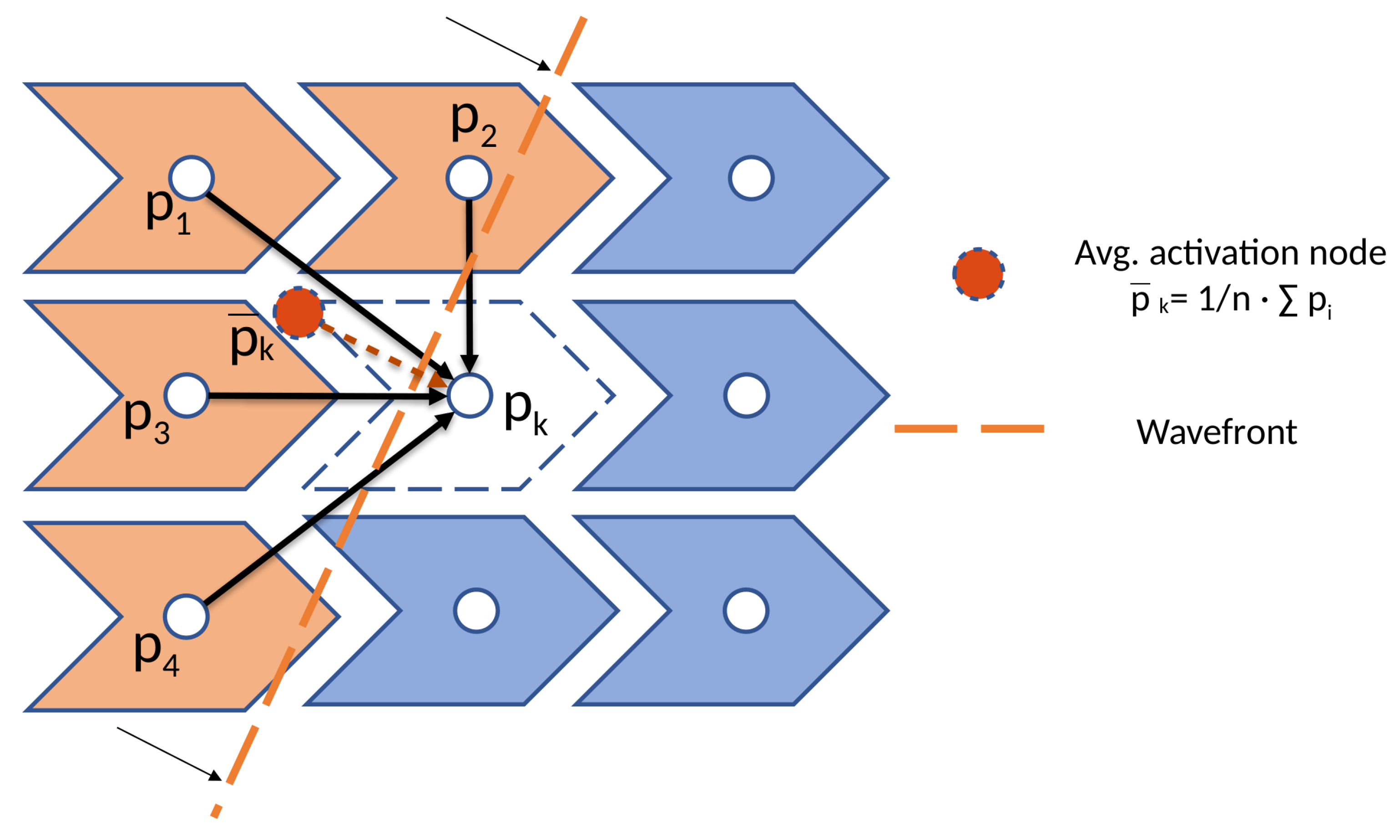
2.3.1. Cell Activation Model

Each node has two possible states: ${\sigma }_0$ representing the inactive state and ${\sigma }_1$ representing an active node. In addition, a node has an APD and a DI value assigned. These values are not fixed, but are computed according to the ten Tusscher cell model [21] by means of the restitution curves, which relate the next APD to the previous DI (see Figure 1). The computation of such curves is discussed in Section 2.5.

Since there are only two states, only two possible transitions can happen: activation (${\sigma }_0\to {\sigma }_1$) and inactivation (${\sigma }_1\to {\sigma }_0$). The transitions between states for a node are event-based. This means that whenever a transition is expected, an event is generated including the transition time and the transition type.

The activation of a node (transition from ${\sigma }_0$ to ${\sigma }_1$) happens as a result of the action potential generated by nearby active nodes. The activation reaches a certain location, advancing as a wavefront that travels at the CV defined by the tissue and the nodes that form it. For a given inactive node that is close to other recently activated nodes, we need to compute its activation time. In order to model activation, we follow a scheme similar to the Fast Marching algorithm [33]. We assume that the wavefront can be approximated locally as a plane in the 3D tissue (a straight line in a 2D domain) that travels in the direction of its normal. For each inactive node, k, the average location of its n active neighbors is computed, ${\overline{p}}_k=\frac{1}{n}{\sum }_i{p}_i$, together with the average activation time, ${\overline{t}}_k=\frac{1}{n}{\sum }_i{t}_i^a$. Then, the activation time is computed as $t_k^a={\overline{t}}_k+d({\overline{p}}_k,p_k)/v_k$, with $d({\overline{p}}_k,p_k)$ the distance from ${\overline{p}}_k$ to node k. Figure 2 shows a schematic of this approach; node k is activated by four of its neighbors, $p_1,p_2,p_3$ and $p_4$.

When a node i activates, it also generates an inactivation event for itself at time $t_i^d=t_i^a+AP{D}_i$, being $AP{D}_i$ the APD of node i. In order to add the dynamic myocytes’ response into the model, we make use of the DI, and obtain the APD and CV after each activation event by means of the restitution curves (see Figure 1). We also include some additional terms, such as APD memory. As described in [34], the ten Tusscher model exhibits a substantial degree of short-term cardiac memory, which requires a time of accommodation when the cycle length varies. The S1–S2 stimulation protocol was used to account for all possible scenarios of activation patterns, including the ones used in the EP room to trigger arrhythmias. In the absence of short-term memory, S1–S2 restitution curves with different S1 would result in the same AP. However, these models possess a memory of pacing history and therefore are not only dependent on the previous DI, but also the previous S1 and APD. Therefore, we consider this memory by averaging the next APD (dependent on DI) with the previous APD (dependent on S1). In particular, we weighted the previous APD, $10\%$, and next APD, ($90\%$ of the values), which ensures smooth temporal transitions in APD when large changes in cycle length pacing (e.g., S1–S2 protocols) are applied. In addition, the model takes into account the electrotonic coupling effects by smoothing the APD properties of each node with its neighbor nodes, which are key in regions where there is the presence of adjacent heterogeneous tissue (pathological and healthy nodes). To do so, we performed a weighted average of the APD for a given node, with the surrounding (directly connected) activated nodes, to avoid large non-physiological gradients. The smoothing factor is an input parameter.

Axisymmetric fiber orientation is included by adding a ratio of longitudinal versus traversal CV in the model to account for differences in propagation along the fiber and across fiber directions of cardiac tissue. Due to the lack of clinical data, transmural conduction was considered the same as the transversal fiber orientation conductivity.

2.3.2. Tissue Modeling

The nodes of the automaton are distributed along the cardiac tissue, forming three-dimensional elements. The initial activation, e.g., through the defined pacing protocol, introduces the activation event for the stimulated nodes. During the simulation, the events are processed one at a time. The first event in the queue is taken, and the corresponding node is activated or in resting state. If the event corresponds to an activation transition, then the activation events for the node’s neighbors are created and inserted in the queue. The simulation time advances with the time of the last processed event. As a consequence, the simulator does not have a time step as such.

We have to take into account that for a given inactive node k, we do not know beforehand which neighbors are going to activate before it does, and become activating nodes, contributing to the average activating location ${\overline{p}}_k$. Thus, for each neighbor i that activates before node k does, the average location ${\overline{p}}_k=\frac{1}{n}\sum p_i$ is updated and the corresponding event is generated. As a consequence, during the propagation process, several activation events are generated for most inactive nodes. This is not an issue from the simulation point of view, since the first event that is taken from the queue is processed, activating node k, and any subsequent event is ignored, since the transition cannot take place.

Algorithm 1 describes the activation process. Note that there is no time step in the simulation process, and the priority queue is modified while it is processed. Note that it is not possible to generate an event after the time it should have been triggered.

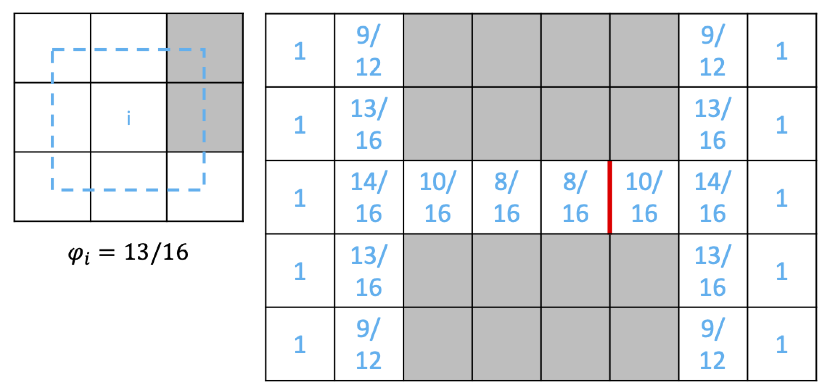
2.3.3. Safety Factor

The cardiac safety factor (SF) is a measure of the robustness of propagation in cardiac tissue, which relates the current received by a cell with respect to the amount required to trigger its depolarization or activation. Several formulations have been proposed to quantify the SF [35,36]. In general, when SF < 1, electrical propagation from cell to cell fails (conduction block), which is one of the most common conditions to trigger and perpetuate an arrhythmia. This is especially important when there are anatomical barriers or thin surviving tissue channels, as happens in the case of slow conduction channels (SCCs) that form through the infarcted tissue. Therefore, we have developed a geometric-based approach that precomputes the SF in the simulation domain as a function of the ratio between healthy and pathological tissue.

Algorithm 1 Activation propagation method. The reader can refer to the text for details on the notation.

1: Events ← PriorityQueue()   2: Events.insert($[{\mathbf{x}}_0,t_0,act]$)                             ▷ Initial activation   3: while not Events.empty() do   4:       $[\mathbf{x},t,type]\leftarrow$ Events.pop()   5:       if type == deact then                                  ▷ Deactivation event   6:          Deactivate($\mathbf{x}$)   7:       else if type == act then                                    ▷ Activation event   8:          if IsActive($\mathbf{x}$) then                                  ▷ If $\mathbf{x}$ is active, event ignored   9:                continue 10:          else 11:                Activate($\mathbf{x}$) 12:                APD ← ComputeAPD($\mathbf{x}$, t) 13:                Events.insert($[\mathbf{x},t+APD,deact]$ 14:                for all $\mathbf{v}\in$ neighbors($\mathbf{x}$) do 15:                 if SafetyFactor($\mathbf{x}$) < SafetyFactor($\mathbf{v}$) then                ▷ Safety Factor Check 16:                       continue 17:                 end if 18:                 Update ${\overline{p}}_{\mathbf{v}}$ 19:                 Update ${\overline{t}}_{\mathbf{v}}$ 20:                 $v_{\mathbf{v}}\leftarrow$ ComputeVel() 21:                 $t_{\mathbf{v}}^a\leftarrow {\overline{t}}_{\mathbf{v}}+d({\overline{p}}_k,p_k)/v_{\mathbf{v}}$ 22:                 Events.insert($[\mathbf{v},t_{\mathbf{v}}^a,act]$) 23:                end for 24:          end if 25:       end if 26: end while

In our discretization of the tissue, we compute, for every node, the volume comprised inside the convex hull of its neighbor nodes. Then, we compute the safety factor value as the ratio between the area occupied by healthy and pathological tissue in this volume. Note that since we cannot model the current exchanged between cells, we cannot calculate the minimum current load required to activate a neighboring cell, and therefore we base our SF in the anatomical configuration of tissue. Figure 3 (left) shows an example for a planar case and a regular grid. The area inside the dashed line is the reference area for the node in the center of the grid, and its SF is the ratio between the healthy (white) area and the pathological (gray) area. During the simulation, we compare the computed SF value of the cells involved in the electrical propagation process; if an active node with SF value $s{f}_a$ tries to trigger a node with SF value $s{f}_i>s{f}_a$, then this activation is blocked. Figure 3 (right) shows an example where an SCC exists inside an infarcted region (gray cells). Propagation only occurs from cells with a higher to a lower ratio, and therefore, in the transition from cell with SF = 8/16 to SF = 10/16, there is a conduction block. The region that influences a node’s safety factor can be modified by extending the size of the neighborhood used to compute it. By defining the neighborhood as the nodes that are within a certain Euclidean distance, its definition can be made independent of the mesh resolution.

2.4. Geometry of the 3D Simulation Domains

To validate the CA and the propagation on volumetric meshes, we built a set of simplified 3D slabs of tissue with regular hexahedral elements of side length 0.3 mm (element edge), and dimensions of 50 × 50 mm in the xy-plane and variable thickness [0.3 mm, 0.9 mm] in the z-axis. The different meshes were used to perform biophysical simulations and obtain the dynamic parameters of the model that were subsequently plugged into the CA model. Fiber orientation was considered, being aligned with the y-axis. Next, we analyzed the CA model in a previous patient-specific human heart anatomy segmented from an MRI scan [5]. It corresponded to a subject with a large chronic myocardial infarction that had developed a monomorphic VT. The biventricular three-dimensional anatomical model was segmented from a de-MRI scan, and meshed with hexahedral elements with an average length of 0.4 mm. Myocardial fiber orientation was included by the Streeter model, and scar segmentation (and its respective core zone and border zone, CZ and BZ, respectively), was performed as a function of the MRI gray intensity level (BZ gray-level intensity between mean + 2 × SD). From the anatomical model, we only carried out simulations on the left ventricle (2.8 million nodes).

In this study, for the CA simulations, we made use of rectangular slabs of tissue and a left ventricle geometry obtained from a de-MRI scan, with a regular hexahedral distribution. In both cases, the distribution of nodes would be a regular grid. The neighborhood of each node was formed by all adjacent nodes including diagonals (the extension to 3D of the Moore’s neighborhood), making a total of 26 neighbors for each node.

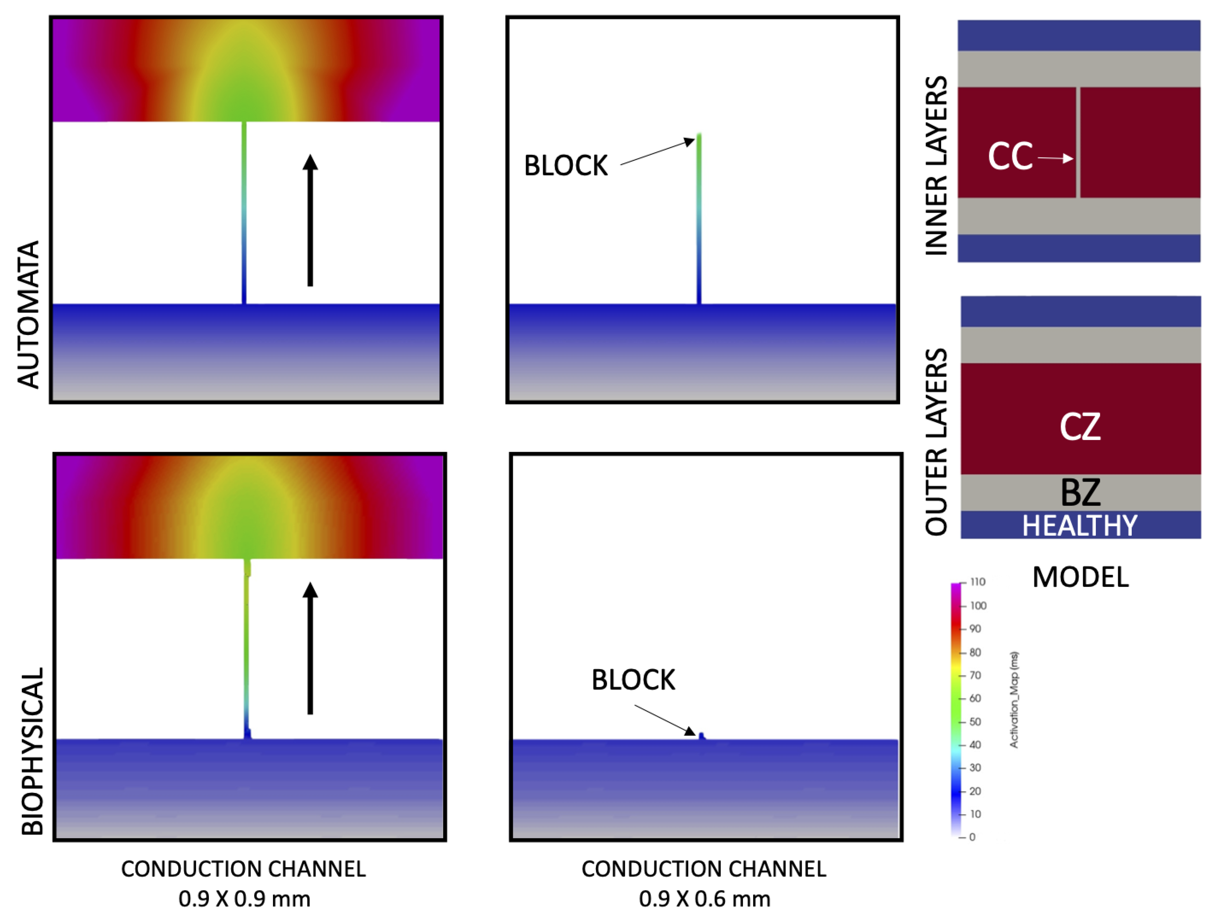
2.5. Biophysical Simulations in a Slab of Tissue

We carried out biophysical simulations in the simplified 3D slab of tissue ($50\times 50\times 0.3$ mm), combining the monodomain formulation and the ten Tusscher model including the six cell types considered (endo-, myd-, epicardium; in healthy and pathological conditions).

First of all, to obtain APDR and CVR in the 3D model, we stimulated one of the slab faces with a square pulse for 2 ms to obtain a flat propagation in the y-axis direction, as can be observed in Figure 4. To obtain the APD and CV for different DI, we performed a S1–S2 pacing protocol with a proportion of 9 S1 before an S2 to stabilize the model. The values for S1 ranged from 500 to 1000 ms in steps of 100 ms, and from 500 to 300 in steps of 20 ms to obtain better resolution in the regions with greater derivative. On the other hand, given an S1, the values of S2 ranged from S1-20 to 250 ms in order to obtain a dense enough sampling. Note that after the first S1–S2, we started from the previous state so that the APD could converge faster to a steady state, avoiding the effects of APD memory.

We used four probes separated by 9.9 mm descending the y-axis in the center of the slab, where we recorded the AP of each probe every $20\mathsf{\mu }$s during the simulations. We used the last two stimuli of each S1–S2 batch, and computed the APD${}_{90}$, i.e., the time between the maximum derivative (at the beginning of the upstroke) and the $90\%$ of repolarization. Then, we computed the DI between them as the time at the end of the APD${}_{90}$ of the first stimulus and the point with maximum derivative on the second. Finally, CV was measured as the space separating two nodes divided by the difference in the time of their maximum derivatives. All the experimental measurements have been fitted to the analytical expression

$$f\left(x\right)=a(1-bexp(-x/c\left)\right),$$

(14)

in order to obtain smooth functions allowing us both interpolation and extrapolation of values [28].

3. Results

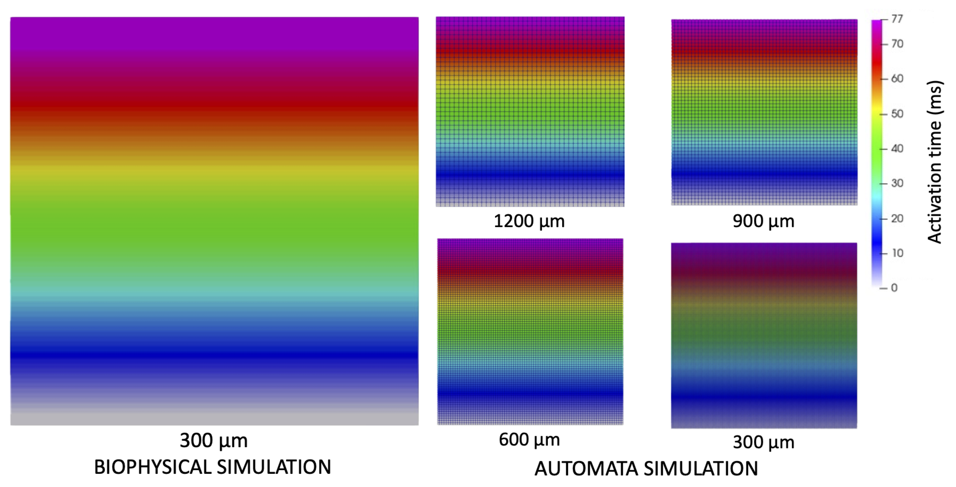
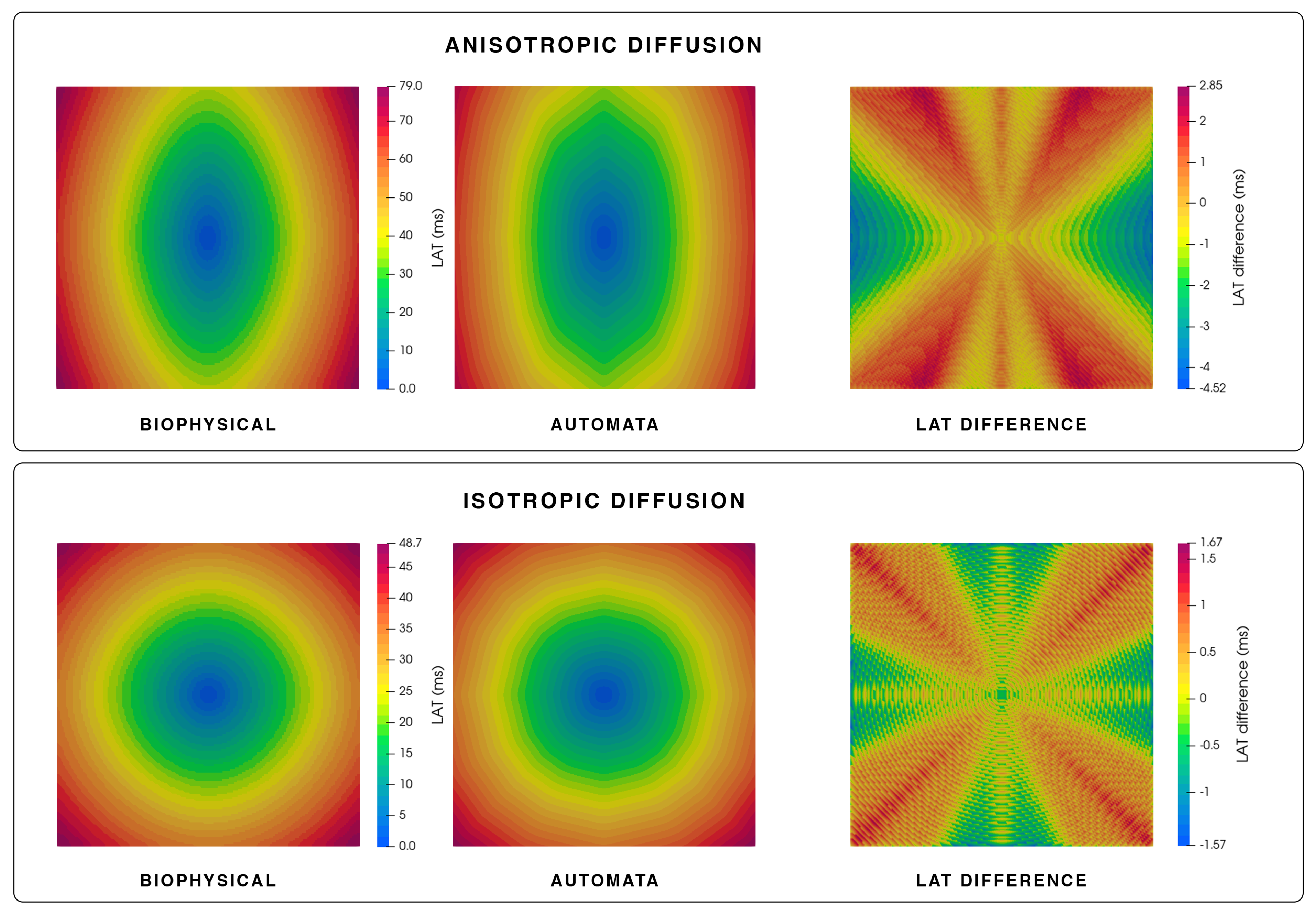
3.1. Simulation of Electrical Propagation

In order to validate the electrical propagation on the CA model adjusted to the simulated ten Tusscher model data, we performed simulations on the simple slab of tissue. Simulations using the biophysical models were run on a fine mesh ($300\mathsf{\mu }$m edge length hexahedra) to avoid artifacts on the resolution of Equation (12), which are usually observed due to the fast upstroke of the AP in the propagation wavefront. For the CA, where these restrictions do not apply, we solved the propagation using meshes with different resolutions ($300\mathsf{\mu }$m to $1200\mathsf{\mu }$m) to test the mesh independence.

Figure 4 shows the meshes color-coded with the local activation time of each node for all the scenarios simulated. In all cases, the tissue was completely activated in 77 ms, starting from the inferior side of the slab, and propagating in the y-axis, coinciding with the tissue fiber orientation defined. As can be observed, for all resolutions using the CA model, the results matched exactly the biophysical simulation. Figure 5 shows the local activation time maps produced by a single stimulus in the center of the model, where it can be appreciated the curvature of the propagation wavefront (first and second columns), and the difference between the biophysical and CA models (third column). For both isotropic and anisotropic diffusion, the main differences are observed in the diagonal, and they accumulate as a function of the distance. This means that the wavefront curvature in the CA model does not evolve properly and loses circularity, which translates into a propagation delay of 2.8 ms at a distance of 3.5 cm from the source.

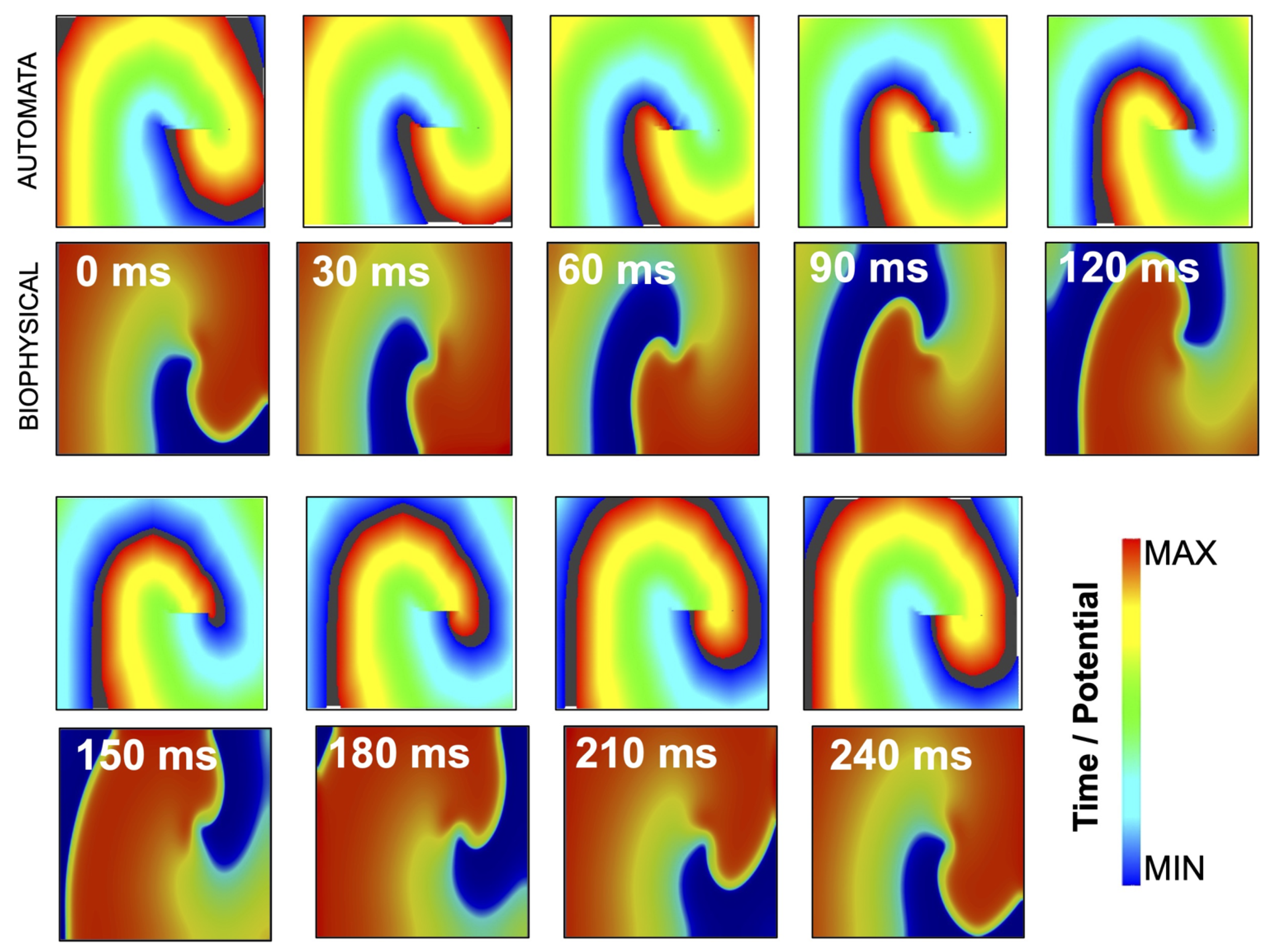
3.2. Simulation of Rotor Dynamics

To test complex scenarios in which the model has to consider local changes in CV and APD due to short and heterogeneous DIs, which are not homogeneously distributed, we simulated spiral wave scenarios, i.e., the so-called rotors. As done in experimental scenarios, we study, in a healthy slab of tissue, the feasibility to trigger spiral wave activity by means of an S1–S2 cross-field protocol. Figure 6 shows the patterns obtained at different time instants after applying five flat S1 stimuli (basic cycle length (BCL) of 500 ms) on the lower side of the slab model, followed by a single S2 stimulus (BCL of 400 ms) coupled to the tail of the action potential. A spiral wave formed right after the S2 stimulus, but the rotor tip and the CV needed at least 3000 ms to stabilize. Figure 6 compares, every 30 ms, the dynamics of the spiral wave for the CA and the biophysical model. In both cases, the spiral wave rotation period was 250 ms, and there was a localized meandering of the tip. Colors in the CA simulations represent the time (in ms) for a given cell to arrive to the resting or inactive state, which decreases linearly since the cell is activated. On the other hand, color from biophysical simulations corresponds to potential (in mV), which decreases following the shape of the AP. Note that, since the CA cells are either in active or in resting state, with no intermediate states that the biophysical simulation can reproduce, the depolarization wavefront around the rotor tip shows the propagation block as a straight line in the active vs. resting area edge. Although the CA simulation does not account for ionic source–sink effects related to wavefront curvature, the biophysical simulation and the CA simulation are comparable.

To obtain comparative results between CA and biophysical simulations after several activations or heartbeats, dynamic parameters that depend on DI (CVR and APDR) must advance in parallel. The introduction of APD memory (considering previous $AP{D}_{t-1}$; see Figure 1) and the electrotonic effects helped us to obtain more realistic and stable results in CA simulations of S1–S2 pacing protocols, since they prevented sudden large changes in APD, when DI varied between consecutive stimuli.

3.3. Simulation of Safety Factor

We built a set of slab models where we included a central region of a dense scar (CZ) and SCCs of different width that crossed through it (see Figure 7, third column) to assess the effect of the safety factor. In the biophysical model, the CZ was not considered dead scar tissue, but it was modeled as dense fibroblasts, which do not produce an AP but interact with other tissue and consume current. Therefore, we considered that the BZ in the SCC tissue was surrounded by a thin layer of fibroblasts to model and transition between the dense scar and BZ. In the biophysical model, AP conduction failed since the charge from neighboring cells’ upstroke was insufficient to elicit excitation in downstream cells (see Figure 7 second column, below). This was due to the load effect of fibrotic tissue at the CZ (see Figure 7, third column, red tissue, inner layer) on the SCC tissue. In addition, we observed that the CV decreases as the SCC narrows (not shown), as already observed for atrial tissue [37].

In the CA model, the propagation wavefront entered the SCC, but produced a conduction block at its exit. Compared to other CA formulations, unable to capture conduction blocks, this was due to the way in which the expansion to the CZ tissue is modeled in our CA model, for which there is no load exerted by the scar CZ on the BZ tissue. Therefore, the block is produced due to the anatomical configuration of the SCC, which cannot produce enough charge to activate the amount of myocardial tissue at the exit of the channel, since the rations of cells are higher (see Section 2.3.3). When wider SCCs were used ($0.9\times 0.9$ mm), the propagation continued across the channel for both the CA and the biophysical model.

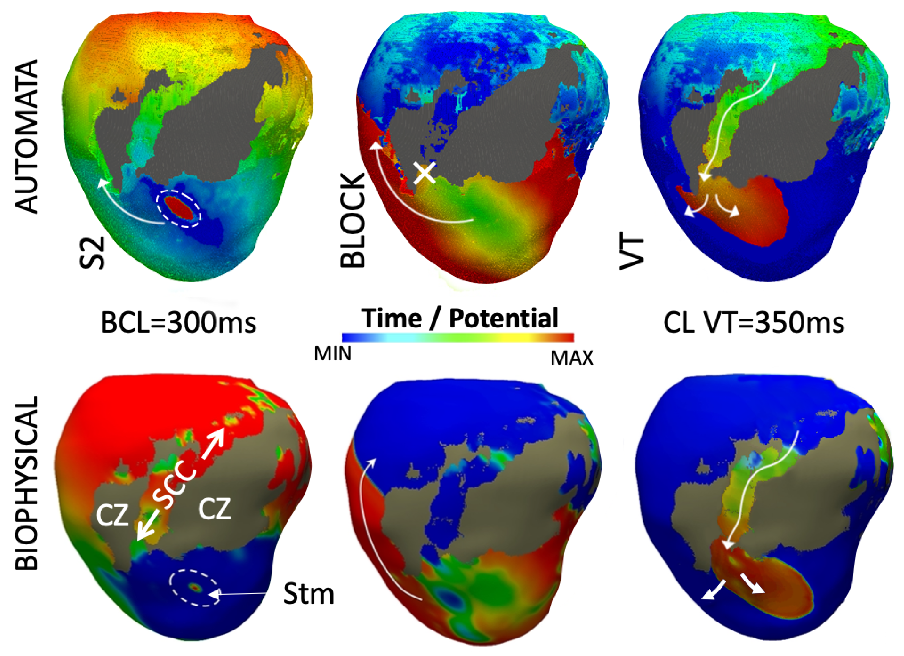
3.4. Simulation of Arrhythmia Dynamics

We performed a study to assess whether it was possible to trigger a ventricular tachycardia in the LV model and reproduce the patient’s monomorphic VT circuit. We replicated the virtual sequential pacing protocol used in the clinics from multiple epicardial locations, as detailed in [5]. The ventricular model included regions of healthy tissue, BZ, and (non-conductive) CZ. To model cellular electrophysiology, we made use of the ten Tusscher model [21], and a modified version for the BZ. We did not include fibroblasts in the BZ or CZ regions. In the CA, changes in the post-infarcted regions were considered in the model by means of specific APDR and CVR curves.

We observed large APD gradients after the model was paced for six stimuli at a BCL of 600 ms (see Figure 8a,b). Spatial variability of APD was observed for both models, with high similarity in the distribution of the heterogeneity. Figure 8c shows the evolution of the APD after each of the first three stimuli for the CA model, where the convergence to a steady APD map can be observed. It can be highlighted that the CA model can predict properly the APD after several heartbeats, and includes models for APD memory and electrotonic effects that are equivalent to the biophysical model. As can be observed, in different regions of the epicardium, there are small ’islands’ due to the electrotonic effect exerted by the underlying tissue (not visible) and the tissue cell heterogeneity present in the BZ.

We induced a VT by applying an S1–S2 protocol in the CA model that mimicked the clinical pace-mapping technique applied to the patient in the EPLab. We virtually paced the LV for 10 cycles (BCL of S1, 600 ms), followed by a single stimulation (BCL of S2, 300 ms) from the epicardial wall (see Figure 9, ‘Stm’). The S2 stimulus resulted in a conduction block at the lower entrance of the SCC, which was composed of BZ tissue (see white cross mark).

Figure 9 shows a comparison of the CA and biophysical simulations at different time instants after the S2 stimulus. In the automaton, colors represent the time remaining until reaching the resting state of each cell in the model. After three cycles, the VT circuit stabilized at a period of 350 ms (see arrow directions), which equals the clinical observation for the patient extracted from the ECG (340 ms).

We measured the improvement obtained in terms of computation time between the CA and the biophysical solver on the high-resolution LV ventricular model. Note that such resolution is not required by the CA, but permitted a fair comparison. CA simulations were performed on a desktop computer (2.9 GHz Intel i5 dual-core, with 8 GB 1867 MHz DDR3), and biophysical simulation on a high-performance computer (64 cores at 2.3 GHz; 4× AMD Opteron 6376 processors). Two complete heartbeats (BCL of = 600 ms) took 76 s in the CA model, which translates into a remarkable cost reduction (×311 faster) compared to 7 h, which corresponds to the use of a biophysical solver using the numerical methods described in previous sections. It is important to acknowledge that implementations based on multi-GPU machines are reducing dramatically the execution time of biophysical simulations [38], although they still require specific hardware and software adapted to its particular architecture, and high-resolution computational meshes.

4. Discussion

Previous studies in the literature have validated biophysical models for cardiac electrophysiology at various levels, from the cellular [39] to tissue and organ levels [18,40], including prospective studies [41,42]. These models can reproduce complex mechanisms that cannot be unveiled in vivo or from animal models, even in the presence of many uncertainties present in the underlying biophysical model. Among the mathematical models and tools to simulate cardiac electrophysiology, we can highlight CARP [43], openCARP [8], openCMISS [44], ELVIRA [6] or CHASTE [7]. All of them include a number of ionic cell models, and allow us to simulate electrical diffusion on tissue using the monodomain and bidomain formulation. They have already gone through benchmarks to assess their accuracy and compare their characteristics [45]. The solvers have been employed to study the mechanistic behavior of cardiac cells, or test different hypotheses related to the pathological functions of cells and tissue.

Since patients who have suffered a myocardial infarction are at lifetime high risk for sudden cardiac death (SCD) [46], there have been proposed several approaches to plan and optimize their treatment. From the clinical perspective, current methods for predicting SCD are based on the LV ejection fraction, but show insufficient clinical accuracy, not identifying many patients at high risk of death. For the particular case of infarct-related VTs, characterization of substrate from MRI scans has started to be employed for SCC detection, and for planning and guiding RFA procedures in patients suffering infarct-related VTs [47,48]. However, mathematical models have been proposed as a valuable tool to plan RFA interventions in patients that suffer from VT, and also to study the risk of SCD in patients that have suffered an infarct.

Cardiac simulations have also been employed to retrospectively plan RFA interventions in patients that suffer from scar-related VT where the optimal ablation target could be estimated [5,18,49,50]. It is worth mentioning a study in which computer simulations were used prospectively to guide the RFA ablation in 21 patients [51]. However, such sophisticated mathematical solutions need highly demanding computational resources and therefore their use in routine clinical practice is still elusive. The alternative solutions are (i) the use of only imaging data to plan the intervention, i.e., to build the 3D computational model of the patient’s heart, including the SCC [47,48], and allowing the electrophysiologists to infer the potential circuits that sustain the arrhythmia; or (ii) the use of fast solvers to carry out the simulations. For the latter, several solvers have been developed that allow faster simulations on GPUs [52,53,54,55], although they still present memory problems due to the size of the computational models, especially for biventricular 3D models. As an alternative, the phenomenological models provide a good balance between accuracy and computational cost that allows their use in clinical environments. Among them, the use of the Eikonal formulation is popular to model tissue diffusion in the absence of a cellular model [56,57,58]. Based on Eikonal, there have been proposed methods to accelerate the solution of Eikonal simulations, such as the multi-front fast marching method, which has been enhanced with restitution properties that would be equivalent to a continuous cellular automaton [59,60]. Similar to our approach, Loewe et al. [60] used a biophysical model to obtain the restitution properties for different cell types and fitted an exponential function to them. In another approach to include dynamic restitution properties, Relan et al. [13] combined Eikonal with minimal cell models [19] and Neic et al. [61] with detailed cell models using the Eikonal reaction approach. Other approaches to reduce the computational time of simulations are based on deep learning, which use neural networks trained with simulations to predict the outcome of the models (Fresca et al. 2020).

Here, we have presented a CA approach that encodes the dynamic properties of cells. Other approaches in the past also made use of CA to accelerate the simulations [62,63,64], and have enhanced them by including restitution properties to extend their use to pathological scenarios [65,66]. Our CA mimics the dynamic properties of a given cellular ionic model, based on biophysical simulations, which allows us to model different types of tissue as a function of the input data. It includes restitution properties at cell and tissue level (APDR and CVR) as in [67,68], as well as cell to cell interaction (electrotonic current) and APD memory [69]. Other studies based on CA models also included the effect of the electrotonic currents by updating the APD as a function of neighboring cells to improve their accuracy compared to biophysical models [70].

All the dynamic data incorporated into our CA model are pre-computed and based on a detailed biophysical model as in [60], improving the performance of the system as it does not need to solve any additional system of equations at the cellular level. Finally, since we were particularly interested in modeling SCC, we included an anatomically based property of cardiac cells known as the safety factor. In simulation scenarios, it could affect the propagation of the wavefront, producing conduction blocks in some SCC scenarios, as observed clinically.

When the goal of the model is to carry out large pace-mapping screenings on the model, CA models could save both computational power and time, to carry out predictions or perform therapy planning prior to an intervention.

The use of CA allows us to obtain a clinically comparable solution to biophysical simulations, with a computational charge suitable to be used in real-time and clinical scenarios. Although the CA simulations still suffer from the same uncertainties as the underlying biophysical model, this novel approach will allow us to reproduce the same clinical scenarios and identify potential personalized therapies, helping to bring realistic electrophysiological simulations to clinical practice.

It is worth mentioning that the CA model can be used to simulate other types of arrhythmias in an efficient way, including focal atrial tachycardia, flutter, atrial fibrillation sustained by rotors, and other types of disorganized ventricular tachycardias that can be triggered from ectopic foci. In all these cases, the combination of heterogeneous tissue and differences in APD can trigger and sustain the arrhythmia, which can be captured by the CA model.

On the downside, among the limitations of the proposed CA, there is the impossibility to simulate certain arrhythmias, such as those triggered by early-after-depolarization (EAD) and delayed-after-depolarization (DAD). Moreover, the model cannot take into account directly the effect of drugs that affect particular ionic channels or structures [71], unless they are previously simulated on a biophysical model, and taken into the CA model library. There are some particular effects, such as the source–sink factors associated with the propagation of curved wavefronts (e.g., rotors), that locally modify the CV that have not been considered in the current implementation of the CA. Our model of SF indirectly incorporates this source–sink factor into the SCC but not when propagation is done in large heterogeneous tissue blocks [72]. In future implementations, heterogeneity in the ventricular tissue propagation could be implemented in the CA as spatial dispersion on the SF parameter, accounting for spatial and directional variability in the conduction properties.

5. Conclusions

We have presented a new tool, a fast CA-based cardiac electrophysiology simulator, to assess the risk of arrhythmia in patients that have suffered a myocardial infarction. We compared the performance and restitution properties obtained from 3D simulations carried out with our CA with respect to a detailed multi-scale biophysical model based on the monodomain formulation and the ten Tusscher ionic cellular model of human ventricular electrophysiology [21]. One of the novelties of this tool, when compared to other CA models, is that it encodes cell dynamic behavior thanks to the consideration of APD and CV restitution properties from a detailed ionic model, which allows us to simulate complex arrhythmic scenarios in 3D, such as spiral waves or ventricular tachycardia.

This CA model can be used to study the vulnerability to VT or SCD among patients that have suffered an infarct, by running thousands of pace-mapping scenarios within a few hours.

References

1. Rudy, Y. From genome to physiome: Integrative models of cardiac excitation. Ann. Biomed. Eng. 2000, 28, 945–950. [Google Scholar] [CrossRef] [PubMed]
2. Lopez-Perez, A.; Sebastian, R.; Ferrero, J.M. Three-dimensional cardiac computational modelling: Methods, features and applications. Biomed. Eng. Online 2015, 14, 35. [Google Scholar] [CrossRef] [PubMed] [Green Version]
3. Niederer, S.A.; Lumens, J.; Trayanova, N.A. Computational models in cardiology. Nat. Rev. Cardiol. 2019, 16, 100–111. [Google Scholar] [CrossRef] [PubMed]
4. Pollard, A.E.; Hooke, N.; Henriquez, C.S. Cardiac propagation simulation. Crit. Rev. Biomed. Eng. 1992, 20, 171–210. [Google Scholar] [PubMed]
5. Lopez-Perez, A.; Sebastian, R.; Izquierdo, M.; Ruiz, R.; Bishop, M.; Ferrero, J.M. Personalized Cardiac Computational Models: From Clinical Data to Simulation of Infarct-Related Ventricular Tachycardia. Front. Physiol. 2019, 10, 580. [Google Scholar] [CrossRef] [PubMed] [Green Version]
6. Heidenreich, E.A.; Ferrero, J.M.; Doblaré, M.; Rodríguez, J.F. Adaptive macro finite elements for the numerical solution of monodomain equations in cardiac electrophysiology. Ann. Biomed. Eng. 2010, 38, 2331–2345. [Google Scholar] [CrossRef] [PubMed]
7. Bernabeu, M.O.; Bordas, R.; Pathmanathan, P.; Pitt-Francis, J.; Cooper, J.; Garny, A.; Gavaghan, D.J.; Rodriguez, B.; Southern, J.A.; Whiteley, J.P. CHASTE: Incorporating a novel multi-scale spatial and temporal algorithm into a large-scale open source library. Philos. Trans. A Math. Phys. Eng. Sci. 2009, 367, 1907–1930. [Google Scholar] [CrossRef]
8. Plank, G.; Loewe, A.; Neic, A.; Augustin, C.; Huang, Y.L.; Gsell, M.A.F.; Karabelas, E.; Nothstein, M.; Prassl, A.J.; Sánchez, J.; et al. The openCARP simulation environment for cardiac electrophysiology. Comput. Methods Programs Biomed. 2021, 208, 106223. [Google Scholar] [CrossRef]
9. Talbot, H.; Marchesseau, S.; Duriez, C.; Sermesant, M.; Cotin, S.; Delingette, H. Towards an interactive electromechanical model of the heart. Interface Focus 2013, 3, 20120091. [Google Scholar] [CrossRef] [Green Version]
10. Trayanova, N.A.; Pashakhanloo, F.; Wu, K.C.; Halperin, H.R. Imaging-Based Simulations for Predicting Sudden Death and Guiding Ventricular Tachycardia Ablation. Circ. Arrhythm. Electrophysiol. 2017, 10, e004743. [Google Scholar] [CrossRef]
11. Trayanova, N.A.; Doshi, A.N.; Prakosa, A. How personalized heart modeling can help treatment of lethal arrhythmias: A focus on ventricular tachycardia ablation strategies in post-infarction patients. Wiley Interdiscip. Rev. Syst. Biol. Med. 2020, 12, e1477. [Google Scholar] [CrossRef] [PubMed]
12. Mendonca Costa, C.; Gemmell, P.; Elliott, M.K.; Whitaker, J.; Campos, F.O.; Strocchi, M.; Neic, A.; Gillette, K.; Vigmond, E.; Plank, G.; et al. Determining anatomical and electrophysiological detail requirements for computational ventricular models of porcine myocardial infarction. Comput. Biol. Med. 2021, 141, 105061. [Google Scholar] [CrossRef] [PubMed]
13. Relan, J.; Chinchapatnam, P.; Sermesant, M.; Rhode, K.; Ginks, M.; Delingette, H.; Rinaldi, C.A.; Razavi, R.; Ayache, N. Coupled personalization of cardiac electrophysiology models for prediction of ischaemic ventricular tachycardia. Interface Focus 2011, 1, 396–407. [Google Scholar] [CrossRef]
14. Pathmanathan, P.; Gray, R.A. Verification of computational models of cardiac electro-physiology. Int. J. Numer. Method Biomed. Eng. 2014, 30, 525–544. [Google Scholar] [CrossRef] [PubMed]
15. Arevalo, H.J.; Vadakkumpadan, F.; Guallar, E.; Jebb, A.; Malamas, P.; Wu, K.C.; Trayanova, N.A. Arrhythmia risk stratification of patients after myocardial infarction using personalized heart models. Nat. Commun. 2016, 7, 11437. [Google Scholar] [CrossRef] [PubMed]
16. McDowell, K.S.; Arevalo, H.J.; Maleckar, M.M.; Trayanova, N.A. Susceptibility to arrhythmia in the infarcted heart depends on myofibroblast density. Biophys. J. 2011, 101, 1307–1315. [Google Scholar] [CrossRef] [Green Version]
17. Corral-Acero, J.; Margara, F.; Marciniak, M.; Rodero, C.; Loncaric, F.; Feng, Y.; Gilbert, A.; Fernandes, J.F.; Bukhari, H.A.; Wajdan, A.; et al. The ‘Digital Twin’ to enable the vision of precision cardiology. Eur. Heart J. 2020, 41, 4556–4564. [Google Scholar] [CrossRef]
18. Chen, Z.; Cabrera-Lozoya, R.; Relan, J.; Sohal, M.; Shetty, A.; Karim, R.; Delingette, H.; Gill, J.; Rhode, K.; Ayache, N.; et al. Biophysical Modeling Predicts Ventricular Tachycardia Inducibility and Circuit Morphology: A Combined Clinical Validation and Computer Modeling Approach. J. Cardiovasc. Electrophysiol. 2016, 27, 851–860. [Google Scholar] [CrossRef] [PubMed] [Green Version]
19. Mitchell, C.C.; Schaeffer, D.G. A two-current model for the dynamics of cardiac membrane. Bull. Math. Biol. 2003, 65, 767–793. [Google Scholar] [CrossRef] [Green Version]
20. Hodgkin, A.L.; Huxley, A.F. A quantitative description of membrane current and its application to conduction and excitation in nerve. J. Physiol. 1952, 117, 500–544. [Google Scholar] [CrossRef]
21. ten Tusscher, K.H.W.J.; Noble, D.; Noble, P.J.; Panfilov, A.V. A model for human ventricular tissue. Am. J. Physiol. Heart Circ. Physiol. 2004, 286, H1573–H1589. [Google Scholar] [CrossRef] [PubMed]
22. Grandi, E.; Pasqualini, F.S.; Bers, D.M. A novel computational model of the human ventricular action potential and Ca transient. J. Mol. Cell. Cardiol. 2010, 48, 112–121. [Google Scholar] [CrossRef] [PubMed] [Green Version]
23. O’Hara, T.; Virág, L.; Varró, A.; Rudy, Y. Simulation of the undiseased human cardiac ventricular action potential: Model formulation and experimental validation. PLoS Comput. Biol. 2011, 7, e1002061. [Google Scholar] [CrossRef] [PubMed] [Green Version]
24. Tomek, J.; Bueno-Orovio, A.; Passini, E.; Zhou, X.; Minchole, A.; Britton, O.; Bartolucci, C.; Severi, S.; Shrier, A.; Virag, L.; et al. Development, calibration, and validation of a novel human ventricular myocyte model in health, disease, and drug block. eLife 2019, 8, e48890. [Google Scholar] [CrossRef] [PubMed]
25. Antzelevitch, C.; Shimizu, W.; Yan, G.X.; Sicouri, S.; Weissenburger, J.; Nesterenko, V.V.; Burashnikov, A.; Di Diego, J.; Saffitz, J.; Thomas, G.P. The M cell: Its contribution to the ECG and to normal and abnormal electrical function of the heart. J. Cardiovasc. Electrophysiol. 1999, 10, 1124–1152. [Google Scholar] [CrossRef]
26. Boyett, M.R.; Jewell, B.R. A study of the factors responsible for rate-dependent shortening of the action potential in mammalian ventricular muscle. J. Physiol. 1978, 285, 359–380. [Google Scholar] [CrossRef] [PubMed]
27. Simurda, J.; Simurdová, M.; Pásek, M.; Bravený, P. Quantitative analysis of cardiac electrical restitution. Eur. Biophys. J. 2001, 30, 500–514. [Google Scholar] [CrossRef]
28. Coveney, S.; Corrado, C.; Oakley, J.E.; Wilkinson, R.D.; Niederer, S.A.; Clayton, R.H. Bayesian Calibration of Electrophysiology Models Using Restitution Curve Emulators. Front. Physiol. 2021, 12, 693015. [Google Scholar] [CrossRef]
29. Cao, J.M.; Qu, Z.; Kim, Y.H.; Wu, T.J.; Garfinkel, A.; Weiss, J.N.; Karagueuzian, H.S.; Chen, P.S. Spatiotemporal heterogeneity in the induction of ventricular fibrillation by rapid pacing: Importance of cardiac restitution properties. Circ. Res. 1999, 84, 1318–1331. [Google Scholar] [CrossRef] [Green Version]
30. Dvir, H.; Zlochiver, S. Stochastic cardiac pacing increases ventricular electrical stability—A computational study. Biophys. J. 2013, 105, 533–542. [Google Scholar] [CrossRef] [Green Version]
31. Tusscher, K.H.T.; Panfilov, A.V. Cell model for efficient simulation of wave propagation in human ventricular tissue under normal and pathological conditions. Phys. Med. Biol. 2006, 51, 6141–6156. [Google Scholar] [CrossRef] [PubMed] [Green Version]
32. Geselowitz, D.B.; Miller, W.T., 3rd. A bidomain model for anisotropic cardiac muscle. Ann. Biomed. Eng. 1983, 11, 191–206. [Google Scholar] [CrossRef] [PubMed]
33. Sethian, J.A. Fast Marching Methods. SIAM Rev. 1999, 41, 199–235. [Google Scholar] [CrossRef]
34. Bueno-Orovio, A.; Cherry, E.M.; Fenton, F.H. Minimal model for human ventricular action potentials in tissue. J. Theor. Biol. 2008, 253, 544–560. [Google Scholar] [CrossRef] [PubMed]
35. Boyle, P.M.; Vigmond, E.J. An intuitive safety factor for cardiac propagation. Biophys. J. 2010, 98, L57–L59. [Google Scholar] [CrossRef] [PubMed] [Green Version]
36. Boyle, P.M.; Franceschi, W.H.; Constantin, M.; Hawks, C.; Desplantez, T.; Trayanova, N.A.; Vigmond, E.J. New insights on the cardiac safety factor: Unraveling the relationship between conduction velocity and robustness of propagation. J. Mol. Cell. Cardiol. 2019, 128, 117–128. [Google Scholar] [CrossRef]
37. Godoy, E.J.; Lozano, M.; García-Fernández, I.; Ferrer-Albero, A.; MacLeod, R.; Saiz, J.; Sebastian, R. Atrial fibrosis hampers non-invasive localization of atrial ectopic foci from multi-electrode signals: A 3d simulation study. Front. Physiol. 2018, 9, 404. [Google Scholar] [CrossRef] [Green Version]
38. Gouvêa de Barros, B.; Sachetto Oliveira, R.; Meira, W., Jr.; Lobosco, M.; Weber dos Santos, R. Simulations of complex and microscopic models of cardiac electrophysiology powered by multi-GPU platforms. Comput. Math. Methods Med. 2012, 2012, 824569. [Google Scholar] [CrossRef] [Green Version]
39. Yang, P.C.; DeMarco, K.R.; Aghasafari, P.; Jeng, M.T.; Dawson, J.R.; Bekker, S.; Noskov, S.Y.; Yarov-Yarovoy, V.; Vorobyov, I.; Clancy, C.E. A computational pipeline to predict cardiotoxicity: From the atom to the rhythm. Circ. Res. 2020, 126, 947–964. [Google Scholar] [CrossRef]
40. Maleckar, M.M.; Myklebust, L.; Uv, J.; Florvaag, P.M.; Strøm, V.; Glinge, C.; Jabbari, R.; Vejlstrup, N.; Engstrøm, T.; Ahtarovski, K.; et al. Combined In-silico and Machine Learning Approaches Toward Predicting Arrhythmic Risk in Post-infarction Patients. Front. Physiol. 2021, 12, 745349. [Google Scholar] [CrossRef]
41. Zhou, S.; AbdelWahab, A.; Sapp, J.L.; Sung, E.; Aronis, K.N.; Warren, J.W.; MacInnis, P.J.; Shah, R.; Horáček, B.M.; Berger, R.; et al. Prospective Multicenter Assessment of a New Intraprocedural Automated System for Localizing Idiopathic Ventricular Arrhythmia Origins. JACC Clin. Electrophysiol. 2021, 7, 395–407. [Google Scholar] [CrossRef] [PubMed]
42. Zhou, S.; AbdelWahab, A.; Horáček, B.M.; MacInnis, P.J.; Warren, J.W.; Davis, J.S.; Elsokkari, I.; Lee, D.C.; MacIntyre, C.J.; Parkash, R.; et al. Prospective Assessment of an Automated Intraprocedural 12-Lead ECG-Based System for Localization of Early Left Ventricular Activation. Circ. Arrhythm. Electrophysiol. 2020, 13, e008262. [Google Scholar] [CrossRef] [PubMed]
43. Vigmond, E.J.; Hughes, M.; Plank, G.; Leon, L.J. Computational tools for modeling electrical activity in cardiac tissue. J. Electrocardiol. 2003, 36 (Suppl. 1), 69–74. [Google Scholar] [CrossRef] [PubMed]
44. Bradley, C.; Bowery, A.; Britten, R.; Budelmann, V.; Camara, O.; Christie, R.; Cookson, A.; Frangi, A.F.; Gamage, T.B.; Heidlauf, T.; et al. OpenCMISS: A multi-physics & multi-scale computational infrastructure for the VPH/Physiome project. Prog. Biophys. Mol. Biol. 2011, 107, 32–47. [Google Scholar] [CrossRef] [PubMed]
45. Niederer, S.A.; Kerfoot, E.; Benson, A.P.; Bernabeu, M.O.; Bernus, O.; Bradley, C.; Cherry, E.M.; Clayton, R.; Fenton, F.H.; Garny, A.; et al. Verification of cardiac tissue electrophysiology simulators using an N-version benchmark. Philos. Trans. A Math. Phys. Eng. Sci. 2011, 369, 4331–4351. [Google Scholar] [CrossRef] [Green Version]
46. Adabag, A.S.; Therneau, T.M.; Gersh, B.J.; Weston, S.A.; Roger, V.L. Sudden death after myocardial infarction. JAMA 2008, 300, 2022–2029. [Google Scholar] [CrossRef] [Green Version]
47. Fern’andez-Armenta, J.; Berruezo, A.; Andreu, D.; Camara, O.; Silva, E.; Serra, L.; Barbarito, V.; Carotenutto, L.; Evertz, R.; Ortiz-P’erez, J.T.; et al. Three-dimensional architecture of scar and conducting channels based on high resolution ce-CMR: Insights for ventricular tachycardia ablation. Circ. Arrhythm. Electrophysiol. 2013, 6, 528–537. [Google Scholar] [CrossRef] [Green Version]
48. Soto-Iglesias, D.; Penela, D.; J’auregui, B.; Acosta, J.; Fern’andez-Armenta, J.; Linhart, M.; Zucchelli, G.; Syrovnev, V.; Zaraket, F.; Ter’es, C.; et al. Cardiac Magnetic Resonance-Guided Ventricular Tachycardia Substrate Ablation. JACC Clin. Electrophysiol. 2020, 6, 436–447. [Google Scholar] [CrossRef]
49. Arevalo, H.; Plank, G.; Helm, P.; Halperin, H.; Trayanova, N. Tachycardia in post-infarction hearts: Insights from 3D image-based ventricular models. PLoS ONE 2013, 8, e68872. [Google Scholar] [CrossRef] [Green Version]
50. Deng, D.; Prakosa, A.; Shade, J.; Nikolov, P.; Trayanova, N.A. Characterizing Conduction Channels in Postinfarction Patients Using a Personalized Virtual Heart. Biophys. J. 2019, 117, 2287–2294. [Google Scholar] [CrossRef]
51. Prakosa, A.; Arevalo, H.J.; Deng, D.; Boyle, P.M.; Nikolov, P.P.; Ashikaga, H.; Blauer, J.J.E.; Ghafoori, E.; Park, C.J.; Blake, R.C., 3rd; et al. Personalized virtual-heart technology for guiding the ablation of infarct-related ventricular tachycardia. Nat. Biomed. Eng. 2018, 2, 732–740. [Google Scholar] [CrossRef] [PubMed]
52. Vigmond, E.J.; Boyle, P.M.; Leon, L.; Plank, G. Near-real-time simulations of biolelectric activity in small mammalian hearts using graphical processing units. Annu. Int. Conf. IEEE Eng. Med. Biol. Soc. 2009, 2009, 3290–3293. [Google Scholar] [CrossRef] [PubMed] [Green Version]
53. Vigueras, G.; Roy, I.; Cookson, A.; Lee, J.; Smith, N.; Nordsletten, D. Toward GPGPU accelerated human electromechanical cardiac simulations. Int. J. Numer. Method Biomed. Eng. 2014, 30, 117–134. [Google Scholar] [CrossRef] [PubMed] [Green Version]
54. Sachetto Oliveira, R.; Martins Rocha, B.; Burgarelli, D.; Meira, W., Jr.; Constantinides, C.; Weber Dos Santos, R. Performance evaluation of GPU parallelization, space-time adaptive algorithms, and their combination for simulating cardiac electrophysiology. Int. J. Numer. Method Biomed. Eng. 2018, 34, e2913. [Google Scholar] [CrossRef]
55. Garcia-Molla, V.M.; Liberos, A.; Vidal, A.; Guillem, M.S.; Millet, J.; Gonzalez, A.; Martinez-Zaldivar, F.J.; Climent, A.M. Adaptive step ODE algorithms for the 3D simulation of electric heart activity with graphics processing units. Comput. Biol. Med. 2014, 44, 15–26. [Google Scholar] [CrossRef] [Green Version]
56. Pashaei, A.; Romero, D.; Sebastian, R.; Camara, O.; Frangi, A.F. Fast multiscale modeling of cardiac electrophysiology including Purkinje system. IEEE Trans. Biomed. Eng. 2011, 58, 2956–2960. [Google Scholar] [CrossRef]
57. Cedilnik, N.; Duchateau, J.; Dubois, R.; Sacher, F.; Jaïs, P.; Cochet, H.; Sermesant, M. Fast personalized electrophysiological models from computed tomography images for ventricular tachycardia ablation planning. Europace 2018, 20, iii94–iii101. [Google Scholar] [CrossRef] [PubMed]
58. Quaglino, A.; Pezzuto, S.; Koutsourelakis, P.S.; Auricchio, A.; Krause, R. Fast uncertainty quantification of activation sequences in patient-specific cardiac electrophysiology meeting clinical time constraints. Int. J. Numer. Method Biomed. Eng. 2018, 34, e2985. [Google Scholar] [CrossRef]
59. Sermesant, M.; Konukoglu, E.; Delingette, H.; Coudiere, Y.; Chinchapatnam, P.; Rhode, K.S.; Razavi, R.; Ayache, N. An anisotropic multi-front fast marching method for real-time simulation of cardiac electrophysiology. In Proceedings of the International Conference on Functional Imaging and Modeling of the Heart, Salt Lake City, UT, USA, 7–9 June 2007; pp. 160–169. [Google Scholar]
60. Loewe, A.; Poremba, E.; Oesterlein, T.; Luik, A.; Schmitt, C.; Seemann, G.; Dössel, O. Patient-Specific Identification of Atrial Flutter Vulnerability-A Computational Approach to Reveal Latent Reentry Pathways. Front. Physiol. 2018, 9, 1910. [Google Scholar] [CrossRef] [Green Version]
61. Neic, A.; Campos, F.O.; Prassl, A.J.; Niederer, S.A.; Bishop, M.J.; Vigmond, E.J.; Plank, G. Efficient computation of electrograms and ECGs in human whole heart simulations using a reaction-eikonal model. J. Comput. Phys. 2017, 346, 191–211. [Google Scholar] [CrossRef]
62. Saxberg, B.E.; Cohen, R.J. Cellular automata models for reentrant arrhythmias. J. Electrocardiol. 1990, 23, 95. [Google Scholar] [CrossRef]
63. Siregar, P.; Sinteff, J.P.; Julen, N.; Le Beux, P. An interactive 3D anisotropic cellular automata model of the heart. Comput. Biomed. Res. 1998, 31, 323–347. [Google Scholar] [CrossRef] [PubMed]
64. Werner, C.; Sachse, F.; Dössel, O. Electrical excitation propagation in the human heart. Int. J. Bioelectromagn. 2000, 2, 96–117. [Google Scholar]
65. Zhu, H.; Sun, Y.; Rajagopal, G.; Mondry, A.; Dhar, P. Facilitating arrhythmia simulation: The method of quantitative cellular automata modeling and parallel running. Biomed. Eng. Online 2004, 3, 29. [Google Scholar] [CrossRef] [Green Version]
66. Sabzpoushan, S.H.; Pourhasanzade, F. A Cellular Automata-based Model for Simulating Restitution Property in a Single Heart Cell. J. Med. Signals Sens. 2011, 1, 19–23. [Google Scholar]
67. Corrado, C.; Zemzemi, N. A conduction velocity adapted eikonal model for electrophysiology problems with re-excitability evaluation. Med. Image Anal. 2018, 43, 186–197. [Google Scholar] [CrossRef] [Green Version]
68. Ai, W.; Patel, N.D.; Roop, P.S.; Malik, A.; Trew, M.L. Cardiac Electrical Modeling for Closed-Loop Validation of Implantable Devices. IEEE Trans. Biomed. Eng. 2020, 67, 536–544. [Google Scholar] [CrossRef] [PubMed]
69. Bueno-Orovio, A.; Hanson, B.M.; Gill, J.S.; Taggart, P.; Rodriguez, B. In vivo human left-to-right ventricular differences in rate adaptation transiently increase pro-arrhythmic risk following rate acceleration. PLoS ONE 2012, 7, e52234. [Google Scholar] [CrossRef] [Green Version]
70. Campos, R.S.; Silva, J.G.R.; Barbosa, H.J.C.; Santos, R.W.d. Electrotonic Effect on Action Potential Dispersion with Cellular Automata. In Proceedings of the International Conference on Computational Science and Its Applications, Cagliari, Italy, 1–4 July 2020; pp. 205–215. [Google Scholar]
71. Dux-Santoy, L.; Sebastian, R.; Felix-Rodriguez, J.; Ferrero, J.M.; Saiz, J. Interaction of specialized cardiac conduction system with antiarrhythmic drugs: A simulation study. IEEE Trans. Biomed. Eng. 2011, 58, 3475–3478. [Google Scholar] [CrossRef]
72. Ciaccio, E.J.; Coromilas, J.; Wit, A.L.; Peters, N.S.; Garan, H. Source-Sink Mismatch Causing Functional Conduction Block in Re-Entrant Ventricular Tachycardia. JACC Clin. Electrophysiol. 2018, 4, 1–16. [Google Scholar] [CrossRef]
Figure 1. Restitution curves obtained from 3D biophysical simulations based on ten Tusscher model [21]. (a) displays APD restitution curves for the three cell types (endocardial, midmyocardial, epicardial) in healthy (solid lines) and pathological conditions (BZ, dashed lines). (b) CV restitution curves for the same types of cells, together with the 3D slab model used to perform all the biophysical simulations and measurements and with the location of the probes. Red color represents activated tissue, and blue color shows tissue in resting state.
Mathematics 10 01293 g001
Figure 2. The activation time for a node is computed assuming a plane activation wavefront. Under this assumption, the activation time t k a for node k can be computed from the average location of its activating neighbor points p ¯ k and their average activation time t ¯ k as t k a = t ¯ k + d ( p ¯ k , p k ) / v k .
Mathematics 10 01293 g002
Figure 3. Safety factor based on anatomical disposition of tissue for a regular 2D grid. On the left, there is an example showing how to calculate SF for node i, as a ratio between healthy (white) and pathological (gray) tissue. On the right, there is an SCC with the SF calculated for each cell, showing a conduction block at the exit of the channel (red line), since transition from 8/16 to 10/16 cannot proceed.
Mathematics 10 01293 g003
Figure 4. Comparison of activation time maps for biophysical and CA simulations. Results from simulation of a flat wavefront originating from the bottom of the 3D slab model and progressing in the Y-direction. Models are labeled as a function of the methods used to solve the electrical diffusion (biophysical or CA), and the resolution of the hexahedral elements ( 300 μ m to 1200 μ m). Colors represent the time in which a node activates from 0 to 77 ms.
Mathematics 10 01293 g004
Figure 5. Comparison of electrical propagation in a 3D slab of tissue for biophysical and CA models. The maps in the first and second columns represent the local activation maps in milliseconds produced by a single stimulus in the center of the model. Third row shows the difference between biophysical and CA simulations. Mesh is 5 × 5 cm in size and has an element resolution of 300 μ m.
Mathematics 10 01293 g005
Figure 6. Comparative of simulated rotor spiral waves using a CA and a biophysical model in a slab of tissue. Simulations are shown for 240 ms consecutive time instants after the rotor stabilized. CA simulation is color-coded by time in milliseconds (ms) from the activation (red tones) to the resting state (blue tones). Biophysical simulation shows the equivalent simulation, where colors represent transmembrane potential in millivolts (mV).
Mathematics 10 01293 g006
Figure 7. Effect of safety factor on wavefront propagation for channels with different widths. The 3D slab tissue model of several layers containing a conduction channel in the inner layers, healthy tissue (blue), BZ tissue (light gray), and CZ (red); see right legend. Top row corresponds to CA simulations, while bottom row is for biophysical simulations. Columns correspond to an SCC of different width. As observed for an SCC smaller than 0.9 × 0.9 mm, there is a conduction block. Elements in the model are hexahedral of 0.3 mm.
Mathematics 10 01293 g007
Figure 8. APD maps on the epicardial surface. APD map after S1 pacing protocol (BCL = 600 ms) for (a) biophysical simulation and (b) CA simulation. (c) shows the evolution of the APD after each of the first three stimuli for the CA model. Color represents the APD at each node. CZ is depicted in gray color.
Mathematics 10 01293 g008
Figure 9. Simulation time instants (ms) for CA and biophysical model. VT episode resulted from applying an S1–S2 protocol at the location labeled as ’Stm’. First row shows the endocardial layer (light gray) and the activity in the BZ region in the CA model (CZ and healthy tissue are transparent), while second row shows the equivalent in the biophysical model with all tissue types visible (CZ in dark gray color). Colors in the CA simulation represent time (ms), and in the biophysical simulation represent potential (mV). A conduction block can be observed a few milliseconds after the S2 (white cross). VT is subsequently sustained across the SCC. White arrows show the direction of the wavefront.
Mathematics 10 01293 g009
Publisher’s Note: MDPI stays neutral with regard to jurisdictional claims in published maps and institutional affiliations.