1. Introduction
The world energy system is undoubtedly in transition. The widespread adoption and use of renewable energy is key to fighting climate change and ensuring a sustainable future. According to WindEurope [
1], the European Commission’s forecasts demonstrate that renewable-based electricity will be critical to achieving climate neutrality in Europe by 2050. This will need wind accounting for 50% of the EU’s power mix, with renewables accounting for 81%. To accomplish this target, offshore wind is a crucial component as it offers higher and steadier wind speeds and vast possibilities for their placement (easy to find new locations compared to on-shore).
The crux of the matter in the advancement of the offshore wind industry is the reduction in the levelized cost of energy, and a key factor to accomplishing it is through the optimization of the inspection and maintenance strategies. In particular, structural health monitoring (SHM) of the support structure has an added value, estimated to be between 1.93–18.11 M€, see [
2]. An effective structural integrity management of offshore wind farm assets could reduce the number of inspections they need during their lifetime. SHM has been widely applied to civil infrastructures [
3], such as bridges, but there is a research gap in the area when being applied to hazardous environments, such as the ones where support structures of offshore wind turbines (WT) are installed. On the one hand, in this complex environment, the data suffer from noise measurement that must be removed in deep learning methods. Noise reduction in the data are crucial and can be accomplished, for example, by a Savitzky–Golay filter and wavelet decomposition, e.g., [
4]. On the other hand, WTs are placed in a marine environment, subject to potential extreme winds, waves, and currents, which can change rapidly and are initially unknown. Related to the main challenges of SHM in offshore foundations, as stated in [
5]: “A defining marine environment main characteristic is that structures are always subject to excitations. Techniques for structural health monitoring, vibration, and data analysis must be capable of coping with such ambient excitations. As the input is typically not known, a normal input–output formalism cannot be used”. That is, the standard SHM approach based on guided waves (where the input excitation is known and imposed to the structure and then the output vibration is measured), widely used in many areas such as aeronautics [
6], cannot be applied in a straightforward manner to offshore WTs; as the excitation is not known (wind, waves, currents), neither can be imposed. Thus, an output-only approach is imperative.
A new paradigm, a vibration-response-only methodology, must be developed that assumes unknown input excitations and that only the vibration response is measurable by means of different sensors (accelerometers or fiber Bragg grating, for instance). In recent years, interest in this type of methodology has grown. For example, in [
7], parametric reduced order models for cracked shells are developed and applied to crack detection problems, and an output-only scheme is adopted based on transmissibility functions. It is also noteworthy that the vibration-response-only approach for a jacket structure in [
8] where a comprehensive and critical assessment of the diagnostic performance of five prominent response-only methods is presented based on incipient, ‘minor’ to ‘mild’, damages on a lab-scale wind turbine jacket structure. In [
9], an SHM method for floating offshore WTs was tested using operational modal analysis. The results showed that the curvature mode shape was the most effective modal property to detect damage location and intensity. Likewise, Ref. [
10] contributed an SHM system for real tripod WT supports based on fiber Bragg grating (FBG) sensors to detect and localize the damage. A meaningful work was presented in [
11], where a time–frequency analysis is proposed based on single mode function decomposition to overcome the mode-mixing problem. Finally, some publications using the same test bench as the one used in this study are: [
12], where the SHM for jacket foundations is stated via a signal-to-image conversion of the accelerometer data into multichannel images and convolutional neural networks, combined with synthetic data augmentation; Ref. [
13] that proposes the fractal dimension as a suitable feature to identify and classify different types of damage; and Ref. [
14], where structural damage classification is achieved by using principal component analysis and extreme gradient boosting. It is noteworthy that, in contrast to all aforementioned references, where large datasets with faulty data are available (or synthetic data need to be generated); in this work, Siamese neural networks (SNNs) are used, taking advantage of their ability to learn from very little data. Furthermore, most of the aforementioned references only detect one specific type of damage but do not face the challenge of detecting and classifying different types of damage, which is accomplished in this study.
SNNs are made up of two identical artificial neural networks that function in parallel and compare their outputs at the end, typically using a distance metric. The output of the SNNs execution may be thought of as a semantic similarity between the projected representations of the two input vectors. The ability to learn from very little data has made SNNs more popular in recent years, being applied in a wide variety of applications. For example, in [
15], SNNs are employed in differential lung diagnoses with CT scans as a key element of the proposed approach to facilitate the implementation of explainable artificial intelligence systems. In [
16], they are proposed to identify cyber-physical attacks dealing with the problem of few labeled data and to alleviate the over-fitting issue while enhancing accuracy. In [
17], robust and discriminative gait features for human identification are automatically extracted based on SNNs and limited training data. However, to the best of the authors’ knowledge, SNNs have not yet been used in the area of damage detection and/or diagnosis. In this work, two in cascade Siamese convolutional neural networks are proposed to detect and classify the faults under study.
This work contributes a vibration-response-only SHM methodology for jacket type support structures in offshore WTs, based on convolutional SNNs. In contrast to standard SNNs, which are feedforward neural networks [
18], this is proposed to introduce convolutional layers. To avoid the traditional complex feature extraction processes that appear in machine learning approaches [
19], this study advises utilizing deep convolutional SNNs. Thus, the initial raw accelerometer data will be converted into gray-scale multichannel images, and then features will be automatically extract by the deep convolutional SNNs. The methodology then follows the subsequent steps: (i) Vibration data are acquired, (ii) conversion of the dataset to multichannel gray-scale images, (iii) a first convolutional SNN discerns between healthy and damaged structural states, and a second convolutional SNN classifies the samples, detected as damaged by the first network, between crack or unlocked bolt types of damage. In a nutshell, the contributions of the proposed methodology that should be highlighted are:
It is based only on the output vibration data gathered by accelerometer sensors (the excitation given by the wind is assumed to be unknown). Thus, it is a vibration-response-only methodology.
It achieves damage detection and, in case damage is detected, damage type classification based on two in-cascade Siamese convolutional neural networks.
It works under all regions of operation of the wind turbine.
It needs little data to be trained, as it is based on Siamese convolutional neural networks that have the ability to learn from very little data in comparison to standard machine learning approaches.
It is tested in a downscaled experimental laboratory structure.
The performance indicators show all results above 96%.
The following is the paper’s outline. The experimental down-scaled setup is introduced in
Section 2.
Section 3 details the proposed strategy. Finally, findings are discussed in
Section 4, and conclusions are derived in
Section 5.
2. Laboratory Setup
The configuration of the experimental test bench is detailed in
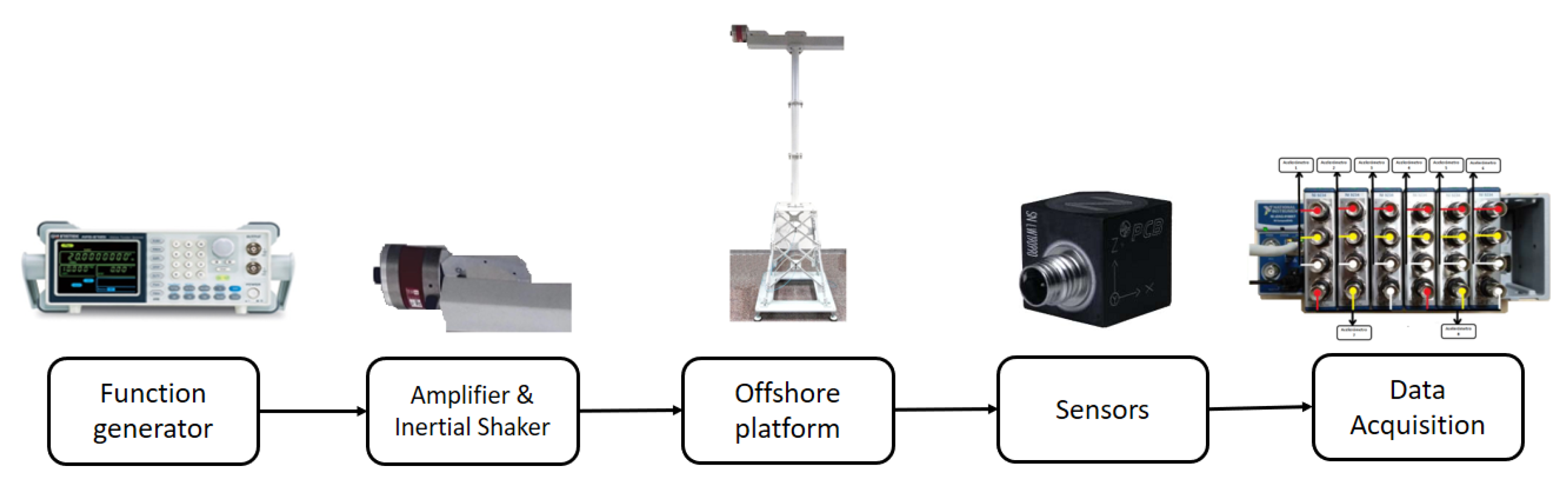
Figure 1. The process begins with the white noise signal obtained by the function generator model GW INSTEK AF-2005. The generated signal is amplified and enters the inertial shaker model Data Physics GW-IV47, located in the upper side of the scale turbine structure, which simulates gusts of wind. The vibrations produced by the wind gust simulation are directly related to the amplitude of white noise, which has factors of 0.5, 1, 2, and 3. Vibration monitoring is carried out using eight triaxial accelerometers (PCB R Piezotronic, model 356A17), positioned as shown in
Figure 2 (right); there are 24 vibration signals. The sensors are linked up to six National InstrumentsTM cartridges (model NI 9234) that are attached to the National Instruments cDAQ-9188 chassis.
The structure itself is 2.7 m high and divided into three sections (see
Figure 2 (left)) shown below.
The upper section is composed of a bar one meter long and 0.6 m wide; here, the wind turbine nacelle and the wind speed are simulated using the agitator and different excitation signals.
The central section is made up of a tower divided into three parts and bolted together.
Finally, at the bottom is the jacket section, which is made up of 32 S275JR steel bars, DC01 LFR steel sheets, and components like screws and nuts. All sections are screwed in with a torque of 12 Nm.
The approach of the proposed strategy is that it must be able to detect and classify the types of damage studied, as well as be robust enough to replace a bar with a new healthy one (avoiding false alarms). The following structural states are presented:
Figure 3 shows the different structural states in detail.
The down-scaled laboratory structure is a simplified but valid model for the practical study of this work, which aims to be a proof of concept for the detection and diagnosis of damaged bars in jacket-type platforms. This is demonstrated by the fact that similar laboratory structures have been previously used in the literature for this aim, such as [
8] and [
12].
3. Methodology
The suggested methodology’s stages are all listed below. First, the raw data from the sensors are collected. Second, an exploratory data analysis process is carried out to validate the hypothesis of this research. Then, the data are pre-processed to obtain a 24-channel image dataset. Subsequently, the data are reshaped and divided to be later entered into the first convolutional SNN. Then, the images classified as damaged are introduced to a second convolutional SNN to classify the damage between the crack or unlocked bolt types. Next, subsections comprehensively draw the above-mentioned different stages.
3.1. Data Acquisition
Each experimental test lasts 60 s with an approximate sampling frequency of 275.27 Hz. As a result, 16,516 measurements were obtained from each of the 24 sensors (24 vibration signals). Twenty-five experimental tests were carried out for each of the white noise (WN) amplitudes (0.5, 1, 2, and 3), obtaining a total of 100 experiments. The experiments performed for each amplitude are detailed below:
10 tests with the original bar;
5 tests with the replica bar;
5 tests with a bar damaged by a 5 mm crack;
5 tests with an unlocked bolt damage.
Table 1 presents the number of experiments for each structural state and associated white noise amplitude factor.
Table 2 shows the data obtained from each experimental test. The number of timestamps (16516) determine the number of rows, and the number of columns reflect the number of sensors. Take note that the data in the first column is connected to sensor A, the data in the second column is related to sensor B, and so on and so forth, until all 24 available sensors are covered.
3.2. Exploratory Data Analysis
Exploratory data analysis is essential to fully comprehend the information available from the data, and it is very useful when it comes to obtaining insights from the available data. The role of this process is to explore all the data to answer questions that help validate the hypotheses raised [
20].
In this work, the following concern is stated: How does the distribution of each sensor signal, associated with a specific state, perform with different white noise amplitude factors? For this, after the data collection process is implemented, data visualization is created via a histogram.
As can be observed in
Figure 4, there are four plots. On each of these plots, the statistical distributions for each state (healthy, replica, crack and unlocked bolt) are shown. On the upper left plot, where the white noise amplitude factor is small (0.5), it can be noted that the statistical distributions of the default state and the replica state (henceforth called healthy pair) are similar, as their centers tend to the plot’s right side. Moreover, the statistical distributions of the crack state and the unlocked bolt state (henceforth called faulty pair) are similar to each other, but their centers tend to the plot’s left side.
In the upper right of the plot, where the white noise amplitude factor is mid-low (1), it can be seen that the healthy pair and faulty pair statistical distributions still maintain a similarity to each other. However, the similarity differs among the pairs, where the centers of the healthy pair and the faulty pair are close to the right and left of the plot, respectively. At the lower left plot, where the white noise amplitude factor is mid-high (2), it can be observed that the pairs of distributions are almost similar to each other—however, with a slight level of difference. Finally, for the lower right plot, where the white noise amplitude factor is high (3), it can be noted that the distribution pairs, healthy and faulty, are almost indistinguishable due to the overlay behavior of each individual distribution. Taking into account that the different applied white noise amplitude factors represent different wind-speed regions of operation of the wind turbine, it may be stated that, at greater wind speeds (region where WTs intended to run the majority of the time), distinguishing whether a sample belongs to a given structural state becomes more challenging.
3.3. Data Preprocessing: Reshape
In this section, a feature engineering technique, data reshaping, is applied to ensure that each one of the samples to be processed by the SNNs have sufficient information from each sensor to determine the state of the structure. Initially, each experiment had 24 columns and 16,516 rows, representing the source of the data (sensors) and the data acquired over time, respectively (see
Table 2).
In this study, images (samples) that contain the information of approximately one second of data are created. Recall that the sample rate is 275.27 Hz. Thus, the first 256 values from each column (approximately one second of data) were reshaped into 16 × 16 matrices. Then, the next 256 values from each column were reshaped into 16 × 16 matrices, and so on, as can be seen in
Figure 5 and
Figure 6. At the end, the final target images’ shapes were 16 × 16 for each sensor. Note that, in
Figure 5 and
Figure 6, the values A
i, B
i, ⋯, X
i are measurements of the different sensors that correspond to the same time step—that is, acquired at the same time instant. In other words, in general, A
i, B
i, …, and X
i all correspond to the same time step
i.
The last 132 values from each column were not considered because they could not complete the 256 values required to build a (16 × 16) matrix. Once the two-dimensional matrices were obtained, the process was continued with the creation of the 16 × 16 × 24 size images. For each experiment, the first matrices formed by the 256 first values of their respective columns were time-related. Meaning that each value from a specific position on each matrix was sampled at the same time as the values occupying the same position on the rest of the 23 matrices. Basically, the first 24 matrices were grouped together to maintain this relation provided by this new feature. The same was applied to the second group of matrices, and so on and so forth, until 64 groups of matrices were obtained from each experiment (see
Figure 7).
At the end of the process, 1280 images were obtained from each of the replica bar, cracked, and unlocked bolt bar experiments, while 2560 images were obtained from the healthy bar experiments.
3.4. Data Split: Train, Validation, and Test Sets
For the data split process, 80 percent of the data was considered for the training set, 10 percent of the data for the validation set, and the remaining 10 percent was put on hold to be used only for testing. This applies to both the damage detection and the damage diagnosis SNN models. For the damage detection SNN, the data were grouped in such a way that the healthy and the replica structure state images were grouped into the first class (healthy), while the crack and the unlocked bolt structure state images were grouped into the second class (faulty). On the other hand, for the damage diagnosis SNN, the data were grouped into following two classes: crack structural state and unlocked bolt structural state.
Once the images were in their assigned classes, various subsets were created in order to separate the images, as per the structural state and white noise level. After this process, the following subsets were obtained per state: white noise level of 0.5, white noise level of 1, white noise level of 2, and white noise level of 3. Finally, recall that 80, 10, and the remaining 10 percent of each one of the obtained subsets are used in the training, validation, and test set, respectively. Thus, a data balance is ensured per structural state and white noise level, as can be seen in
Table 3 and
Table 4.
3.5. Siamese Neural Network (SNN)
The SNN algorithm was developed by Bromley et al. [
21] in 1994 to verify signatures written on a touch-sensitive pad. The SNNs consist of two identical neural network architectures capable of learning and extracting the hidden representation of their respective inputs [
18].
In this work, the two neural networks are both convolutional neural networks [
22] and employ back-propagation during training [
23]. The basic idea of this methodology is that both networks work in parallel and finally compare their outputs. The comparison function is the Euclidean distance. The output generated by an SNN execution can be considered the semantic similarity between the projected representation of the two input matrices [
24].
Two models were deployed for the damage detection and diagnosis problems to compare their performance. The first model (model 1) consisted of an SNN with a feature extraction stage of one convolutional layer (see
Figure 8), while the second model (model 2) implemented two convolutional layers in its feature extraction stage (see
Figure 9). The rest of this section details each step in the methodology:
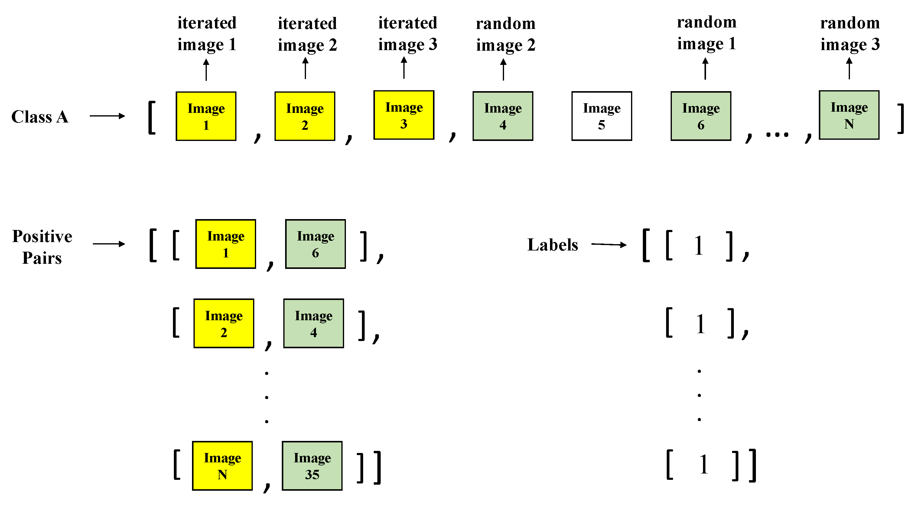
Image pair creation Stage: The SNN has a pair of images input, where this pair can be positive or negative. A positive pair consists of two images that belong to the same class, while a negative pair consists of two images from different classes [
25]. For the training, validation, and test sets, positive and negative pairs were created. For explanation, the two classes are noted as class A and class B. First, an empty array for the pair of images is set as well as an empty array of labels, which help to indicate by index if a pair of images (from the pair of images array) is positive (1) or negative (0). Next, an iterative process is performed through the set of images that belong to class A. For each image, a random image is selected from the same class. Next, a positive pair is created by the image that is being iterated, and the random image selected from the same class (this pair is added to the image pair array). Then, a label with the value of one is added to the labels array previously created, so the image pair added, and the label are related by position through both of the arrays. This process can be observed in
Figure 10.
For the creation of negative pairs, a similar process is carried out, but the random image is chosen from class B. Then, a label with the value of 0 is added to the labels array previously created in order to maintain the index relation between the pair and the label. This iterative process is carried out also for class B (the negative image comes from class A and positive image comes from class B), so it can be ensured that all the images are used. This process can be observed in
Figure 11.
If the sets of images are not of the same length, then the difference is resolved by iterating a quantity of images equal to this difference on the lower length set. At the end, a set
X is composed by
N sample pairs
, which are two images from the same or different classes. Remember, for both creations’ processes (positive and negative), both states’ groups in each case are used. For example, for the damage detection stage, first, the healthy and replica images are used as class A and positive pairs are created. Then, the other group class (crack and unlocked bolt) is used as class A, and the other positive pairs are created. The same process is used for the negative pairs creation and the damage diagnosis stage.
Table 5 and
Table 6 detail the number of image pairs used for training, validation, and test datasets.
Input Stage: In the proposed methodology, two two-dimensional CNNs are used to extract hidden representation (spatial feature vectors), so the input is the matrix mentioned in
Section 3.3, in the shape of
.
Feature extraction: A Siamese network architecture is employed at this stage to extract features from the input sample pairs. The Siamese network is made up of two identical CNNs with the same network topology and one fully connected layer at the end.
Table 7 and
Table 8 indicate the different feature extraction layers, their configurations, and their dimensions for the two studied models noted as model 1 (shallow NN with only one CNN layer) and model 2 (NN with two CNN layers).
Similarity measurement: The output vectors obtained from both fully connected layers are introduced to a new function layer to compute the similarity (distance) between them. This process can be carried out by metrics such as Euclidean distance, cosine distance, or Manhattan distance [
26] because it highlights the geometric differences between two elements. In this work, the Euclidean distance is used as the similarity matrix. The similarity between the input vectors is calculated by the formula
where
represents the feature vector obtained by one of the CNNs,
x refers to the input, and
k denotes the
k-th sample for a pair
.
Output stage: After the similarity is calculated, this value enters a last fully connected layer to convert it to a similarity scalar value .
Because the idea is to calculate a similarity probability between 0 and 1, a sigmoid function is used as activation function
where
is the sigmoid function [
27]
Note that is a value between 0 and 1. The closer this value is to 1, the greater the probability that the two matrices are of the same class. Likewise, the closer this value is to zero, the lower the probability that the two matrices are of the same class.
Hyperparameters: The SNNs are configured with the following hyperparameters’ selection. The Adams optimizer with learning rate 0.05, = 0.9, = 0.999, is used. The used cost function is the binary cross entropy, and the batch size is set to 32. Hyperparameter tuning did not change the obtained results much, except for the value of the learning rate, where lower values improved the accuracy.
4. Results
To recognize whether a model is overfitting, the loss curves of the training set and the validation set are first presented. Overfitting implies that the model is too closely aligned with a limited set of data points (training data) [
28], thus reducing its predictive power. In
Figure 12 (left), it can be observed that, for the damage detection stage, model 1 is overfitting (from epoch 2, the validation loss starts to increase while the training loss continues to decrease). On the other hand,
Figure 12 (right) shows that model 2 has an appropriate fitting.
The same performance is observed in the damage diagnosis stage. As can be seen in
Figure 13, model 1 (left) is overfitting, while model 2 (right) is able to adapt properly to previously unseen data.
Additionally, to measure the performance of detection and diagnostic models, the results of a confusion matrix can be used to determine the accuracy, precision, recall, and F1 score of the predictions made on the test data set [
29]. As can be seen in
Figure 14, a confusion matrix is an array that shows the predictions of the true positives (TP), true negatives (TN), false positives (FP), and false negatives (FN) made by a classification model [
30]. Note that, in this work, the output of the model is a probability of similarity between two images. In other words, the algorithm states whether the two samples are similar (labeled as 0) or not (labeled as 1). For the binary problem at hand, a TP occurs when both samples in the pair (images) are similar (positive pair), and the algorithm predicts accordingly. A TN occurs when both images in the pair are not similar (negative pair) and the algorithm predicts correctly. An FP results when the samples are similar, but the algorithm predicts that they are not similar. Finally, an FN occurs when both samples are not similar, but the algorithm predicts the opposite. The aforementioned metrics can be obtained from Equations (
4)–(
7).
Accuracy: proportion of true results among the total number of results:
Precision: positive predictive value:
Recall: proportion of true positive predictions made out of all positive predictions that could have been made:
F1-score: harmonic mean of precision and recall:
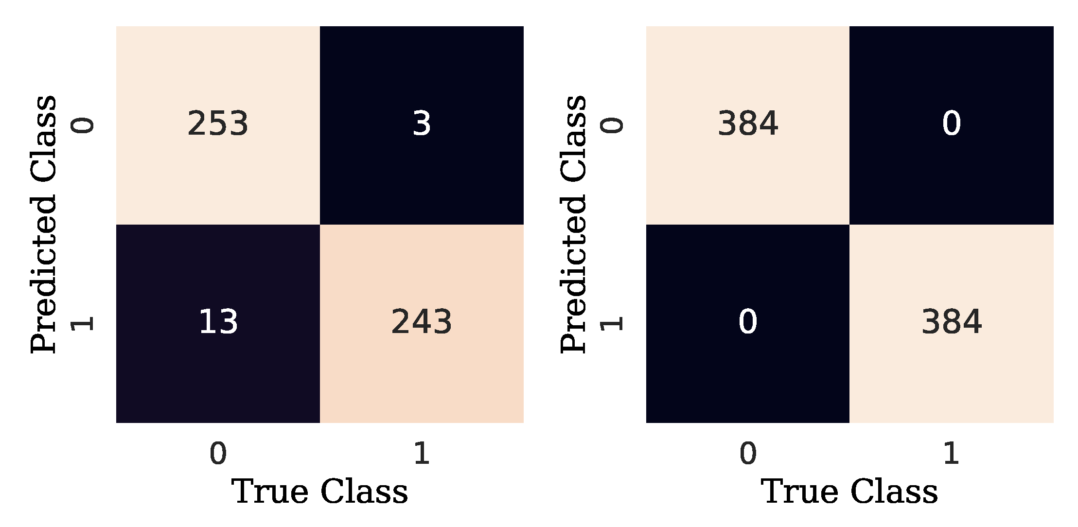
The confusion matrices obtained from the implementation of the two models, model 1 and model 2, in both stages (damage detection and damage diagnosis) are shown in
Figure 15 and
Figure 16. For the first model, the failed predictions consist of 18 FPs and 3 FNs for the detection stage, and 13 FPs and 3 FNs for the diagnosis stage. As it can be observed, adding an extra convolutional layer to the SNN feature extraction stage can improve the performance of the model in both stages, since the confusion matrices show neither FPs nor FNs.
Figure 17 and
Figure 18 demonstrate the same confusion matrices, but using a 70%, 15%, and 15% data split (for the training, validation, and testing sets, respectively). The results are shown to be comparable to those obtained with the 80%, 10%, and 10% data split.
A follow-up was conducted on the performance of model 1, according to the different levels of WN amplitude factors (0.5, 1, 2, 3) for the initial 80%, 10%, and 10% data split. The purpose was to find how many failed predictions are made for each of the different WN amplitudes.
Figure 19 (left) shows the results for the damage detection stage. Specifically, it can be seen that, for the case of WN with amplitude factor 0.5, there are no wrong predictions. Similarly, for the WN amplitude factor 1, there is only one incorrect prediction that is at least identified as belonging to amplitude 1. In the case of WN amplitude factor 2, there are seven incorrect predictions that are assigned as similar to amplitude factor 0.5. Finally, for WN with factor 3, there are 10 incorrect predictions that map to WN with factor 0.5, and two incorrect predictions where the model assimilates them to samples in WN factor 1.
Figure 19 (right) shows similar results but for the damage diagnosis stage. These results can be summarized in the following manner. When an image comes from a WT operating at higher wind speeds (simulated in the experimental tower with a higher white noise amplitude factor), the model has far more failed predictions, which is in good agreement with the insight obtained in the exploratory data analysis performed in
Section 3.2.
In
Table 9,
Table 10,
Table 11 and
Table 12, a deeper exploration of the results is shown to gain an insight on how many FP or FN outputs are obtained, according to the structural state, among the images by model 1. It is shown that the predictions given by model 1 (one convolutional layer) for both cases, damage detection and damage diagnosis, output a higher number of FNs than FPs. Furthermore, model 2 (two convolutional layers) outperformed model 1 with no false predictions.
Eventually, the accuracy, precision, recall, and F1 score for both stages and models are detailed in
Table 13 and
Table 14. The results show that the damage detection and damage diagnosis results are promising, as they achieved great performance on different structural state samples.
Finally, to thoroughly test the functional characteristics of the algorithm, a comparison is made with four other methodologies given in [
31], [
32], [
13], and [
12] that use the same laboratory structure. The first methodology, given in [
31], is based on principal component analysis and support vector machines. The second methodology, given in [
32] (page 67), is based on the well-known damage indicators: covariance matrix estimate and scalar covariance. The third methodology, given in [
13], is based on machine learning methods and the fractal dimension feature. The last methodology, given in [
12], utilizes a signal-to-image conversion of the accelerometer data into multichannel images and convolutional neural networks (CNN), combined with synthetic data augmentation. First, when using the first approach stated in [
31], the crack damaged bar has a recall of 96.08% and is therefore inferior to the one obtained with the strategy proposed in this work, which reached a value of 100%. Note that the crack damage is the most challenging. In fact, the second approach stated in [
32] (page 82) was unable to detect this type of incipient damage when using scalar covariance or mean residual damage indicators. Furthermore, the first approach obtains a recall of 99.02% for the unlocked bold damage, while, with the proposed strategy, a slightly higher value of 100% is obtained. Note that the unlocked bold damage is not studied in the second approach. The third approach [
13] requires hand-made feature extraction, and the performance metrics obtained are inferior to those obtained in the present study. Furthermore, the machine learning methods proposed in [
13] need a large data set to achieve good performance, while Siamese neural networks have the ability to learn from very little data, which is crucial in the specific application faced in this work. Finally, the fourth approach [
12] requires a deep CNN as well as a data augmentation of 25,200% in the total number of samples to achieve 99% accuracy, while, with the proposed strategy, a better accuracy is obtained using much fewer data and a much simpler neural network architecture.
5. Conclusions
In this work, the proposed test bench consists of a WN generator, connected to an amplifier that simulates different wind speed regions of the operation of the WT. Subsequently, triaxial accelerometers are connected to obtain the vibration signals. Different simulations were carried out, taking into account four types of structural states, such as the healthy bar, the replica bar, the crack damaged bar, and the unlocked bolt. It was concluded that, when wind speeds are higher (regions where turbines operate or are desired to operate most of the time), it is more challenging to distinguish when a sample belongs to a specific state. The main contribution of this work is informing the use of SNNs for the damage detection and damage diagnosis stages. Increasing the number of convolutional layers to extract features from the data increased the performance of the model. The conceived SHM methodology with two convolutional layers showed exceptional performance, demonstrating results of 100% for all considered metrics. These findings indicate that SNNs are promising for developing SHM techniques for offshore platforms.
Note that this study is a proof-of-concept contribution, as the data were obtained in a controlled laboratory environment. Therefore, as future work, it is proposed to incorporate other environmental conditions, such as the wave excitation, by placing the experiment in a water tank facility to simulate the effect of regular and irregular waves. Finally, it is important to note that environmental and operational conditions (EOC) play an important role when dealing with long-term monitoring because they can complicate damage detection. Large variations in EOCs make EOC monitoring almost as important as structural monitoring itself. Therefore, its influence should be compensated. Several methods for EOC compensation for WTs have been developed to make SHM possible. For example, in [
33], affinity propagation clustering is used to delineate data into WT groups of similar EOC. In [
34], covariance-driven stochastic subspace identification is used. Finally, in [
35,
36], fuzzy classification techniques are used for EOC compensation. However, as noted previously, this work is an experimental proof of concept, and EOC compensation is left as future work using pattern recognition techniques in a more realistic environment.


 ,
, 


