Evaluation of the Approach for the Identification of Trajectory Anomalies on CCTV Video from Road Intersections

Abstract

The approach for the detection of vehicle trajectory abnormalities on CCTV video from road intersections was proposed and evaluated. We mainly focused on the trajectory analysis method rather than objects detection and tracking. Two basic challenges have been overcome in the suggested approach—spatial perspective on the image and performance. We used trajectory approximation by polynomials as well as the Ramer-Douglas-Peucker N thinning technique to increase the performance of the trajectory comparison method. Special modification of trajectory similarity metric LCSS was suggested to consider the spatial perspective. We used clustering to discover two types of classes—with normal and abnormal trajectories. The framework, which implements the suggested approach, was developed. A series of experiments were carried out for testing the approach and defining recommendations for using different techniques in the scope of it.

1. Introduction

A growing number of roads and highways are equipped with closed-circuit television (CCTV) cameras, which has become an essential element of modern smart cities [1]. Such cameras provide vital information about the current traffic situation on the streets. They are the main source of information for many services of intelligent transport systems (ITS), including the automatic detection of traffic jams and car incidents, vehicle counting, weather condition detection, monitoring of road conditions, etc. A growing number of ITS services working with CCTV cameras raise the problem of automatic analysis of video stream data [2,3].

One of the important ITS services for modern cities is automatic detection of vehicle trajectory anomalies [4,5,6]. Such anomalies can be caused by different reasons—car accidents, reckless drivers, road obstacles, bad road conditions, etc. The information about detected anomalies in vehicle’s behavior must be considered for decision making and effective traffic management at the top level of ITS.

Effective detection of vehicle trajectory anomalies on video streams from CCTV cameras is a complex task, which involves effective object (vehicles) detection, tracking, trajectory construction, and finally separation of trajectories into reference and anomaly classes. The main challenges here are limited computational power resources and the spatial perspective of the video [5].

In the paper, we suggested and evaluated the approach for the identification of vehicle trajectory anomalies on streaming video, which works well in the case of the mentioned challenges. We focused on determining spatial trajectory anomalies and considered them as templates, of which spatial coordinates seriously differ from other trajectory templates according to the selected distance. We focused on the detection of spatial trajectory anomalies, caused by traffic accidents, unexpected obstacles on the road, inadequate driving of the vehicle, and violation of traffic rules related to changing the vehicle’s trajectory (U-turn through a double solid line, for example).

We used computer vision methods and artificial neural networks for objects detection and tracking. Then, we used machine learning methods for trajectories construction and their classification. In the paper, we paid more attention to the study of machine learning methods that work with trajectories.

To meet the considered challenges, we investigated the efficiency of different trajectory approximation methods and introduced the new trajectory comparison metric. We compared trajectory approximation by 3-, 4-, 5-degree polynomials and the Ramer-Douglas-Peucker (RDP) N thinning technique to increase the performance of the trajectory comparison method. Special modification of trajectory similarity metric LCSS was suggested to consider the spatial perspective. Hierarchical clustering technique was used to separate vehicle trajectories into reference and anomaly classes. We carried out a series of experiments to evaluate the suggested approach, selecting the best trajectory thinning/comparison methods using the developed framework.

The structure of the paper is organized as follows. In Section 2, we consider basic knowledge related to the topic of the paper. In Section 3, we consider state-of-the-art techniques related to the identification of trajectory anomalies. In Section 4, we suggest the basic concept and algorithms for the trajectory classification approach. In Section 5, we present the results of the experiments. In Section 6, we present the discussion based on experiments to select the rational way of using the approach. In Section 7, we present the conclusion and possible further directions of work to improve the results.

2. Basic Knowledge

This section is intended to give background information and introduce useful definitions and basic concepts of approaches used in the following sections. Source data and basic challenges will be discussed.

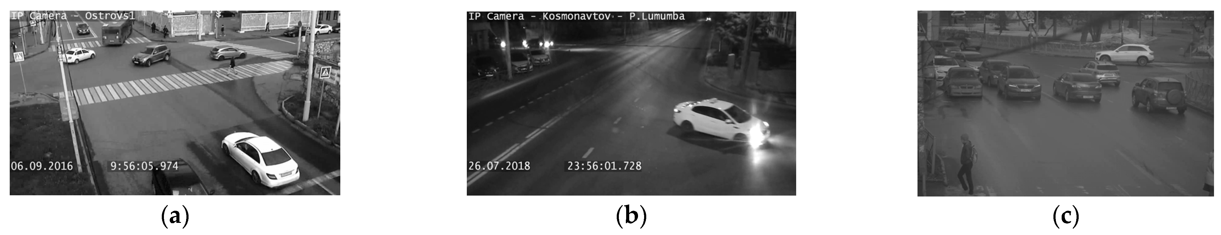
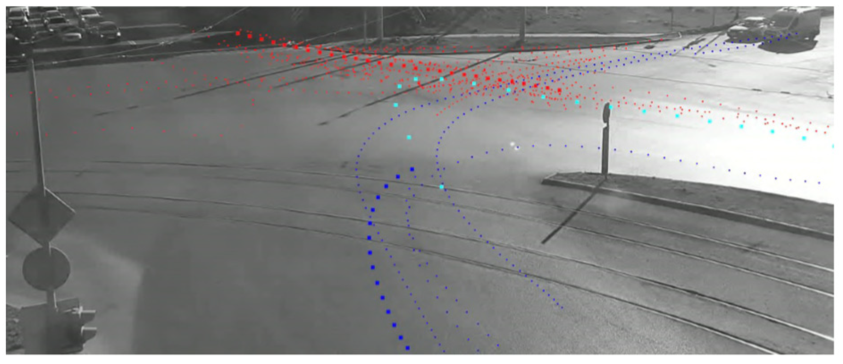
2.1. Source Data and Trajectory Definition

The main research question we considered in this paper concerns approaches and algorithms for processing trajectory data. Video data from 165 enforcement cameras, which are installed at road intersections in Kazan city, were considered as raw data (Figure 1). Video resolution is 1280 × 720, while a frame rate of 10 frames per second is used. We covered all CCTV cameras installed at road intersections in Kazan. The dataset involved 24-h recording from each camera done in one day. Following road intersection types have been included (Figure 1):

• Four-way intersections (Figure 1a);
• T-intersections (Figure 1b);
• Y-intersections (Figure 1c).

A stand-alone tracking system takes the raw video from video surveillance cameras and handles it to perform the object detection and convert the trajectory into several tracking points on images (Figure 2). The basic concept of this process is described more deeply in Section 4. The outcome of the tracking system is tracking points (TPs), containing information such as vehicle ID, timestamp, and possible spatial coordinates. These TPs are considered an input for processing in the context of the current work.

Generally, the trajectory is data which contain only minimum information, such as position and time, as well as the identifier of the tracking object. This information can be easily augmented by detailed information, such as speed, acceleration, and moving direction, since they can be extracted from the initial trajectory data [7].

We define the trajectory τ or T for the vehicle as the sequence of three-dimensional points, where the first two coordinates represent the position of the vehicle in 2D space and the third coordinate represents the time [6,8] (Formula (1)):

$$\tau =\left(x_1,y_1,t_1\right),\left(x_2,y_2,t_2\right),\dots \left(x_n,y_n,t_n\right),$$

(1)

2.2. Trajectory Anomalies

Twenty-four-hour recording video surveillance cameras produce massive amounts of data about moving objects. This fact increases the possibility that along with the normally behaving objects, some of the moving objects will demonstrate abnormal behavior. Such exceptional behaviors can also be named as outliers, anomalies, abnormalities, exceptions, novelties, or deviants [9,10].

Trajectory anomalies (outliers) could be considered as a template that seriously differs from the remaining traffic behavioral templates according to a certain metric of similarity [10]. Generally, the anomalous to normal activity patterns ratio should be relatively small to be able to distinguish abnormalities from the dominating normal patterns. According to the literature, we can divide anomalies into the following general categories [10,11,12]:

• The spatial trajectory anomaly (U-turn of a car for example);
• The temporal trajectory anomaly, detected by analyzing only temporal characteristics of trajectories, such as duration and time of moving. For example, a trajectory with a significantly long duration or a trajectory appearing at an anomalous time;
• The spatiotemporal (ST) trajectory anomaly, which can be detected by analyzing spatial and temporal information in aggregate. This type corresponds to situations where the spatial information can be considered as normal, but adding temporal information converts the trajectory into an abnormal one. Examples of ST anomalies can be vehicles moving with a considerably high or low speed compared with the majority of trajectories, and vehicles making unexpected, emergency stops. In addition, such anomalies can be detected in the case of contra-flow traffic systems with reversing traffic light anomalous trajectories: since for such line allowed direction changes according to some known or learned schedule, the classifier can analyze the trajectory direction together with temporal information.

The current work is focused on determining trajectory anomalies of the first type (spatial trajectory anomalies). In this case, we considered trajectory anomaly as a template in which spatial coordinates (x_i,y_i) seriously differ from other trajectory templates according to selected distance. In the current work, we focused on detecting the following types of spatial trajectory anomalies:

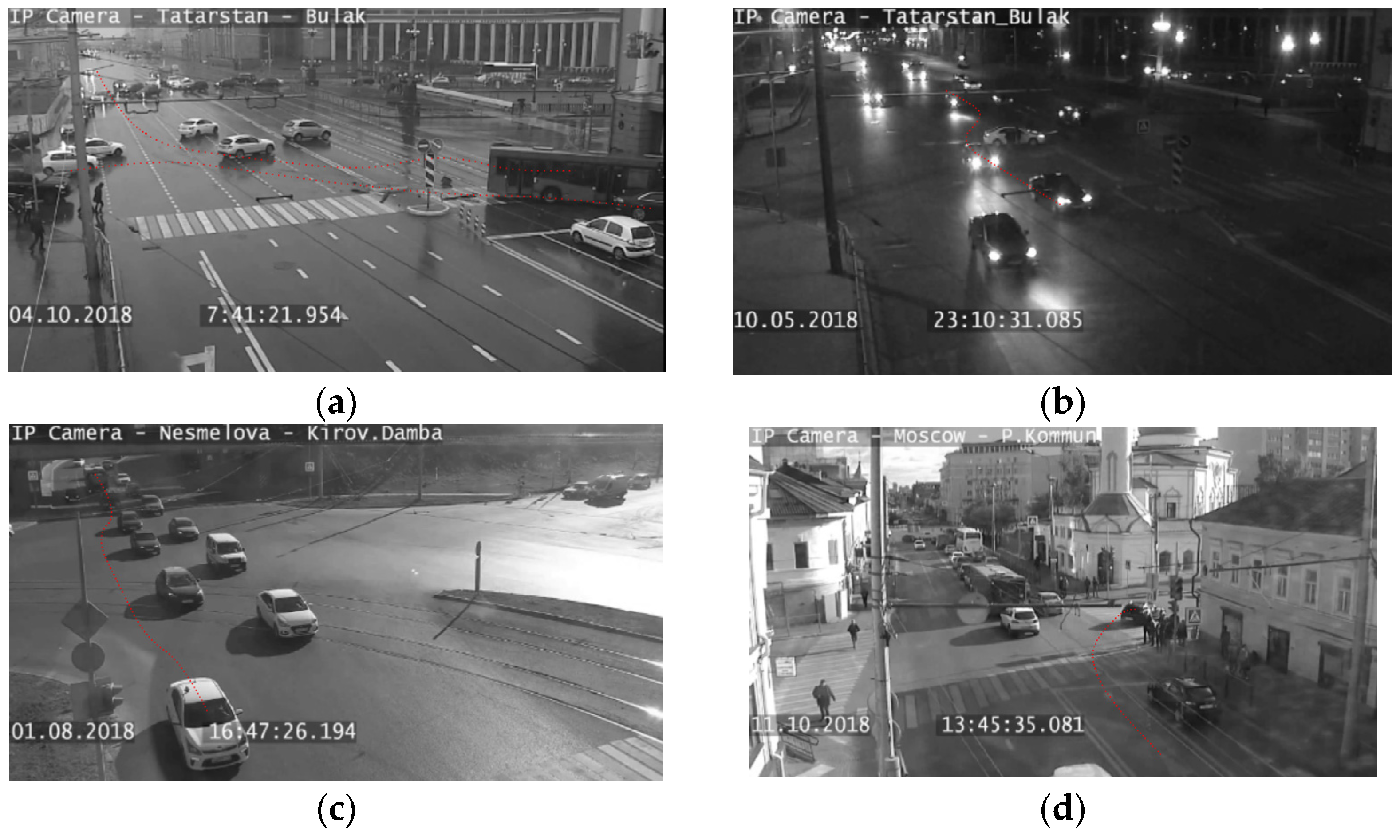
• Caused by traffic accidents, and resulting to change the vehicle’s trajectory or even in moving of vehicle into the opposite direction (Figure 3a);
• Caused by unexpected obstacles on the road (vehicle breakdown, cargo falling from the track) (Figure 3b);
• Caused by inadequate driving of the vehicle (constant lane changes, for example) (Figure 3c);
• Violation of traffic rules related to changing the vehicle’s trajectory (U-turn through a double solid line or right turn from the left line, for example) (Figure 3d).

2.3. Basic Challenges

It should be noted that the chosen type of input source leads to some challenges in their processing.

One of the basic challenges of source data is spatial perspective [12]. Video surveillance cameras are placed into the fixed locations of street intersections (Figure 2). It leads to the comparative size of detected trajectories. Trajectory points with farther dislocation from video enforcement cameras are closer concentrated than points, of which dislocation is closer. It should be considered in the definition of trajectory similarity metric.

Another important challenge for processing raw trajectories data (1) is the computing performance of algorithms. The sequence (1) often includes too many points to process. Not all of them are important for trajectory classification, but reduce the performance of the algorithms. This fact leads to the necessity of approximation or thinning of initial trajectories to leave only an important (key) point for further classification.

3. State of the Art

3.1. Trajectory Classification

There are different trajectory anomaly detection techniques described in the literature [13].

The main concept of classification-based techniques lies in using a classifier that first learns to distinguish normal and abnormal trajectories and then classifies each input instance [14]. Such techniques consist of training and testing phases. The training phase supposes learning a classifier model from a training dataset, containing labeled data instances. The learned classifier is then used to classify an input trajectory as normal or anomalous by assigning a class label in a testing phase. Some classifiers assumed that model is learned using training data containing labels for normal and anomalous classes [12]. Other classifiers assumed that training data contains only normal data instances with corresponding normal class labels [10]. A trajectory which is aligned with none of the learned normal class descriptions is considered anomalous.

Some classifiers suppose learning multiple classes during the training step and then using a classifier to review the input trajectory for compliance with each learned class.

Single-class Support Vector Machines (SVMs) is a well-known approach, which applies to the task of anomalous trajectory detection [15,16]. However, this approach requires trajectory vectors to be the same length. Since raw trajectory data usually contain different amounts of trajectory points, it is necessary to preprocess raw trajectories to normalize their length [15]. Moreover, SVMs become highly time- and memory-consuming while working with huge amounts of multi-dimensional data. The approach proposed in [15] is based on using SVM for trajectory clustering. First, all trajectories of different lengths are represented in constant-dimension space feature vectors. Then, the authors used smoothing to remove the noise, and finally, they did trajectory clustering and anomaly detection. This approach showed a 3.70% error on the synthetic dataset. In the paper [16], the authors used a mixture of Gaussian distributions model for object detection. Then, the authors used the contour tracing technique for object filtering and trajectory tracking. Next, trajectories lengths are normalized and the SVM machine learning algorithm with radial basis function kernel is used for trajectory classification. This approach demonstrated an accuracy of about 94%.

Proximity-based approaches [10,12,14] decide whether a data instance is normal or anomalous based on how close or far it is located concerning neighbors [12]. Nearest-neighbor and density-based approaches are based on the assumption that normal trajectory instances have a dense neighborhood, while anomalous instances are far from them [12]. To be able to compare the surrounding density for an instance under consideration with the density around its local neighbors, a distance (dissimilarity) or a similarity measure between two data instances needs to be specified [14]. In the case of multidimensional trajectory data, the task of distance computation becomes very expensive due to the high amount of data needed to be processed. In the paper [14], the authors suggested the approach for trajectory anomaly detection based on accumulated relative density (RLD). To reduce the trajectory feature vector size, principal component analysis was used. Then, the RLD metric based on points distribution in circles is calculated. If the point has RLD which deviates far from the mean, then it is labeled as an outlier, otherwise as normal. This approach showed a 95% detection success rate.

Clustering-based techniques aimed to group trajectories into different classes (normal and abnormal in the general case), called clusters, based on their similarity in such a way that objects in one cluster are similar to each other and dissimilar to objects in other clusters [8,17]. There are several types of clustering-based anomaly detection techniques with the following assumptions: (1) normal data instances are associated with a cluster, while anomalous data instances are not associated with any cluster, (2) normal data instances are close to the cluster center, while abnormal instances lie far away from the closest cluster center, and (3) normal data instances lie in large and dense clusters, while anomalies are associated with sparse clusters or clusters with a small cardinality [10,12]. One of the main advantages of clustering-based techniques is the ability of the majority of them to run in an unsupervised manner. In our case, the unsupervised learning methods are the most appropriate, because labeling hours of video data is a highly time-consuming task. In addition, manual labeling of input data can lead to errors due to human operator intervention. However, at the same time, these algorithms are computationally expensive.

The main concept of model-based algorithms is that they represent the data as a set of parameters to create the model of normal behavior. As an advantage, model-based approaches do not ask the user to provide any input parameters, because all the parameter values can be derived from the data. The main drawback of model-based approaches is that the data that comes from a particular distribution cannot always be satisfied, specifically in the case of multi-dimensional data [10].

In this paper, we decided to focus on clustering-based anomaly detection approaches due to the following reasons:

• They can work in an unsupervised mode without human intervention and do not require the input data to contain labels;
• Input data are allowed to contain anomalous trajectories;
• They can be easily applied to multi-dimensional data.

However, using clustering algorithms implies using similarity metrics to compare the trajectories. Thus, we have to solve the main challenges, mentioned above, with the following:

• Include a spatial perspective in the similarity metric;
• Approximation or thinning of initial trajectories to reduce the performance complexity.

3.2. Distance and Similarity Measures

Clustering-based approaches require a similarity measure to be defined between two trajectories. Distance and similarity functions can be classified as (1) working with raw representations of trajectories without any preprocessing steps and (2) working with preprocessed trajectories representations. Preprocessing can include unifying the length of trajectories or reducing the dimensionality of trajectory vectors [18]. Some of the most known and widely used traditional similarity measures are the following: Euclidean Distance, Fréchet Distance, DTW, and LCSS.

Euclidean distance between two trajectory vectors is calculated as a sum of squared differences of corresponding spatial coordinates [19]:

$$d_{ij}={\Vert T_i-T_j\Vert }_E=\sqrt{{\displaystyle {{\displaystyle \sum }}_{k=1}^m}\left({\left(t_{i_y}^k-t_{j_y}^k\right)}^2+{\left(t_{i_y}^k-t_{j_y}^k\right)}^2\right)},$$

where both trajectories consist of m tracking points and are represented by two-dimensional vectors $T_i=\left\{t_i^1,t_i^2,\dots ,t_i^m\right\}$ and $T_j=\left\{t_j^1,t_j^2,\dots ,t_j^m\right\}$. Tuples $\left(t_{i_x}^k,t_{i_y}^k\right)$ represent spatial coordinates for a k-th tracking point of i-th trajectory from a dataset. However, Euclidean distance works only with trajectories with an equal number of tracking points. Since usually vehicles move with different speeds and behavior, trajectory length is always different and that means that raw trajectories need to be preprocessed and reduced to the same size [18]. In addition, traditional Euclidean distance requires two-dimensional data, meaning that it is not able to process temporal information and is dependent on the trajectory direction: the reversed direction can cause incorrect distance measurement, which in turn leads to errors in clustering. Additionally, it fails while working with trajectories moving similarly but with different speeds and the case of different sampling rates [20].

Fréchet Distance [19] is based on Euclidean distance. It considers the positional and sequential relationship of trajectory points while calculating the similarity. The main idea of this approach is computing Euclidean distance for each pair of points from two trajectories and then designating the maximum Euclidean distance as a Fréchet Distance between them. However, since only the maximum among distance is considered, the approach is sensitive to the presence of outliers.

Dynamic Time Warping (DTW) [21,22] is one of the algorithms for measuring the similarity between two temporal time series sequences, which may vary in speed. DTW method aims to find an alignment between time-dependent sequences, such as trajectories, and can process trajectories of different lengths. According to [21], DTW distance is calculated as follows (Formula (2)):

$$D_D\left(T_i,T_j\right)=\{\begin{array}{cc}\hfill 0,& \hspace{1em}m=n=0\hfill \\ \hfill \infty ,& \hspace{1em}m=0 or n=0\hfill \\ \hfill dist\left(a_i^k,b_i^k\right)+min\{\begin{array}{c}{D}_D\left(Rest\left(T_i\right),Rest\left(T_j\right)\right)\\ D_D\left(Rest\left(T_i\right),T_j\right)\\ D_D\left(T_i,Rest\left(T_j\right)\right)\end{array},& \hspace{1em}others\hfill \end{array},$$

(2)

where $D_D\left(T_i,T_j\right)$ refers to DTW distance between two trajectory segments with lengths m and n and $dist\left(a_i,b_i\right)$ means the Euclidean Distance between two trajectory points. Function $Rest\left(T_i\right)$ takes the remaining part of a trajectory after excluding the point $a_i$. For two non-empty trajectories, the minimum distance between them is calculated recursively. Though the important advantage of the DTW method is its ability to process trajectory vectors of distinct lengths, DTW distance is not robust to noise and requires trajectory points to be continuous. Additionally, DTW distance computation is highly time-consuming and complex due to the necessity to compare distances between each pair of trajectories [23].

Longest Common SubSequence (LCSS) distance matches two trajectories based on the longest common sub-sequence between them. This metric makes some elements remain unmatched [24] and more stable to outliers in comparison with DTW [22,24]. The LCSS distance is calculated according to Formula (3) [24]:

$$D_{LCSS}\left(T_1,T_2\right)=1-\frac{LCS{S}_{\delta ,\epsilon }\left(T_1,T_2\right)}{min\left(m,n\right)},$$

(3)

where m and n are lengths of trajectories $T_1$ and $T_2$, respectively.

$LCS{S}_{\delta ,\epsilon }\left(T_1,T_2\right)$, the longest common sub-sequence between trajectories, represents the number of matched trajectory points between trajectories $T_1$ and $T_2$ and is defined by Formula (4):

$$LCS{S}_{\delta ,\epsilon }\left(T_1,T_2\right)=\{\begin{array}{cc}\hfill 0,& if m=0 or n=0\hfill \\ \hfill 1+LCS{S}_{\delta ,\epsilon }\left(Head\left(T_1,T_2\right)\right),& \left(\begin{array}{c}if\left|t_{1_{x,m}}-t_{2_{x,n}}\right|<\epsilon \\ and \left|t_{1_{y,m}}-t_{2_{y,n}}\right|<\epsilon \\ and \left|m-n\right|\le \delta \end{array}\right)\hfill \\ \hfill max\{\begin{array}{c}LCS{S}_{\delta ,\epsilon }\left(Head\left(T_1\right),T_2\right)\\ LCS{S}_{\delta ,\epsilon }\left(T_1,Head\left(T_2\right)\right)\end{array},& otherwise\hfill \end{array},$$

(4)

LCSS calculation depends on two constant parameters [18,20,24]: δ (point spacing) and ε (point distance or matching threshold):

• Parameter δ defines the maximum remoteness in terms of time (or TP indexes) between two trajectory points [24];
• Constant ε defines the size of proximity to looking for matches in terms of spatial information (X- and Y-coordinates) [24].

The Head (T) function is defined to return the first M − 1 points from the trajectory T, representing the trajectory with the last trajectory point removed. According to the implementation given in [24], the LCSS computation has a complexity of O ((m + k) δ). However, the algorithm requires a predefined constant δ and ε parameter values as an input to a method. In addition, due to the recursive way of computations, LCSS has a high computational cost [25].

The LCSS distance is the most appropriate for trajectories comparison during clustering, since it allows the trajectories to contain noise, have different lengths, object speeds and sampling rates (local time shifts in trajectories) [18]. However, this metric has to be adopted to use in trajectories clustering, to overcome the two main challenges mentioned above.

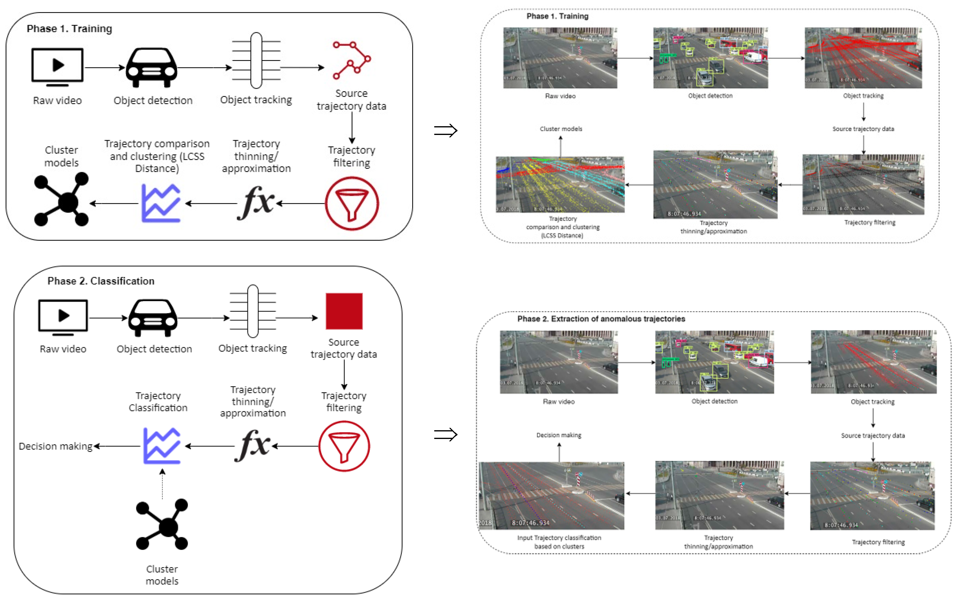
4. The Concept of Approach

The proposed approach can be described as a two-phase approach with offline clustering to extract frequent trajectories and an online classification of an input trajectory to label it as normal or anomalous.

The main workflow of the suggested approach is presented in Figure 4.

4.1. Vehicle Detection and Tracking

Our object detection and tracking algorithm follows the tracking-by-detection paradigm [26]. It implies dividing the tracking process into two stages: the detection of all objects in the frame by the detector and the linking of the corresponding detections by trackers in time to form trajectories. We used YOLOv4-tiny as an object detector. It ensures acceptable performance and a good FPS/accuracy ratio. Our tracker is based on the pyramidal implementation of the rarefied optical flow KLT. It provides reliable tracking of objects at intervals of up to five frames.

The following steps are used: detection of objects on the frame, initialization or reinitialization (updating the coordinates of an object, if it was already tracked earlier) of trackers for each found object, tracking objects on the next n frames independently. We remove objects or decide to stop tracking when objects are out of frame or disappear because of occlusion. Due to the cooperation of detector and tracker, the trajectories are collected in one piece, which gives a complete picture of the movement [27].

4.2. Trajectory Filtering

Source trajectory data in our case contain objects of different lengths and covered distances. However, due to object detection accuracy and tracker errors, some trajectories may be very small and may not look well. In contrast with the case of lost location, where the missed location can be found using approximation and regression models, the lost tracking object cannot be fixed afterward. For that reason, to improve the quality of results, it was decided to filter the input trajectories and ignore short trajectories with small covered distances. The covered distance is calculated as a Euclidean distance between the first and last TPs. We used minLength = 10 (TPs), minTotalDist = 80 (pixels) parameter values trajectories filtering. The results depicting the removed (red) and kept (black) trajectories are shown in Figure 5.

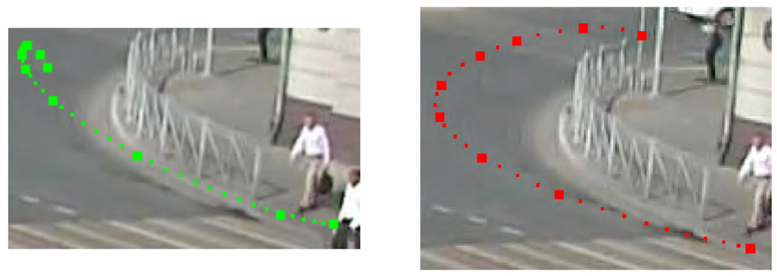
4.3. Trajectory Thinning/Approximation

As was mentioned before, notwithstanding that the LCSS similarity distance works with trajectories of arbitrary lengths and does not natively require the preprocessing of trajectories, the calculation of LCSS measure becomes extremely computationally expensive with the growth of the trajectory length because of the recursion. Moreover, most of the input trajectories contain far more TPs than needed for further analysis; this redundant information reduces the processing speed. That is why trajectory thinning/approximation is very important for further steps. It can significantly reduce the number of points in the trajectory; thus, it can significantly increase the performance of the trajectory comparison/clustering algorithms and the performance of the whole system. The main goal of this step is to leave only key points from the sequence (1), which are significant for trajectory classification.

We need to convert a given trajectory, represented by a set of TPs T = (x₁,y₁), (x₂,y₂),…, (x_n,y_n), into a subset of points T′ = (x_i1,y_i1), (x_i2,y_i2),..., (x_im,y_im), where 1 = i₁ < … < i_m = n.

We compared two methods to solve this task: (1) polynomial approximation of the sequence (1), then finding key point for approximation polynomials; (2) using Ramer-Douglas-Peucker N algorithm for thinning of the sequence (1).

4.3.1. Trajectory Approximation

We considered an approximation of points in the sequence (1) by polynomials f of some degree and find the key points where f′(τ) = 0 or f″(τ) = 0. To perform a polynomial regression the implementation provided by R. Sedgewick and K. Wayne for Java language was taken as a basis [27]. The PolynomialRegression class from Apache Commons Math 3.4.1 library takes as an input the desired degree of a polynomial (d) and two datasets of N data points consisting of real numbers: array of temporal data and an array of spatial x- or y-coordinates. Then, it performs a polynomial regression on an input set of N data points (t_i,x_i) or (t_i,y_i) and tries to fit a polynomial $x={\beta }_0+{\beta }_{1}t+{\beta }_2{t}^2+\dots {\beta }_d{t}^d$, where β_i are the regression coefficients, to minimize the sum of squared residuals of the multiple regression model. Finding the best solution for polynomial parameters is based on a Least Squares method [28].

Key points of a polynomial f(t) refer to points where the polynomial function is not differentiable or where f′(τ) = 0 or f″(τ) = 0. Such key points can denote the main turns or changes in the trajectory. The equation solvers were run on Apache Commons Math library. The derivative polynomial functions are taken from polynomials for X- and Y-coordinates. Solutions found by two solvers are merged. It was also decided to add key points calculated as border points for a trajectory by taking separately minimum and maximum X- and Y-coordinates and computing the corresponding trajectory points using a respective regression model.

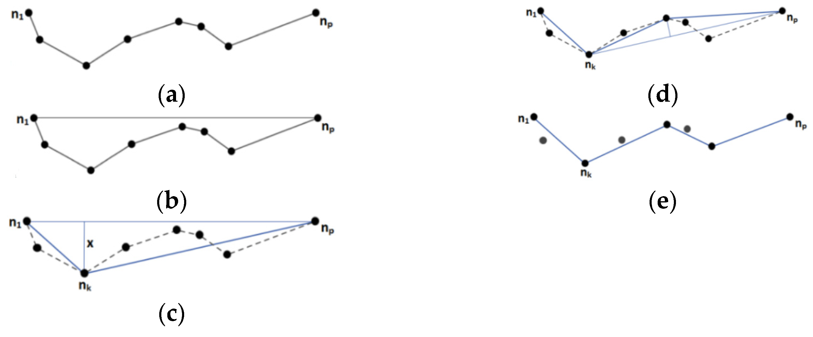
4.3.2. Ramer-Douglas-Peucker N Thinning

Another approach for solving the trajectory thinning task by reducing the number of points in a trajectory curve is Ramer-Douglas-Peucker (RDP) method. The basic idea of RDP is taking the initial trajectory and seeking another curve with a fewer number of TPs [29]. Figure 6 depicts the process of curve thinning using the RDP algorithm [30]. The method requires an initial trajectory curve consisting of an ordered set of TPs and predefined point-to-edge distance tolerance ε > 0, controlling the remoteness. The input trajectory curve is being recursively divided into segments, while the first line segment (edge) is defined by the first and last points as ends. Then, the algorithm determines the farthest point for the current line segment (line) and decides whether we need to remove or keep the point based on ε. The recursive process continues until all points from the initial curve satisfy the point-to-edge tolerance. The simplified trajectory curve can be obtained by choosing only points marked as kept. In the paper, the RDP N trajectory thinning algorithm was used to ensure the required number N of approximation points.

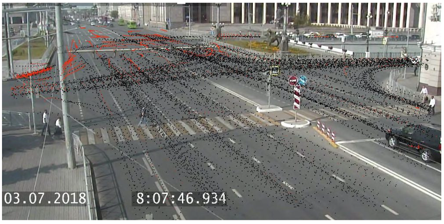
4.4. Trajectories Comparison and Clustering

4.4.1. Modified LCSS

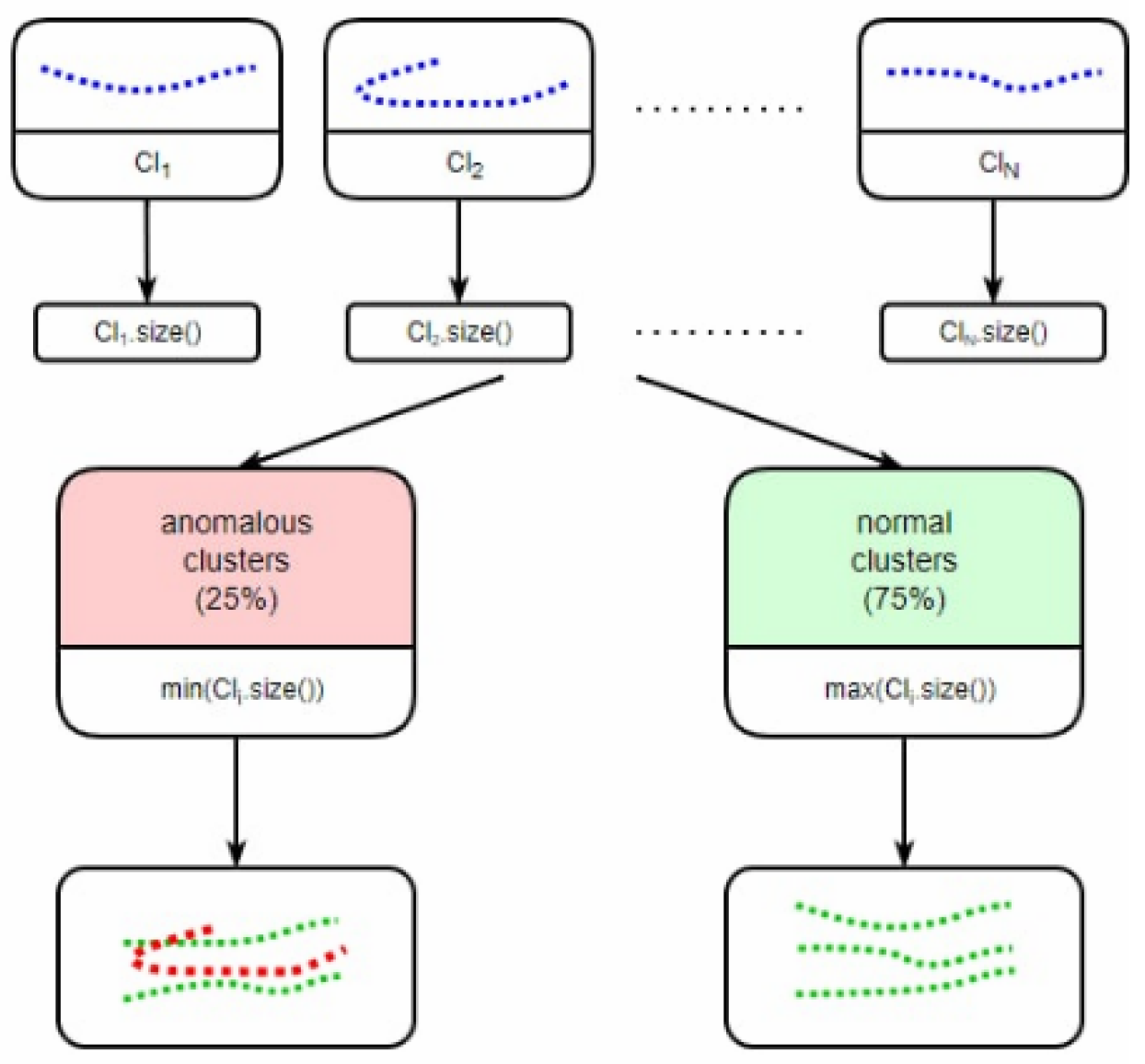
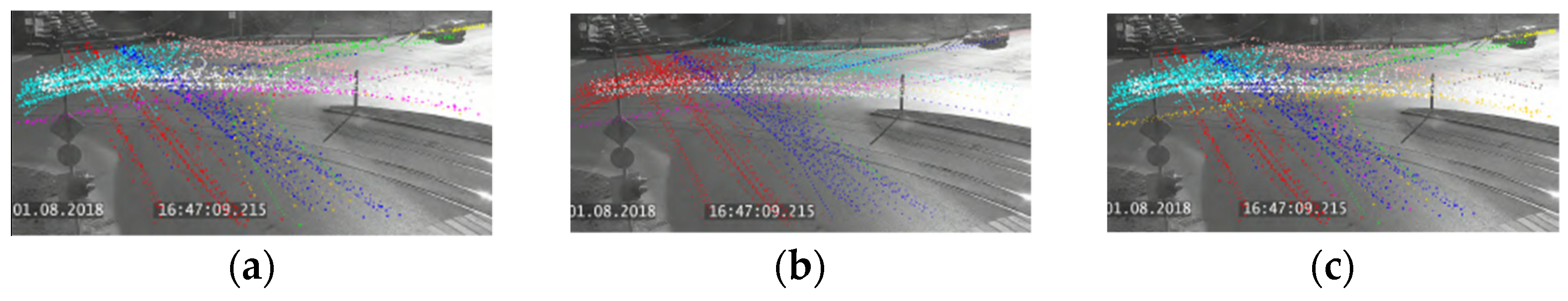
We modify the classical LCSS distance to consider spatial perspective by choosing adaptive δ and ε parameter values to work with data coming from different positions towards the CCTV camera. Value ε is the threshold controlling spatial remoteness of trajectory points while computing similarity. Consequently, it must be adapted to the remoteness and decrease as TP moves far away. We can say the same for the δ value.

In modified LCSS metric, we calculate δ and ε values in each iteration based on following formulas:

$$\delta =c_{\delta }\times minimum\left({\tau }_1·len,{\tau }_2·len\right)$$

(5)

$${\epsilon }_x=c_{\epsilon }\times \frac{\left(maxX-minX\right)}{distToCCTV}$$

(6)

$${\epsilon }_y=c_{\epsilon }\times \frac{\left(maxY-minY\right)}{distToCCTV}$$

(7)

where distToCCTV is the distance to CCTV camera from the observed point.

4.4.2. Clustering

Clustering is done in an unsupervised manner using a hierarchical clustering algorithm operating on a distance matrix between trajectories. To perform clustering, the modified LCSS distance is used as a similarity measure. The general scheme of normal and abnormal cluster construction is represented in Figure 7.

A normal cluster contains a relatively big number of trajectories. We use the concept of quantiles to distinguish clusters. In the current work, it was decided to use the 0.25-quantile (lower, first quartile) as the threshold value.

To perform a further classification of an input trajectory, we introduced a cluster model (CM)—compact definition of a cluster. We consider the cluster model as a single trajectory that is less distant from others (Figure 8).

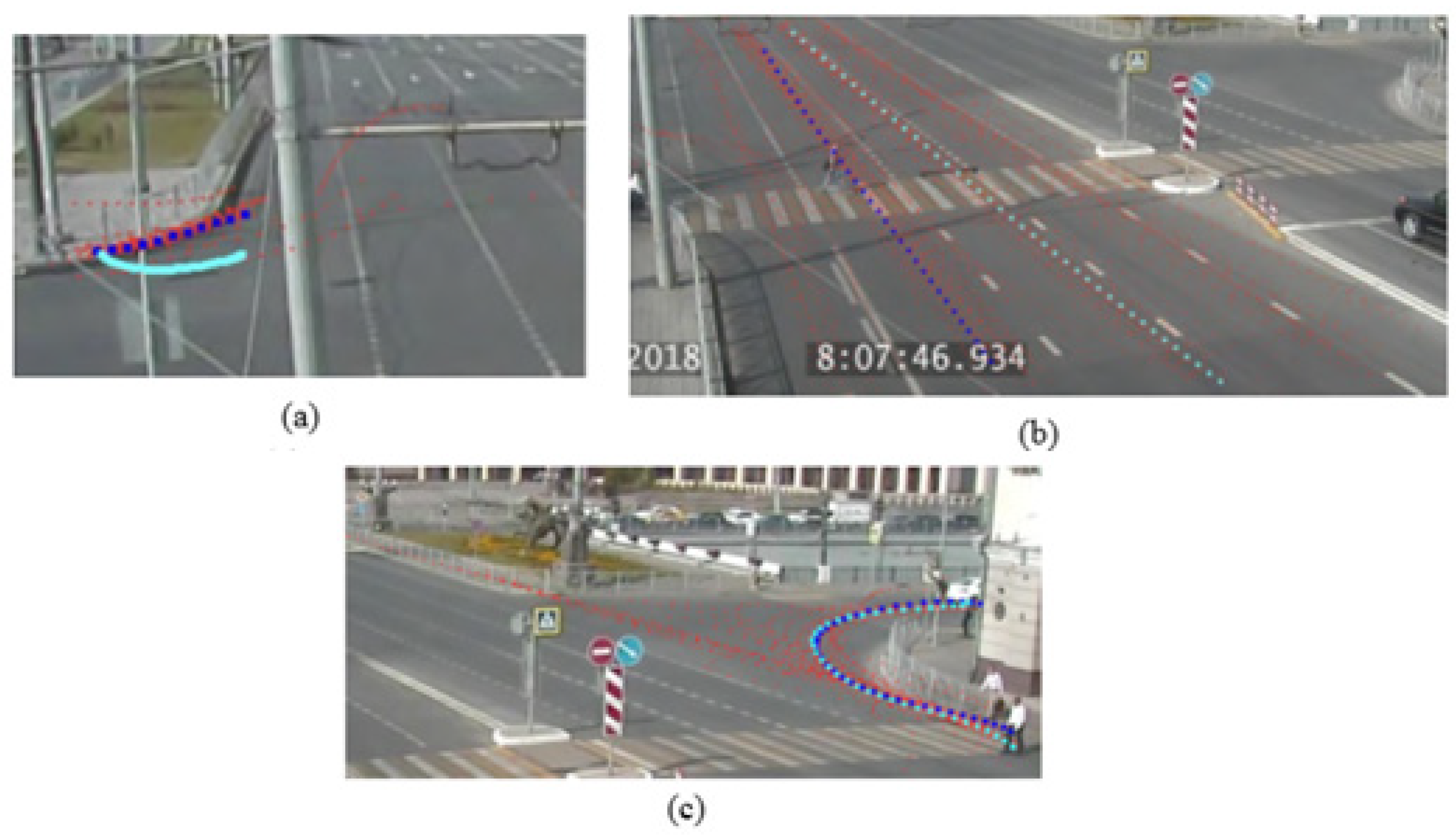
4.5. Trajectory Classification

The last step of the suggested approach is the input trajectories classification and, consequently, anomaly detection. Since the cluster models are used, classification is simplified by selecting the cluster with minimum distance to its CM. If the distance is more than some threshold, the trajectory is considered as abnormal.

5. Results

5.1. Developed Framework

To carry out the experiments with real data and evaluate suggested methods, a framework was developed. Java was used as the main programming language of the implemented framework. Commons Math library was chosen for the implementation of the approximation step. Java AWT and Swing provide a GUI to the Java application.

5.2. Evaluation of Trajectory Approximation Technique

In this section, we carried out several experiments related to trajectory approximation on the video by third, fourth, and fifth degree polynomials. Min/average R² score value was used to assess the approximation quality.

Evaluation results for the one intersection (Case 1) are presented in

Table 1. (a) Evaluation of trajectory approximation polynomials. (b) Evaluation of trajectory approximation polynomials (Cases 2–4).

Degrees of Polynomials	R2 Score
	X		Y
	Min	Avg	Min	Avg
a
Case 1 (before filtering)
{3}	0.66	0.994	0.466	0.989
{3, 4}	0.897	0.998	0.823	0.994
{3, 4, 5}	0.949	0.998	0.864	0.995
Case 1 (after filtering)
{3}	0.689	0.997	0.777	0.995
{3, 4}	0.942	0.999	0.872	0.997
{3, 4, 5}	0.98	0.999	0.88	0.997
b
Case 2 (after filtering)
{3, 4}	0.992	0.9997	0.832	0.996
Case 3 (after filtering)
{3, 4}	0.815	0.995	0.867	0.996
Case 4 (after filtering)
{3, 4}	0.879	0.995	0.722	0.993

a (before filtering and after filtering). Approximately 4.9% of the trajectories were discarded in the filtering process.

We can see that filtering out trajectories improves the results. Approximation results using third-degree polynomials are insufficient in the general case. On the other hand, approximation using third- and fourth-degree polynomials in conjunction improved both minimum and average values of R². For that reason, approximation, using several degrees, was performed with the following approach:

• Perform approximation using the lowest degree of a polynomial as a starting point;
• Compare the obtained R² with a predefined threshold; if the obtained value is less than the threshold value, increase the degree and remake the polynomial regression;
• Continue until the acceptable R² is obtained or until the limit is reached for a polynomial degree to check (5 in our case).

Evaluation results for three other intersections (Cases 2–4) were obtained according to this approach and are presented in Table 1b.

In Figure 9, we can see different trajectory approximation results with detected key points.

5.3. Evaluation of the Trajectory Thinning Technique

A comparison of the total length of approximated trajectories and the positional errors for the RDP N algorithm is represented in

Table 2. Length and positional errors for trajectories, approximated with RDP N.

Length (TPs)			Positional Error (pixels)
Min	Avg	Max (N)	Min	Avg	Max
2	6.86	7	0	12.2	432
2	7.82	8	0	9.26	388
2	8.76	9	0	7.38	340

. The minimum length is equal to 2, meaning that TPs are located on a straight line, and the trajectory coincides with the initial simplifying line, consisting of the first and last trajectory points. However, this occurs only for a small number of input trajectories. Notwithstanding that, the average length is almost equal to the desired N value. Simplified trajectories obtained by applying the RDP N (N = 9) are presented in Figure 10.

5.4. Evaluation of Trajectory Clustering Technique

We used Dunn’s Validity Index (DI) [31] to evaluate the clustering quality. In Figure 11, we can see different clustering cases using modified LCSS distance. We can see the case of using different clusters and different approximation methods.

As was described previously, clusters with small cardinalities are considered clusters of anomalous trajectories. Anomalous clusters consist of trajectories with unusual behavior. In Figure 12, we can see examples of normal and anomalous clusters. Figure 11b represents an example of anomalous clusters related to a traffic accident in source data.

5.5. Trajectory Classification

In Figure 13, we can see the results of normal trajectory classification. Red trajectories denote the closest cluster, the blue trajectory, depicted using bold TPs, emphasizes the corresponding CM, while the input trajectory is plotted using cyan color.

In Figure 14, we can see the result of anomaly trajectory classification (blue points).

5.6. Evaluation of Performance

We carried out the experiments on a PC with Intel^® Core ™ i5-3470 CPU@ 3.20 GHz (4CPUs), 8192 RAM. A video stream with 438 preliminary filtered trajectories with an average length of 29 TPs was considered.

Approximation using the Polynomial Regression method works fast and consumes only 256 milliseconds for the whole set of input trajectories, with an average consumption of ≈0.6 milliseconds per trajectory. The process of finding a polynomial function itself takes 73 milliseconds. The average length of approximated trajectories equals to 7.4 TPs.

Approximation using an RDP algorithm takes 55 milliseconds. We have got the results on trajectories with lengths within 7 and 12 TPs, with an average of 7.96 points. Approximation using an RDP N algorithm for N = 8 takes 223 milliseconds, which is less than a Polynomial Regression but longer than a traditional RDP algorithm. Approximated trajectories lengths lie within 7 and 8 TPs with an average value of 7.98 TPs before and within 5 and 8 with an average of 7.87 TPs after excluding the redundant points.

Table 3. LCSS distances calculation.

Approximation Method	Time (ms), Total	Avg Time (ms) Per Pair	Comment
438 trajectories, 95,703 trajectory pairs
Polynomial Regression	1,162,153 ms (19.37 min)	12.4 ms	Average trajectory length 7.43 TPs
Ramer-Douglas-Peucker N, N = 8	2,110,364 ms (35.2 min)	22.05 ms	Average trajectory length 7.87 TPs

presents the results of performance evaluation for LCSS Distances Calculation and using different approximation methods.

Table 4. Trajectory clustering.

Case	Time (ms), Total	Trajectory Pairs, Per ms	Comment
Case 1	1310	73	438 input trajectories, 95,703 trajectory pairs
Case 2	323	66.6	208 input trajectories, 21,528 trajectory pairs
Case 3	267	69	193 input trajectories, 18,528 trajectory pairs
Case 4	240	66.4	179 input trajectories, 15,931 trajectory pairs

presents the results of the performance evaluation for agglomerative hierarchical trajectory clustering.

5.7. Comparison with Other Methods

The suggested approach is based on unsupervised learning. Therefore, trajectories in the training dataset do not have any labels. In this case, it is hard to compare the suggested approach with supervised learning methods, presented in Section 3. However, we can compare them conceptually and highlight the following advantages:

• Manual labeling of trajectories in source data is not needed;
• It is possible to detect some new types of spatial trajectory anomalies, which have not been included in the training set.

We also carried out a series of experiments to compare the existing approach with the following methods:

• Using the DBSCAN algorithm instead of hierarchical clustering;
• Using the original LCSS distance instead of its modification suggested in Section 4.4.1.

The efficiency of using DBSCAN according to the DI index for Case 1 is presented in

Table 5. DI index for DBSCAN.

#	ε	Min Pts	Number of Clusters, DI
1	300	20	6, DI = 0.88
2	270	20	7, DI = 0.87
3	270	15	6, DI = 0.86
4	270	10	5, DI = 0.92
5	300	10	5, DI = 0.91
6	250	10	5, DI = 0.92
7	250	5	5, DI = 0.91
8	200	10	11, DI = 0.79
9	200	5	9, DI = 0.53
10	200	2	11, DI = 0.47
11	150	10	6, DI = 0.73
12	150	5	11, DI = 0.8
13	150	2	24, DI = 0.48

. We can say that the best DI value is 0.92, which is less than the value we have got with using hierarchical clustering (0.95). Moreover, the DBSCAN algorithm has to be modified to an adaptive ε value to take into account the spatial perspective.

The best DI value when using the original LCSS distance to compare the trajectories is 0.77, which is less than the value we have got with using modified LCSS (0.95).

Therefore, we can say that in both cases., the suggested method showed better efficiency.

6. Discussion

6.1. Discussion of Evaluation Results

According to the evaluation results, for the case of the polynomial regression, the best accuracy of the approximation is achieved while using the third- and fourth-degree polynomial functions jointly. In the case of using an RDP N algorithm, setting the desired trajectory length to eight trajectory points led to the best relation between the complexity of the inter-trajectory distance calculation and the necessity to keep the initial trajectory form.

Thereby, clustering was performed on a filtered set of approximated input trajectories using key points for each of them. The accuracy of the performed clustering was evaluated using a DI index and is equal to approximately 0.95, which can be considered as an acceptable result and denotes a qualitative division into clear distinguishable clusters.

As a result of this work, the following conclusions and deductions can be drawn:

• Approximation of short trajectories with a non-constant speed requires higher-order polynomial functions for approximation;
• Notwithstanding that LCSS distance allows trajectories to be of different lengths, it becomes extremely computationally expensive and complex for trajectories with more than 11–12 trajectory points;
• Approximation using a polynomial regression works well with the trajectory data, since it is known in advance that spatial coordinates of a trajectory are functionally dependent on the time;
• Approximation using an RDP N algorithm works faster and more accurately in terms of keeping the spatial information and representing main curves of the initial trajectory according to calculated positional errors, but Polynomial Regression is preferable for the cases when temporal information is needed to be preserved and analyzed;
• Using the adaptive parameter values significantly increases the accuracy of the results.

6.2. Discussion of Possible Real-World Applications

One of the major questions that has to be discussed is how ITS systems could utilize the information about detected trajectory anomalies. We discuss below possible real-world applications once trajectory anomalies are detected.

The first real-world application is the integration of the developed framework with some emergency management information systems (EMIS). One of the potential EMIS that could be used for that is GLONASS+112, which is used in Kazan city [32], as well as the CCTV cameras we used in this paper. Let us consider some scenarios associated with this integration:

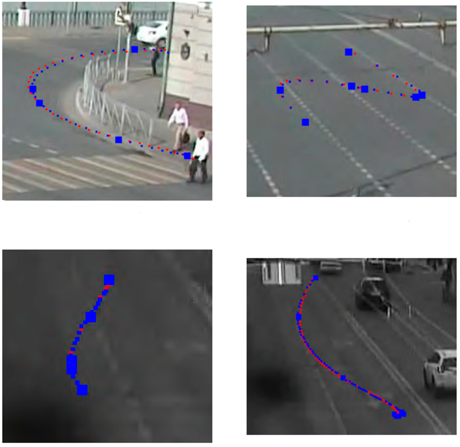
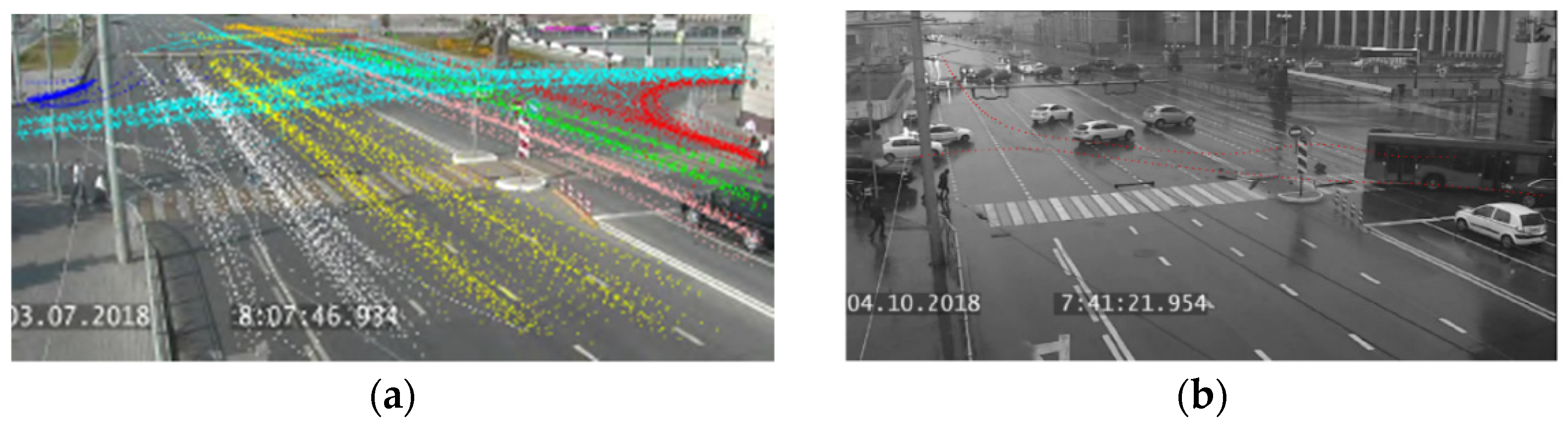
• Detection of trajectory anomalies caused by traffic accidents, and resulting, for example, in the vehicle moving into the opposite direction. A clear example of such accident is presented in Figure 12b. In this case, the ITS system can send an emergency message to EMIS GLONASS+112 for immediate response and call the necessary emergency services (ambulance, police, etc.). Such an automatic response can reduce the potential damage from emergency events and even save human lives.
• Detection of trajectory anomalies caused by unexpected obstacles on the road (vehicle breakdown, cargo falling from the track). In this case, the ITS system can send a warning message to EMIS GLONASS+112 to call the necessary road services, traffic police, etc.
• Detection of trajectory anomalies caused by inadequate driving of the vehicle (constant lane changes, for example). In this case, the ITS system can also send the warning message to EMIS GLONASS+112 to call the traffic police.

Another essential real-world application is the integration of the developed framework with car navigators. For example, information about facts, described in scenarios 1–3 could be used by car navigator applications to predict possible traffic jams and construct the best routes that eliminate road congestion.

The third important real-world application is the integration of the developed framework with variable-message signs (Figure 15). For example, information about facts, described in scenarios 1–3, could be used to inform car drivers about possible difficulties of driving in certain directions.

6.3. Some Limitations of the Approach

The suggested approach is focused on unsupervised learning (clustering). It has some advantages, as described before. First, time-consuming manual data labeling is not needed in this case. Second, it is possible to detect new types of trajectory anomalies that have not been included in the training set.

However, the suggested approach has some limitations, which have to be mentioned:

• The efficiency of the suggested approach strongly depends on the dataset with training data. This dataset should be representative, include different types of road intersections, functioning at different times of the day, with traffic jams and without them, with working traffic lights and without them. We can expect misdetections if some correct trajectory types have not been included in the training set.
• The model has to be retrained if traffic regulations change or if any long-term obstacles appear in the CCTV camera view (for example, road works are being carried out).

We considered these limitations during the model training (source data are described in Section 2.1.).

7. Conclusions

In this work, an approach for the identification of trajectory anomalies on video streams from CCTV cameras, installed on the road intersections, was suggested. This approach can be used at any intersection by the implementation of two main phases: training of the model and trajectory classification/anomaly detection. The approach has been implemented in the framework on Java language. The research was concentrated only on processing the trajectories defined by a set of points. The processing of such trajectories is complicated by two main challenges—spatial perspective and performance. Our approach can overcome these challenges by trajectory approximation and thinning, as well as key point detection. We adopted a well-known LCSS metric to work with the spatial perspective. We also used a hierarchical clustering approach to identify trajectory anomalies. The implemented algorithm is designed in an offline-learning manner, which means that models of normal trajectories are learned offline beforehand and are not updated with new upcoming data on an ongoing basis. Future research can include investigating the opportunity of updating normal trajectories database to make the framework more adaptable to actual traffic data.

References

1. Mohandu, A.; Kubendiran, M. Survey on Big Data Techniques in Intelligent Transportation System (ITS). Mater. Today Proc. 2021, 47, 8–17. [Google Scholar] [CrossRef]
2. Buch, N.; Velastin, S.A.; Orwell, J. A review of computer vision techniques for the analysis of urban traffic. IEEE Trans. Intell. Transp. Syst. 2011, 12, 920–939. [Google Scholar] [CrossRef]
3. Singh, K.; Jain, P.C. Traffic Control Enhancement with Video Camera Images Using AI. Lect. Notes Electr. Eng. 2020, 648, 137–145. [Google Scholar]
4. Mehboob, F.; Abbas, M.; Jiang, R.; Rauf, A.; Khan, S.A.; Rehman, S. Trajectory Based Vehicle Counting and Anomalous Event Visualization in Smart Cities. Clust. Comput. 2018, 21, 443–452. [Google Scholar] [CrossRef]
5. Koetsier, C.; Busch, S.; Sester, M. Trajectory Extraction for Analysis of Unsafe Driving Behaviour. ISPRS-Int. Arch. Photogramm. Remote Sens. Spat. Inf. Sci. 2019, 42, 1573–1578. [Google Scholar] [CrossRef] [Green Version]
6. Ahmed, S.A.; Dogra, D.P.; Kar, S.; Roy, P.P. Trajectory-Based Surveillance Analysis: A Survey. IEEE Trans. Circuits Syst. Video Technol. 2019, 29, 1985–1997. [Google Scholar] [CrossRef]
7. De Aquino, A.R.; Alvares, L.O.; Renso, C.; Bogorny, V. Towards semantic trajectory outlier detection. In Proceedings of the Brazilian Symposium on GeoInformatics, Campos do Jordão, SP, Brazil, 24–27 November 2013; pp. 115–126. [Google Scholar]
8. d’Acierno, A.; Saggese, A.; Vento, M. Designing Huge Repositories of Moving Vehicles Trajectories for Efficient Extraction of Semantic Data. IEEE Trans. Intell. Transp. Syst. 2015, 16, 2038–2049. [Google Scholar] [CrossRef]
9. Liu, H.; Li, X.; Li, J.; Zhang, S. Efficient Outlier Detection for High-Dimensional Data. IEEE Trans. Syst. Man Cybern. Syst. 2018, 48, 2451–2461. [Google Scholar] [CrossRef]
10. Chandola, V.; Banerjee, A.; Kumar, V. Anomaly Detection: A Survey. ACM Comput. Surv. 2009, 41, 1–58. [Google Scholar] [CrossRef]
11. Grubbs, F.E. Procedures for Detecting Outlying Observations in Samples. Technometrics 1969, 11, 1–21. [Google Scholar] [CrossRef]
12. Santhosh, K.K.; Dogra, D.P.; Roy, P.P. Anomaly Detection in Road Traffic Using Visual Surveillance: A Survey. ACM Comput. Surv. 2021, 54, 1–26. [Google Scholar] [CrossRef]
13. Malik, K.; Sadawarti, H.; Kalra, G. Comparative analysis of outlier detection techniques. Int. J. Comput. Appl. 2014, 97, 12–21. [Google Scholar] [CrossRef]
14. Liu, S.W.T.T.; Ngan, H.Y.T.; Ng, M.K.; Simske, S.J. Accumulated Relative Density Outlier Detection for Large Scale Traffic Data. Electron. Imaging 2018, 9, 1–10. [Google Scholar] [CrossRef]
15. Piciarelli, C.; Micheloni, C.; Foresti, G.L. Trajectory-Based Anomalous Event Detection. Circuits Syst. Video Technol. IEEE Trans. 2008, 18, 1544–1554. [Google Scholar] [CrossRef]
16. Batapati, P.; Tran, D.; Sheng, W.; Liu, M.; Zeng, R. Video Analysis for Traffic Anomaly Detection using Support Vector Machines. In Proceedings of the 11th World Congress on Intelligent Control and Automation (WCICA), Shenyang, China, 29 June–4 July 2014; pp. 5500–5505. [Google Scholar]
17. Nguyen, H.L.; Woon, Y.K.; Ng, W.K. A Survey on Data Stream Clustering and Classification. Knowl. Inf. Syst. 2014, 45, 535–569. [Google Scholar] [CrossRef]
18. Ghrab, N.B.; Fendri, E.; Hammami, M. Abnormal Events Detection Based on Trajectory Clustering. In Proceedings of the 13th International Conference on Computer Graphics, Imaging and Visualization (CGiV), Beni Mellal, Morocco, 29 March–1 April 2016; pp. 301–306. [Google Scholar]
19. Eiter, T.; Mannila, H. Computing Discrete Fréchet Distance. In Technical Report CD-TR 94/64; Technische Universitat Wien: Vienna, Austria, 1994. [Google Scholar]
20. Vlachos, M.; Kollios, G.; Gunopulos, D. Discovering Similar Multidimensional Trajectories. In Proceedings of the 18th International Conference on Data Engineering, San Jose, CA, USA, 26 February–1 March 2002; pp. 673–684. [Google Scholar]
21. Yuan, G.; Sun, P.; Zhao, J.; Li, D.; Wang, C. A Review of Moving Object Trajectory Clustering Algorithms. Artif. Intell. Rev. 2017, 47, 123–144. [Google Scholar] [CrossRef]
22. Toohey, K.; Duckham, M. Trajectory similarity measures. SIGSPATIAL Spec. 2015, 7, 43–50. [Google Scholar] [CrossRef]
23. Mueen, A.; Chavoshi, N.; Abu-El-Rub, N.; Hamooni, H.; Minnich, A.; MacCarthy, J. Speeding up dynamic time warping distance for sparse time series data . Knowl. Inf. Syst. 2018, 54, 237–263. [Google Scholar]
24. Toohey, K. R Package Documentation. Similarity Measures. LCSS. Available online: https://rdrr.io/cran/SimilarityMeasures/man/LCSS.html (accessed on 30 June 2021).
25. Zhang, Z.; Huang, K.; Tan, T. Comparison of similarity measures for trajectory clustering in outdoor surveillance scenes. In Proceedings of the 18th International Conference on Pattern Recognition (ICPR’06), Hong Kong, China, 20–24 August 2006; Volume 3, pp. 1135–1138. [Google Scholar]
26. Makhmutova, A.; Anikin, I.V.; Dagaeva, M. Object Tracking Method for Videomonitoring in Intelligent Transport Systems. In Proceedings of the 2020 International Russian Automation Conference, RusAutoCon, Sochi, Russia, 6–12 September 2020; pp. 535–540. [Google Scholar]
27. Sedgewick, R.; Wayne, K. Polynomial Implementation. Available online: https://algs4.cs.princeton.edu/14analysis/PolynomialRegression.java.html (accessed on 11 November 2021).
28. Hadi, I.; Sabah, M. Behavior formula extraction for object trajectory using curve fitting method. Int. J. Comput. Appl. 2014, 104, 28–37. [Google Scholar] [CrossRef]
29. Douglas, D.H.; Peucker, T.K. Algorithms for the reduction of the number of points required to represent a digitized line or its caricature. Cartogr. Int. J. Geogr. Inf. Geovisualization 1973, 10, 112–122. [Google Scholar] [CrossRef] [Green Version]
30. Mokrzycki, W. New version of Canny edge detection algorithm. In Proceedings of the International Conference on Computer Vision and Graphics (ICCVG), Warsaw, Poland, 24–26 September 2012; pp. 533–540. [Google Scholar]
31. Dunn, J.C. Well-separated clusters and optimal fuzzy partitions. J. Cybern. 1974, 4, 95–104. [Google Scholar] [CrossRef]
32. Dagaeva, M.; Garaeva, A.; Anikin, I.; Makhmutova, A.; Minnikhanov, R. Big spatio-temporal data mining for emergency management information systems. IET Intell. Transport. Syst. 2019, 13, 1649–1657. [Google Scholar] [CrossRef]
Figure 1. Road intersection types. Four-way intersections (a). T-intersections (b). Y-intersections (c).
Mathematics 10 00388 g001
Figure 2. Tracking points.
Mathematics 10 00388 g002
Figure 3. Types of spatial trajectory anomalies. (a) Traffic accident; (b) Unexpected obstacle; (c) Inadequate driving; (d) Violation of traffic rules.
Mathematics 10 00388 g003
Figure 4. The main workflow of the suggested approach.
Mathematics 10 00388 g004
Figure 5. Results of trajectories filtering.
Mathematics 10 00388 g005
Figure 6. Trajectory thinning using the RDP algorithm. (a) Initial trajectory; (b) Point-to-edge distance; (c) Separation trajectory into segments; (d) Selection points for keeping; (e) Final trajectory.
Mathematics 10 00388 g006
Figure 7. Normal and abnormal cluster construction.
Mathematics 10 00388 g007
Figure 8. Cluster model.
Mathematics 10 00388 g008
Figure 9. Trajectory approximation and key points.
Mathematics 10 00388 g009
Figure 10. Trajectory approximation using RDP N.
Mathematics 10 00388 g010
Figure 11. Clustering results (a) Polynomial regression, 11 clusters, DI = 0.94; (b) RDP N regression, N = 8, 11 clusters, DI = 0.95; (c) RDP N regression, N = 8, 9 clusters, DI = 0.93.
Mathematics 10 00388 g011
Figure 12. Examples of normal and anomalous clusters. (a) Normal clusters. (b) Anomalous clusters (traffic accident).
Mathematics 10 00388 g012
Figure 13. Results of normal trajectory classification.
Mathematics 10 00388 g013
Figure 14. Results of the anomaly trajectory classification.
Mathematics 10 00388 g014
Figure 15. Variable-message sign.
Mathematics 10 00388 g015