Gas Path Fault and Degradation Modelling in Twin-Shaft Gas Turbines


1
School of Engineering, University of Lincoln, Lincoln LN6 7TS, UK
2
Siemens Industrial Turbomachinery, Lincoln LN5 7DF, UK
*
Author to whom correspondence should be addressed.
Machines 2018, 6(4), 43; https://doi.org/10.3390/machines6040043
Submission received: 18 August 2018
/
Revised: 19 September 2018
/
Accepted: 20 September 2018
/
Published: 1 October 2018
(This article belongs to the Special Issue Fault Detection, Diagnosis, and Recovery: Concept, Modeling, and Optimization)
Abstract
:In this study, an assessment of degradation and failure modes in the gas-path components of twin-shaft industrial gas turbines (IGTs) has been carried out through a model-based analysis. Measurements from twin-shaft IGTs operated in the field and denoting reduction in engine performance attributed to compressor fouling conditions, hot-end blade turbine damage, and failure in the variable stator guide vane (VSGV) mechanism of the compressor have been considered for the analysis. The measurements were compared with simulated data from a thermodynamic model constructed in a Simulink environment, which predicts the physical parameters (pressure and temperature) across the different stations of the IGT. The model predicts engine health parameters, e.g., component efficiencies and flow capacities, which are not available in the engine field data. The results show that it is possible to simulate the change in physical parameters across the IGT during degradation and failure in the components by varying component efficiencies and flow capacities during IGT simulation. The results also demonstrate that the model can predict the measured field data attributed to failure in the gas-path components of twin-shaft IGTs. The estimated health parameters during degradation or failure in the gas-path components can assist the development of health-index prognostic methods for operational engine performance prediction.
1. Introduction
Industrial gas turbines (IGTs) are widely used to generate electricity or drive rotating machinery such as pumps and process compressors. Performance of gas turbine engines gradually deteriorates over the service life due to degradation of the gas-path components such as the compressor, the combustor, and the turbines.
These physical faults gradually evolve over a prolonged period of operation and lead to degradation of the individual gas-path components. Engine performance is represented by a set of so-called health parameters such as efficiency and flow capacity of individual components. These health parameters deviate from initially healthy baseline values as the engine components degrade. Estimation of health parameters from engine data is often referred to as gas path analysis [1,2]. Weighted-least-square estimation [3,4] and Kalman Filters [5,6,7] are widely used for gas path analysis (GPA). More recently various techniques such as neural networks [8,9,10], Bayesian belief networks [11], genetic algorithms [12], polynomial functions [13], and different hybrid methods [14,15] have been explored for use in performance fault diagnosis and tracking.
Recent studies on diagnostic and prognostics techniques to predict maintenance and optimise gas turbine operation have been reported in the literature. A survey about condition monitoring as well as diagnostic and prognostic techniques using performance parameters acquired from gas-path data has been carried out by Hanachi et al. [16]. The review discusses the advantages and limitations of the diagnostic and prognostic techniques commonly used for gas turbines. The review suggests some considerations for constructing modern diagnostics and prognostics frameworks such as: physics-based modelling based on non-linear and dynamic gas-path models, the use of hybrid techniques for diagnostic results during instantaneous measurements, and global pattern recognition to consider failure events from across the fleets of similar gas turbines. Kang and Kim [17] developed a model-based gas turbine diagnostic method using a compressor map adaptation. The method was applied to measurement data from a 150 MW class gas turbine. It can determine whether or not the measured point corresponds to a full-load operation. When the measured point does not correspond to full-load operation, the method can predict the measurement at full-load operation. The results demonstrated that not all measured points with the full inlet guide vane (IGV) open corresponded to a full-load operation. It was also possible to predict a reduction in power output due to compressor fouling conditions. A review of the performance-based health monitoring as well as the diagnostics and prognostics of gas turbines has been carried out by Tahan et al. [18]. The review discusses five areas to consider for health monitoring in gas turbine maintenance such as performance degradation and gas path analysis, performance adaptation and simulation, techniques for fault detection and isolation, principles of fault identification, and prognostic enhancement in health monitoring. The review emphasises the importance of the development of condition monitoring systems based on transient data that can capture the fast-nonlinear dynamics of the engine. An advanced performance adaptation system to estimate the steady state performance of gas turbine models at off-design conditions is presented by Tsoutsanis et al. [19]. The method consists of a novel method for compressor map generation and a genetic algorithm to match gas path measurements of an engine at off-design conditions. The method can generate compressor and turbine maps of an engine model from real-world engine data. This can assist the development of model-based gas path diagnostics and prognostics applications.
Engine models can be used in gas turbine diagnostics. They can be used to determine performance baseline in order to calculate differences between measurements and such a baseline. They can be also used to obtain fault signatures, which represent different engine faults and degradation mechanisms. In addition, they can play an important role to predict the performance of an engine at different operating and ambient conditions and allow the estimation of parameters that cannot be measured where instrumentation is not accessible for engines operated in the field. The use of adaptative models has been demonstrated to be a powerful method for diagnosing failures in gas turbine components [20,21]. The method requires measured quantities to estimate parameter characteristics related to the performance of components (maps). Deviation between the value from a reference map and a value on the actual map can provide information component deterioration. The condition of components in a gas turbine using the adaptative model method has been reported by Mathioudakis et al. [22]. The analysis demonstrated that it can successfully identify mechanisms such as turbine blade deposits and compressor fouling which affect the performance of gas turbines. A diagnostic method based on a zooming approach and an engine adaptive model to evaluate compressor performance was reported by Aretakis et al. [23]. Component zooming consists of higher analysis code to provide higher simulation accuracy for engine diagnostics. The integrated formulation provided a reliable fault identification capability for the assessment of compressor performance.
Simulink environment is a powerful programming environment for modelling, simulating, and analyzing multidomain dynamical systems such as gas turbines. Several studies have reported gas turbine models developed in a Simulink environment. A derivative-driven diagnostic pattern analysis method to predict the dynamic performance of gas turbines has been reported by Tsoutsanis and Meskin [24]. A window-based prognostic method is implemented with an engine gas turbine model constructed in Matlab/Simulink. The method is tested through the simulated parameters from an engine model representing multiple component degradations. The compressor degradation can be predicted through a local linear window-based approach. The method has demonstrated that gas turbine component degradation for engines under transient operation can be accurately predicted. An engine model developed in a Matlab/Simulink environment to predict the transient response of an aeroderivative engine for mechanical drive and power generation applications has been reported by Tsoutsanis et al. [25]. The model considers mass momentum and energy balance equations and can be adapted to any kind of gas turbine configuration. It can be applied for real-time model-based diagnostics and prognostics technologies. A recent study reported by Tsoutsanis et al. [26] proposed component map modelling methods implemented in their previously Matlab/Simulink gas turbine model [25] to predict the set of equations for replicating the compressor and the turbine map data in gas turbines. The developed method could assist any condition monitoring and health estimation strategy to improve operation and define maintenance strategies for gas turbines. A Simulink model of a gas turbine engine developed from a Fortran model to simulate fault data and to train neural networks for fault diagnosis is reported by Patel et al. [27]. The model considers different features of a gas turbine engine such as nonlinearities, fast changing dynamics, continuous and discrete parameters, multiple sample rates, and multiple inputs and outputs. Fault data were generated by the Simulink model to train neural networks for fault diagnosis. In the authors’ previous study [28], a Simulink gas turbine model of a twin-shaft IGT was developed using a commercial thermodynamic library compatible with the Simulink environment. The developed model demonstrated that it has the potential to assist the development of a diagnostic tool using a neural network for compressor fouling during IGT operation.
A Simulink model to predict the transient response of an industrial power plant gas turbine (IPGT) was reported by Asgari et al. [29]. The Simulink Model was constructed from thermodynamic and energy equations. The simulated data from the Simulink Model were compared with the predicted data from a nonlinear autoregressive exogenous (NARX) model. The results showed that both Simulink and NARX models successfully provided satisfactory prediction of the dynamic behavior of the gas turbine. Watanabe et al. [30] reported a dynamic model developed in Matlab/Simulink to analyze the dynamical behavior of industrial power systems with a customer’s gas turbine power plant. A GUI with object-oriented configuration allowed a friendly application of the model for the analysis of industrial power systems. The static characteristics predicted by the model were consistent with experimental measurements.
Yu et al. [31] reported a modular non-linear gas-turbine digital-control system constructed in a Simulink environment. The volume-inertia method was considered to construct a three-shaft gas-turbine in Simulink. The simulated data were compared with measurements from gas turbine manufacturers. The results showed that the digital-control system model can predict real gas turbine measurements. Gobran [32] reported a Simulink model to calculate the off-design running point for single shaft Centaur 40 power generation gas turbine. The effect of ambient conditions on temperature and pressure across the gas turbine at the design condition was discussed. The simulated data predicted by the model were compared with field data. The model did not consider compressor and turbine characteristic maps, and scaling factors were considered to adapt the characteristics of the simulated engine. The results demonstrated that the Simulink model can predict the field data of the engine. Srikanth et al. [33] developed a Simulink model of a single shaft microturbine generator (MTG) connected to distribution networks (grid connection and islanding operation). The authors also described the different control strategies for MTG with grid connection and islanding operation. The results showed that it is possible to simulate the power flow in both the directions between grid and MTG.
The aforementioned Simulink models only simulate engine performance at optimal conditions (no failure in components). In this study, degradation and fault modes on for the gas-path components of a twin-shaft IGT have been considered for discussion and demonstration of gas path model-based diagnostic methodology. The non-linear gas turbine model developed in a Simulink environment can predict the performance of a twin-shaft IGT at different ambient and operating conditions. The developed Simulink architecture allows the introduction of empirical parameters to simulate failure and degradation modes in gas-path components and overall performance reduction in engine. The contribution of the proposed Gas Path Fault and Degradation Modelling methods includes the following:
- A modelling architecture was developed to simulate and analyze different degradation/fault modes in gas-path components of gas turbines with different dynamic degradation rates.
- As suggested in a recent literature review of diagnostics and prognostics for condition-based maintenance of gas turbines [18], it is required to develop condition monitoring systems which can capture the fast-nonlinear dynamics of the engine. The developed modelling architecture in this study can reproduce fast-nonlinear dynamics in the engine and can also estimate the dynamic change in health indices attributed to different dynamic degradation rates. This can establish a good quality data set for diagnostic and prognostic purposes.
- Prediction, analysis, and isolation of overlapping effects/failure in different engine components were carried out through a validated modelling architecture. This has a great advantage over the conventional data-based analysis, e.g., neural networks.
- The model has been validated with real measured engine data featuring failure/degradation in components at defined operating/ambient conditions. The off-design performance maps implemented in the modelling architecture could allow the simulation and prediction of the same failure/degradation mode at different operating/ambient conditions. This could be important for the planification of different maintenance strategies based on health indices for engines operated in different ambient conditions.
- The simulation of engine performance and prediction of health indices based on flow capacities and efficiencies in components in the Simulink environment could allow for the improvement of control strategies through real-time simulation and testing of embedded system to minimise the impact of failure components on the overall engine performance.
The analysis has been divided in three sections in which each section describes a different fault/degradation mode: fouling in the compressor, hot-end blade damage in the gas generator turbine (GGT), and variable stator guide vanes (VSGVs) offsetting in the compressor. A brief description of the modelling architecture of a twin-shaft engine is discussed before the three main sections describing the fault modes are presented. Each fault mode section consists of a brief literature review about mechanisms causing degradation and failure in components during engine operation. In addition, each fault mode section considers measured gas turbine data denoting reduction in engine performance. The analysis in each section is carried out by comparing measured field data with simulated data predicted by the IGT Simulink model. In addition, the change in physical parameters across the different stations of the engine during degradation and fault in the gas path components is discussed. Finally, a discussion summarising the three fault modes is presented.
2. Gas Turbine Modelling Architecture
It is possible to construct thermodynamic models of IGTs by considering available thermodynamic toolboxes or libraries compatible with a Simulink environment [34]. The IGT model, constructed as a specialised Simulink library, reported by Panov [35] is considered for the analysis and simulation of the IGT system during failure in the gas-path components. It is also possible to represent mathematical equations in the Simulink environment through defined blocks from the Simulink library. These blocks can represent mathematical operators and constants. The different modules defined in the Simulink environment and representing the different components of a twin-shaft IGT considers thermodynamic mathematical equations defined through blocks from the Simulink library, as shown in Figure 1. The Simulink model simulates the performance of a twin-shaft IGT at optimal conditions (no degradation in components). Nevertheless, it is possible to introduce empirical parameters inside the Simulink modelling architecture to simulate failure and degradation in gas-path components and overall performance reduction in engine.
Air at ambient conditions enters the compressor, and fuel in a liquid or gas state or both states is mixed together with the compressed air leaving the compressor. The burning of the air–fuel mixture through the combustor produces hot gases that expand across the turbine stages to produce power and drive the compressor through a mechanical system (bearing-shaft). Component maps for each module were implemented in the Simulink modelling architecture. Modelling assumptions have been considered to simplify the overall modelling architecture. The Simulink model considers only dry ambient conditions. No emissions such as oxides of nitrogen (NOx), carbon monoxide (CO), or unburned hydrocarbons (UHC) resulting from the fuel-air combustion are considered.
The engine components comprising the gas turbine model have been divided into two groups: the gas generator path and the power turbine path. The gas generator consists of the compressor, combustor, GGT or Compressor-Turbine, and shaft connecting compressor and GGT and involves the thermodynamic process starting from the air intake by the compressor to the hot gas entering the GGT, as shown in Figure 2. Power turbine path components consist of the low-pressure turbine, interduct, load, and mechanical shaft connecting the power turbine and load. As inputs, the model requires the load and the ambient conditions (temperature and pressure) for the air entering the compressor. The component models include the conservation of mechanical energy for engine shafts, heat-soaking effects for metal parts, and the conservation of thermodynamic energy within different gas volumes in the engine. Each of the gas streams linking the gas path components represents a vector of gas properties. Component models calculate values for their output stream elements based on their current state and values in the input stream. Each gas stream has four elements: total pressure, temperature, density, and mass flow. A gas volume with inlet and outlet flows, heat transfer to adjacent metal structure, mechanical work, and energy dissipation through component losses are features of all gas path engine components. The detailed dynamics model of gas turbine engine can be expressed with a system of non-linear differential equations and has been reported by Panov [35].
The detailed dynamics model of gas turbine engine can be expressed with a system of non-linear differential equations in state space:
where x is state coordinate vector, u is control vector, and v is vector of operating conditions. Vector ym contains measurable observable parameters, and vector yn non-measurable parameters.
To model the dynamic behavior of the individual engine component, the following generic equations for pressure and temperature were used:
where ςj and ξl are the internal thermodynamic state and mechanical variables used to model irreversible or dissipative processes. The first term in the above equations represents volume gas dynamics using an ordinary differential equation, and the second term describes the behaviour of components using nonlinear algebraic equations, which are based on steady state component characteristics.
As a gas turbine engine undergoes internal changes, these changes may be manifested in performance degradation. To account for this degradation, the original state and output equations could be augmented with an additional state vector h containing health parameters:
The vector h contains health parameters that indicate the engine health conditions. Health parameters are usually represented by efficiencies and flow capacities of the engine components. As they deviate from their normal health conditions, the performance delivered by each component degrades, and this can be recognised as a shift in component characteristics.
The amount of fuel injected into the combustor is regulated through a gas turbine controller. The gas turbine controller takes the rotational speeds and other engine measurements, such as pressure and temperature measurements at different engine stations as input signals. The controller model has been implemented with fuel flow demand and variable guide vane demand logic. A more detailed description of the sub-modules consisting of the control logic can be found in the study of Panov [35].
The analysis requires simulation of the wide time frame during degradation and failure in gas-path components. The time frame for the failure to evolve can range from minutes to hours (e.g., hot-end GGT analysis and failure in a VSGV system) and can range from days to months (e.g., compressor fouling). Model-based diagnostics employs engine models tuned to match the observed engine state in the same manner as model-based performance tracking [36]. The developed model-based diagnostic approach is based on the measurable gas turbine parameters (pressure and temperature), which have been used to estimate engine health parameters, i.e., efficiencies and flow capacities for different gas-path components. The compressor flow discharge and compressor efficiency are not measured during engine operation. These parameters can be estimated using available computational methods such as computational fluid dynamics (CFD) and through individual component testing (e.g., variation in flow in the compressor through modification of its exit area). The flow discharge and efficiency for the compressor and turbines have been estimated at optimal conditions (no failure in component) and are represented through performance maps in the Simulink engine model architecture shown in Figure 1. The deviations between efficiencies and flow capacities from optimal (no failure) conditions can be used to generate health indices and the best signature match to identify likely component degradation modes and faults in gas-path components. The deviation of flow and efficiency to generate health indices is carried out inside the Simulink model architecture by considering empirical factors that match simulated parameters with real engine measured parameters.
A number of causes can result in gas turbine performance deterioration. The aim of this model-based diagnostics is to attempt to detect one or more of these causes that are responsible for the deterioration of engine performance. Usually this detection process is based on monitoring of so-called “health indices.” Health indices are a means of determining the deteriorated component characteristics. They represent the percentage change in component characteristics usually due to component faults or gradual degradation. Typically, two health indices can be defined for any component and they correspond to the flow capacity and efficiency. The simulation of failure of the gas-path components is achieved through a modification of the values of the flow capacity and efficiency defined in the Simulink model architecture and during engine performance simulation.
3. Degradation and Fault Modes on Gas Path Components
Three degradation and fault modes for different gas path components of a twin-shaft IGT have been considered for the analysis through the model-based diagnostics approach. The IGT Simulink model shown in Figure 1 simulates the performance of a twin-shaft IGT at optimal conditions (new and clean components). Therefore, it will be required to select and vary key parameters calculated from the Simulink model such as efficiency and flow capacity from individual gas-path components to change the measurable engine parameters (temperature, pressure, rotational speed, and fuel flow rate) during failure in gas-path components. Measured field data of a twin-shaft IGT denoting reduction in performance attributed to three different degradation/failure mechanisms in compressors and GGT have been considered for the analysis. A comparison between measured field data and simulated data from the model is carried out for each fault mode. The Simulink model can predict parameters such as flow and efficiency in components—parameters that are not available or recorded in the measured field data. These parameters are considered as health engine indicators and allow the assessment of engine performance during the evolution of degradation and failure in components.
3.1. Fouling in Compressor
Fouling on the compressor reduces the performance of the engine and is present in all open cycle gas turbines [37]. A fouling condition in axial compressors is attributed to airborne particles (dust, mineral particles, etc.) attached to the blades as shown in Figure 3, which decreases the performance of the IGT. These particles can increase the surface roughness of the blades and change the angle of the air velocity passing through the blades in the axial compressor [38]. These particles can be removed by direct washing of the compressor blades.
Humidity of air during fouling conditions can also lead to short-term compressor performance deterioration, as a lower amount of condensed water droplets may increase the amount of deposit formation on the blades [39]. It has been reported that optimum humidity condensation in the air can remove airborne particles from the compressor blades [40]. Several studies have proposed different techniques to investigate the effect of fouling conditions on compressor performance [41,42,43,44,45]. Hanachi et al. [46] developed a logarithmic regression model and an adaptive network-based fuzzy inference system ANFIS-based prediction model to estimate the future fouling state in gas turbine compressors. The ANFIS model considered the rate of humidity condensation in the compressor and allowed a better performance prediction of short-term fouling state in gas turbine compressors. Aker and Saravanamutto [47] reported a linear fouling model to simulate the progressive build-up of contaminants in the compressor by modifying the appropriate stage flow and efficiency characteristics in a stepwise fashion. It is known that the discharged air flow and discharged air pressure as well as isentropic efficiency in the compressor decrease during fouling conditions. Tarabrin et al. [48] developed a mathematical model of a progressive compressor fouling using the stage-by-stage method. The analysis was carried out in a compressor GTE-150 LMZ. The authors reported a reduction in air flow by 4.5%, pressure ratio by 4%, and efficiency by 2%. During fouling conditions, an increase in fuel is required to compensate for the loss of generated power during engine operation at low operating point. However, during high power engine operation, fuel demand is limited by the maximum turbine inlet temperature. Therefore, the change in compressor discharge temperature at fouling conditions will depend on the power engine operation.
The performance of a twin-shaft IGT at fouling conditions will be predicted using the Simulink model shown in Figure 1. It is possible to estimate the change or reduction of air flow discharged by the compressor and compressor efficiency during fouling conditions.
3.1.1. Measurements during Fouling Conditions
Measurements from a twin-shaft IGT operating as a mechanical drive at low-power condition and operating as a power generator at high-power condition were considered for the analysis. The measurement tools consist in physical sensors across the different stations from the engine, such as temperature, pressure, and rotational speed. The engine was continuously operated at steady-state during low- and high-power conditions and from a clean compressor condition to a highly fouled condition. In the first case, the engine was operated at 60% of the maximum rated power (low power condition) and in the other case the engine was operated at 90% of the maximum rated power (high power condition). Figure 4 shows the measured power output during fouling conditions when the engine is operated as a mechanical driver (low power) and as a power generator (high power). The engine operated as a power generator was continuously operated from compressor clean conditions to fouled conditions for approximately 1152 h. The engine, as a mechanical driver, was operated for approximately 1944 h from a compressor clean condition to a fouled condition. The power output was reduced during high power operation from 90 to 82% of the maximum rated power. When the engine was operated at lower power and as a mechanical driver, the power output was reduced from 60 to 55%. The decrease in power output during engine high power operation can be attributed not only to compressor fouling condition but also to the fact that, under the high-power operating condition, the maximum GGT inlet temperature limits the fuel demand. This action is carried out by the controller in which the amount of fuel is regulated to not exceed the maximum GGT inlet temperature during engine operation. Hence, a decrease in power output is expected. This effect will be discussed in more detail in the next section, accounting for fault in the GGT. It seems that the reduction in power during high power operation could be attributed to the compressor fouling condition and the increase in GGT inlet temperature. The compressor flow air and the compressor efficiency are not available in the measured field data. These parameters can be estimated through the Simulink model and play an important role as indicators of engine performance health during compressor fouling.
3.1.2. Parameter Estimation for Fouling Condition Analysis
The modelling architecture shown in Figure 1 for the simulation of engine performance at compressor fouling conditions requires the measured power shown in Figure 4 as an input. The oscillations of the measured power shown in Figure 4 can be related to the noise during the data acquisition process. A polynomial curve has been fitted to the measured power using the Curve Fitting Toolbox from Matlab software. The resulting fitted curve has been considered as input in the Simulink modelling architecture. This is important to only predict the dynamic change in the measured data during compressor fouling conditions and to isolate the noise attributed to the instrumentation and data acquisition process. The compressor module requires a map that correlates rotational speed, pressure ratio, mass flow rate, and efficiency. The compressor performance map considered in the gas turbine model represents optimal (clean) conditions. The compressor module requires as inputs the rotational speed and the pressure ratio in order to calculate air flow rate and, depending on the efficiency defined in the map, calculates the discharge temperature. Song et al. [38] demonstrated that it is possible to create a compressor performance map at fouling conditions by using analytical relations (velocity triangles) for axial compressors. This study does not consider a fouled compressor map for the analysis; therefore, an empirical analysis, which considers coefficients to reduce air flow discharged by compressor and compressor efficiency, was carried out. Empirical coefficients to reduce air flow and compressor efficiency were introduced in the compressor module from the Simulink model to predict the reduction in performance of the IGT at fouling conditions.
The compressor module defined in the Simulink environment considers compressor efficiency and capacity maps defined through blocks from the Simulink library. The nondimensional coefficients were implemented in the Simulink environment using a constant block and a product block. A constant block together with a product block modify the value of the flow capacity and efficiency, which in turn modify the thermodynamic properties such as pressure and temperature calculated by the thermodynamic equations defined in the compressor module, as shown in Figure 5. A detailed description of the model consisting of the compressor module can be found in the study reported by Panov [35].
The compressor module shown in Figure 1 does not predict values for air mass flow and efficiencies at fouling conditions. The empirical analysis allowed the prediction of the performance of the IGT at compressor fouling conditions. The coefficients were estimated by selecting different measurements along the full range of measurements during gas turbine operation in the field as a power generator and as a mechanical driver, respectively. The coefficients that allow reduction in performance of the IGT were estimated through a parameter tuning method using the Simulink Design Optimisation Toolbox [49]. The toolbox allows the optimisation of physical system parameters to meet time-domain and frequency-domain requirements and increase model accuracy. It formulates parameter estimation as an optimisation problem. The optimisation-problem solution is the estimated parameter values. A sequence of steps is required during the optimisation or estimation of the parameters. These steps consider data preparation, definition of parameters to estimate, optimisation algorithm (nonlinear least squares), and the validation of the measured data with the simulated model response considering the estimated parameters. Different iterations for the parameter estimation are carried out until a minimum error between measured data and simulated data from the model is present.
To predict the performance of the IGT at fouling conditions, the air flow and compressor efficiency calculated from the compressor map at clean conditions are multiplied by the estimated coefficients. Air flow and compressor efficiency predicted by the compressor module are not constant during IGT system simulation at fouling conditions. Variation in these values is dependent on the level of fouling, operating/ambient conditions, and corresponding gas turbine governing.
3.1.3. Comparison between Measured and Simulated Data during Compressor Fouling
The measured and simulated data have been normalised with respect to measurements at clean and optimal conditions (Hour 0). Figure 6 shows measured and simulated pressures discharged by the compressor during fouling conditions when the engine is operated as a power generation unit (Figure 6a) and as a mechanical drive unit (Figure 6b). The results show that the Simulink model can predict the decrease in compressor discharge pressure during fouling conditions. The compressor discharge pressure is reduced by 5% from clean conditions (Hour 0) to high fouling conditions (1152 h) when the engine is operated as a power generator, as shown in Figure 6a. For the case when the engine is operated as a mechanical driver, the compressor discharge pressure is reduced by 3% at high fouling conditions (1944 h), as shown in Figure 6b. During IGT operation at fouling conditions, the pressure discharged by the compressor is reduced [48].
Figure 7 shows the measured and simulated compressor discharge temperatures during fouling conditions. As discussed in Section 3.1, the change in temperature discharged by the compressor will depend on the operating condition of the engine. Figure 7a represents the compressor discharge temperature for the case as a power generation unit. Figure 7b represents the compressor discharge temperature when the engine is operated as a mechanical drive unit. When the engine was operated as a power generation unit, the compressor discharge temperature did not show a continuous increase with time. This is due to the fact that the gas turbine was intermittently limited on GGT inlet temperature. When the engine is operated as a mechanical driver, the compressor discharge temperature is increased by 3.8% from clean (Hour 0) to high fouling conditions (1944 h). The case presenting a higher level of fouling for the engine operated as a power generator and as a mechanical driver can be identified through the estimation of compressor discharge air flow and efficiency.
Figure 6 and Figure 7 relate to measurements in the gas generator-path during compressor fouling conditions. It is required to compare simulated data with measurements from the power turbine-path of the twin-shaft IGT as well, as the reduction in compressor performance during fouling conditions has an adverse effect on both gas generator and power turbine components. Figure 8 shows the simulated and measured interduct pressure. The pressure of the fluid passing across the interduct connecting the GGT and power turbine is reduced during compressor fouling conditions. A higher reduction in interduct pressure and compressor discharge pressure is observed during high power operation (power generator), as shown in Figure 6a and Figure 8a, compared to the case at low power operation (mechanical driver), as shown in Figure 6b and Figure 8b.
Simulated and measured data for the exhaust temperature leaving the power turbine are shown in Figure 9. The power turbine exhaust temperature is increased during compressor fouling conditions. The power turbine exhaust temperature is increased by 1% for the case when the engine is operated as a power generator. For the case when the engine is operated as a mechanical driver, the power turbine exhaust temperature is increased by 6%. The small increase in power turbine exhaust temperature for the power generator case could be attributed to the fact that the engine was operated for 1152 h, compared to 1944 h for the mechanical driver case, but other factors such as emissions or unburned hydrocarbons resulting from the fuel-air combustion could also be attributed. During high power operation, GGT maximum inlet temperature limits the performance of the engine. This action is carried out by the controller in which it reduces the amount of fuel demanded in order to maintain the GGT inlet temperature up to its maximum allowed value. When the GGT inlet temperature increases, a reduction in fuel yields a reduction in power output, as shown in Figure 4. When the engine is operated at partial load as in the case of the mechanical driver, the increase in temperature during fouling conditions does not increase GGT inlet temperature up to its maximum allowed value.
3.1.4. Compressor Health Parameters during Fouling Conditions
As previously mentioned in Section 3.1.2, the oscillation in the measured data can be attributed to noise during the data acquisition process and instrumentation (sensors). A polynomial curve has been fitted to the measured power and used as an input in the Simulink model to predict only the dynamic change in the measured data during compressor fouling conditions. Polynomial curves have also been fitted into the measurements such as pressure and temperature across the IGT using the Curve Fitting Toolbox from Matlab software. Figure 10 shows the measured, fitted, and simulated pressures in the interduct connecting the GGT and the power turbine.
The absolute value of the percentage error between the simulated and fitted curve for pressure and temperature across the different stations of the twin-shaft IGT was calculated. Table 1 shows the error between simulated and fitted curve for the case when the engine is operated at high power and as a power generation unit. It shows that the maximum error is at 1.23% for interduct pressure. The interduct component aerodynamically connects the gas generator turbine with the power turbine. The absolute value of the percentage error between the simulated and measured data was calculated as well as shown in Table 2. The Simulink model can predict the trend of measurements with accuracy when the engine is operated at high power as a power generation unit. Table 3 shows the error between simulated and fitted curves for the case when the engine is operated at low power and as a mechanical drive unit. The error between simulated and measured data for the case when the engine is operated at low power and as a mechanical drive unit is shown in Table 4. The maximum error is presented for the power turbine exhaust temperature at high fouling conditions and increases with increasing fouling conditions. The combustor efficiency decreases when the engine is operated at low power compared to high power operation. The error between measured and simulated power turbine exhaust temperatures could be attributed to an inaccurate estimation of the combustor efficiency as the composition of the fuel/air mix changes with increasing fouling condition during low power operation. This will be addressed in future work.
Figure 11 shows the estimated reduction of compressor discharge air flow and reduction of compressor efficiency during fouling conditions. The data have been normalised with respect to data at clean and optimal conditions (Hour 0). The compressor discharge air flow and compressor efficiency are not available in the engine measurements.
In Figure 11, it can be noticed that there is a lower compressor discharge air flow rate (a reduction of 2.59% with respect to optimal conditions) for the case at high power (power generator) and at high fouling conditions (1152 h). The compressor discharge air flow estimated when the engine is operated at low power and as a mechanical driver is reduced by 1.69% at high fouling conditions (1944 h). The flow and pressure are parameters are directly correlated; as the flow decreases, the pressure decreases, and vice versa. The high reduction in compressor discharge air flow at fouling conditions for the power generator case yielded a high reduction in pressure across the twin-shaft ITG, as demonstrated in Figure 6a and Figure 8a. It is possible to state that the case when the engine is operated at high power and as a power generator presents a higher level of fouling compared to the case for the engine operated at low power and as a mechanical driver.
In addition, different points across the range of measured field data from Hour 0 to the last hour of measured data were selected to demonstrate the reduction of flow and efficiency during fouling conditions, as shown in Figure 12. The Simulink model allows the simulation of the dynamic change in air flow and efficiency during the full range of engine operation from clean to fouling conditions. This could assist in the development of prognostic algorithms to predict the evolution of IGT performance at fouling conditions during a longer period (e.g., 6 months) when measurements are not available.
3.2. Hot-End Blade Damage in Gas Generator Turbine
The GGT, also known as the compressor-turbine, drives the compressor in a twin-shaft IGT arrangement. During high power engine operation, the GGT inlet temperature limits the power output of the gas turbine. Typically, cooling on the trailing edge of the turbine blades is usually difficult to achieve; therefore, during high temperature operation, structural damage (typically oxidation) in this section of the blade can arise. In addition, the fact that the trailing edge of the turbine blades is thin by design, the high temperature of the fluid leaving the combustor may have a propensity to deteriorate the finer features of the blade at a disproportional rate. In addition, degradation or oxidation of the turbine material may emanate due to internal object damage (IOD) events that may be attributable to high temperature turbine operation as shown in Figure 13. If a hot-end damage condition is present in the turbine, the flow capacity increases, and the efficiency decreases. According to Razak [50], the change in engine performance during a hot-end damage incident is mainly attributed to a reduction in the turbine efficiency.
Some studies have been focused on the evaluation of failure in gas turbine blades. Zhou et al. [51] proposed a physical-based damage evaluation model for high temperature blades of gas turbines. The model can predict the thermodynamic performance, mechanical stress, and creep damage of the blades in gas turbines. The results show that it is possible to evaluate the online life of a turbine blade during high temperature operation. The model could also be a valuable tool for the reliability of gas turbines. Carter [52] reported the common failures in gas turbines blades. The mechanisms that affect turbine blades such as mechanical damage through either creep or fatigue and high temperature corrosion (or oxidation) are discussed. Mishra et al. [53] analysed the failure of an un-cooled turbine blade in an aero gas turbine engine. The results showed that thermal cracks due to surface oxidation were found to be the cause of the blade failure. In addition, malfunction of sensors in the engine control system during high temperature operation was found responsible for initiating the thermal cracks. Kolagar et al. [54] investigated a first stage turbine blade failure in a 6.5 MW gas turbine. Several experimental methodologies were applied to identify potential failure reasons such as visual examination, fractography, and microstructural characterisation used by optical and scanning electron microscopes (SEM) and energy dispersive X-ray (EDX). The authors concluded that overheating was the main reason for blade failure. The mechanisms attributed to high temperature and low temperature hot corrosion in gas turbine components are discussed by Eliaz et al. [55]. High-temperature hot corrosion is attributed to the condensation of fused alkali metal salts on the surface of the component. Low-temperature hot corrosion results from the formation of Na2SO4 and CoSO4 with low melting temperatures. The authors concluded that the ultimate failure of turbine blades can result from the combination of hot corrosion and other failure mechanisms (e.g., fatigue). Overall, the studies reported in the literature argue that factors like overheating and corrosion are parameters that may lead to blade failure. In this section, the change in the physical parameters measured across a twin-shaft IGT during an IOD incident in the GGT is estimated though the IGT Simulink model described in Section 2.
3.2.1. Measurements during Hot-End GGT Damage
Measured field data such as pressure, temperature, and speed from a twin-shaft IGT operated during high power operation and as a power generator are considered for the analysis of the damage in the GGT. Under high power operating condition, the GGT inlet temperature limits the generated power output. Hot-end damage incidents may be attributed to dimensional changes of the turbine components or as a consequence IOD events. The evidence that the data considered in this analysis correspond to a twin-shaft IGT with GGT damage was corroborated after inspection. Four sets of measured data have been considered from the total range of measured data as hot-end damage incidents were present in the selected range of data. An incident from the measured data has been related to the reduction in engine performance from an initial steady-state condition to the steady-state condition resulting from a GGT hot-end damage condition. A GGT hot-end damage incident was selected from each set of measured data. Each GGT damage incident has been named as Incidents 1, 2, 3, and 4, where Incident 1 corresponds to the earliest GGT damage condition and Incident 4 is the latest GGT damage condition. The four incidents represent the same defect but at different damage conditions in which the turbine is degraded with time. An example of GGT damage incidents (Incidents 1 and 4) is shown in Figure 14, Figure 15 and Figure 16. The decrease in the measured power output as well as the estimated GGT inlet temperature allowed the identification of GGT hot-end damage incidents in the measured data. Figure 14 shows the reduction in generated power during the first and last GGT damage incident. The measured data have been normalised with respect to the measured power at optimal condition (no GGT damage) and before the reduction in power for Incident 1 at t = 0. The measured power for Incident 4 at t = 0 is less than the power measured for Incident 1 at t = 0. This difference in measured power (100%) and (95%) for Incidents 1 and 4, respectively, at t = 0 can be attributed to degradation of the GGT (material consumption) with time as two incidents (Incidents 2 and 3) were previously present.
Figure 15 shows the profile of GGT inlet temperature during Incidents 1 and 4. The GGT inlet temperature is an estimated parameter that considers measured temperatures across the compressor and interduct. During a hot-end damage incident, the GGT inlet temperature should increase, but it does not exceed a maximum allowed value. This action is carried out by the controller in which the amount of fuel is regulated to not exceed the maximum GGT inlet temperature during engine operation. The GGT inlet temperature remains constant during Incidents 1 and 4 as shown in Figure 15 because it has the maximum value when the engine is operated at high power operating conditions.
An increase in fuel demand should compensate for the loss in power output; however, under the high-power engine operation conditions, the maximum GGT inlet temperature limits the fuel demand. The performance of the engine at high operating power is limited by the GGT maximum inlet temperature. Figure 16 shows a decrease in fuel demand during the GGT damage-incident as the calculated temperature of the fluids entering the GGT as shown in Figure 15 remains at the maximum value. The fuel demand shown in Figure 16 is directly proportional to the power output shown in Figure 14. The reduction in power and fuel during Incident 4 is less than the reduction in power and fuel during Incident 1. The reduction in fuel during a GGT damage incident maintains the maximum allowed GGT inlet temperature during engine operation. As the blade material is consumed after each GGT hot-end damage incident, a faster heat dissipation in the turbine’s material is expected after each incident. Therefore, a lower reduction in fuel is required to maintain the GGT inlet temperature limit. Nevertheless, the reduction in material density in the GGT yields a reduction in engine power output during steady-state conditions.
3.2.2. Parameter Estimation for Hot-End Damage Analysis
A curve has been fitted to the measured power using the Curve Fitting Toolbox from Matlab software. The resulting fitted curve has been considered as input in the Simulink modelling architecture. Performance maps representing no failure (new & clean) conditions in the components of the IGT have been implemented in the Simulink model shown in Figure 1. The GGT map requires as inputs the rotational gas generator speed (GGS) and the pressure ratio in order to calculate air flow rate, and depending on the efficiency defined in the map, calculates the discharge temperature. To estimate the performance of the twin-shaft IGT during GGT hot-end damage conditions, nondimensional coefficients have been implemented in the GGT module from the Simulink model to predict the change in flow capacity and efficiency in the GGT. The nondimensional coefficients have been implemented in the GGT module in a similar way as implemented in the compressor module described in previous Section 3.1.2, as the compressor and GGT modules present the same modelling structure as shown in Figure 5 and Figure 17. A detailed description of the compressor model consisting of the GGT module can be found in the study reported by Panov [35].
In addition, the toolbox Simulink Design Optimisation toolbox [49] available in a Simulink environment allowed the estimation of the nondimensional coefficients to predict the flow capacity and efficiency in the GGT during a hot-end damage incident. The use of the toolbox has already been discussed in Section 3.1.2 to estimate the nondimensional coefficients that simulate a reduction in IGT performance during compressor fouling conditions.
The optimisation of the nondimensional coefficients in the GGT using Simulink Design Optimisation toolbox was carried out in two steps. First, the measured data at steady conditions and pre-damage conditions were considered; thereafter, the measured data attributed to GGT damage at steady-state conditions were considered. These resulted in two different values of the nondimensional coefficients for pre-damage and GGT damage conditions, respectively. An interpolation of the resulting values of the nondimensional parameters to account for the dynamic transition from pre-damage to GGT damage conditions was carried out. The IGT Simulink model within the nondimensional coefficients implemented into the GGT module can predict pressure and temperature measurements across the different modules of the twin-shaft IGT during a GGT damage incident.
The compressor model assumes only standard VSGV position. VSGVs ensure correct air diffusion through the compressor, and their position is controlled through a mechanism. The VSGV mechanism will be discussed in the next section, accounting for VSGV failure. The angular position of IGV is considered as a reference to change the position of the different VSGVs in the compressor through a linear motion mechanism. Actual IGV position depends on GGS and can differ for rising and falling speeds. Therefore, depending on the actual IGV position, implementing a parameter correction in the compressor module is required to account for IGV offset from the nominal schedule. If required, and depending on measured data, a nondimensional coefficient in the compressor module to account for IGV offset should be considered in the same way as the estimation of the nondimensional coefficients for the GGT using the Simulink Design Optimisation toolbox from Simulink.
3.2.3. Comparison between Measured and Simulated Data during Hot-End Damage Incidents
The analysis and prediction of the flow capacity and efficiency of the GGT through the Simulink model described in Section 2 considers the measured data related to the four incidents. Comparison between simulated and measured data has been carried out for the four incidents, but only the two extreme cases (Incidents 1 and 4) are shown for a better appreciation of the simulation results. Nevertheless, the analysis and prediction of the flow capacity and efficiency of the GGT for the four incidents are shown in the next section, as the trend for the change in flow capacity and efficiency can be related to irreversible degradation mechanisms. This will be discussed in the next section.
A comparison between measured and simulated physical parameters across the different modules of the twin-shaft IGT during a hot-end damage incident on the GGT has been carried out. The first and last measured GGT damage incidents previously mentioned in Section 3.2.1 have been considered to validate the Simulink model. Figure 18 shows the measured and simulated data for the GGS. The measured and simulated data have been normalised considering the measured data at t = 0. It is expected that a reduction in efficiency in the GGT during a hot-end damage incident yields a reduction in the GGS, as shown in Figure 18. This reduction of GGS is followed with a VSGV position that corresponds to the falling IGV schedule.
As previously mentioned, during a GGT damage incident, the IGV position could differ from a nominal schedule, which assumes a rising GGS, as shown in Figure 19. A decrease in GGS should yield a decrease in compressor discharge temperature. However, as a result of the IGV hysteresis effect where VSGVs follow a schedule of falling GGS, it is assumed that the compressor efficiency is reduced, leading to a rise in the specific power of the compressor and an increase in the compressor exit temperature. The effect of IGV offset on compressor performance will be discussed and demonstrated in detail in the in the next section describing failure in the VSGV mechanism. A non-dimensional coefficient to reduce the efficiency and hence increase the compressor discharge temperature has been implemented in the compressor module from Simulink, as shown in Figure 20 and was estimated using the Simulink Design Optimisation toolbox from Simulink [49].
Figure 18, Figure 21, Figure 22, Figure 23 and Figure 24 show the measured and simulated data for the GGS, compressor discharge temperature and pressure, interduct pressure, and exhaust temperature during the first and last incident. Figure 18, Figure 21, Figure 22, Figure 23 and Figure 24 demonstrate that the engine was operated at high operating power at steady state conditions; thereafter, a dynamic transition attributed to a GGT damage condition was present until again the steady-state condition was reached. The results show that the model can predict the physical parameters across the IGT during steady-state conditions. The change in pressure and temperature is less substantial during Incident 4 than it is during Incident 1. There is a lower reduction in power output during Incident 4 compared to Incident 1, as shown in Figure 14. This change in power output is consistent with the change in pressure and temperature for Incidents 1 and 4, respectively. The dynamic transition for power output, fuel demand, pressure, and temperature across the IGT modules is less substantial during Incidents 4 and 1. As previously mentioned, this reduction in transient response during Incident 4 could be attributed to a faster heat dissipation through the GGT blade material to maintain the maximum allowed GGT inlet temperature as material is consumed after each incident.
The reduced GGS in Figure 18 causes the compressor discharge pressure to drop correspondingly, as correctly depicted in Figure 22. However, the reduction in compressor efficiency, owing to the IGV hysteresis effect, has a much more overriding effect on the compressor exit temperature than the temperature drop that should accompany the reduced GGS and compressor discharge pressure. The pressure across the IGT is reduced during a GGT damage incident. Figure 22 shows a decrease in compressor discharge pressure during a hot-end damage incident. During a GGT damage incident, there is an increase in flow capacity discharged by the GGT. The increase in GGT flow capacity leads to a variation in compressor pressure ratio with compressor rotational speed. Therefore, a reduction in compressor discharge pressure during a GGT damage incident is expected, as shown in Figure 22.
Figure 23 shows a decrease in interduct pressure during Incidents 1 and 4. The interduct pressure is directly proportional to the compressor discharge pressure shown in Figure 22. A discrepancy between measured and simulated interduct pressures during transient conditions is shown in Figure 23. This discrepancy can be related to the fact that the dynamic variation in the nondimensional coefficients that change the flow and efficiency in the GGT during a GGT damage incident is not properly modelled. This will be addressed in the future by considering a physics-based model and the change in GGT geometry during hot-end damage. Nevertheless, it is possible to predict the steady-state variation in the physical parameters across the IGT during a hot-end damage incident in the GGT.
In addition, the model could not properly capture the dynamic transition for the exhaust temperature of the hot fluids leaving the power turbine during the GGT hot-end damage incident, as shown in Figure 24. It seems that the change in flow and efficiency in the GGT has a greater impact on the dynamic variation in the physical parameters across the modules at the back end of the engine (power path). This dynamic transition will be captured in future work and will help to enhance the control strategy of engines during a hot-end GGT damage incident.
3.2.4. Health Parameters during Hot-End GGT Damage
Polynomial curves were fitted into the measurements to analytically validate the simulation results. The mean absolute percentage error between fitted curve and simulated data at steady-state for pressure and temperature across the different stations of the twin-shaft IGT for the four hot-end GGT damage incidents has been calculated as shown in Table 5. The mean absolute percentage error between measured and simulated data has been calculated as well (Table 6). Figure 25 shows the measured, fitted, and simulated compressor discharge temperatures for Incident 1. The maximum error is presented for the interduct pressure as shown in Table 5 and Table 6. The error is calculated considering only steady-state conditions.
The change in flow capacity and efficiency in the GGT attributed to a hot-end damage incident is calculated using the Simulink model. These parameters are not available in the engine field data. The flow capacity is calculated as follows:
where is the mass flow rate discharged by the GGT, T is the temperature entering the GGT, and p is the pressure entering the GGT.
During a GGT damage incident, there is a decrease in power output and a decrease in the fuel supplied to the combustor, as shown in Figure 14 and Figure 16. The decrease in fuel is related to an increase in GGT inlet temperature during a GGT damage incident. The GGT inlet temperature limits the power output. There is an increase in the flow capacity during a GGT damage incident. The reduction in the turbine efficiency has a negative impact on the IGT performance. The calculated delta increases in flow capacity and delta reduction of efficiency for the four GGT damage incidents are shown in Figure 26. The calculated delta reductions in power output and fuel demand for the four GGT damage incidents are shown in Figure 27. The % variation (Delta) of the parameters for each incident is calculated considering initial and post-damage conditions at steady-state. Incident 1 presents a higher absolute value for % Delta Power output than the other three GGT Damage incidents, as shown in Figure 27. The absolute value for % Delta Capacity and % Delta Efficiency is proportional to the absolute value for % Delta Power output.
The power output at steady-state conditions just before Incident 3 decreased by 2.84% with respect to the power output at conditions just before Incident 1. The power output at conditions before Incident 4 decreased by 3.06% with respect to the power output at conditions before Incident 1. This reduction in power output at different GGT conditions as the engine continues operating after each GGT damage incident can be related to irreversible degradation mechanisms. Incident 4 shown in Figure 27 presents the minimum absolute value for Delta Power output.
The reason that Case 4 presents a minimum % Delta Power with respect to the other cases is attributed to the reduction in power output after each incident. The reduction in power output can be related to degradation in the GGT material. The absolute value of % Delta Fuel demand during the GGT hot-end damage condition reduced from Incident 1 to Incident 4 as shown in Figure 27. This effect can also be related to degradation or consumption of the turbine material during IOD events.
3.3. Fault in the Variable Guide Vane Mechanism of Axial Compressor
Multi-stage axial compressors consist of a number of stages. Each stage consists in a row of rotor blades followed by a row of stator blades. The kinetic energy of air is increased by the rotor blades and the stator blades transform the kinetic energy of air into static pressure. A variation in stator vane angles across the different stages of an axial compressor ensures correct air diffusion and satisfactory and safe operation of the compressor, particularly at low speeds [50]. Figure 28 shows a simplified mechanism to change the angle of the VSGVs using a single actuator. The angular position of the IGV at the front-end of the compressor is considered as a reference to change the angle of the VSGVs through a linear motion mechanism. At high engine operation speed, it is required to open the VSGVs to allow high air diffusion through the stages and avoid a compressor stall condition at the back stages in the multi-stage axial compressor.
A fault in the VSGV mechanism will change the measured IGV angle and will also change the VSGV angles across the stages of the axial compressor, as shown in Figure 29. Studies in the literature have developed compressor-stage models to predict the effect of the IGV position or change in compressor geometry on compressor performance. Song et al. [56] developed a numerical method to analyze the performance of a multi-stage axial compressor. The method considered the variation in the IGV and VSGV in the compressor performance. The results showed that the closure of vane angles yields a reduction in air flow and pressure ratio. Muir et al. [57] developed a stage-stacking method to estimate the variable geometry effects across the different stages of an axial compressor. The results showed that, by increasing in one degree the variable geometry position (closure of VSGV), there is 3% reduction in air flow, 4% reduction in fuel flow and a power loss of 5%. Failures in the VSGV system of a multi-stage axial compressor of an IGT were investigated by Tsalavoutas et al. [58]. The results showed that VSGV faults decrease the engine load and fuel flow for a given controller setpoint. In addition, VSGV faults of the first stages have a greater impact on engine performance. In this study, the Simulink model described in Section 2 is considered for the analysis of the performance of a twin-shaft IGT during fault in the VSGV mechanism.
3.3.1. Measurements during Failure in VSGV Mechanism
Measured field data from a twin-shaft IGT denoting fault in the mechanism that changes the position or angle of the VSGV have been considered for the analysis. The demanded IGV angle for air entering the compressor has been scheduled against GGS. A decrease in the demanded IGV position (degrees) with increasing GGS is related to an opening of the VSGVs to allow high air diffusion through the compressor stages. An increase in the demanded IGV angular position with decreasing GGS is related to a closure of the VSGVs to restrict air flow through the compressor. In the study reported by Muir et al. [57], the angular position of the actuating lever moving the variable vanes on a pipeline compressor unit is scheduled as a function of corrected compressor speed. When the compressor speed is reduced, the stagger of the variable angles is increased to reduce the amount of air flow and avoid unstable compressor performance. The VSGVs can also protect the compressor from surges especially at low power engine operation [50]. The twin-shaft IGT in this analysis was operated as a power generator at low power operating condition. The fault in the VSGV mechanism was identified by the difference (offset) between the demanded (set-point) IGV position and the feedback measurement of the real IGV position. Figure 30 shows the measured generated power at low IGV offset (−0.6 < offset < 0.6°). The measured power has been normalised with respect to the maximum achievable generated power during engine operation.
The small value of the IGV offset, (−0.6 < offset < 0.6°), shown in Figure 30, can be attributed to accuracy of VSGV mechanism and noise during the data acquisition; therefore, no fault in the VSGV mechanism is expected. Figure 31 shows an increase in the value of IGV offset (−6.4 < offset < 4.1°) during engine operation. The increase in the value of the IGV offset can be related to a fault in the VSGV mechanism which differs from the nominal schedule. A negative offset (measured IGV angle is higher than set-point IGV angle) is related to a closure of the VSGVs. The positive IGV offset is related to an opening of the VSGVs. The measured data also consist of physical parameters such as pressure and temperature across the different stages of the twin-shaft IGT. The compressor discharge flow and compressor efficiency are not available in the measured data.
The measured generated power slightly reduces more for the high IGV offset condition. The effect of IGV offset on IGT performance could be more noticeable on the fuel demand. The required fuel demand for the generation of power is regulated through a controller that receives as inputs the measured temperature, pressure, and speed signals from the sensors located across the IGT system. Figure 32 shows the measured fuel demand during low and high IGV offset conditions. The fuel demand has been normalised with respect to the data at low IGV offset condition and at t = 0. The measured fuel demand slightly decreases during high IGV offset conditions. The reduction in fuel demand can be attributed to the reduction in air discharged by the compressor during the closure of the VSGVs [57], as the negative IGV offset (closure) dominates more over the positive IGV offset (opening) as shown in Figure 31.
3.3.2. Parameter Estimation for VSGV Failure Analysis
The IGV position which is scheduled against actual and corrected GGS is considered as an input in the Simulink model. The VSGV analysis does not fit polynomial curves on the measured data as the VSGV offset position oscillates in time. The effect of instrumentation and data acquisition process may contribute to some degree on the oscillating measured data. A signal processing analysis will be considered in the future to account only for the VSGV offset. The profile of IGV offset shown in Figure 30 and Figure 31 is implemented into the compressor module from the Simulink environment. Correction maps as a function of VSGV offset modify the flow and efficiency calculated from a map at optimal conditions, as shown in Figure 33. The compressor map at optimal conditions requires as inputs the rotational speed and the pressure ratio in order to calculate air flow rate and efficiency. For an IGV offset equal to zero (the demanded IGV position is equal to the measurement of the real IGV position), the correction maps for flow and efficiency result in a value equal to 1; therefore, no variation in the flow and efficiency calculated from the map at optimal conditions is expected. For an IGV offset different to zero, the correction maps result in a value different to 1 and modify the flow and efficiency estimated from the map at nominal conditions. The corrected flow and efficiency for an IGV offset ≠ 0 modify the thermodynamic parameters such as pressure and temperature discharged by the compressor. It is worth mentioning that the same modelling architecture (variation in flow and efficiency) has been implemented to simulate performance degradation during compressor fouling and fault in the VSGV mechanisms, as shown in Figure 5 and Figure 33. This demonstrates that flow and efficiency are health indicators of compressor performance.
3.3.3. Comparison between Measured and Simulated Data during Failure in the VSGV System
A comparison between measured data from the IGT and simulated data from the Simulink model was carried out. The measured data are recorded by sensors located across the different stations of the engine. The IGV offset shown in Figure 30 and Figure 31 is implemented into the Simulink compressor module. The measured load shown in Figure 30 and Figure 31 was considered as an input in the IGT model. Two conditions are considered for the validation: low IGV offset condition attributed to accuracy of VSGV mechanism and noise during the data acquisition, as shown in Figure 30, and high IGV offset condition attributed to the faulty VSGV mechanism, as shown in Figure 31. The measured temperature and pressure discharged by the compressor as well as the measured temperature discharged by the power turbine are considered for the validation. The measured and simulated data are normalised with respect to the measured data at t = 0 with Celsius degree for temperature and Bar absolute for pressure.
(1) Low IGV Offset
Figure 34 shows the measured and simulated compressor discharge temperatures at low IGV offset condition.
The measured and simulated compressor discharge pressures at low IGV offset condition are shown in Figure 35.
The Simulink model can predict the measured temperature and pressure discharged by the compressor at low IGV offset conditions as shown in Figure 34 and Figure 35. Figure 36 shows the measured and simulated temperatures discharged by the power turbine at low IGV offset condition. The model can predict the measured exhaust temperature discharged by the power turbine. It is possible to state that that the low offset IGV condition is equivalent to compressor operation at optimal conditions.
(2) High IGV Offset
Figure 37 shows the measured and simulated compressor discharge temperatures at high IGV offset condition.
The measured and simulated compressor discharge pressures at high IGV offset condition are shown in Figure 38. It can be observed that the magnitude of the oscillations in the measured and simulated pressures increases with increasing IGV offset, as shown in Figure 35 and Figure 38, respectively. The measured and simulated power turbine exhaust temperatures at high IGV offset conditions are shown in Figure 39. The increase in the simulated exhaust temperature 101.4% at t = 1.86 h (1 h and 48 min) and at t = 3.63 h (3 h and 38 min) is attributed to a negative IGV offset (real IGV angle is 6° higher than demanded IGV angle). A negative IGV offset value is related to a closure of VSGVs, which restricts the air flow through the compressor. The increase in simulated exhaust temperature for negative IGV offset shown in Figure 39 could be attributed to this air flow reduction.
3.3.4. Health Parameters during Failure in VSGV System
The air flow discharged by the compressor and compressor efficiency are not available in the measured data. The IGT Simulink model can predict the effect of IGV offset on compressor performance. The compressor module from the Simulink IGT architecture can predict the compressor flow and compressor efficiency at different operating conditions.
Figure 40 shows the predicted air flow discharged by the compressor at low and high IGV offset conditions. The simulated data have been normalised with respect to the simulated data at t = 0. There is a difference between the simulated compressor flow at low and high IGV offset conditions, and the difference is more noticeable after t ~ 3 h, as shown in Figure 40. This difference can be attributed to a change in operating condition (load reduction), which could be independent from the IGV offset. This can be corroborated through the difference in measured load for t > 3 h shown in Figure 30 and Figure 31 for low and high IGV conditions, respectively. Figure 41 shows the compressor efficiency predicted by the Simulink model at low and high IGV offset conditions. There is a difference in compressor efficiency for t > 3 h at low and high IGV offset. As previously discussed in the compressor flow results shown in Figure 40, this difference can be associated with a change in load condition.
In addition, it can be observed that there is a reduction in efficiency when the IGV offset is negative. A negative IGV offset is regarded as a closure of the VSGVs as the measured IGV angle is higher than the demanded IGV angle. Excessive closure of the VSGVs will result in a reduction in compressor performance as if it is fouled [50]—hence the reduction in compressor efficiency, as shown in Figure 41. Song et al. [56] developed a multi-stage axial compressor model and demonstrated a reduction in compressor performance as IGV angle increases (closure of VSGVs). Four IGV offset values from Figure 31 have been considered to compare measured and simulated data. The considered positive IGV offset values are 4.1° at 0.25 h (15 min) and 2.3° at 1.25 h (1 h and 15 min). The considered negative IGV offset values are −3.98° at 1.48 h (1 h and 29 min) and −6.4° at 1.87 h (1 h and 53 min) 6720 s. The absolute value of the percentage error between measured and simulated GGS, CDT, CDP, and ET is estimated as shown in Table 7. The error between measured and simulated data increased when the IGV offset becomes more negative.
4. Discussion
This study has demonstrated that it is possible to predict the performance of a twin-shaft engine for different failure events and degradation modes of gas-path components attributed to fouling conditions, hot-end blade damage, and VSGV system failure. A similar trend or change in the physical parameters is observed for the three different fault/degradation modes with an exception on the GGS during compressor fouling conditions. The GGS increases to maintain the power demand during compressor fouling conditions [50]. Common fault/degradation modes in the engine can be detected by monitoring the changes in the measured physical parameters through appropriate usage of signal processing and learning pattern recognition tools [59]. However, data-based analysis could not provide an insight into the reduction in engine performance attributed to a specific degradation mechanism in IGT components. For instance, the simulated change in parameters presents a similar trend for the three degradation modes in the gas-path. Additionally, the change in parameters attributed to failure in the GGT module and VSGV hysteresis were overlapped in the same set of measured data during engine operation. This study has demonstrated that modelling plays an important role for the identification and analysis of failures during engine operation. The study has also demonstrated that it is possible to simulate degradation and damage in the compressor and turbine through a variation in flow and efficiency, which are predicted from component maps at optimal (new & clean) conditions. The faults in the VSGV system can have a similar effect as fouling conditions on compressor performance. For instance, a closure of the VSGV system, which is independent from a change in GGS, may reduce the diffusion of air through the stages of the multi-axial compressor and reduce the compressor performance as if it is fouled. This study has demonstrated that, for the investigated fault case, IGV offset has a more overriding effect on the compressor efficiency than the flow discharged by the compressor. The predicted flow and efficiencies, which can be coined as health engine indicators during degradation and failure in the gas-path components, can play an important role for the development of health-index prognostic methods for future failure engine performance prediction. In addition, the health engine indicators could assist in the improvement of control algorithms to enhance engine performance robustness during rapid change in load and fuel demand conditions (i.e., when hot-end damage in GGT may occur). The developed model can generate fault data to develop different methods for fault diagnosis in which real-world data are not available during engine operation. The model-based analysis considers nondimensional coefficients that change flow capacities and efficiencies in engine components. This approach may have limitations when predicting a fast evolution of failure/degradation, for instance, as shown in Section 3.2.3, during the dynamic prediction of the engine measurements during hot-end blade damage, as this dynamic transition would depend on other physical mechanisms (e.g., change in component geometry), which are not considered in the current modelling architecture. The developed Simulink model could allow the implementation of more sophisticated 1-D model components to analyze stage-failure component and potentially predict fast dynamic failure in components.
5. Conclusions
The objective of this study was to investigate prediction of the performance of a twin-shaft IGT during degradation and failure in gas path components attributed to fouling conditions, hot-end blade damage, and faults in the VSGV system using a nonlinear gas turbine model constructed from the Simulink library. Measurements from IGTs operated in the field at high and low operating conditions were considered for this model-based analysis. The IGT model considers component maps at optimal conditions (new and clean) in the different modules consisting of gas generator and power turbine gas paths. Empirical coefficients implemented in the Simulink architecture allowed for the simulation of the reduction in engine performance during fouling conditions, hot-end blade damage, and faults in the VSGV system by varying flow and efficiency from the compressor and GGT Simulink modules. The results demonstrated that the proposed model architecture can predict changes in physical parameters such as pressure and temperature measured across the different stations from the IGT system. It was possible to predict the change in parameters during hot-end damage GGT at steady-state conditions, but this was not the case for the dynamic transition. This inaccuracy to predict the dynamic change in parameters during GGT failure can be attributed to the fact that a physics-based model approach (e.g., change in blade geometry during hot-end incident) for failure prediction is required. The estimated flow and efficiency of the components can play an important role for the development of health-index prognostic methods for model-based performance prediction tools. The off-design performance maps implemented in the modelling architecture could allow the simulation and prediction of the same failure/degradation mode at different ambient conditions. This could be important for the planification of different maintenance strategies based on health indices for engines operated in different ambient conditions. Developed simulation methodology could enable prediction of the evolution of IGT performance at fouling conditions during a longer period (e.g., >6 months) and different ambient conditions (hot/cold, dry/wet). In addition, the health parameters can assist in the improvement of control strategies during the sudden decrease in engine performance attributed to hot-end GGT damage incidents.
Author Contributions
Conceptualisation, V.P.; Formal analysis, S.C.-M.; Funding acquisition, Y.Z.; Methodology, V.P.; Supervision, Y.Z.; Validation, S.C.-M.; Writing—original draft, S.C.-M.; Writing—review & editing, V.P. and Y.Z.
Funding
This research was funded by [Siemens Industrial Turbomachinery Ltd., Lincoln] project ID [1013292]. The APC was funded by [Y.Z. author discount vouchers].
Conflicts of Interest
The authors declare no conflict of interest.
Nomenclature
| P | absolute pressure (Pascal) |
| mass flow rate (kg/sec) | |
| T | absolute temperature (Kelvin) |
| ANFIS | adaptive network-based fuzzy inference |
| CDF | compressor discharge flow |
| CE | compressor efficiency |
| CDP | compressor discharge pressure |
| CDT | compressor discharge temperature |
| CO | carbon monoxide |
| EDX | energy dispersive X-ray |
| ET | exhaust temperature |
| GGS | gas generator speed |
| GGT | gas generator turbine |
| GGTE | gas generator turbine efficiency |
| GGTF | gas generator turbine flow |
| GUI | graphical user interface |
| IGT | industrial gas turbine |
| IGV | inlet guide vane |
| IOD | internal object damage |
| IP | interduct pressure |
| IPGT | industrial power plant gas turbine |
| MTG | microturbine generator |
| NARX | nonlinear autoregressive exogenous |
| NOx | nitrogen oxides |
| SEM | scanning electron microscopes |
| UHC | unburned hydrocarbons |
| VSGV | variable stator guide vane |
References
- Urban, L.A. Gas Path Analysis Applied to Turbine Engine Condition Monitoring. J. Aircraft 1973, 10, 400–406. [Google Scholar] [CrossRef]
- Urban, L.A. Parameter selection for multiple fault diagnostic of gas turbine engines. J. Eng. Power 1975, 97, 225–230. [Google Scholar] [CrossRef]
- Doel, D.L. TEMPER—A gas path analysis tool for commercial jet engines. In Proceedings of the ASME 1992 International Gas Turbine and Aeroengine Congress and Exposition, Cologne, Germany, 1–4 June 1992. [Google Scholar] [CrossRef]
- Doel, D.L. An assessment of weighted-least-squares based gas path analysis. J. Eng. Gas Turbines Power 1994, 116, 366–373. [Google Scholar] [CrossRef]
- Kobayashi, T.; Simon, D.L. Application of a bank of Kalman filters for aircraft engine fault diagnostics. In Proceedings of the ASME Turbo Expo 2003, Atlanta, GA, USA, 16–19 June 2003; pp. 461–470. [Google Scholar] [CrossRef]
- Kobayashi, T.; Simon, D.L.; Litt, J.S. Application of a constant gain extended Kalman filter for in-flight estimation of aircraft engine performance parameters. In Proceedings of the ASME Turbo Expo 2005, Reno, NV, USA, 6–9 June 2005; pp. 617–628. [Google Scholar] [CrossRef]
- Volponi, A.J.; DePold, H.; Ganguli, R.; Daguang, C. The Use of Kalman Filter and Neural Network Methodologies in Gas Turbine Performance Diagnostics: A Comparative Study. J. Eng. Gas Turbines Power 2003, 125, 917–924. [Google Scholar] [CrossRef]
- Ogaji, S.O.T.; Li, Y.G.; Sampath, S.; Singh, R. Gas path fault diagnosis of a turbofan engine from transient data using artificial neural networks. In Proceedings of the ASME Turbo Expo 2003, Atlanta, GA, USA, 16–19 June 2003; pp. 405–414. [Google Scholar] [CrossRef]
- Zedda, M.; Singh, R. Neural Network Based Sensor Validation for Gas Turbine Test Bed Analysis. Proc. Inst. Mech. Eng. 2000, 215, 47–56. [Google Scholar] [CrossRef]
- Lu, P.J.; Zhang, M.C.; Hsu, T.C.; Zhang, J. An Evaluation of Engine Fault Diagnostics Using Artificial Neural Networks. J. Eng. Gas Turbines Power 2001, 123, 340–346. [Google Scholar] [CrossRef]
- Lee, Y.K.; Mavris, D.N.; Volovoi, V.V.; Yuan, M.; Fisher, T. A fault diagnosis method for industrial gas turbines using Bayesian data analysis. J. Eng. Gas Turbines Power 2010, 132, 041602. [Google Scholar] [CrossRef]
- Sampath, S.; Li, Y.G.; Ogaji, S.O.T.; Singh, R. Fault diagnosis of a two-spool turbo-fan engine using transient data: A genetic algorithm approach. In Proceedings of the ASME Turbo Expo 2003, Atlanta, GA, USA, 16–19 June 2003; pp. 351–359. [Google Scholar] [CrossRef]
- Cerri, G.; Chennaoui, L.; Giovannelli, A.; Salvini, C. Gas path analysis and gas turbine re-mapping. In Proceedings of the ASME 2011 Turbo Expo, Vancouver, BC, Canada, 6–10 June 2011; pp. 375–383. [Google Scholar] [CrossRef]
- Volponi, A.J. Use of hybrid engine modelling for on-board module performance tracking. In Proceedings of the ASME Turbo Expo 2005, Reno, NV, USA, 6–9 June 2005; pp. 525–533. [Google Scholar] [CrossRef]
- Volponi, A.; Brotherton, T.; Luppold, R. Empirical tuning of an on-board gas turbine engine model for real-time module performance estimation. J. Eng. Gas Turbines Power 2008, 130, 021604. [Google Scholar] [CrossRef]
- Hanachi, H.; Mechefske, C.; Liu, J.; Banerjee, A.; Chen, Y. Performance-Based Gas Turbine Health Monitoring, Diagnostics, and Prognostics: A Survey. IEEE Trans. Reliabil. 2018, 67, 1340. [Google Scholar] [CrossRef]
- Kang, D.W.; Kim, T.S. Model-based performance diagnostics of heavy-duty gas turbines using compressor map adaptation. Appl. Energy 2018, 212, 1345. [Google Scholar] [CrossRef]
- Tahan, M.; Tsoutsanis, E.; Muhammad, M.; Karim, Z.A.A. Performance-based health monitoring, diagnostics and prognostics for condition-based maintenance of gas turbines: A review. Appl. Energy 2017, 198, 122–144. [Google Scholar] [CrossRef] [Green Version]
- Tsoutsanis, E.; Li, Y.-G.; Pilidis, P.; Newby, M. Nonlinear model calibration for off-design performance prediction of gas turbines with experimental data. Aeronaut. J. 2017, 121, 1758–1777. [Google Scholar] [CrossRef]
- Stamatis, A.; Mathioudakis, K.; Papailiou, K.D. Adaptive Simulation of Gas Turbine Performance. J. Eng. Gas Turbines Power 1990, 112, 168–175. [Google Scholar] [CrossRef]
- Roumeliotis, I.; Aretakis, N.; Alexiou, A. Industrial Gas Turbine Health and Performance Assessment with Field Data. J. Eng. Gas Turbines Power 2016, 139, 051202. [Google Scholar] [CrossRef]
- Mathioudakis, K.; Stamatis, A.; Tsalavoutas, A.; Aretakis, N. Performance Analysis of Industrial Gas Turbines for Engine Condition Monitoring. J. Power Energy 2001, 215, 173–184. [Google Scholar] [CrossRef]
- Aretakis, N.; Roumeliotis, I.; Mathioudakis, K. Performance Model “Zooming” for In-Depth Component Fault Diagnosis. J. Eng. Gas Turbines Power 2011, 133, 031602. [Google Scholar] [CrossRef]
- Tsoutsanis, E.; Meskin, N. Derivative-driven window-based regression method for gas turbine performance prognostics. Energy 2017, 128, 302–311. [Google Scholar] [CrossRef] [Green Version]
- Tsoutsanis, E.; Meskin, N.; Benammar, M.; Khorasani, K. Dynamic Performance Simulation of an Aeroderivative Gas Turbine Using the Matlab Simulink Environment. In Proceedings of the ASME 2013 International Mechanical Engineering Congress and Exposition, San Diego, CA, USA, 15–21 November 2013. [Google Scholar]
- Tsoutsanis, E.; Meskin, N.; Benammar, M.; Khorasani, K. A component map tuning method for performance prediction and diagnostics of gas turbine compressors. J. Appl. Energy 2014, 135, 572–585. [Google Scholar] [CrossRef] [Green Version]
- Patel, V.C.; Kadirkamanathan, V.; Thompson, H.A.; Fleming, P.J. Utilising a Simulink gas turbine engine model for fault diagnosis. IFAC Proc. 1995, 28, 237–242. [Google Scholar] [CrossRef]
- Cruz-Manzo, S.; Panov, V.; Zhang, Y.; Latimer, A.; Agbonzikilo, F. A thermodynamic transient model for performance analysis of a twin shaft Industrial Gas Turbine. In Proceedings of the ASME Turbo Expo 2017, Charlotte, NC, USA, 26–30 June 2017. [Google Scholar] [CrossRef]
- Asgari, H.; Venturini, M.; Chen, X.; Sainudiin, R. Modeling and Simulation of the Transient Behavior of an Industrial Power Plant Gas Turbine. J. Eng. Gas Turbines Power 2014, 136, 061601. [Google Scholar] [CrossRef]
- Watanabe, M.; Ueno, Y.; Mitani, Y.; Iki, H.; Uriu, Y.; Urano, Y. A dynamical model for customer’s gas turbine generator in industrial power systems. IFAC Proc. 2009, 42, 203–208. [Google Scholar] [CrossRef]
- Yu, Y.; Chen, L.; Sun, F.; Wu, C. Matlab/Simulink-based simulation for digital-control system of marine three-shaft gas-turbine. Appl. Energy 2005, 80, 1–10. [Google Scholar] [CrossRef]
- Gobran, M.H. Off-design performance of solar Centaur-40 gas turbine engine using Simulink. Ain. Shams Eng. J. 2013, 4, 285–298. [Google Scholar] [CrossRef]
- Srikanth, K.S.; Naresh, K.; Narasimha, L.V.; Ramesh, V. Matlab/Simulink Based Dynamic Modeling of Microturbine Generator for Grid and Islanding Modes of Operation. Int. J. Power Syst. 2016, 1, 1–6. [Google Scholar]
- Thermolib 5.3, EUtech Scientific Engineering GmbH. Aachen, Germany. Available online: https://www.thermolib.de/ (accessed on 25 September 2018).
- Panov, V. GasTurbolib-Simulink Library for Gas Turbine Engine Modelling. In Proceedings of the ASME Turbo Expo 2009, Orlando, FL, USA, 8–12 June 2009; pp. 555–565. [Google Scholar] [CrossRef]
- Panov, V. Model-based control and diagnostic techniques for operational improvement of gas turbine engines. In Proceedings of the 10th European Conference on Turbomachinery Fluid Dynamics & Thermodynamics, Lappeenranta, Finland, 15–19 April 2013. [Google Scholar]
- Meher-Homji, C.B. Gas Turbine Axial Compressor Fouling: A unified Treatment of its Effects, Detection, and Control. Int. J. Turbo Jet-Eng. 1992, 9, 311–334. [Google Scholar] [CrossRef]
- Song, T.W.; Sohn, J.L.; Ro, S.T. Predictions of the performance degradation of industrial gas turbines due to compressor fouling. In Proceedings of the 16th International Symposium of Transport Phenomena, Prague, Czech Republic, 29 August–1 September 2005. [Google Scholar]
- Meher-Homji, C.B.; Bromley, A. Gas Turbine Axial Compressor Fouling and Washing. In Proceedings of the 33rd Turbomachinery Symposium, Houston, TX, USA, 20–23 September 2004; pp. 163–192. [Google Scholar] [CrossRef]
- Hanachi, H.; Liu, J.; Banerjee, A.; Chen, Y. Effects of Humidity Condensation on the Trend of Gas Turbine Performance Deterioration. J. Eng. Gas Turbines Power 2015, 137, 122605. [Google Scholar] [CrossRef]
- Kurz, R.; Brun, K. Fouling Mechanisms in Axial Compressors. J. Eng. Gas Turbines Power 2012, 134, 032401. [Google Scholar] [CrossRef]
- Seddigh, F.; Saravanamuttoo, H.I.H. A Proposed Method for Assessing the Susceptibility of Axial Compressors to Fouling. J. Eng. Gas Turbines Power 1991, 113, 595–601. [Google Scholar] [CrossRef]
- Morini, M.; Pinelli, M.; Spina, P.R.; Venturini, M. Computational Fluid Dynamics Simulation of Fouling on Axial Compressor Stages. J. Eng. Gas Turbines Power 2010, 132, 072401. [Google Scholar] [CrossRef]
- Morini, M.; Pinelli, M.; Spina, P.R.; Venturini, M. Numerical Analysis of the Effects of Nonuniform Surface Roughness on Compressor Stage Performance. J. Eng. Gas Turbines Power 2011, 133, 072402. [Google Scholar] [CrossRef]
- Millsaps, K.T.; Baker, J.; Patterson, J.S. Detection and Localization of Fouling in a Gas Turbine Compressor from Aerothermodynamic Measurements. In Proceedings of the ASME Turbo Expo 2004, Vienna, Austria, 14–17 June 2004; pp. 1867–1876. [Google Scholar] [CrossRef]
- Hanachi, H.; Mechefske, C.; Liu, J.; Banerjee, A.; Chen, Y. Enhancement of Prognostic Models for Short-Term Degradation of Gas Turbines. In Proceedings of the IEEE International Conference on Prognostics and Health Management (ICPHM), Dallas, TX, USA, 19–21 June 2017. [Google Scholar] [CrossRef]
- Aker, G.F.; Saravanamutoo, H.I.H. Predicting Gas Turbine Performance Degradation Due to Compressor Fouling Using Computer Simulation Techniques. J. Eng. Gas Turbines Power 1989, 111, 343–350. [Google Scholar] [CrossRef]
- Tarabrin, A.P.; Schurovsky, V.A.; Bodrov, A.I.; Stalder, J.-P. An Analysis of Axial Compressor Fouling and a Blade Cleaning Method. J. Turbomach. 2008, 120, 256–261. [Google Scholar] [CrossRef]
- Simulink Design Optimization 2013a; The MathWorks, Inc.: Natick, MA, USA, 2013.
- Razak, V.A. Industrial Gas Turbines Performance and Operability; Woodhead Publishing Limited: Cambridge, UK, 2007; ISBN 978-1-84569-205-6. [Google Scholar]
- Zhou, D.; Wei, T.; Zhang, H.; Ma, S.; Weng, S. A Damage Evaluation Model of Turbine Blade for Gas Turbine. J. Eng. Gas Turbines Power 2017, 139, 092602. [Google Scholar] [CrossRef]
- Carter, T.J. Common failures in gas turbine blades. Eng. Fail. Anal. 2005, 12, 237–247. [Google Scholar] [CrossRef]
- Mishra, R.K.; Thomas, J.; Srinivasan, K.; Nandi, V.; Bhatt, R.R. Failure analysis of an un-cooled turbine blade in an aero gas turbine engine. Eng. Fail. Anal. 2017, 79, 836–844. [Google Scholar] [CrossRef]
- Kolagar, A.M.; Tabrizi, N.; Cheraghzadeh, M.; Shahriari, M.S. Failure analysis of gas turbine first stage blade made of nickelbased superalloy. Cases Stud. Eng. Fail. Anal. 2017, 8, 61–68. [Google Scholar] [CrossRef]
- Eliaz, N.; Shemesh, G.; Latanision, R.M. Hot corrosion in gas turbine components. Eng. Fail. Anal. 2002, 9, 31–43. [Google Scholar] [CrossRef]
- Song, T.W.; Kim, T.S.; Kim, J.H.; Ro, S.T. Performance prediction of axial flow compressors using stage characteristics and simultaneous calculation of interstage parameters. Proc. Inst. Mech. Eng. 2001, 215, 89–98. [Google Scholar] [CrossRef]
- Muir, D.E.; Saravanamutto, H.I.H.; Marshall, D.J. Health Monitoring of Variable Geometry Gas Turbines for Canadian Navy. J. Eng. Gas Turbines Power 2009, 111, 244–250. [Google Scholar] [CrossRef]
- Tsalavoutas, A.; Mathioudakis, K.; Stamatis, A.; Smith, M. Identifying Faults in the Variable Geometry System of a Gas Turbine Compressor. J. Turbomach. 2000, 123, 33–39. [Google Scholar] [CrossRef]
- Arriagada, J.; Genrup, M.; Loberg, A.; Assadi, M. Fault diagnosis system for an industrial gas turbine by means of neural networks. In Proceedings of the International Gas Turbine Congress, Tokyo, Japan, 2–7 November 2003. [Google Scholar]
Figure 1.
Twin-shaft gas turbine model in a Simulink environment.

Figure 2.
Twin-shaft industrial gas turbine (IGT).

Figure 3.
Clean and fouling conditions in compressor blades.

Figure 4.
Measured power output during fouling conditions for engine operated as a mechanical driver and power generator.
Figure 4.
Measured power output during fouling conditions for engine operated as a mechanical driver and power generator.

Figure 5.
Implementation of non-dimensional coefficients in the compressor module.

Figure 6.
Measured and simulated compressor discharge pressures: (a) power generator; (b) mechanical driver.
Figure 6.
Measured and simulated compressor discharge pressures: (a) power generator; (b) mechanical driver.

Figure 7.
Measured and simulated compressor discharge temperatures: (a) power generator; (b) mechanical driver.
Figure 7.
Measured and simulated compressor discharge temperatures: (a) power generator; (b) mechanical driver.


Figure 8.
Measured and simulated interduct pressures: (a) power generator; (b) mechanical driver.

Figure 9.
Measured and simulated power turbine exhaust temperatures: (a) power generator; (b) mechanical driver.
Figure 9.
Measured and simulated power turbine exhaust temperatures: (a) power generator; (b) mechanical driver.

Figure 10.
Measured, fitted, and simulated interduct pressures.

Figure 11.
Estimation of dynamic reduction of health parameters during fouling conditions: (a) compressor discharge air flow; (b) compressor efficiency.
Figure 11.
Estimation of dynamic reduction of health parameters during fouling conditions: (a) compressor discharge air flow; (b) compressor efficiency.

Figure 12.
Estimated reduction of compressor discharge air flow and efficiency during fouling conditions: (a) power generator; (b) mechanical driver.
Figure 12.
Estimated reduction of compressor discharge air flow and efficiency during fouling conditions: (a) power generator; (b) mechanical driver.

Figure 13.
Consumption of the turbine material during internal object damage (IOD) events at high temperature.
Figure 13.
Consumption of the turbine material during internal object damage (IOD) events at high temperature.

Figure 14.
Normalised power output during Incidents 1 and 4.

Figure 15.
Normalised GGT inlet temperature during Incidents 1 and 4.

Figure 16.
Normalised fuel demand during Incidents 1 and 4.

Figure 17.
Implementation of non-dimensional coefficients in the gas generator turbine.

Figure 18.
Measured and simulated gas generator speeds: (a) Incident 1; (b) Incident 4.


Figure 19.
Measured inlet guide vane position during Incidents 1 and 4.

Figure 20.
Implementation of non-dimensional coefficient in the compressor to simulate the effect of inlet guide vane (IGV) hysteresis on temperature.
Figure 20.
Implementation of non-dimensional coefficient in the compressor to simulate the effect of inlet guide vane (IGV) hysteresis on temperature.

Figure 21.
Measured and simulated compressor discharge temperatures: (a) Incident 1; (b) Incident 4.
Figure 21.
Measured and simulated compressor discharge temperatures: (a) Incident 1; (b) Incident 4.

Figure 22.
Measured and simulated compressor discharge pressures: (a) Incident 1; (b) Incident 4.

Figure 23.
Measured and simulated interduct pressures: (a) Incident 1; (b) Incident 4.


Figure 24.
Measured and simulated exhaust temperatures: (a) Incident 1; (b) Incident 4.

Figure 25.
Measured, fitted and simulated compressor discharge temperatures.

Figure 26.
% Delta for flow capacity and efficiency in GGT.

Figure 27.
% Delta for power output and fuel demand.

Figure 28.
The variable stator guide vane (VSGV) mechanism in the axial compressor.

Figure 29.
Failure in the VSGV mechanism in the axial compressor. One of the moving guides has been loosened from the fixed frame of reference.
Figure 29.
Failure in the VSGV mechanism in the axial compressor. One of the moving guides has been loosened from the fixed frame of reference.

Figure 30.
Measured power and at low IGV offset.

Figure 31.
Measured power and at high IGV offset.

Figure 32.
Fuel demand for low and high IGV.

Figure 33.
Correction in Flow and Efficiency with IGV offset correction maps.

Figure 34.
Measured and simulated compressor discharge temperatures at low IGV offset.

Figure 35.
Measured and simulated compressor discharge pressures at low IGV offset.

Figure 36.
Measured and simulated power turbine exhaust temperatures at low IGV offset.

Figure 37.
Measured and simulated compressor discharge temperatures at high IGV offset.

Figure 38.
Measured and simulated compressor discharge pressures at high IGV offset.

Figure 39.
Measured and simulated compressor exhaust temperatures at high IGV offset.

Figure 40.
Simulated flow discharged by compressor at low and high IGV offset conditions.

Figure 41.
Simulated compressor efficiency at low and high IGV offset conditions.


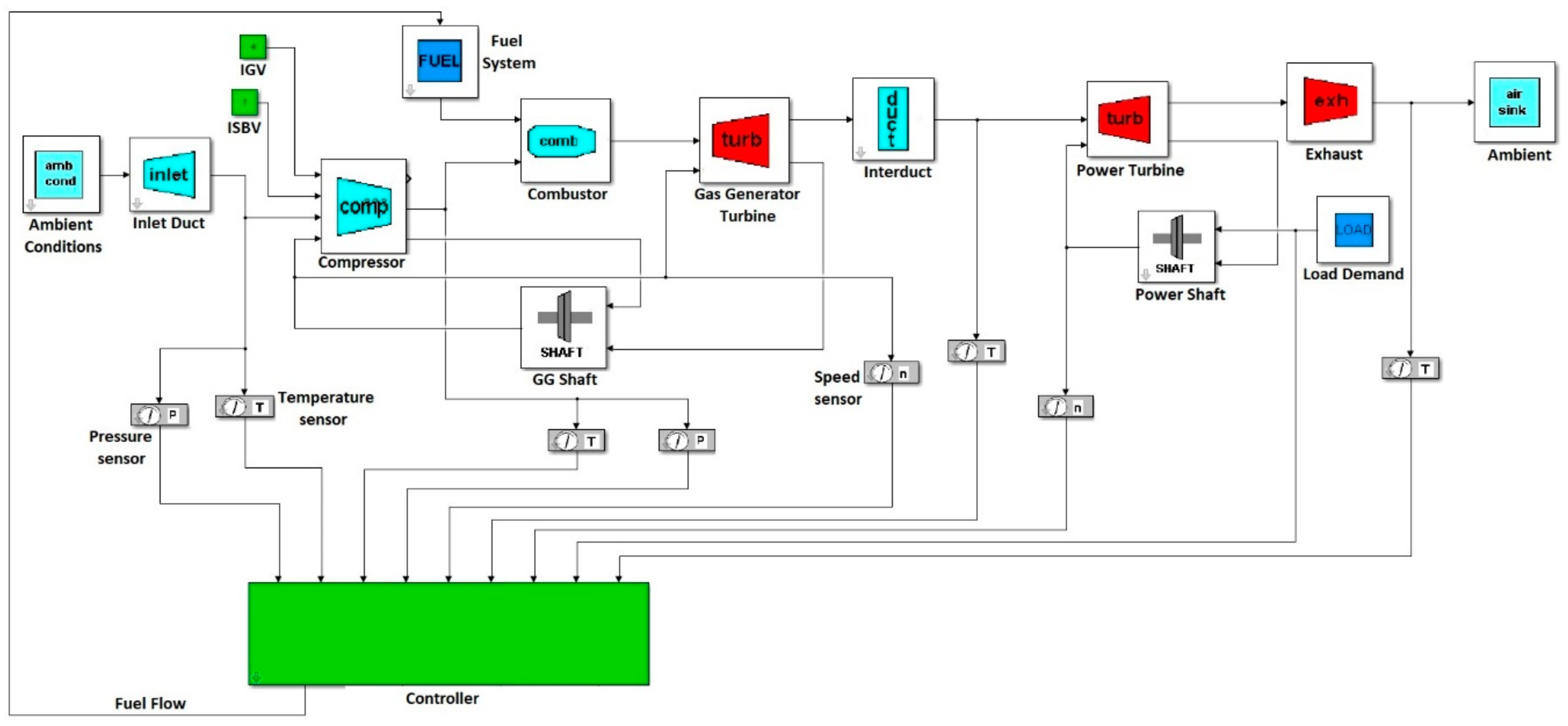
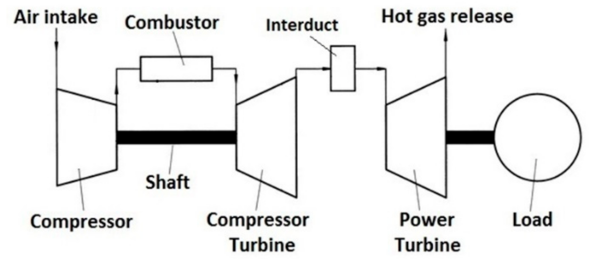
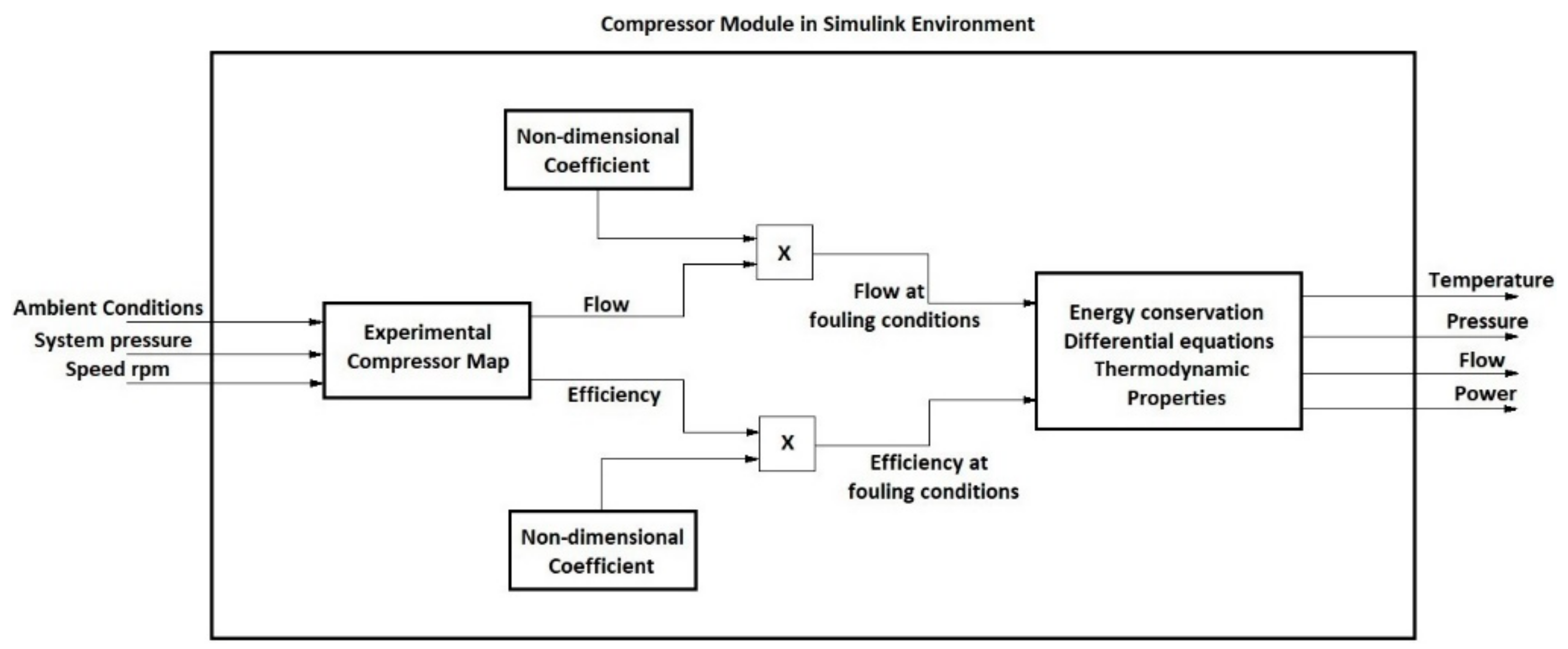
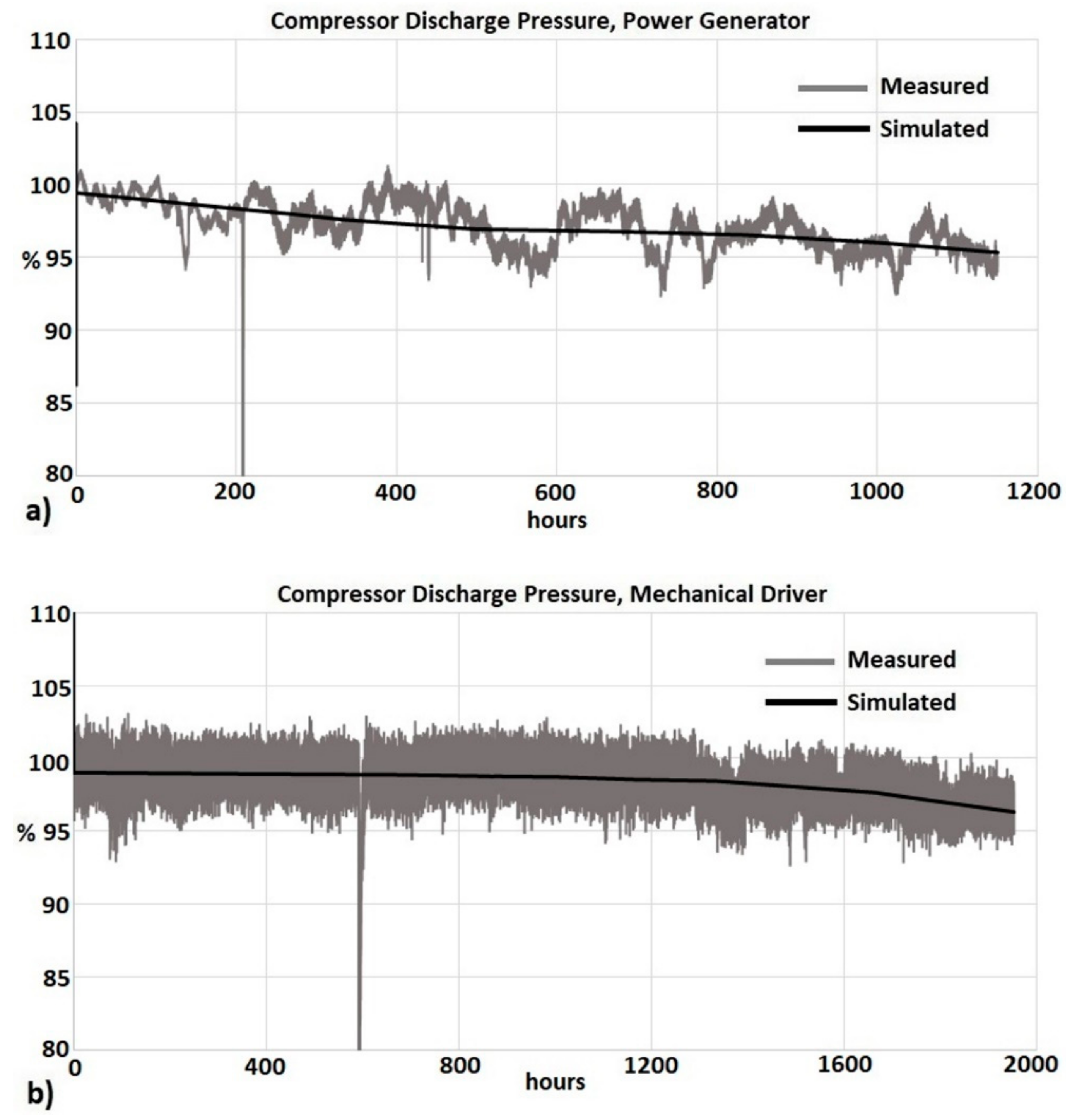
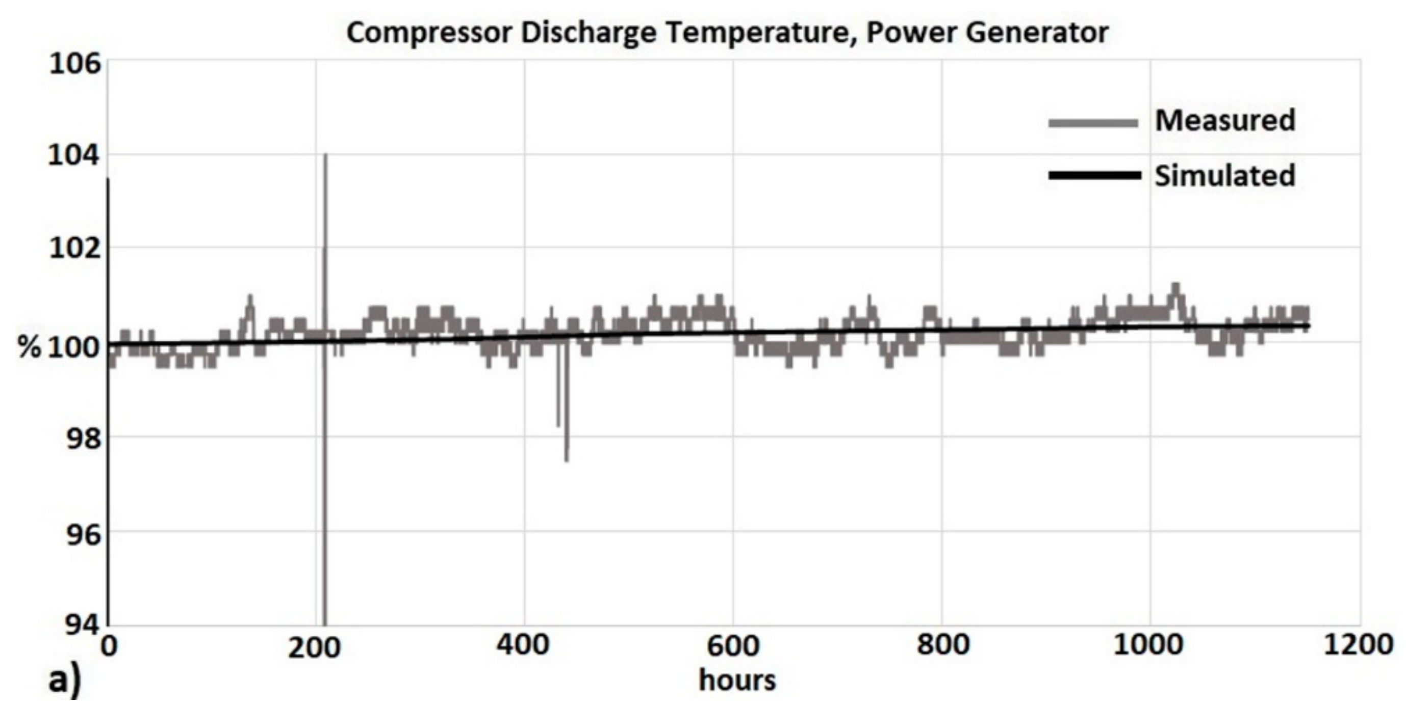
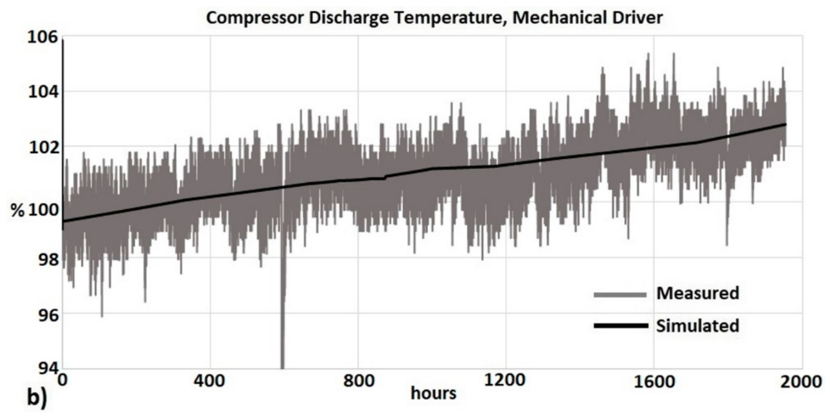
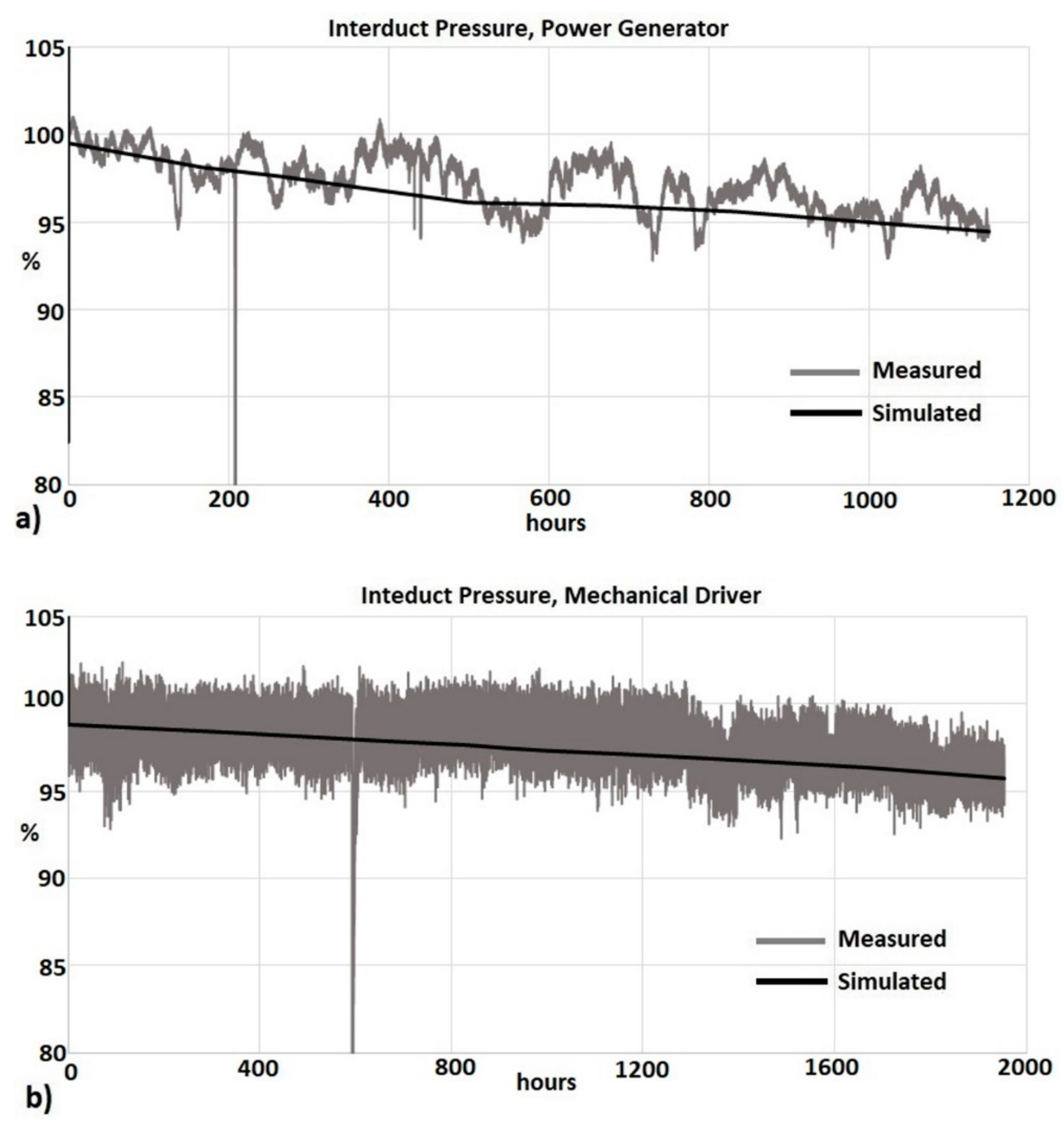
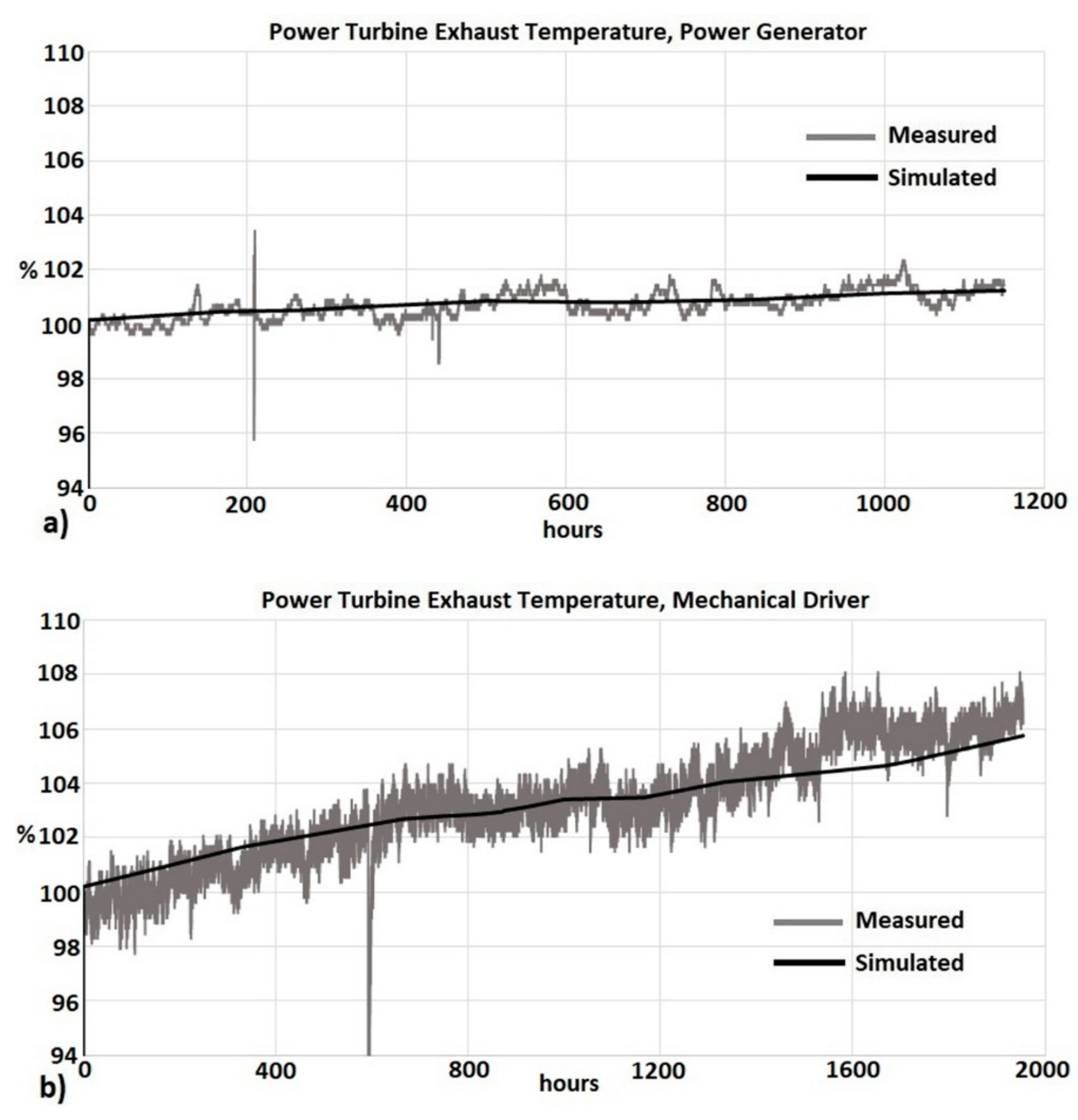
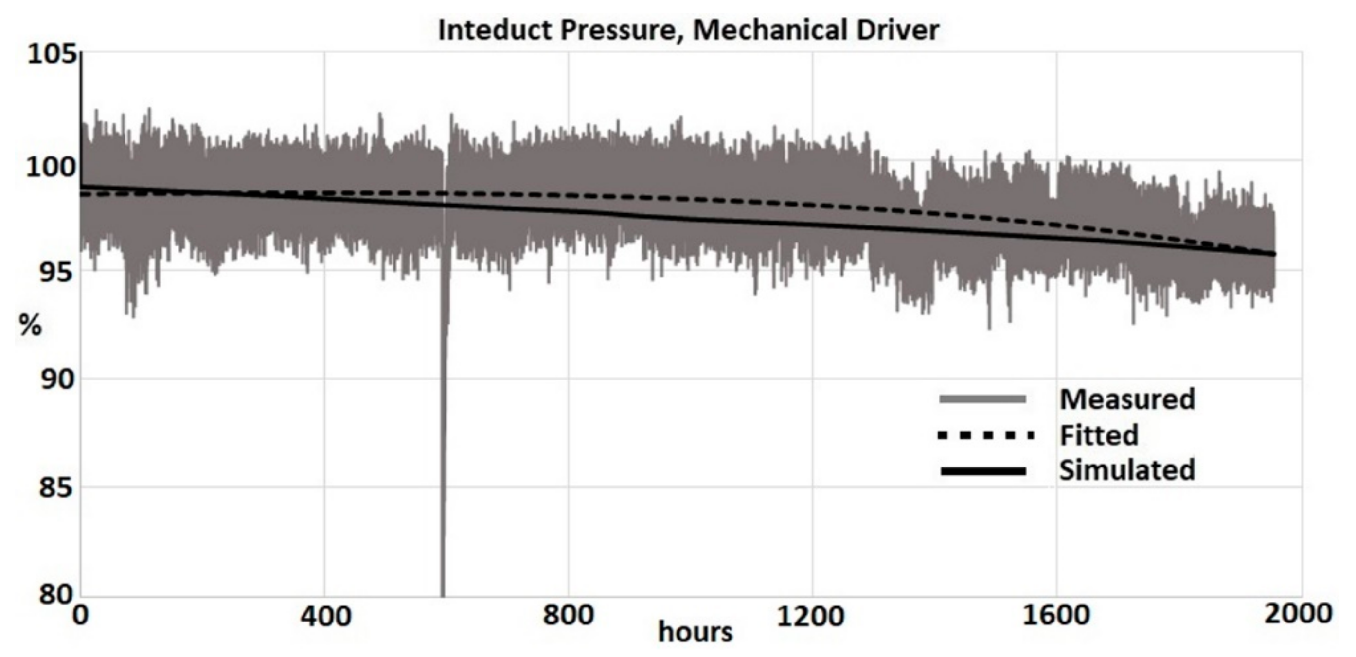
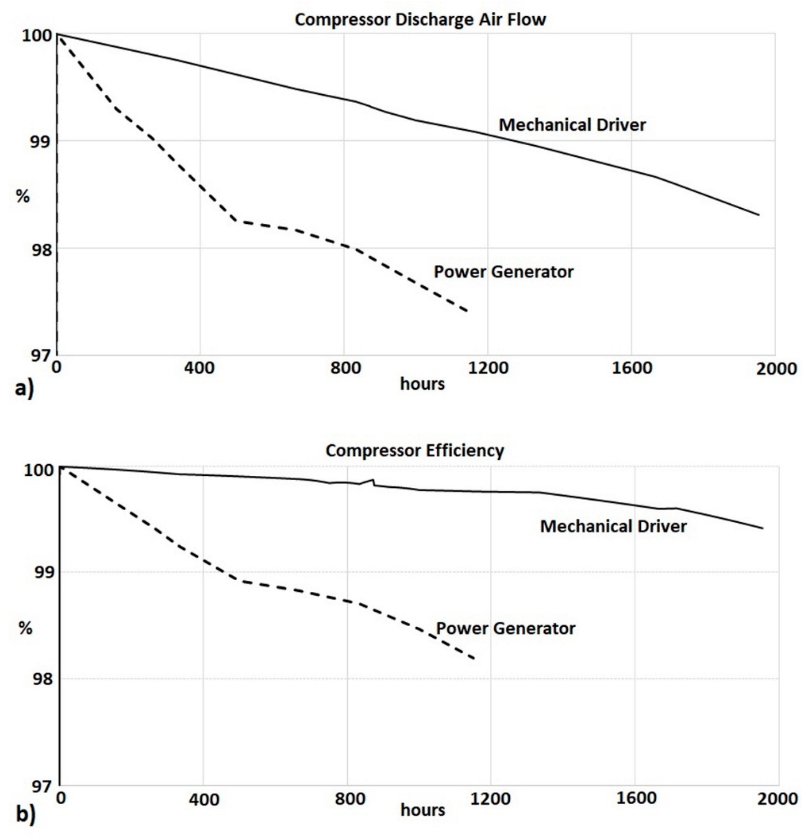
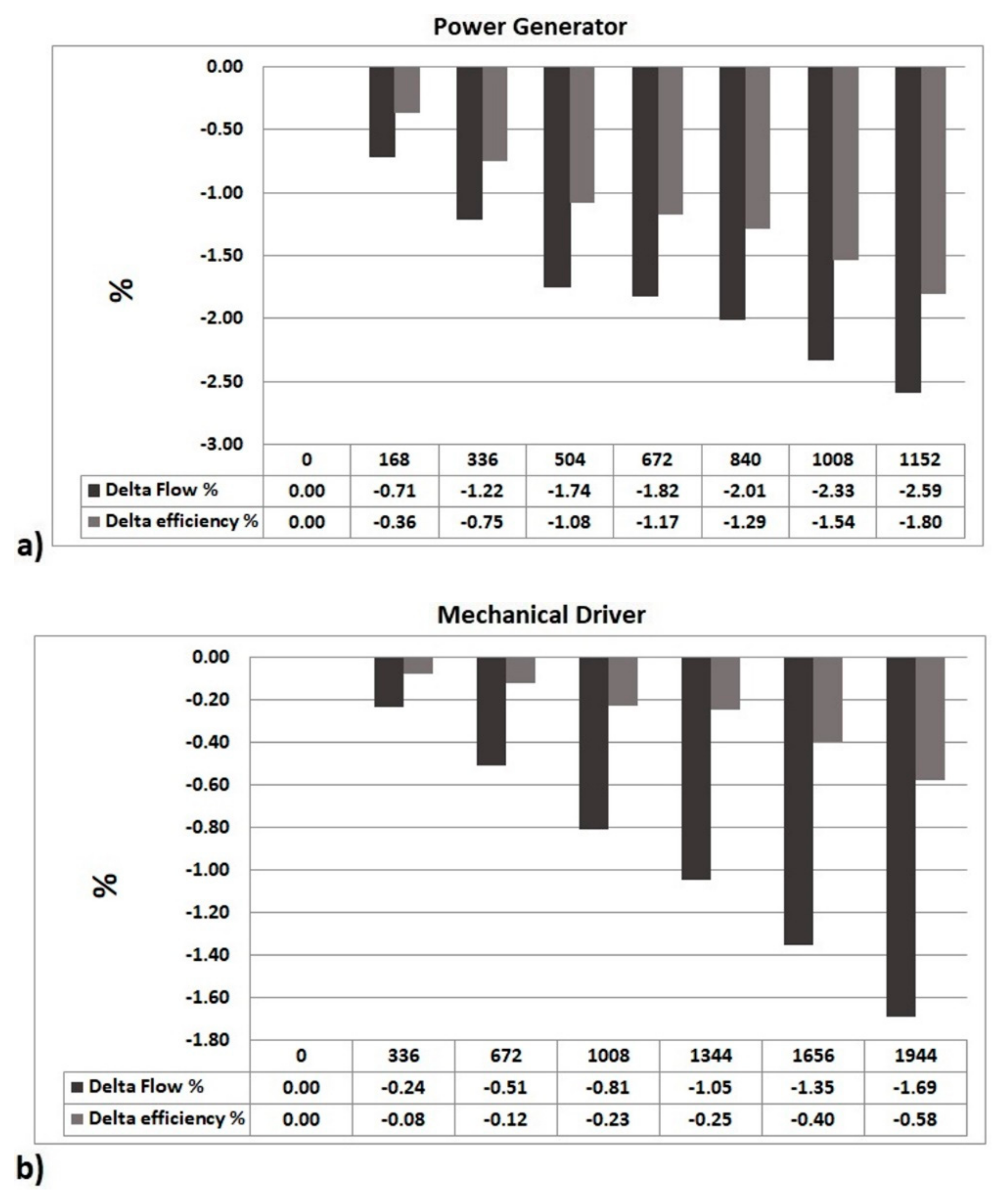
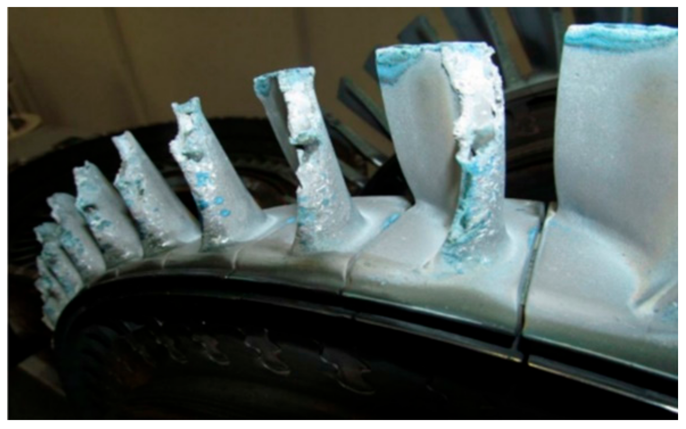
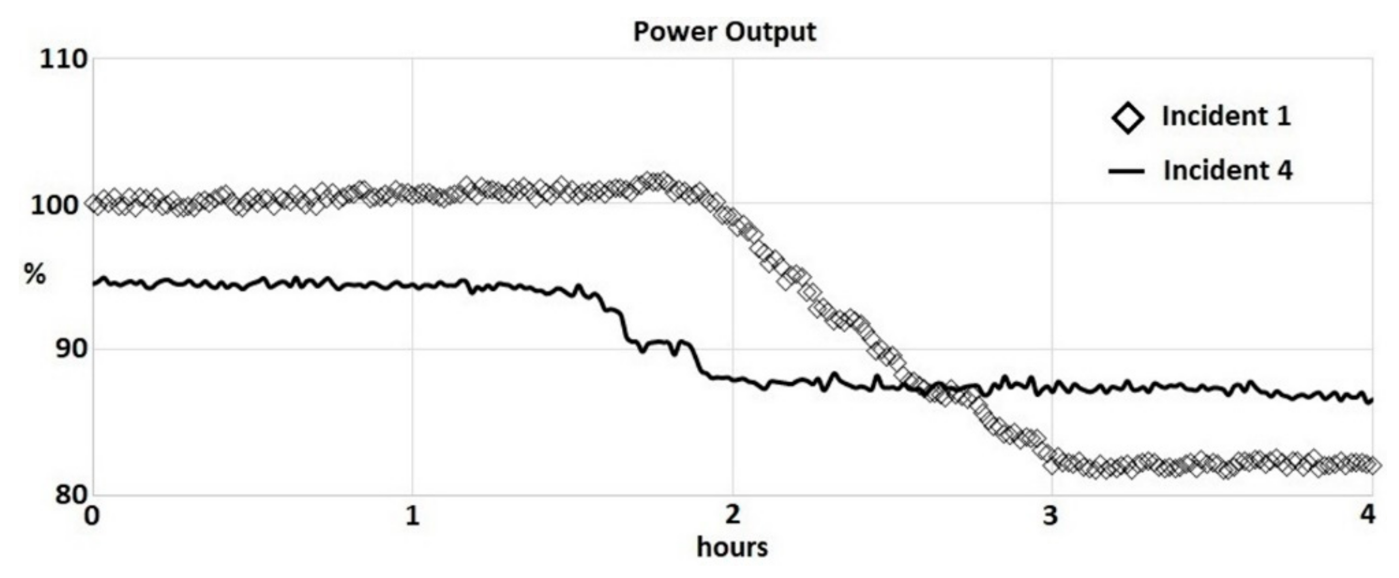
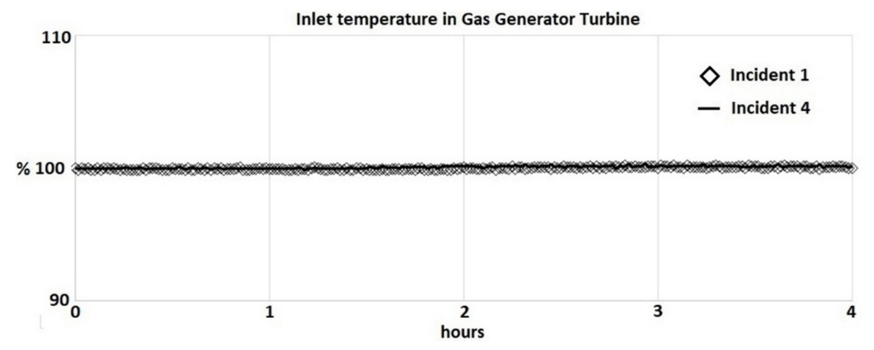
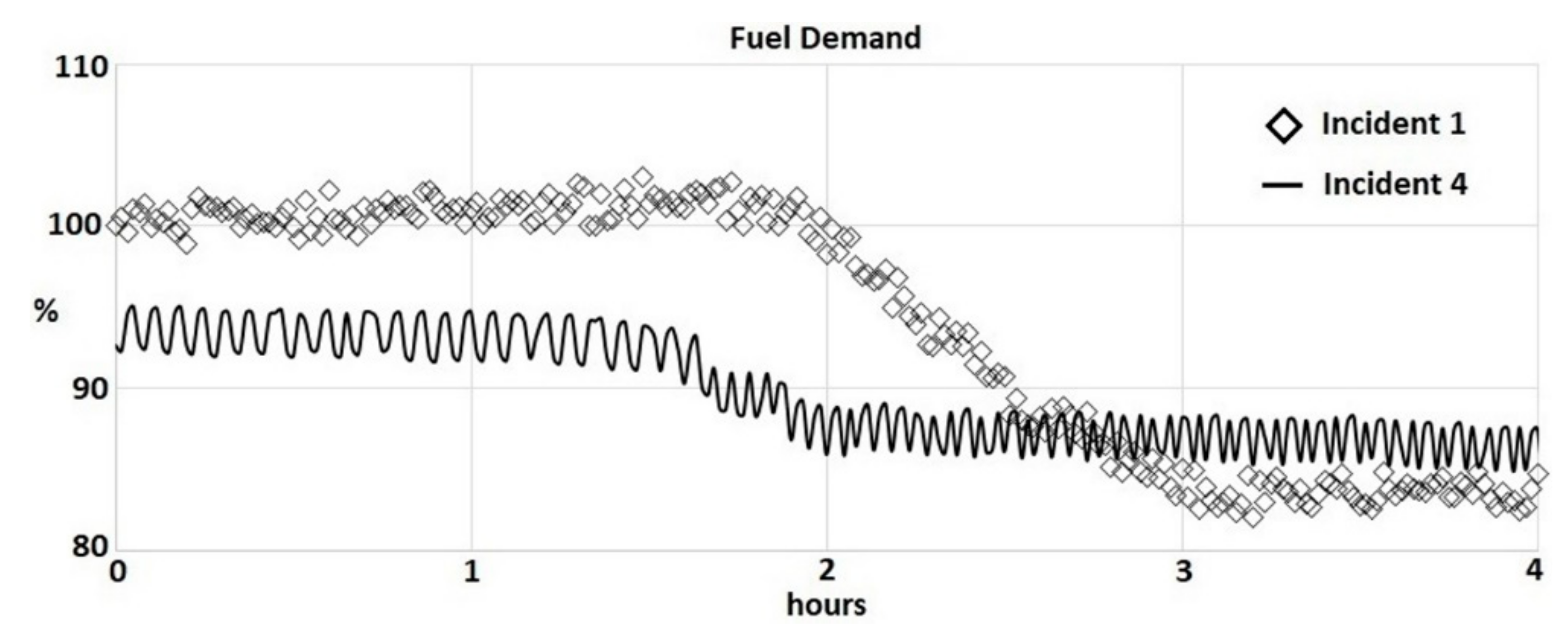
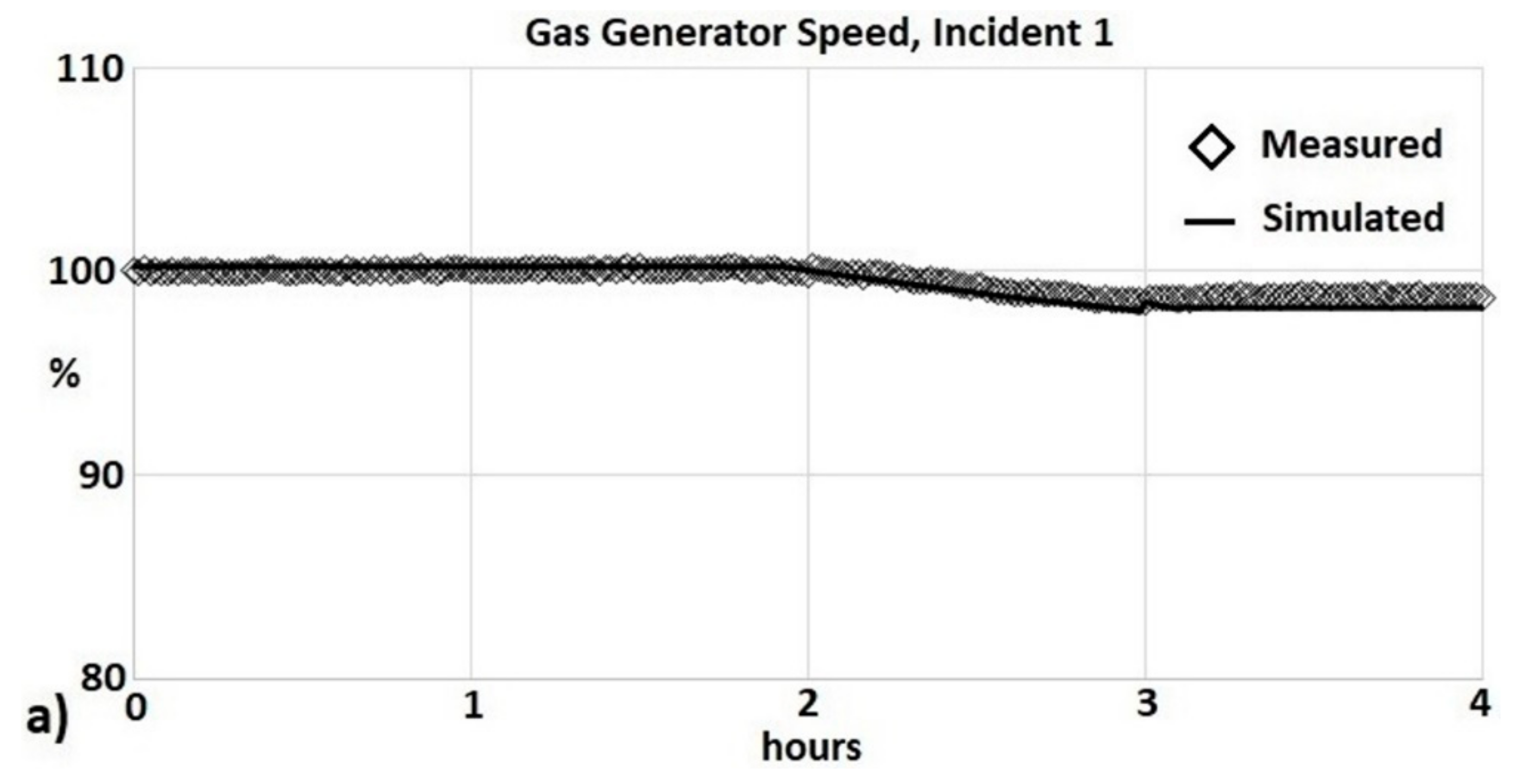
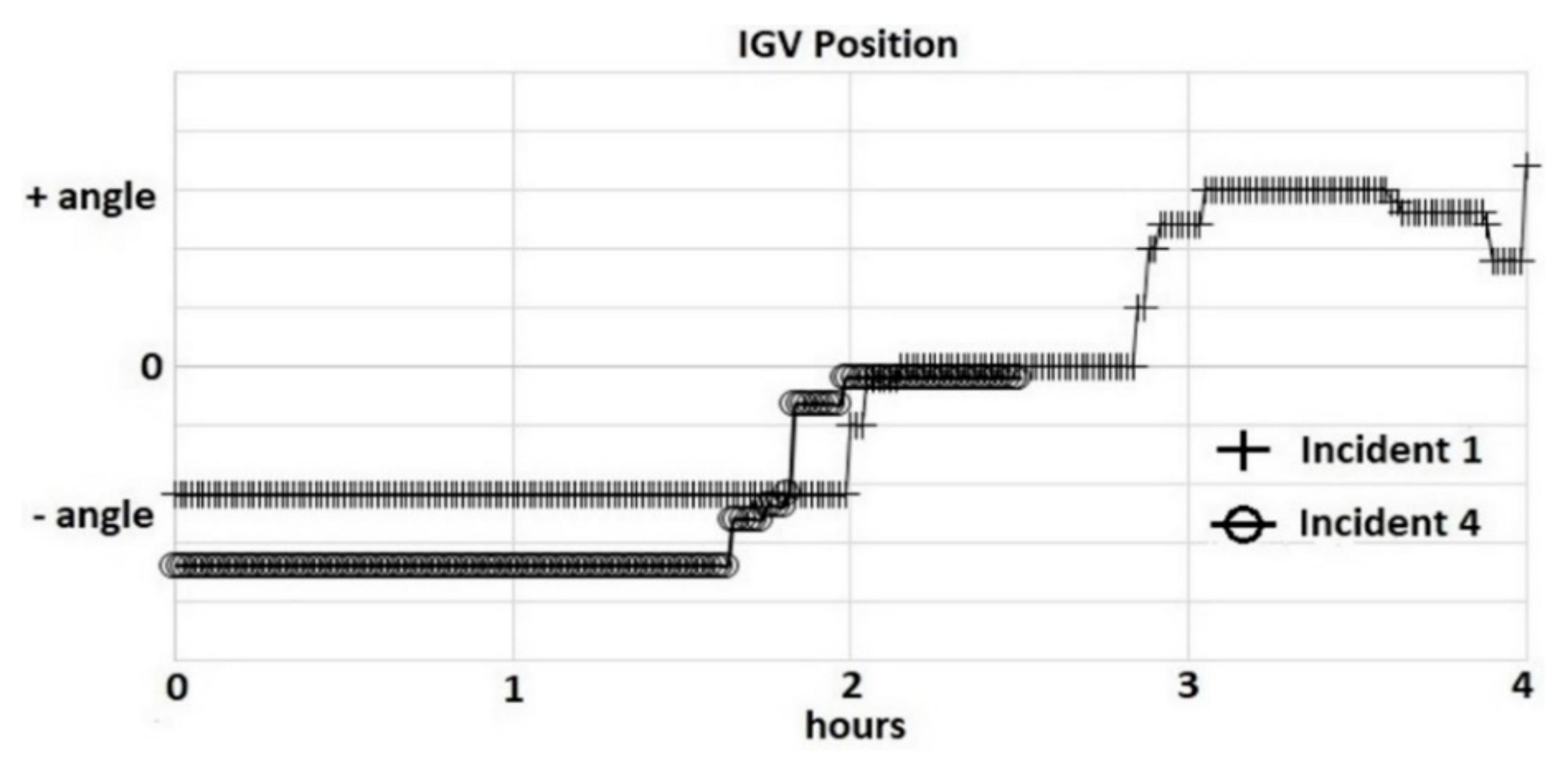
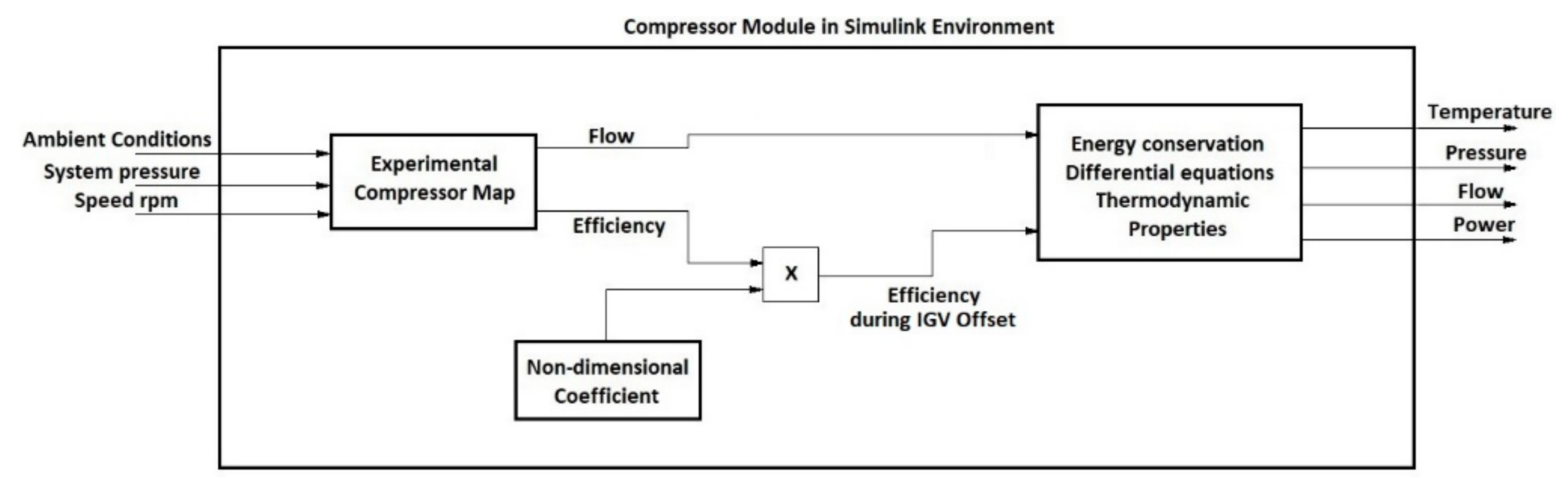
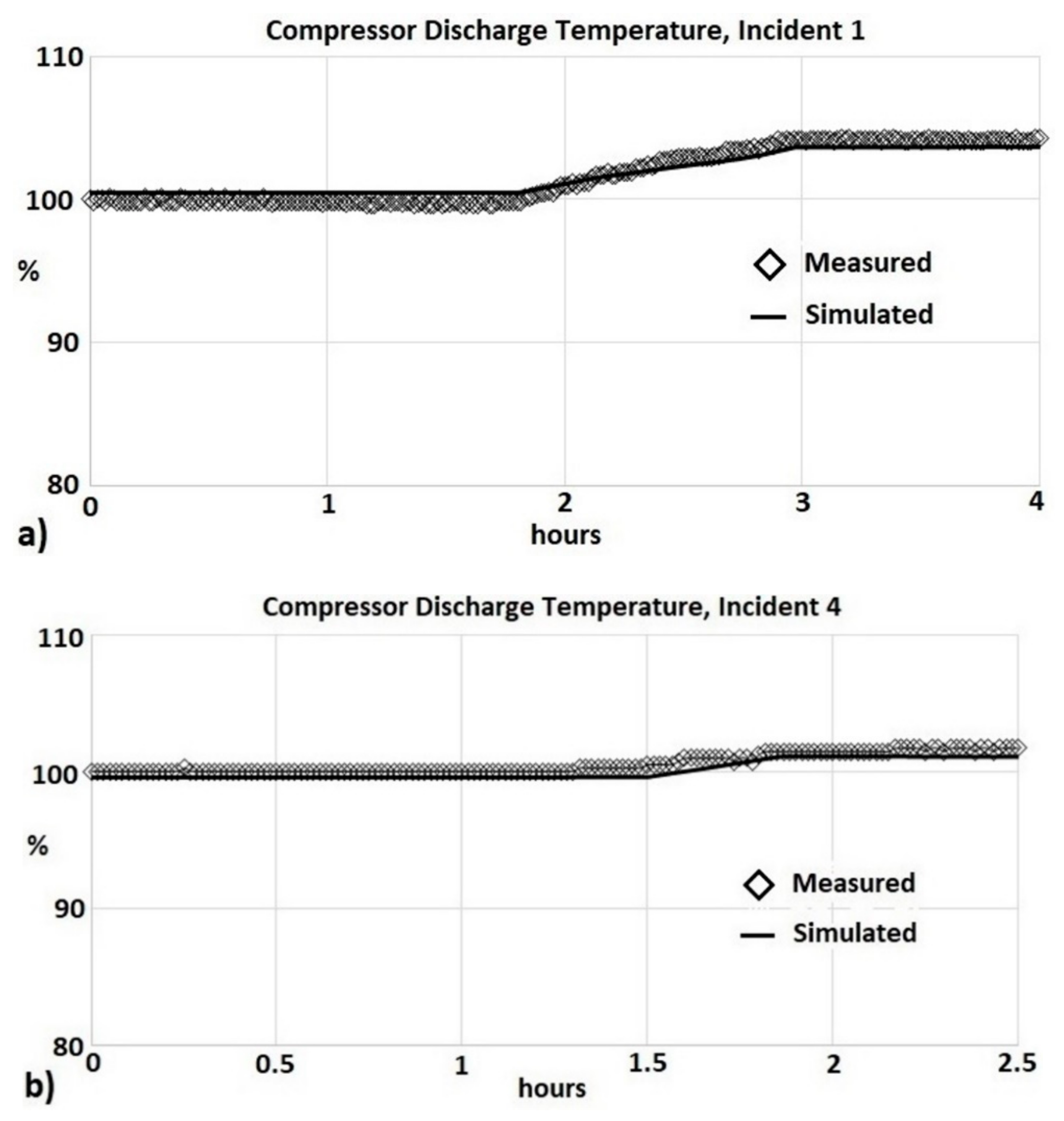
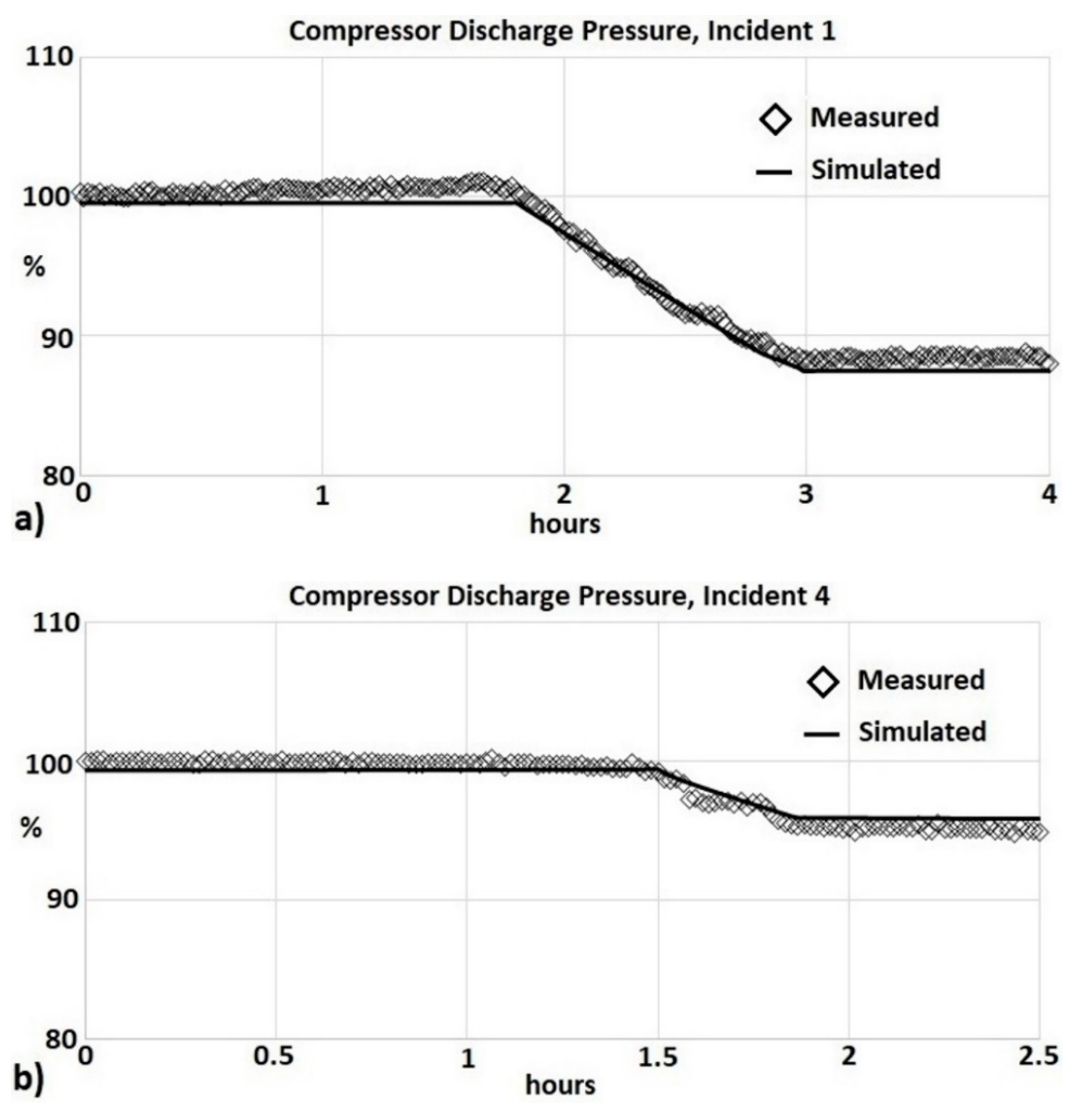
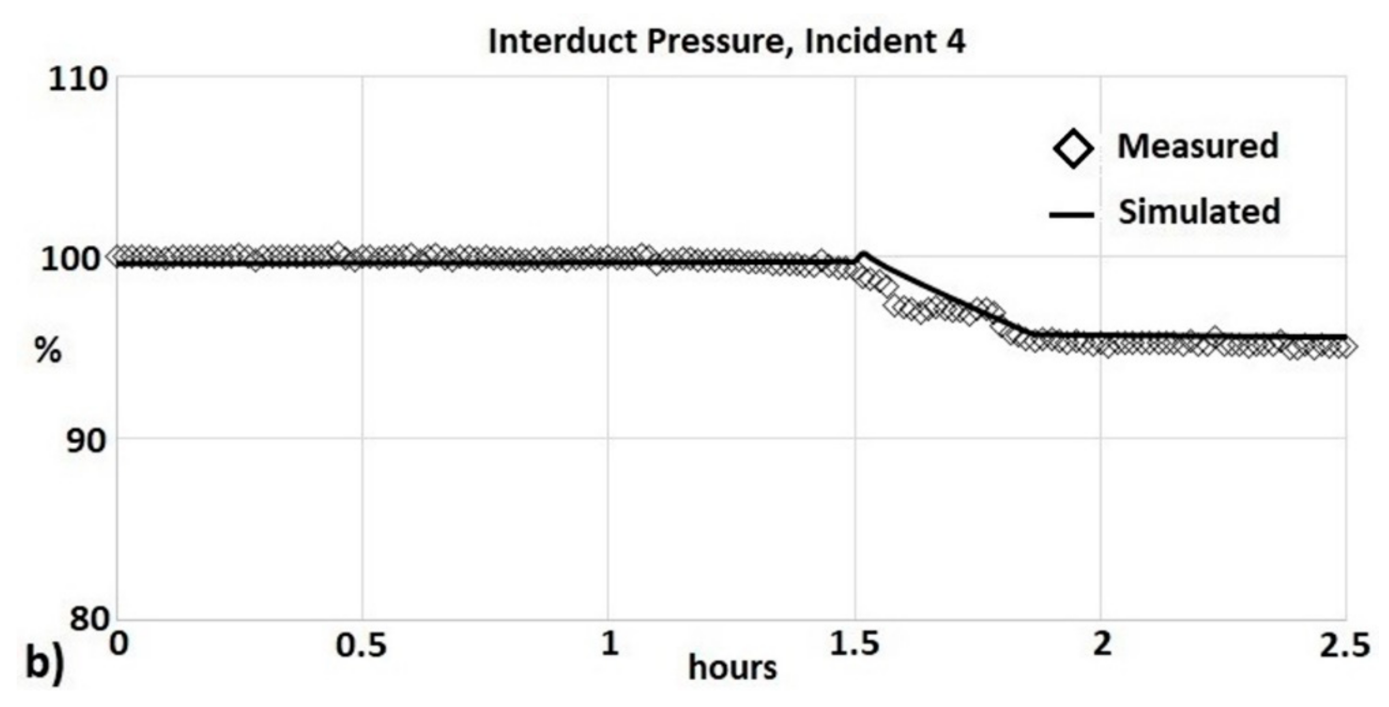
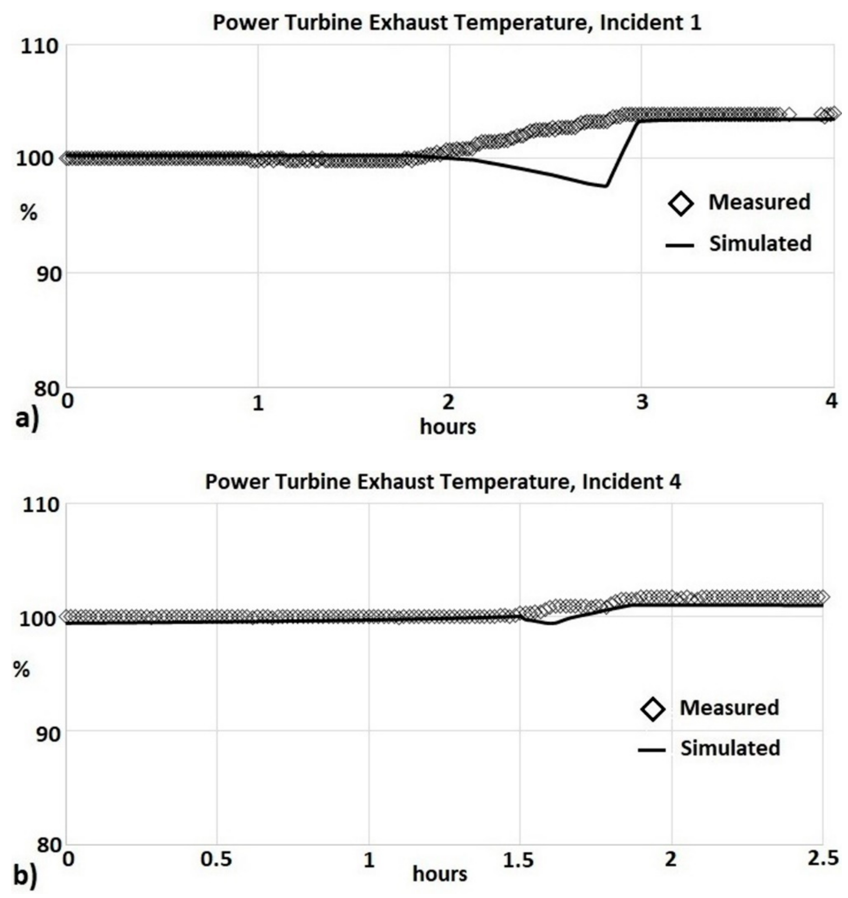
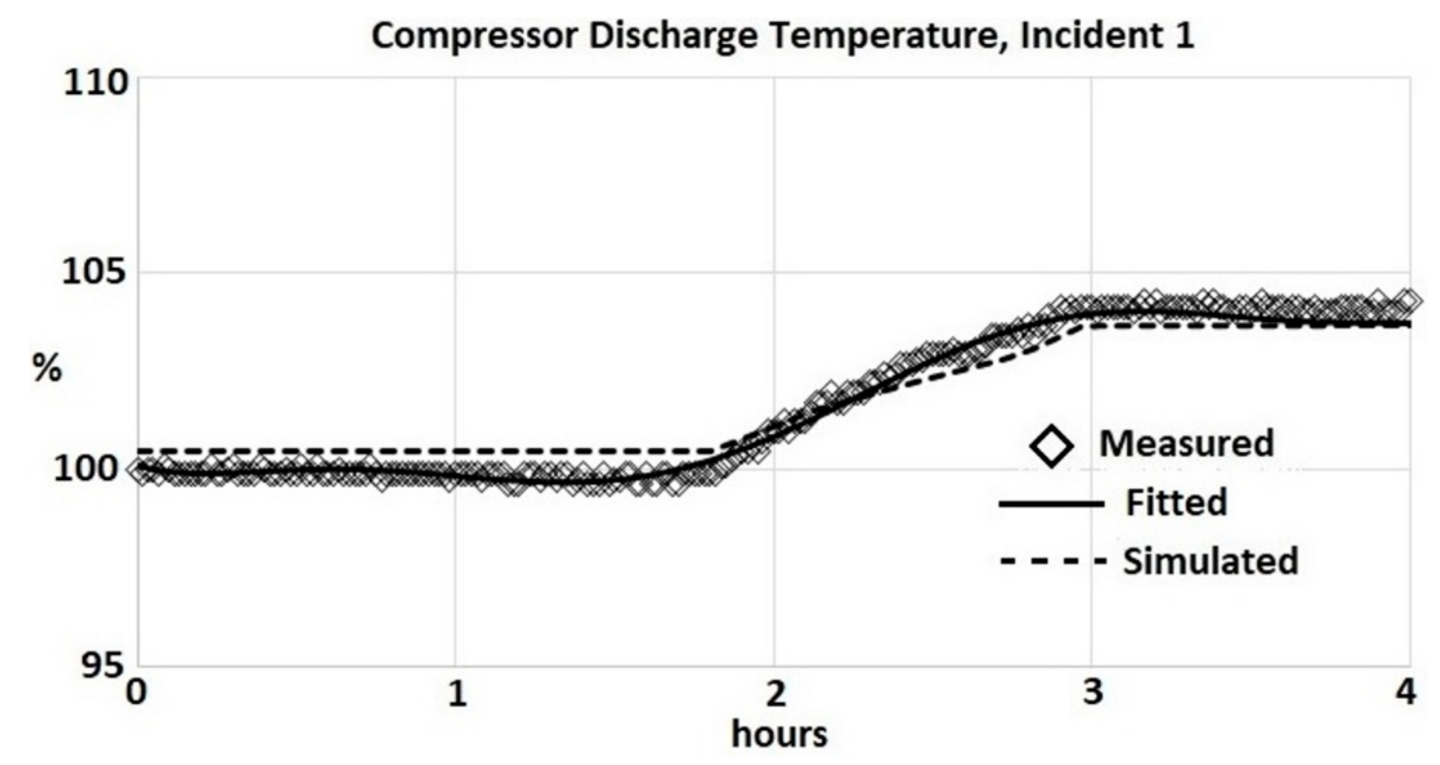
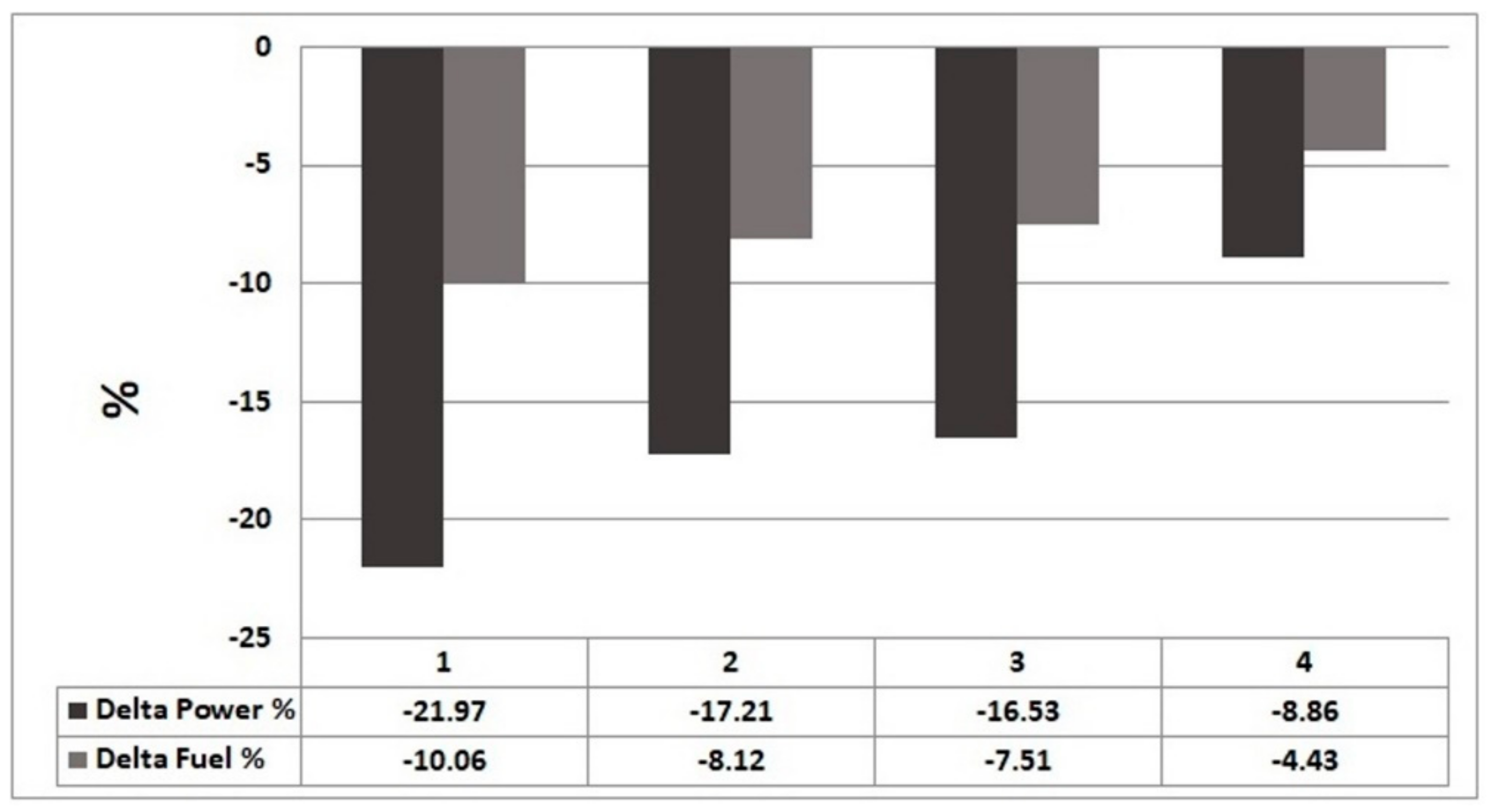
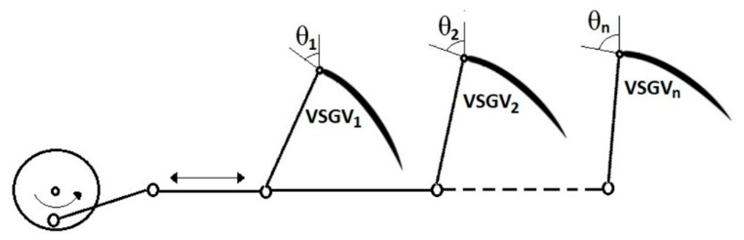
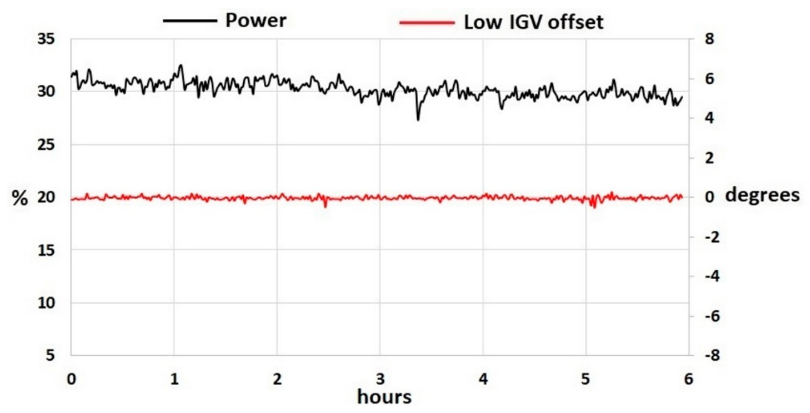
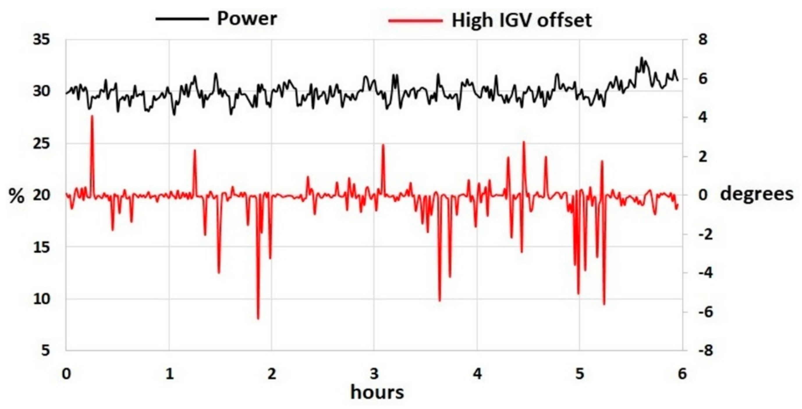
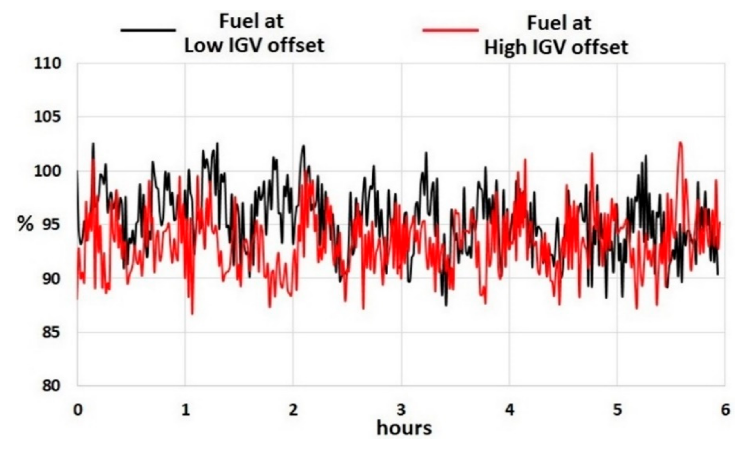
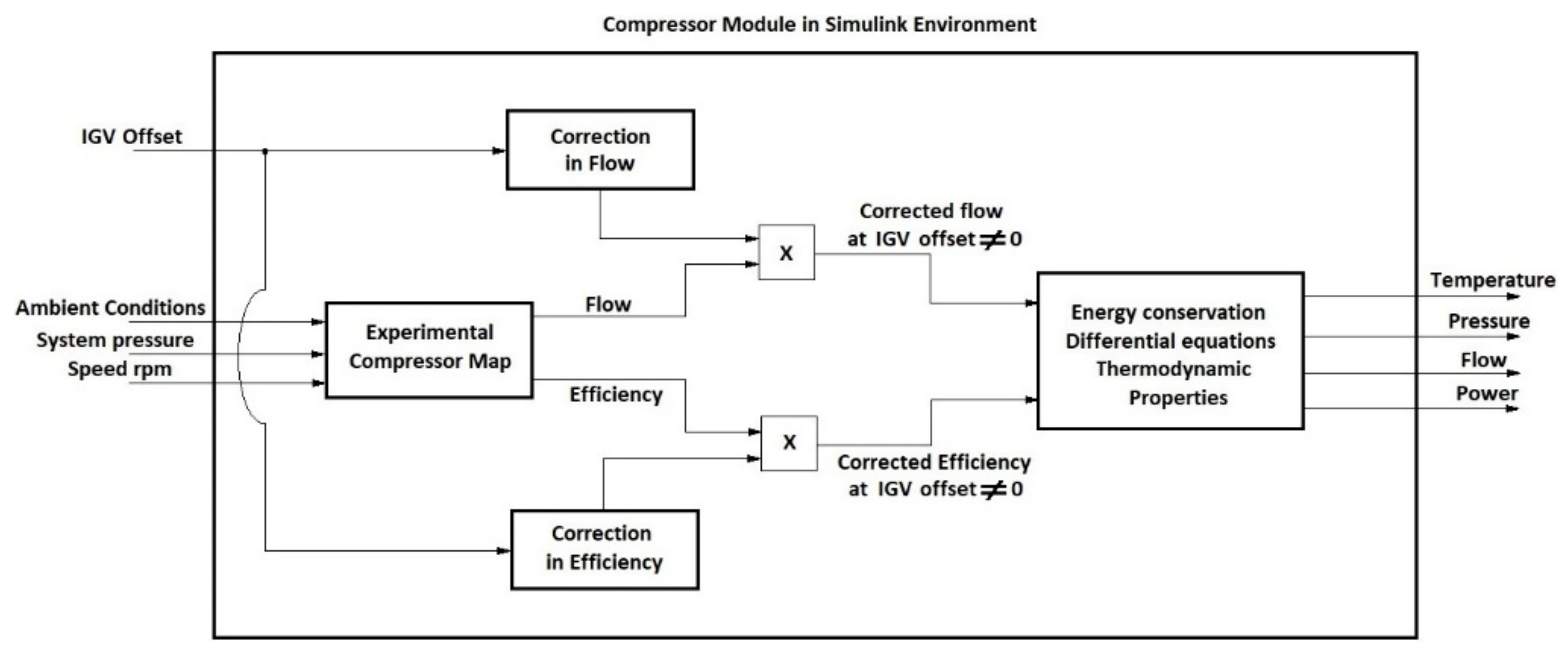
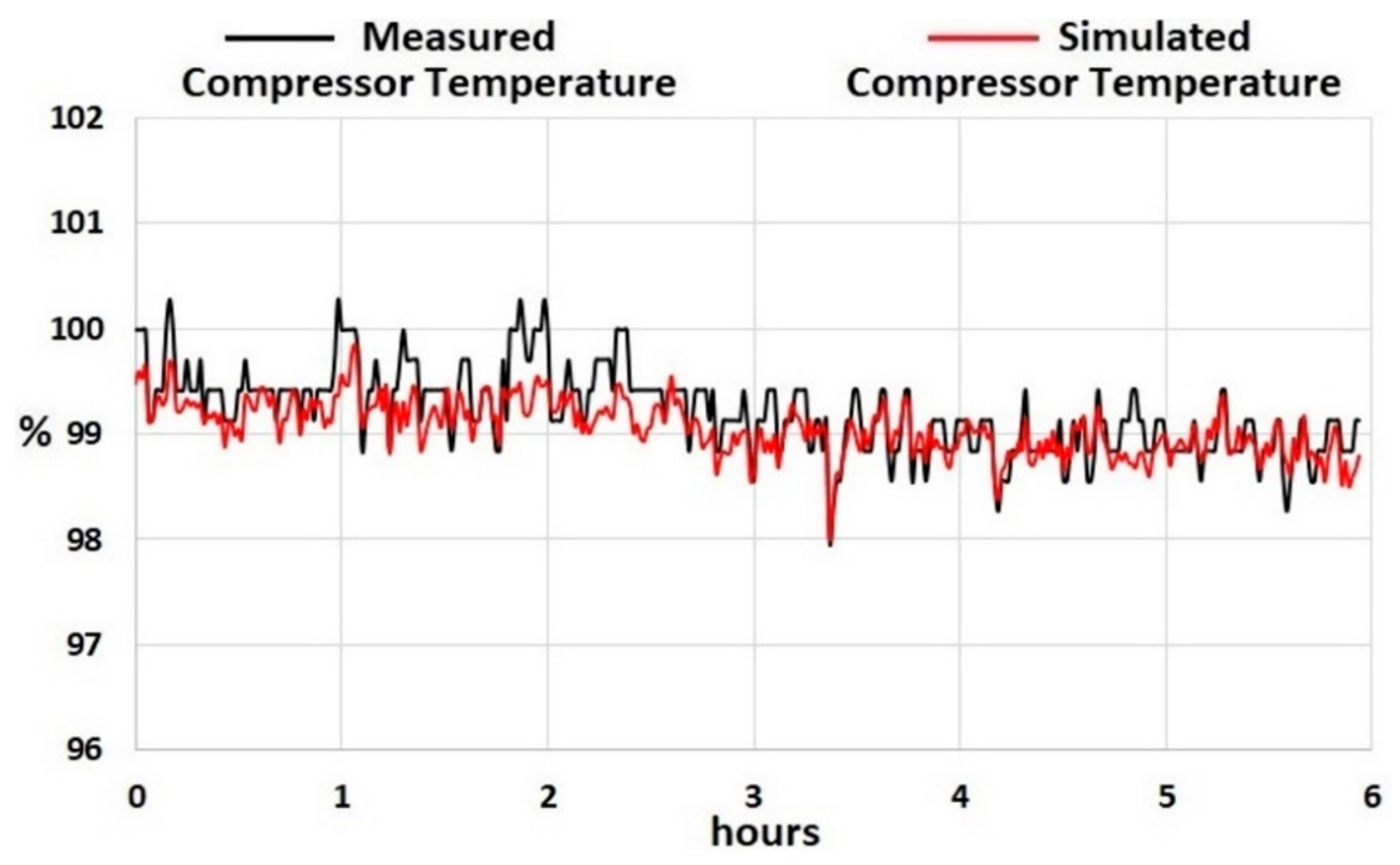
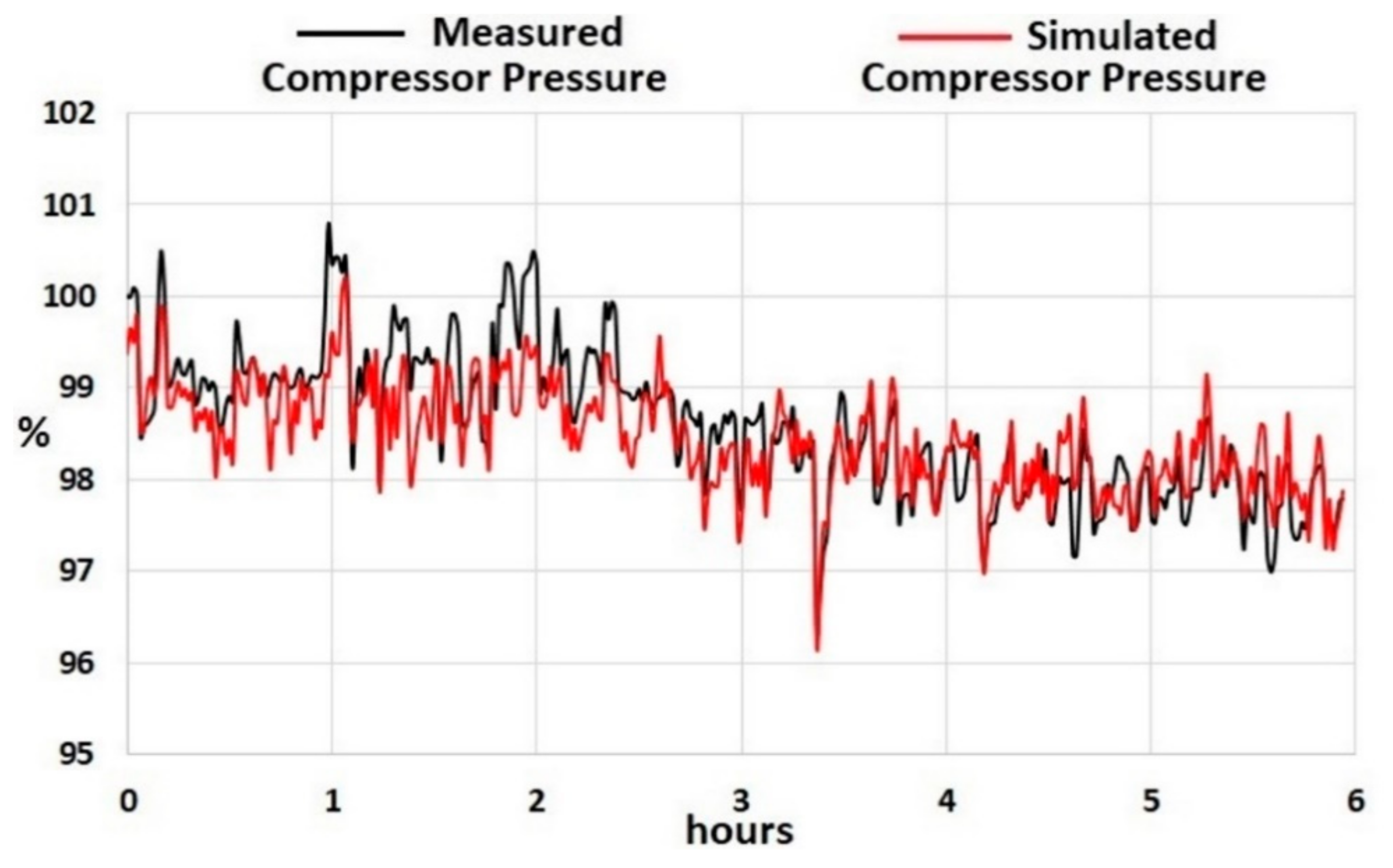
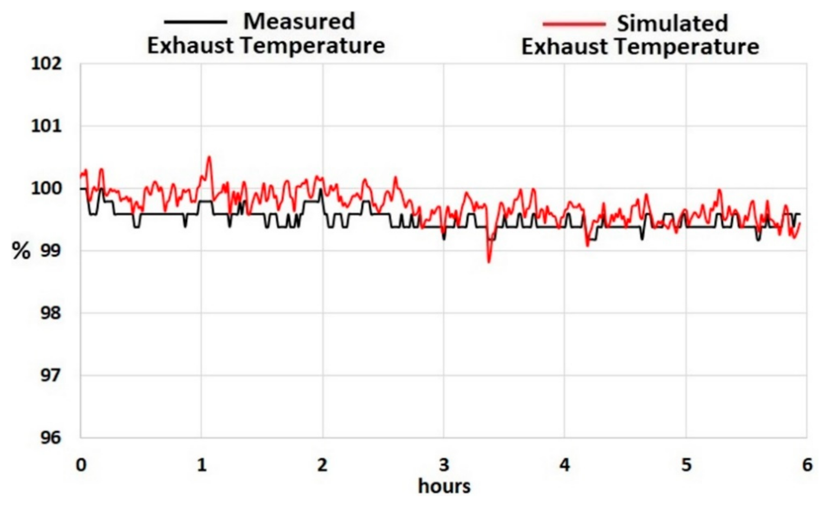
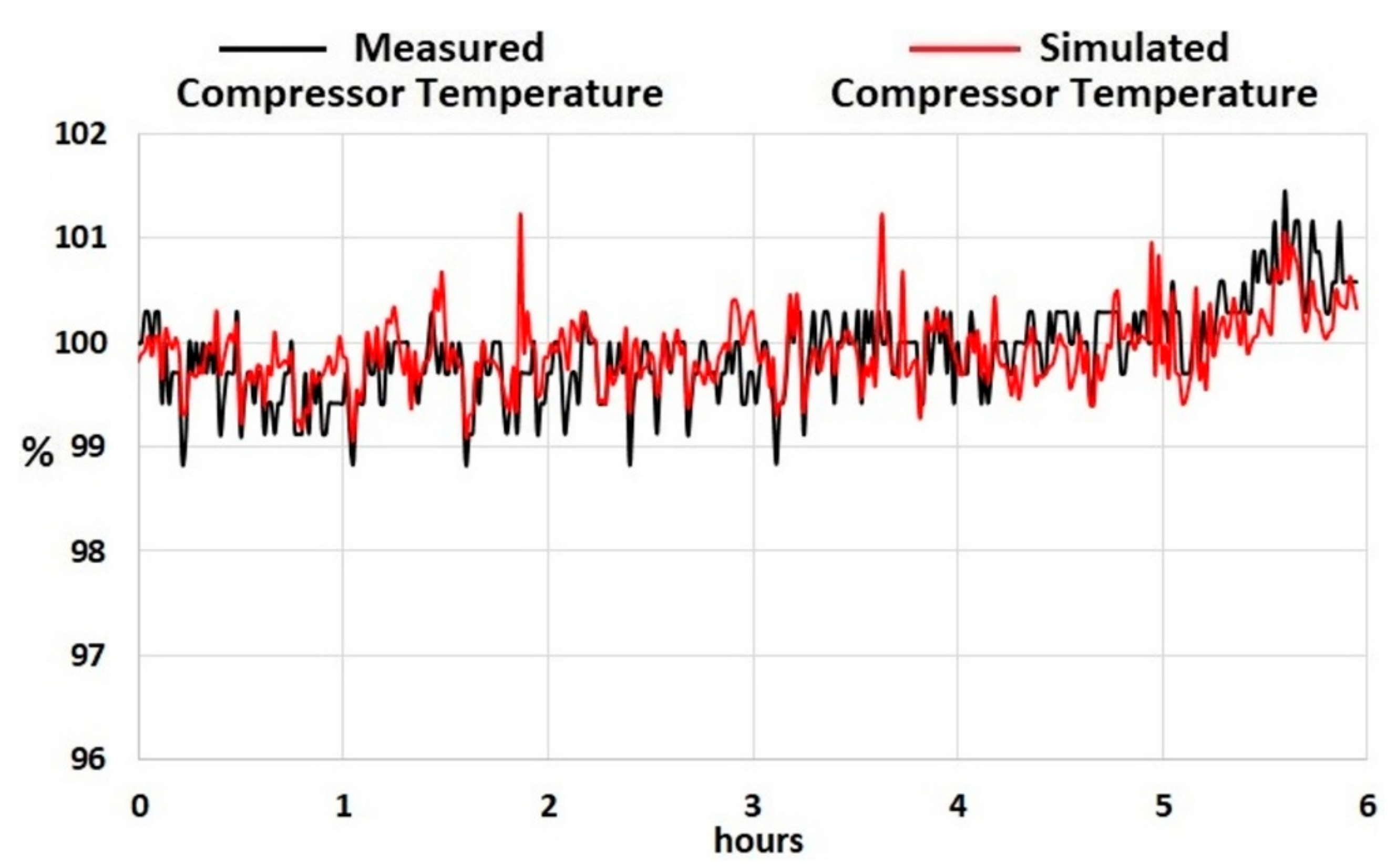
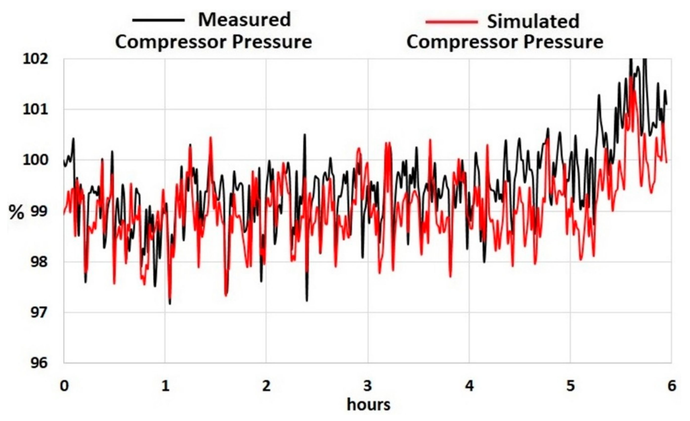
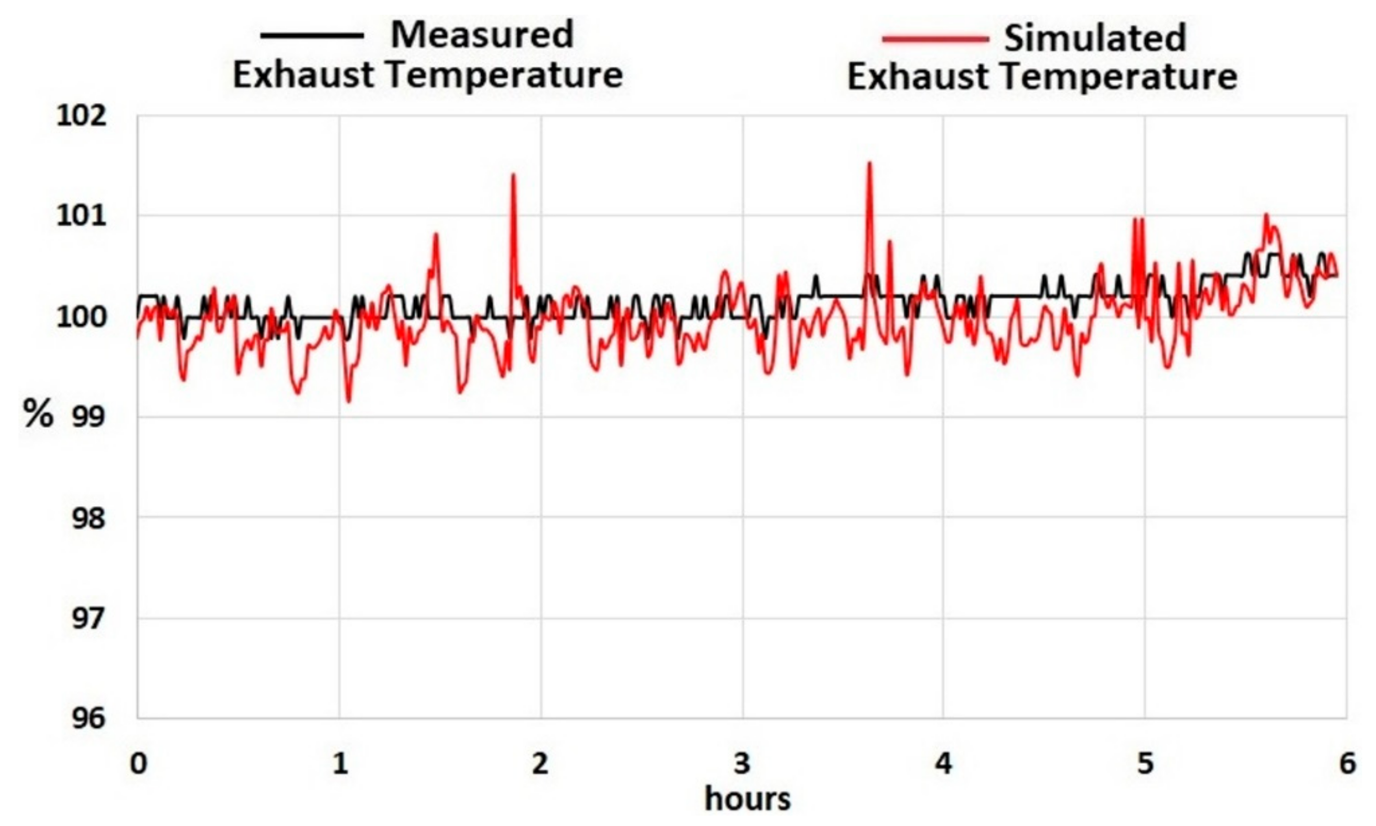
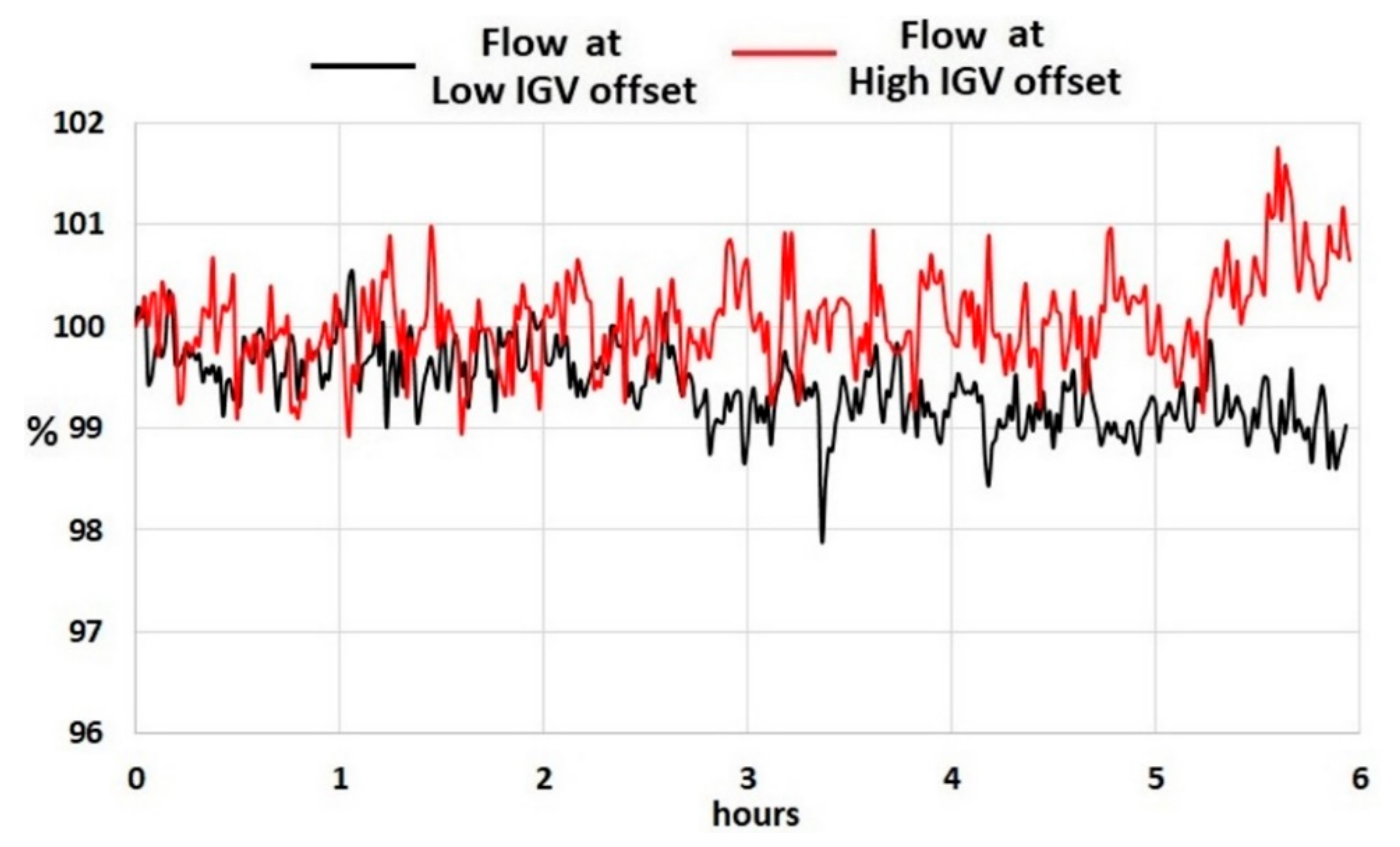
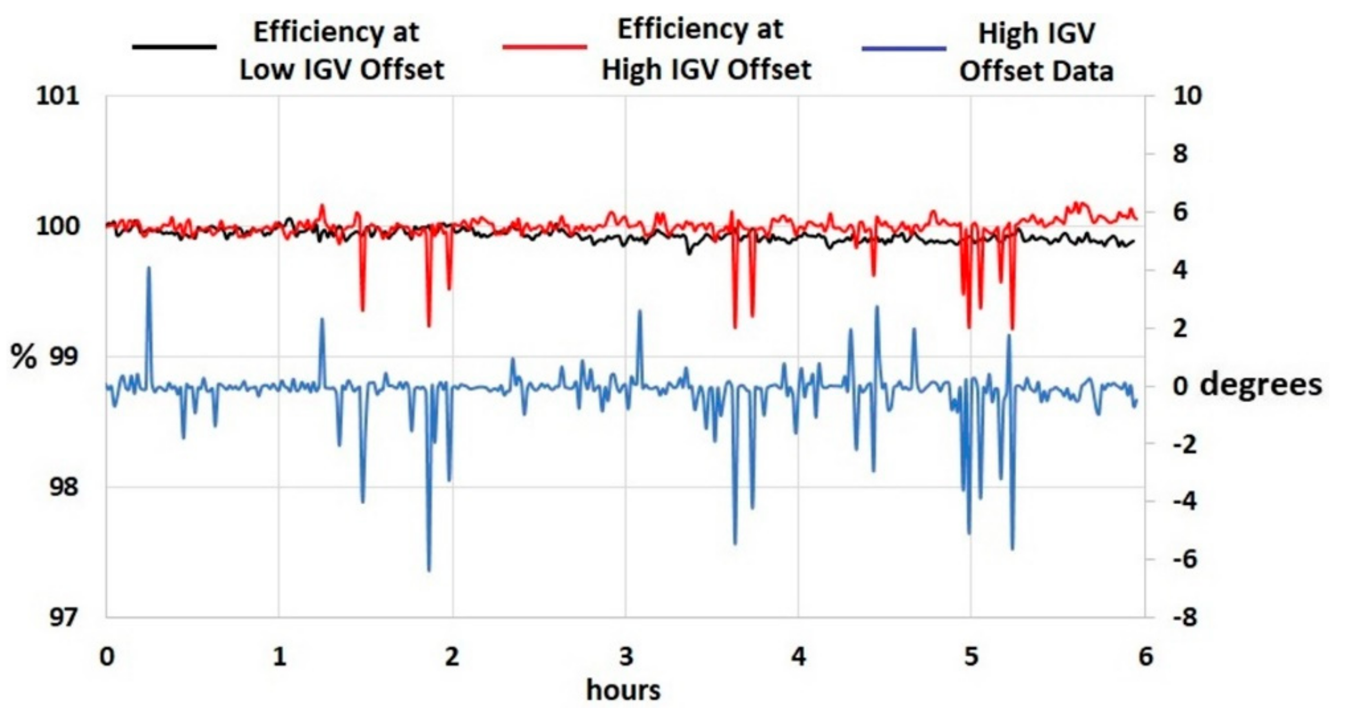
Table 1.
Error between fitted and simulated data at high power operation (power generator).
| Power Generator | ||||
|---|---|---|---|---|
| % Error Compressor | % Error Interduct | % Error Exhaust | ||
| Hours | Discharge Pressure | Discharge Temperature | Pressure | Temperature |
| 0 | 0.0000 | 0.0499 | 0.0000 | 0.0541 |
| 168 | 0.0496 | 0.0585 | 0.3457 | 0.1095 |
| 336 | 0.1799 | 0.0421 | 0.6199 | 0.0430 |
| 504 | 0.3684 | 0.0009 | 1.2334 | 0.0700 |
| 672 | 0.1885 | 0.0095 | 1.0181 | 0.1674 |
| 840 | 0.0245 | 0.0181 | 0.9513 | 0.2219 |
| 1008 | 0.0643 | 0.0267 | 1.0553 | 0.1298 |
| 1152 | 0.0904 | 0.0544 | 0.8735 | 0.1483 |
Table 2.
Error between measured and simulated data at high power operation (power generator).
| Power Generator | ||||
|---|---|---|---|---|
| % Error Compressor | % Error Interduct | % Error Exhaust | ||
| Hours | Discharge Pressure | Discharge Temperature | Pressure | Temperature |
| 0 | 0.5279 | 0.0499 | 0.4945 | 0.1442 |
| 168 | 1.2157 | 0.2488 | 0.6719 | 0.0898 |
| 336 | 0.3892 | 0.1741 | 0.0565 | 0.0718 |
| 504 | 0.5612 | 0.3226 | 1.1026 | 0.0537 |
| 672 | 0.9294 | 0.2239 | 2.1849 | 0.2507 |
| 840 | 0.1867 | 0.2736 | 0.8547 | 0.0000 |
| 1008 | 0.9383 | 0.4208 | 0.2021 | 0.4796 |
| 1152 | 0.8373 | 0.1489 | 0.0291 | 0.2135 |
Table 3.
Error between fitted and simulated data at low power operation (mechanical driver).
| Mechanical Driver | ||||
|---|---|---|---|---|
| % Error Compressor | % Error Interduct | % Error Exhaust | ||
| Hours | Discharge Pressure | Discharge Temperature | Pressure | Temperature |
| 0 | 0.0398 | 0.0334 | 0.2661 | 0.0194 |
| 336 | 0.0426 | 0.0204 | 0.0408 | 0.1978 |
| 672 | 0.0191 | 0.1064 | 0.5151 | 0.4233 |
| 1008 | 0.0567 | 0.2269 | 0.8852 | 0.7063 |
| 1344 | 0.1022 | 0.1582 | 0.8795 | 1.0388 |
| 1656 | 0.1315 | 0.0275 | 0.5150 | 1.5354 |
| 1944 | 0.0353 | 0.0074 | 0.0625 | 1.6798 |
Table 4.
Error between measured and simulated data at low power operation (mechanical driver).
| Mechanical Driver | ||||
|---|---|---|---|---|
| % Error Compressor | % Error Interduct | % Error Exhaust | ||
| Hours | Discharge Pressure | Discharge Temperature | Pressure | Temperature |
| 0 | 0.0829 | 0.1795 | 0.2183 | 0.1887 |
| 336 | 0.3234 | 0.0765 | 0.2197 | 0.0372 |
| 672 | 0.5062 | 0.8543 | 0.0368 | 1.7754 |
| 1008 | 0.8979 | 0.4285 | 1.7103 | 0.3650 |
| 1344 | 0.8833 | 0.5525 | 0.0372 | 0.8484 |
| 1656 | 0.0420 | 0.0250 | 0.7053 | 1.8650 |
| 1944 | 1.6184 | 0.7444 | 1.5807 | 1.1858 |
Table 5.
Error between fitted and simulated data for compressor discharge temperature, compressor discharge pressure, interduct pressure, and exhaust temperature for the four GGT damage incidents at steady-state.
Table 5.
Error between fitted and simulated data for compressor discharge temperature, compressor discharge pressure, interduct pressure, and exhaust temperature for the four GGT damage incidents at steady-state.
| %Steady-State Error | |||||
|---|---|---|---|---|---|
| Incident | Compressor Pressure | Compressor Temperature | Interduct Pressure | Exhaust Temperature | |
| 1 | Initial Condition | 0.74 | 0.31 | 0.522 | 0.36 |
| GGT Damage | 0.24 | 0.34 | 1.11 | 0.18 | |
| 2 | Initial Condition | 0.147 | 0.1 | 0.57 | 0.128 |
| GGT Damage | 0.2 | 0.054 | 1.4 | 0.018 | |
| 3 | Initial Condition | 0.267 | 0.048 | 0.205 | 0.092 |
| GGT Damage | 0.282 | 0.237 | 0.49 | 0.722 | |
| 4 | Initial Condition | 0.31 | 0.01 | 0.19 | 0.16 |
| GGT Damage | 0.959 | 0.71 | 0.26 | 0.43 | |
Table 6.
Error between measured and simulated data for compressor discharge temperature, compressor discharge pressure, interduct pressure, and exhaust temperature for the four GGT damage incidents at steady-state.
Table 6.
Error between measured and simulated data for compressor discharge temperature, compressor discharge pressure, interduct pressure, and exhaust temperature for the four GGT damage incidents at steady-state.
| % Steady-State Error | |||||
|---|---|---|---|---|---|
| Incident | Compressor Pressure | Compressor Temperature | Interduct Pressure | Exhaust Temperature | |
| 1 | Initial Condition | 0.267 | 0.48 | 0.205 | 0.92 |
| GGT Damage | 0.282 | 0.237 | 0.490 | 0.722 | |
| 2 | Initial Condition | 0.147 | 0.11 | 0.577 | 0.128 |
| GGT Damage | 0.12 | 0.541 | 1.406 | 0.182 | |
| 3 | Initial Condition | 0.741 | 0.314 | 0.522 | 0.36 |
| GGT Damage | 0.244 | 0.343 | 1.111 | 0.183 | |
| 4 | Initial Condition | 0.743 | 0.312 | 0.522 | 0.36 |
| GGT Damage | 0.241 | 0.343 | 1.121 | 0.18 | |
Table 7.
Error between measured and simulated data for different IGV offset values.
| IGV Offset | % GGS | % CDT | % CDP | % ET |
|---|---|---|---|---|
| 4.1 | 0.298 | 0.299 | 0.663 | 0.351 |
| 2.3 | 0.079 | 0.342 | 0.052 | 0.102 |
| −3.98 | 0.700 | 0.673 | 0.527 | 0.816 |
| −6.4 | 0.739 | 1.506 | 0.322 | 1.387 |
© 2018 by the authors. Licensee MDPI, Basel, Switzerland. This article is an open access article distributed under the terms and conditions of the Creative Commons Attribution (CC BY) license (http://creativecommons.org/licenses/by/4.0/).
Share and Cite
MDPI and ACS Style
Cruz-Manzo, S.; Panov, V.; Zhang, Y. Gas Path Fault and Degradation Modelling in Twin-Shaft Gas Turbines. Machines 2018, 6, 43. https://doi.org/10.3390/machines6040043
AMA Style
Cruz-Manzo S, Panov V, Zhang Y. Gas Path Fault and Degradation Modelling in Twin-Shaft Gas Turbines. Machines. 2018; 6(4):43. https://doi.org/10.3390/machines6040043
Chicago/Turabian StyleCruz-Manzo, Samuel, Vili Panov, and Yu Zhang. 2018. "Gas Path Fault and Degradation Modelling in Twin-Shaft Gas Turbines" Machines 6, no. 4: 43. https://doi.org/10.3390/machines6040043
Note that from the first issue of 2016, this journal uses article numbers instead of page numbers. See further details here.