Tracking and Counting of Tomato at Different Growth Period Using an Improving YOLO-Deepsort Network for Inspection Robot

Abstract

To realize tomato growth period monitoring and yield prediction of tomato cultivation, our study proposes a visual object tracking network called YOLO-deepsort to identify and count tomatoes in different growth periods. Based on the YOLOv5s model, our model uses shufflenetv2, combined with the CBAM attention mechanism, to compress the model size from the algorithm level. In the neck part of the network, the BiFPN multi-scale fusion structure is used to improve the prediction accuracy of the network. When the target detection network completes the bounding box prediction of the target, the Kalman filter algorithm is used to predict the target’s location in the next frame, which is called the tracker in this paper. Finally, calculate the bounding box error between the predicted bounding box and the bounding box output by the object detection network to update the parameters of the Kalman filter and repeat the above steps to achieve the target tracking of tomato fruits and flowers. After getting the tracking results, we use OpenCV to create a virtual count line to count the targets. Our algorithm achieved a competitive result based on the above methods: The mean average precision of flower, green tomato, and red tomato was 93.1%, 96.4%, and 97.9%. Moreover, we demonstrate the tracking ability of the model and the counting process by counting tomato flowers. Overall, the YOLO-deepsort model could fulfill the actual requirements of tomato yield forecast in the greenhouse scene, which provide theoretical support for crop growth status detection and yield forecast.

1. Introduction

The development of facility agriculture enables traditional agriculture to gradually eliminate the shackles of nature and break the seasonal restrictions of traditional agriculture. As an important representative of agricultural intelligence, facility agriculture is characterized by acquiring all information (such as air temperature, soil temperature, humidity, light, total radiation, carbon dioxide, atmospheric pressure, and live video data) about the environment through sensors in real-time [1]. By analyzing the environmental data in the greenhouse, the favorable natural conditions are maximized, and the biological potential is realized. Facility agriculture’s fundamental goal is to obtain high-quality, high-yield, and high-efficiency agricultural products on limited land. The yield estimation and the specific analysis of the crop’s growth period are realized to determine whether the crop growth is sufficient due to light, temperature, and water conditions, which are significant for improving crop yield [2].

With the development of computer vision technology, target detection algorithms based on traditional methods have been widely used in yield estimation and crop growth period recognition. For instance, Using L*a*b* color space to perform K-means clustering segmentation of tomatoes and using mathematical morphology to denoise tomato overlap and occlusion to identify ripe tomatoes [3]. Liu G et al. use a support vector machine (SVM) [4] with a histogram of oriented gradients (HOG). Then, a color analysis method was used to remove false positives to improve detection accuracy [5]. Amarante M A et al. divide tomatoes into six ripening stages: Breaker, Turning, Pink, Light Red, and Red. The color of a tomato can be represented through different color spaces. They focused on converting the picture of the tomato in RGB color space to L*a*b* color space and determined the ripening stages and nutritional content of tomatoes using a color space conversion algorithm [6]. However, the feature extraction ability of traditional object detection methods is minimal, leading to poor robustness of the model. The identification and detection accuracy of tomatoes cannot meet the actual needs of current agricultural development.

With the continuous development of deep learning methods in recent years, target detection methods based on deep learning have gradually become the mainstream in the current computer vision field. In 2014, R-CNN proposed by R. Girshick et al. creatively used the image classification network [7,8,9] as a feature extractor and then performed target detection according to relevant features [10]. The proposal of R-CNN breaks the bottleneck in the field of target detection, abandons the original image feature extraction based on machine learning methods, and creates a target detection algorithm based on deep learning. First, the network generates category-independent candidate regions; secondly, the network extracts a fixed-length feature vector for each candidate region; finally, the SVM classifier is used to determine the categories of these objects. Based on R-CNN, Girshick et al. successively proposed the Fast R-CNN [11] and Faster R-CNN networks [12]. As a representative of the second-order algorithm, the R-CNN series of networks are known for their high accuracy.

However, limited by the network structure characteristics of the second-order algorithm, the R-CNN series target detection network has much computational redundancy, and the network reasoning speed is slow, which makes it challenging to ensure real-time detection. The YOLO (You Only Look at Once) series network of one-stage structures proposed by R. Joseph et al. in 2015 divides the feature map into multiple grids. Each grid is responsible for generating a bounding box of the target. It also takes charge of predicting the category and bounding box regression parameters of the target predicted, which fall in this grid. The YOLO network dramatically improves the detection speed of the network [13]. Still, there is a big gap between the detection accuracy and the two-stage network, and the ability to predict small targets is insufficient. After that, R. Joseph made a series of improvements based on YOLO. They proposed YOLOv2 and YOLOv3, which further improved the detection accuracy of the network while maintaining the detection speed [14,15]. At the same time, YOLOv2 and YOLOv3 draw on the prediction method of the bounding box by the Faster R-CNN network. The bounding box is fine-tuned by predicting the bounding box regression parameters, abandoning the original form that directly predicted the bounding box size in YOLO. However, the accuracy of the YOLOv3 network is still lower than Faster R-CNN, and there is still an upper limit on the number of predicted objects per grid. The proposal of YOLOv4 further improves the network’s small target detection ability, and the network’s detection accuracy and inference speed have also been greatly improved [16]. With the continuous development of target detection based on deep learning methods, its excellent detection accuracy and robustness make related deep learning methods widely used in agricultural product detection and counting. Many researchers use deep learning-based object detection methods to identify the growth stages of crops. Ko K E, et al. [17] propose a novel method for detecting tomato ripeness by utilizing multiple streams of convolutional neural networks and their stochastic decision fusion (SDF) methodology. Seo D, et al. [18] presented a method to detect tomato fruits grown in hydroponic greenhouses using the Faster R-CNN (region-based convolutional neural network). In addition, we sought to select a color model that was robust to external light, and we used hue values to develop an image-based maturity standard for tomato fruits. Liu G, et al. [19] proposed an improved detection model based on YOLOv3 to deal with tomato detection. However, the direct application of deep learning methods to the agricultural domain tasks does not consider the cost control issues. We need models with lower running and storage costs to complete detection tasks in greenhouses. Therefore, according to the actual task requirements, it is of great significance to carry out the corresponding lightweight processing of the network model. Magalhes S A, et al. [20] proposed a method to automatize the tomato harvesting process in greenhouses. The visual perception system can detect the tomato in any life cycle stage (flower to the ripe tomato). The method also enables further developments in edge artificial intelligence for in situ and real-time visual tomato detection. Sun J, et al. [21] use Resnet-50 with residual blocks to replace the traditional vgg16 feature extraction network, and the K-means clustering method was used to adjust more appropriate anchor sizes than a manual setting, to improve detection accuracy. The training model can be transplanted to the embedded system. However, the lightweight processing of the deep network model will inevitably reduce the model’s detection accuracy and its robustness.

In recent years, the attention model has become an important method to improve neural networks’ feature extraction ability and network performance. The attention mechanism was first proposed by Bahdanau D, et al. [22] and was first used in natural language processing. Later, the attention mechanism was applied to different convolutional neural network mechanisms, effectively improving neural networks’ ability. The attention mechanism imitates the human visual system and tends to focus on the information in the auxiliary judgment part of the image, ignoring the unimportant information. The attention module gives the network the ability to focus on important regions. Jie H, et al. [23] was proposed in 2017. The emergence of Squeeze-and-Excitation Networks is to solve the loss problem caused by the different importance of different channels of the feature map in the process of convolution pooling. Woo S, et al. [24] improved the model’s integrated performance by sequentially combining channel attention and spatial attention modules. CBAM sequentially infers attention weights along the two dimensions of space and channels and then multiplies with the original feature map to adjust the features information. The powerful ability of the attention mechanism has been fully proved in different application fields. Some researchers modify the model by using the attention mechanism to improve the detection ability of the model in agricultural scenarios. For example, Zhaoyi Chen, et al. [25] added the Squeeze-and-Excitation method to improve the model’s sensitivity, which could accurately recognize plant diseases under complex natural conditions.

Based on the above research, we find that many researchers achieve crop detection and counting with the help of object detection networks. For illustration, Zhu Y. [26] proposed an improved YOLOv4 with CBAM (convolutional block attention module), including a spatial and channel attention model, which could enhance the feature extraction capabilities of the network by adding receptive field modules to achieve detection and counting of wheat ears. The growth density of crops in the image is calculated by analyzing the detection results, and statistical methods are used to predict the crop yield. In addition, Lu S, et al. [27] and Xue Xia, et al. [28] use the target detection network to detect the target in the image and count the number of detection frames to achieve leaf or fruit count. However, due to the unstructured nature of crop growth, fruit counting methods using object detection networks do not have any practical value. The prediction of the yield of field crops is far different from the fruits because of the relatively sparse fruit growth, which means it does not have the conditions for statistical prediction based on the fruit growth density [26]. Therefore, utilizing an object detection network for yield prediction will make duplicate counting unavoidable. Thus, we need new methods to achieve greenhouse fruit yield estimation.

This study proposes a target tracking network for identifying and counting tomatoes at different growth stages called YOLO-deepsort. YOLO-deepsort is composed of a target detection network and a target tracking network. Based on the advanced YOLOv5s model, the detection part of YOLO-deepsort has better real-time performance and higher accuracy than the previous target detection algorithm, which could detect targets in different growth stages of tomatoes in complex agricultural scenarios with few parameters. Not only that, while improving the model detection ability, we also compress the model from the algorithm level, reducing the weights of the model. After the detection is completed, the SORT part of the network is responsible for processing the video stream data, tracking the target by building the connection between different video frames and defining an ID for each object in the video to achieve the count [29,30].

Our research is as follows: First, we proposed a new backbone combining the shuffnetv2 module and the CSP module to reduce model redundancy, thereby improving the target detection speed of the final detection model. To further enhance the model accuracy, we use the convolutional layer combined with the attention mechanism to extract the shallow features of the image. Secondly, we use the BiFPN structure as the Neck part of our model to maximize the use of the image feature information extracted by the backbone to balance the decline of the model’s lightweight process. Third, we introduce a target tracking method called DeepSORT that can track and count targets based on the output of the detection network. Finally, we realize accurate counting of tomato flowers under complex backgrounds in the greenhouse and show its effect.

2. Materials and Methods

2.1. Data Processing

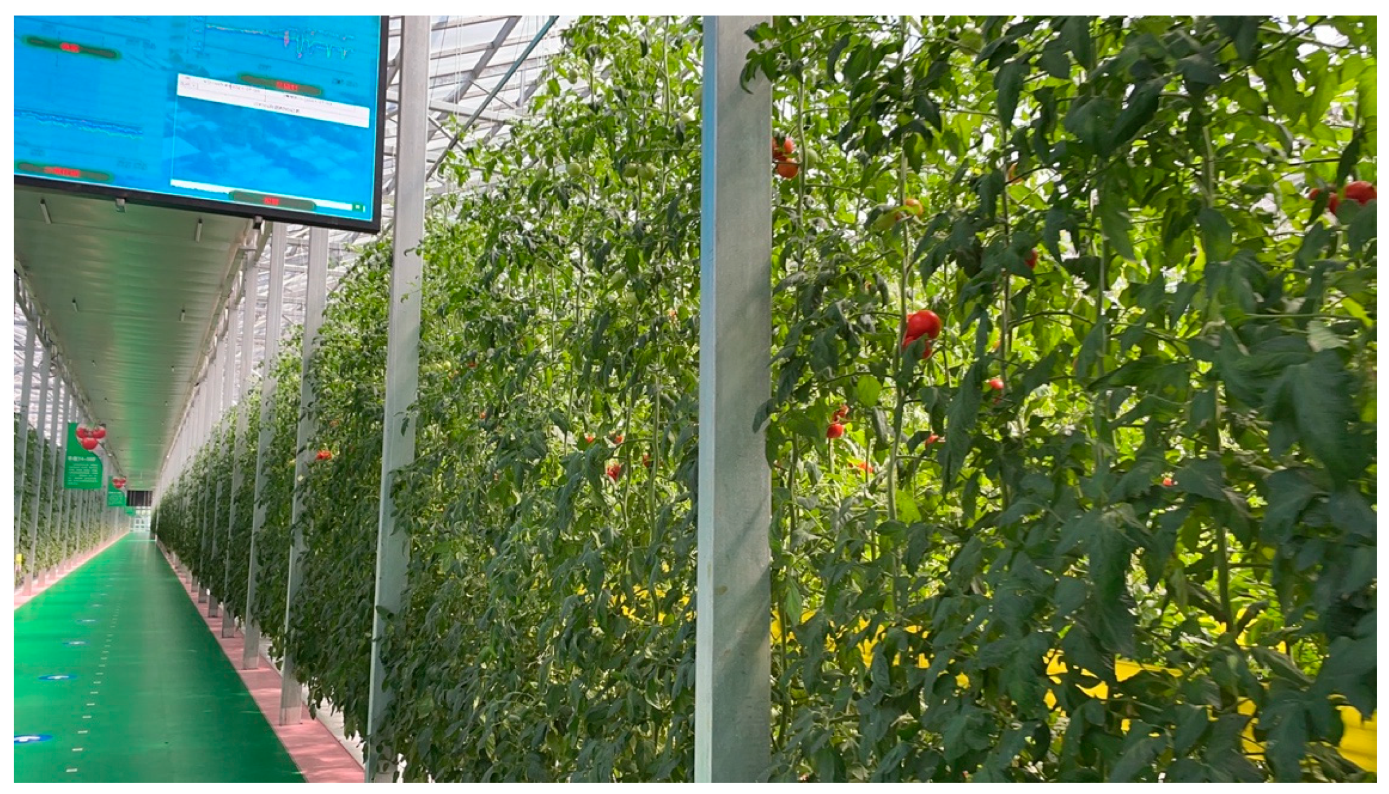
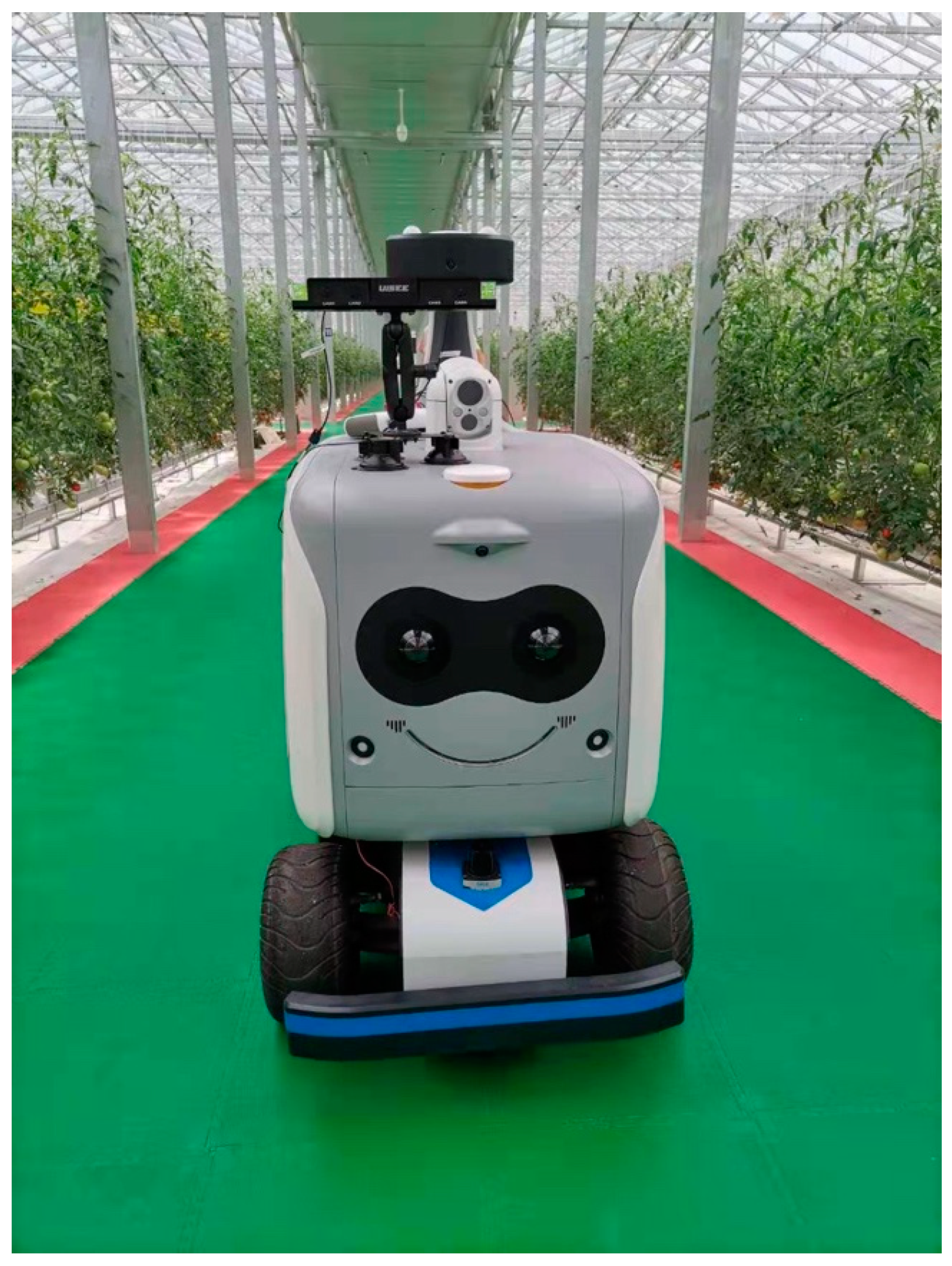
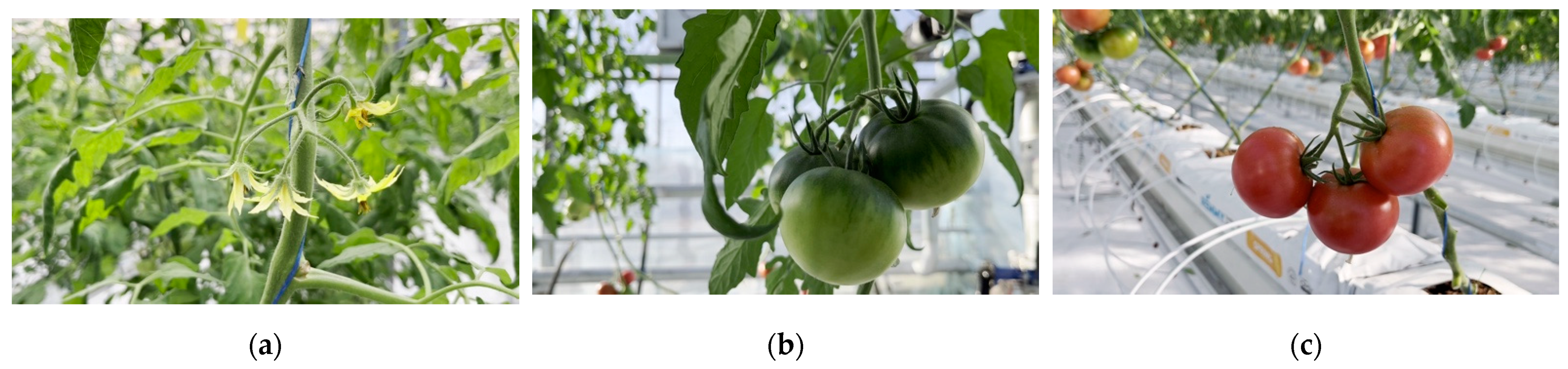
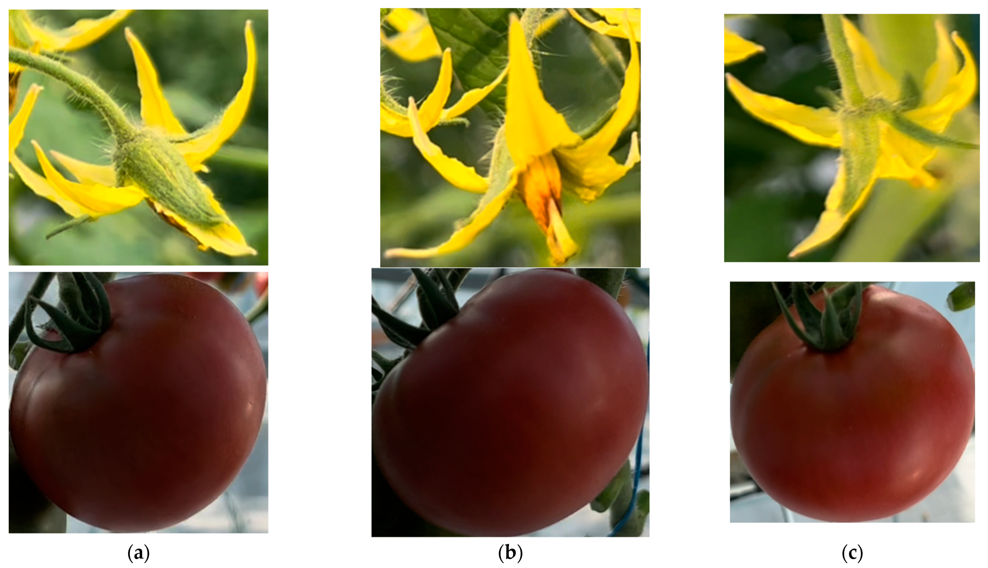
2.1.1. Data Acquisition and Experimental Environment

As shown in Figure 1, the collection of the experimental samples and the model effect test in this paper were all carried out in the National Vegetable Quality Standard Center (Shouguang, Shandong) Science and Technology Demonstration and Promotion Base. We set up the experiment in the greenhouse to ensure the engineering applicability of the algorithm. For the plant growth state data, the camera mounted on the inspection robot is used to obtain it. The inspection robot uses QR code navigation to conduct inspections through preset routes, as shown in Figure 2.

For video stream data, we intercept the images from the video stream every 10 fps to obtain images for training and testing of the object detection model. In this study, we divided the dataset into the training set and test set according to the ratio of 10:1, with 1000 training images and 100 testing images. As shown in Figure 3, we divide the targets into three categories: flower, tomato red, and tomato green, according to the needs of the actual production process. When we conducted a feasibility analysis at the beginning of the study, we found that the network had a low detection ability for tomato flowers and green tomatoes. Taking YOLOv5 s as an example, when the number of three types of targets in the training set is about 600, the mAP (0.95) of tomato flower, green tomato, and red tomato is 60.4%, 87.6%, and 94.3%, respectively. So, it is difficult for the network to distinguish the two types of objects of tomato flower and green tomato from the background in complex environments. Therefore, to improve the network’s high and balanced accuracy for these three objects, we artificially increase the number of tomato flowers and green tomatoes. The number of targets for each category is shown in

Table 1. The number of targets for each category.

Dataset	Flower	Tomato_Red	Tomato_Green	Total
Train set	1640	669	1138	3447
Test set	164	68	139	371

.

To realize the labeling of images, we use labelImg to label the objects in the photos. The effect after labeling is shown in Figure 4.

In addition, for the data set of the network in the target tracking part [29,30], we name it Tracking_tomato_115. The inspection robot collects the video at a constant speed. We use three camera positions to shoot the target, and each camera position captures one image every 10 fps for one target, and a total of five shots are captured. We collected and finally screened a total of 115 tomato and flower targets, and 1711 detected rectangles. At least two cameras capture each target, as shown in Figure 5.

2.1.2. Data Augmentation

Data augmentation is the most important way to improve model performance by artificially introducing prior knowledge into training data [31]. Since the samples obtained after enhancement strongly correlate with the original samples, the network is forced to learn various potential sample transformation methods. This study uses multiple data augmentation methods on the training set of the network’s object detection dataset to improve the robustness of the model in greenhouse scenes [16]. In addition, the images in the dataset are basically taken in the same scene, and the related data augmentation method can prevent the model from learning information irrelevant to the target and avoid overfitting. At the same time, data augmentation can also make up for the lack of data volume. For deep learning methods, whether the amount of data is sufficient will directly determine the effectiveness of the network. The specific approach and its parameter settings are as follows:

• The color gamut change is to generate a new image by randomly adjusting the original image’s color saturation, brightness, and contrast. The random adjustment of the input image color is vital for improving the robustness of the network and enhancing the model’s performance in complex greenhouse scenes. The image data’s HSV (Hue, Saturation, Value) describes the image’s color gamut distortion. The values of these three parameters are, respectively, Hue (h) is 0.015, Saturation (s) is 0.6, and the brightness (v) is 0.4.
• Flip the image from left to right in the horizontal direction, and each image has a 50% probability of flipping. This data enhancement method can also effectively expand the data volume of training samples.
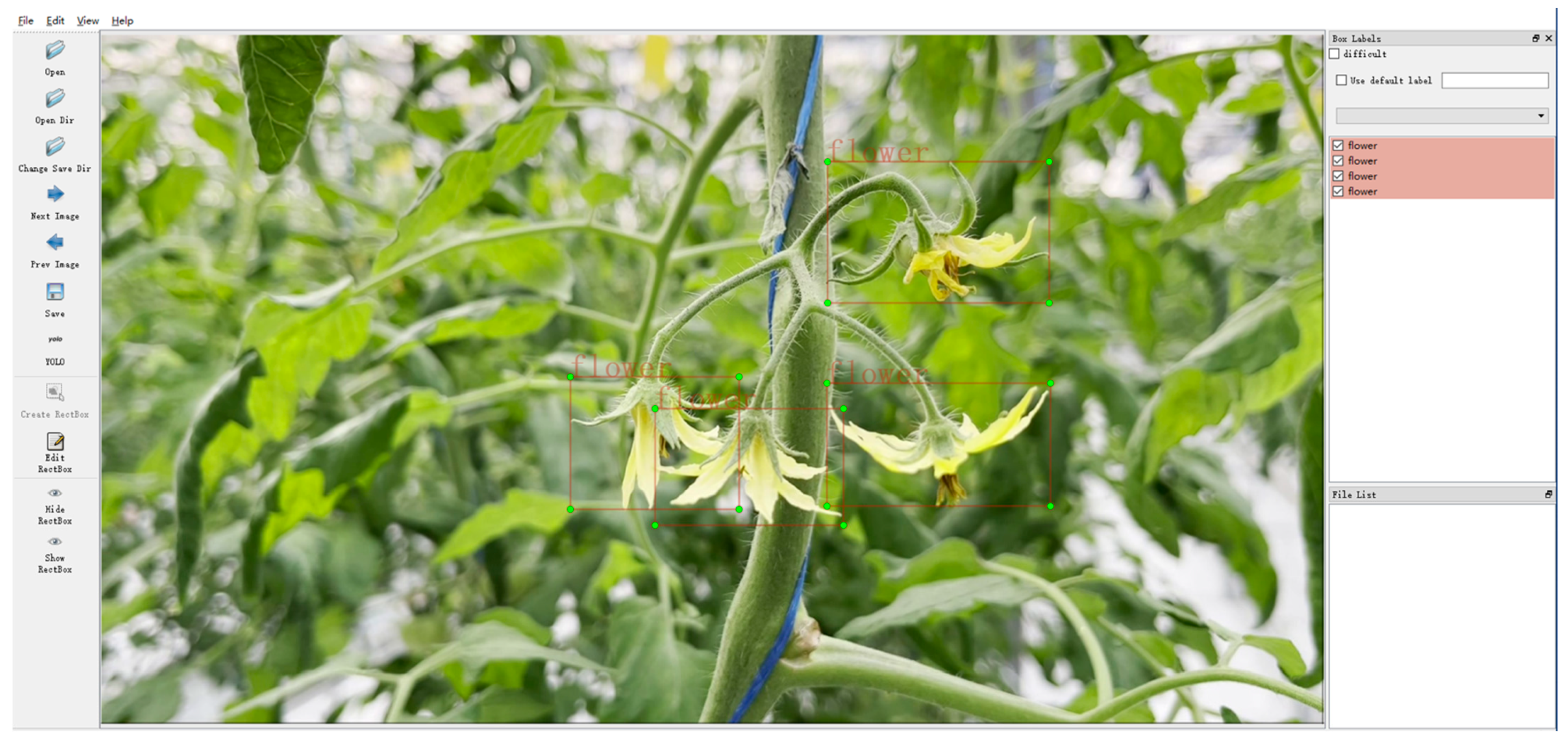
• To enhance the network’s ability to detect tomato flowers, we use mosaic enhancement technology and stitch the four images processed by steps 1 and 2 above by random scaling, random cropping, and random distribution. There are 4 different images are mixed, while CutMix mixes only 2 images [32]. This method effectively increases the diversity of images for the training process to improve the model’s ability to detect the flowers. And this method also effectively increases the number of images. Not only that, by splicing four images to form one, the batch size is increased in disguise, which reduces the GPU memory requirements for model training.

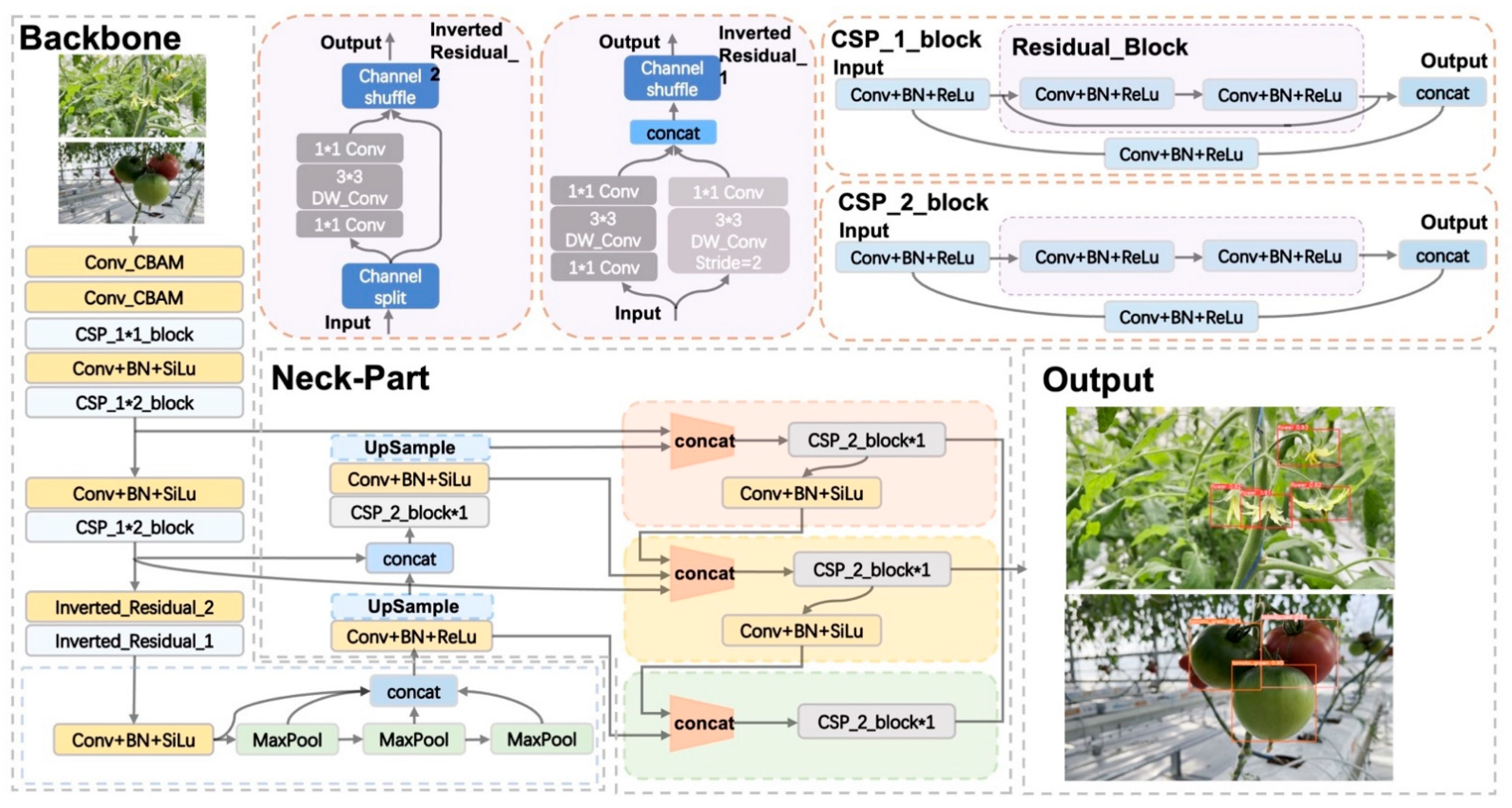
2.2. YOLO-Deepsort Model

2.2.1. Object Detection Model

This study proposes a new backbone for feature extraction of the object detection network based on YOLOv5 s. This research uses the Shufflenetv2 module to reuse and blend image features. The Shufflenetv2 module effectively reduces the complexity of the model [33]. We also use a convolutional module with a CBAM attention mechanism to minimize the impact of model feature extraction capability degradation caused by model lightweight [24]. Meanwhile, we use the bi-directional feature pyramid network (BiFPN) structure in the Neck part, which improves the ability of the network to utilize features [34]. The network structure is shown in Figure 6, and the network Parameters are shown in

Table 2. The parameters of YOLO-deepsort.

	From	n	Params	Module	Arguments
0	−1	1	3746	Conv_CBAM	[3, 32, 6, 2, 2]
1	−1	1	19,170	Conv_CBAM	[32, 64, 3, 2]
2	−1	1	18,816	CSP_1*1_block	[64, 64, 1]
3	−1	1	73,984	Conv + BN + SiLu	[64, 128, 3, 2]
4	−1	2	115,712	CSP_1*1_block	[128, 128, 2]
5	−1	1	295,424	Conv + BN + SiLu	[128, 256, 3, 2]
6	−1	3	625,152	CSP_1*1_block	[256, 256, 3]
7	−1	1	203,776	Inverted_Residual_2	[256, 512, 2]
8	−1	1	134,912	Inverted_Residual_1	[512, 512, 1]
9	−1	1	656,896	SPPF	[512, 512, 5]
10	−1	1	131,584	Conv + BN + SiLu	[512, 256, 1, 1]
11	−1	1	0	Upsample
12	[−1, 6]	1	0	Concat	[1]
13	−1	1	361,984	CSP_2*1_block	[512, 256, 1]
14	−1	1	33,024	Conv + BN + SiLu	[256, 128, 1, 1]
15	−1	1	0	Upsample
16	[−1, 6, 14]	1	0	Concat	[1]
17	−1	1	90,880	CSP_2*1_block	[256, 128, 1]
18	−1	1	147,712	Conv + BN + SiLu	[128, 128, 3, 2]
19	[−1, 6, 14]	1	0	Concat	[1]
20	−1	1	361,984	CSP_2*1_block	[512, 256, 1]
21	−1	1	590,336	Conv + BN + SiLu	[256, 256, 3, 2]
22	[−1, 10]	1	0	Concat	[1]
23	−1	1	1,182,720	CSP_2*1_block	[512, 512, 1]
24	[17, 20, 23]	1	21,576	Detect

.

From the table, we can see that the object detection model proposed in this study consists of the following four parts in total:

4.

Inherited from the CSP-1-block of the original YOLOv5’s backbone, this hierarchical feature fusion mechanism of the CSP structure effectively strengthens the learning ability of the convolutional neural network. It reduces the number of parameters of the network. Using the CSP structure can effectively alleviate the problem of gradient disappearance. In addition, the CSP structure is nested by multiple residual structures [35]. The basic module in the residual structure is CBL (convolution, batch normalization, SiLu).

5.

The SPPF structure is used to replace the SPP (spatial pyramid pooling) structure as the output of the last layer of the backbone [36]. The feature map level fusion of local and global features is achieved through the SPPF module. In addition, the SPPF structure dramatically improves the speed of network operations and the feature information-carrying capacity of feature maps.

6.

The feature vector extracted by the shallow network often contains rich location information, such as contours and texture information. In contrast, the feature vectors extracted by deep feature extraction networks often contain rich semantic information and less location information. The location information determines the prediction accuracy of the target location, and the semantic information determines the accuracy of the target category prediction. Our model uses BiFPN [34] as the Neck-Part of the network to maximize the use of the feature information.

7.

The Head Part is used for the final detection part, applying anchor boxes on the feature map and generating regression parameters with class probability, target probability score, and bounding box [15]. YOLO-deepsort has a total of three heads. The scales of these heads are (80 × 80 × 21) (40 × 40 × 21) (20 × 20 × 21), each head has a total of (classes + confidence + coordinate offsets (dx, dy, dw, dh)) × 3 anchor boxes, a total of 21 channels.

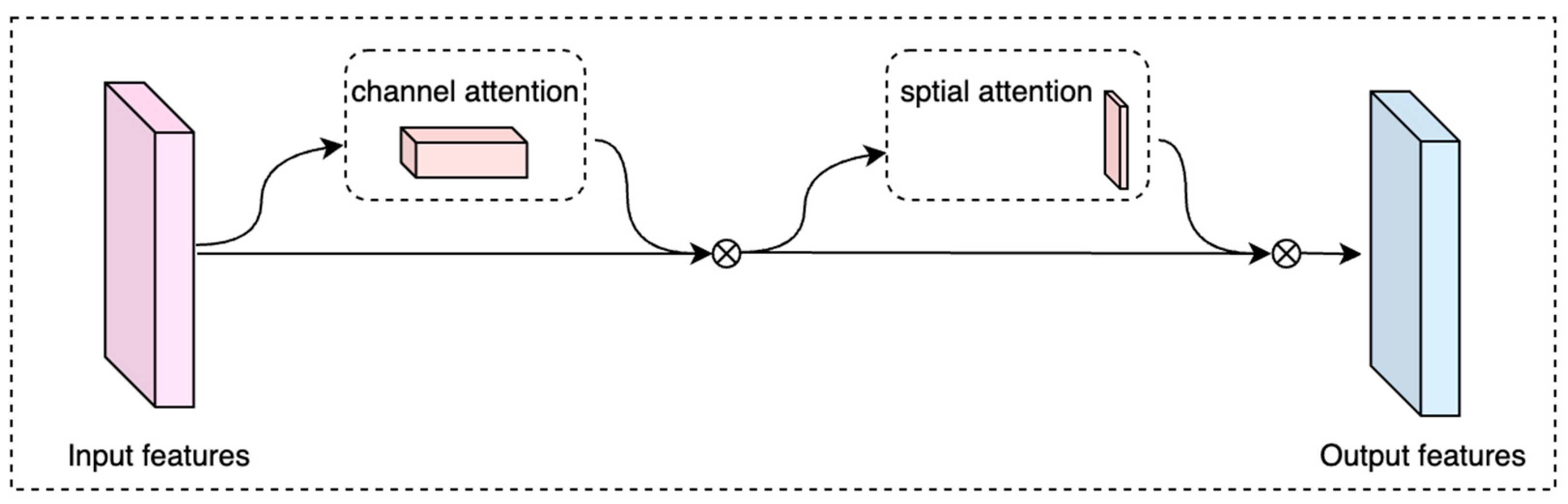
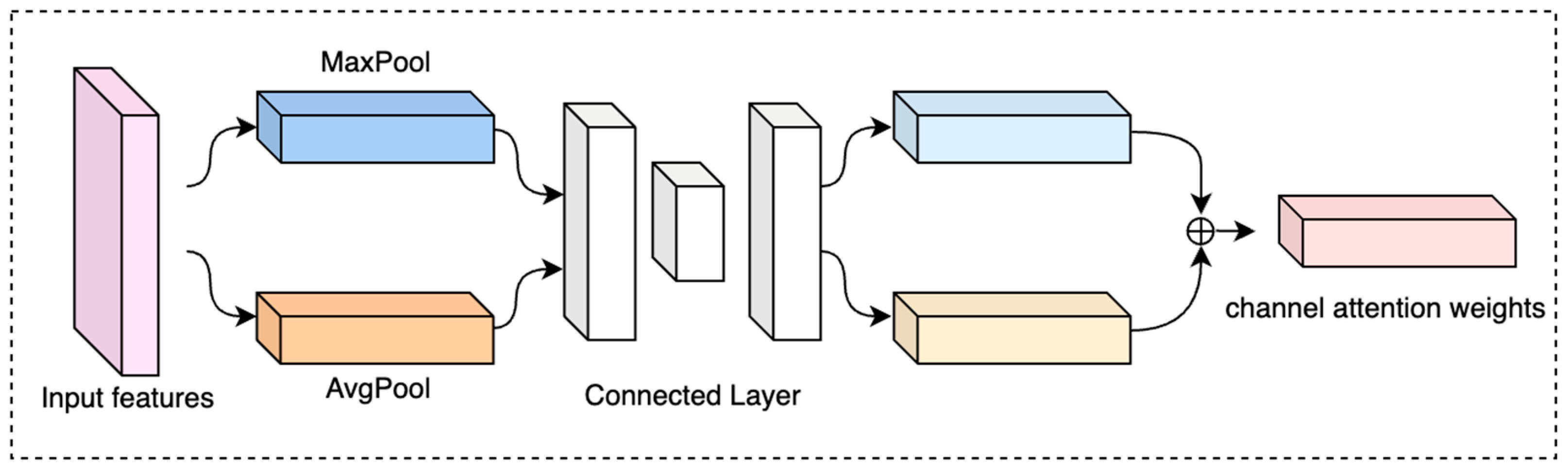
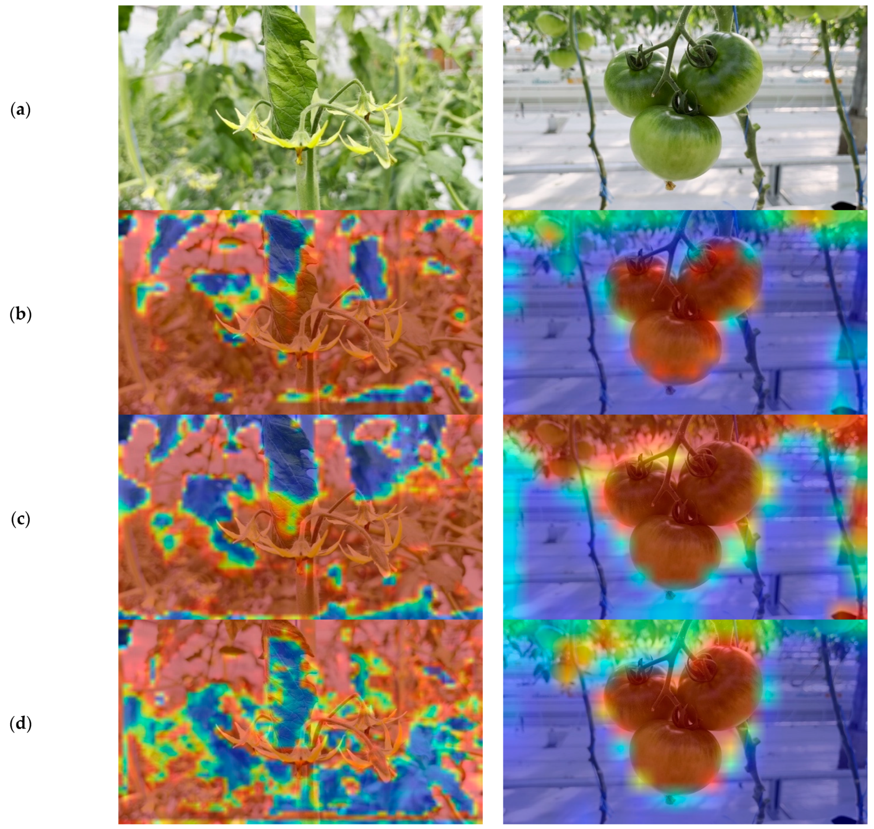
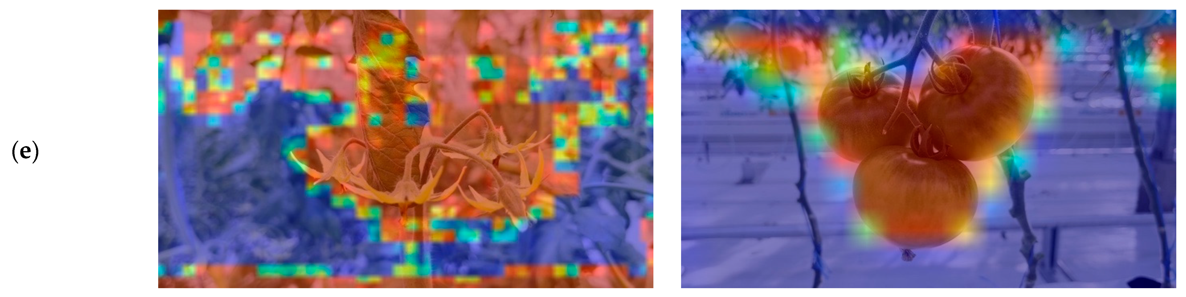
2.2.2. Attention Module

CBAM (Convolutional Block Attention Module) is an attention mechanism module that merges spatial and channel attention [24], as it is shown in Figure 7.

First, the CBAM attention mechanism performs global average pooling and global max pooling on the feature map, the processed output feature matrix sizes are (1 × 1 × channels) and (1 × 1 × channels), respectively. Then, the two groups of channel weights are combined after passing through the fully connected layer, and then the weights in the channel dimension are obtained through the non-linear activation layer [23], as shown in Figure 8.

Secondly, the feature matrix obtained after the input feature matrix is weighted by the channels, as mentioned above, also uses global pooling and average pooling to process the channel dimension of the feature matrix. The resulting output feature matrix shapes are (h × w × 1) (h × w × 1). Finally, through the convolution layer with a kernel size of 7, the output feature matrix of size (h × w × 1) is obtained through the convolution and non-linear activation layer processing, as shown in Figure 9.

The purpose of adding the CBAM attention mechanism in this study is to eliminate the loss of model feature extraction capability caused by using the lightweight module.

2.2.3. Lightweight Module

Shufflenetv2 is a lightweight model based on principles of efficient CNN network design. To improve the defects of shufflenetV1 [37], shufflenetV2 introduces a new operation called channel split [23]. Figure 10a shows that the input feature map will be equally divided into two branches in the channel dimension. The left branch is equally mapped, the right branch contains three convolutions, and the input and output channels are the same. The two branches are spliced together after completing the operations, respectively. The network uses a channel shuffle to reorganize the spliced output to ensure the information exchange between the two branches above. As shown in Figure 10b, there is no additional channel split for the down sampling module, but each branch directly copies an input, and each branch has down sampling with a stride is 2. Finally, after stitching these two branches together, the feature map space size is halved, and the number of channels is doubled.

2.2.4. BiFPN Module

The difficulty in improving the performance of the target detection network is the effective representation and processing of multi-scale features. Feature Pyramid Networks (FPN), a seminal work in this section, proposes a top-down approach to combining multi-scale features [38]. Based on FPN, a new FPN structure called Path Aggregation Network (PANet) for Instance Segmentation that strengthens the bottom-up path is proposed, which improves the utilization efficiency of features of different network layers [39]. To improve the ability of the model to detect objects of different scales, bi-directional feature pyramid network (BiFPN) adopts the idea of bidirectional cross-scale connection and weighted feature fusion to fuse more features without increasing the cost [34]. The BiFPN structure performs a series of mixing and combining image features and passes the image features to the prediction layer. Figure 11 shows three different compound scaling methods.

2.2.5. DeepSort Model

The predecessor of Deepsort was SORT (sample online and real-time tracking) [29]. As a cascade matching algorithm, the network takes the detection result as input (bounding box, confidence, feature), where confidence is mainly used to filter the bounding box, and the bounding box and feature match the target with the tracker calculated later. The Deepsort algorithm uses a Kalman filtering algorithm to generate a tracker based on the target in the previous frame [40]. The Kalman filter algorithm is divided into two processes, prediction, and update.

8.

Prediction: When the target passes through a building, parameters such as the target frame position and speed of the current frame are predicted through parameters such as the target frame and speed of the previous frame.

9.

Update: The predicted and observed values, the two states of the normal distribution, are linearly weighted to obtain the state predicted by the current system.

We obtain the corresponding targets in the target box and perform feature extraction on these targets using a deep neural network. Then the similarity calculation is performed on the trajectory and appearance features of the target and the tracker. For the trajectory matching calculation, the model uses the Mahalanobis distance Equation (1) to measure the differences between the tracker and the target [41].

$$t^{\left(1\right)}\left(i,j\right)={\left(t_j-y_i\right)}^T{S}_i^{-1}\left(t_j-y_i\right)$$

(1)

where $t_j$ represents the target $j$, $y_i$ represents tracker $i$ and $S_i^l$ represents the covariance of $t$ and $y$. The model measures the similarity between the target and the tracker by the cosine distance Equation (2).

$$t^{\left(2\right)}\left(i,j\right)=\underset{ }{\min }\{1-r_j^T{r}_k^{\left(i\right)}|r_k^{\left(i\right)}ϵR_i\}$$

(2)

where $1-r_j^T{r}_k^{\left(i\right)}$ represents cosine distance. The cosine distance is used to measure the apparent features of the track and the apparent features corresponding to the detection to predict the ID more accurately. Combining Equations (1) and (2), the comprehensive matching degree formula of the model is obtained.

$$c_{i,j}=\lambda t^{\left(1\right)}\left(i,j\right)+\left(1-\lambda \right)t^{\left(2\right)}\left(i,j\right)$$

(3)

After the model mentioned above similarity calculation, the model also constructs a similarity matrix by calculating the IoU of the tracker and the target, and finally obtains the cost matrix. The Hungarian algorithm matches the predicted tracker with the target in the current frame [42]. Finally, the parameters of the Kalman filter are updated according to the matching results. Figure 12 shows the flowchart of the Deepsort algorithm.

2.3. Evaluation of Model Performance

In this study, the following metrics are implemented to evaluate the model’s performance: precision, recall, F1 score, and mAP (Mean Average Precision). The first letter represents the correctness of this prediction, T is true, and F is False; the second letter represents the category predicted by the classifier, P represents the positive samples predicted, and N represents the negative samples predicted. Our study uses mean accuracy (mAP) to measure the model performance. The meanings of the relevant parameters and the consensus are as follows:

• TP(True Positive): the prediction result and ground truth are positive samples
• FP(False Positive): the detection result is negative, but the prediction result is true
• TN(True Negative): the prediction result and ground truth are both negative samples
• FN(False Negative): the detection result is positive instead of negative

The calculation function is as follows:

$$Precision=\frac{TP}{TP+FP}\ast 100\%$$

(4)

$$Recall=\frac{TP}{TP+FN}\ast 100\%$$

(5)

$$F{1}_{score}=\frac{2\ast Precision\ast Recall}{Precision+Recall}$$

(6)

$$mA{P}_{0.95}=\frac{1}{2}{\displaystyle \sum }_{m=0}^1{{\displaystyle \int }}_0^1{P}_m\left(R_m\right)d{R}_m\ast 100\%$$

(7)

3. Results

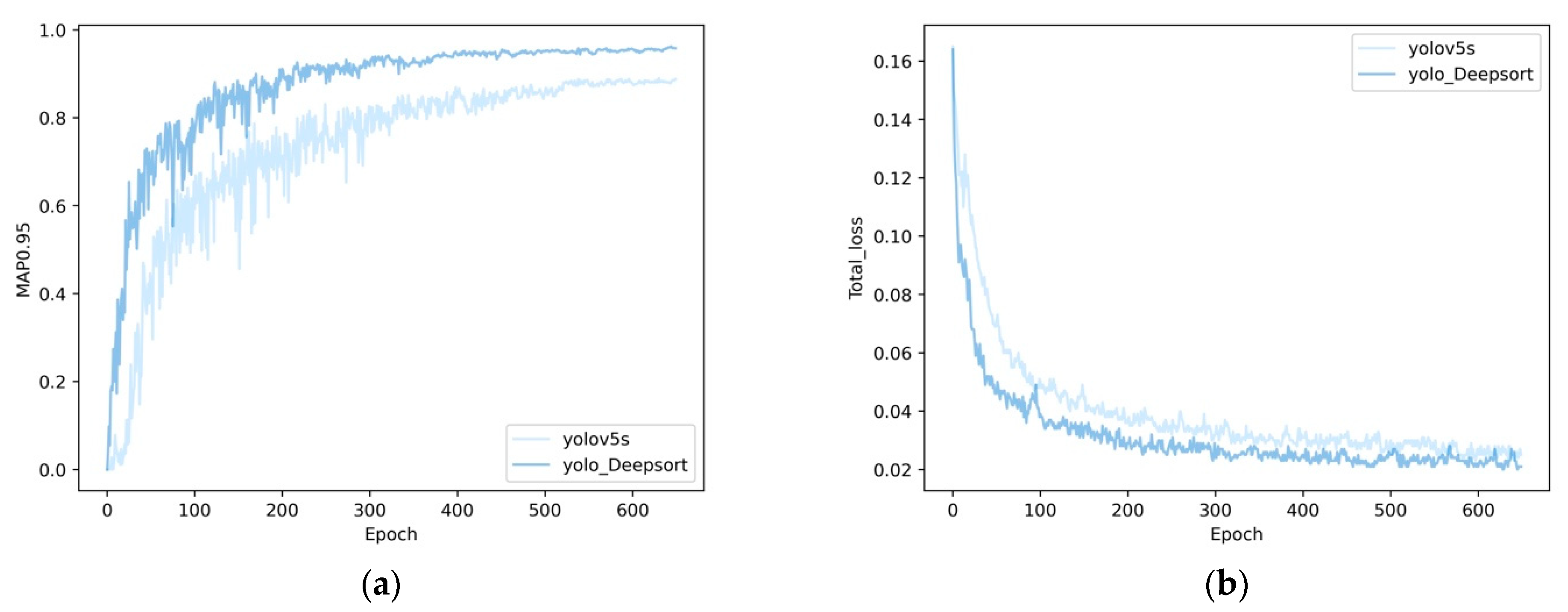
3.1. Object Detection Part Training

For model training, the setting of hyperparameters significantly impacts the model’s training effect. Unlike model parameters, hyperparameters do not depend on data to dynamically change but are manually adjusted parameters before or during training. Among them, the design and debugging of the model’s optimization parameters and regularization parameters, such as learning rate, batch size, optimizer, and weight decay, will directly or indirectly impact the final effect of the network. The purpose of the optimization and adjustment of the network model is to find the optimal global solution, and the regular term hopes that the model will fit as best as possible. Model optimization seeks to minimize empirical risk, making it easy to fall into overfitting. The regular term is used to constrain model complexity. So how to balance the relationship between the two and get the optimal solution is the purpose of hyperparameter adjustment. The results often confirm that the appropriate setting of hyperparameters is more critical than other methods for improving network performance.

Table 3. The appropriate values for some hyperparameters and the effect of this hyperparameter setting on model performance.

Hyperparameter	Selection	Notice
learning rate	SGD [43]	If the learning rate is too high or too low, the optimization of the model will fail.
momentum	0.937	Speed up convergence, jump out of the extreme point and avoid falling into the local optimal solution
weight_decay	0.0005	Constrain the number of parameters, prevent model overfitting
batch size	8	Updating the weight every 8 images per iteration
box	0.05	In most cases, the loss function hyperparameters may affect the optimization. Inappropriate hyperparameters will make it challenging to optimize the model even if the loss function is very suitable for the target optimization.
cls	0.5
cls_pw	1.0
obj	1.0
obj_pw	1.0
Iou_t	0.2
anchor_t	4.0

box: box loss gain; cls: cls loss gain; cls_pw: cls BCELoss positive_weight; obj: obj loss gain (scale with pixels); obj_pw: obj BCELoss positive_weight; IoU_t: IoU training threshold; anchor_t: anchor-multiple thresholds.

shows the setting range of hyperparameters in this study. The selection of hyperparameters in this study is based on our subjective judgments based on practice and previous experience, which can be further discussed. Moreover, to reduce overfitting, after each iteration of 16 images, the network is evaluated on a validation set of 100.

At the same time, we use the warm-up method to warm up the learning rate when the learning rate is updated. The warm-up stage uses a one-dimensional linear interpolation method to update the learning rate of each iteration. When the warm-up phase is complete, the model uses the cosine annealing algorithm Equation (8) to update the learning rate during the rest of the training process.

$$ne{w}_{lr}=l{r}_{min}+\left(l{r}_{init}-l{r}_{min}\right)\ast ((1+\cos (\frac{cu{r}_{epoch}}{tota{l}_{epoch}}\ast \pi ))/2)$$

(8)

In addition, YOLO-deepsort uses different learning rate adjustment methods for different layers, including the weight layer, bias layer, and BN layer [9]. This strategy can make the training process more efficient. To reduce the number of repeated boxes, we use non-maxima suppression (NMS) and set a threshold of 0.5. By calculating the overlap between the output box and the bounding box by CIoU Equation (9), the bounding box that exceeds the threshold will be filtered out. Therefore, when the threshold is set higher, the number of bounding boxes predicted by the network will decrease, and vice versa, the number of boxes inference by the network will increase.

$$CIoU=IoU-\left(\frac{{\rho }^2\left(b,b^{gt}\right)}{c^2}+\alpha v\right)$$

(9)

$$v=\frac{4}{{\pi }^2}{\left(arctan\frac{w^{gt}}{h^{gt}}-arctan\frac{w}{h}\right)}^2$$

(10)

$$\alpha =\frac{v}{\left(1-IoU\right)+v}$$

(11)

where $b$ represents the parameters of the predicted box center coordinates, and $b^{gt}$ represents the parameters of the center of the object bounding box. $p^2$ is the square of the distance between the two center points, and the layer represents the diagonal length of the minimum circumscribed rectangle of the two rectangles. $\alpha$ and $\nu$ are aspect ratios, and $w$,$h$, $w^{gt}$, and $h^{gt}$ represent the height of the predicted box and the height and width of the bounding box, respectively.

3.2. Object Detection Part Result

The detection algorithm of the YOLO_deepsort model is improved based on the YOLOv5 s model. We compare the training process between the YOLOv5 s model and our method to show the algorithm’s performance, as shown in Figure 13.

Figure 13a shows the model’s mean average precision change during the training process. For the target detection network, the higher the mAP(0.95), the better the detection effect of the model. As we can see, the speed of YOLO_deepsort model’s mean average precision improvement within 100 epochs is better than that of YOLOv5 s with minor fluctuation. In addition, the mAP(0.95) of the improved YOLO_deepsort model gradually stabilizes after 350 epochs, while the YOLOv5 s model does not gradually stabilize until the mAP of the 500-epoch model. The loss function curve of the model is often used to evaluate the model’s performance. As shown in Figure 13b, the loss function curve of the improved YOLO_deepsort model converges faster in the first 100 epochs than the YOLOv5 s model. The total loss of the improved YOLO_deepsort model is a little lower than that of YOLOv5 s.

3.3. Object Tracking Part

The target tracking network uses deep learning methods to extract target features to help the target tracking network detect and match the bounding box of the network with the tracker. Therefore, before online tracking, we first train a convolutional neural network offline for feature extraction of the tracked target. We used a computer configured with an Intel Core Xeon(R) CPU 2.5 GHz, 64 GB running memory, and 12 GB Nvidia GTX 2080 Ti GPU to implement the above convolutional neural network training, CUDA version 10.1 parallel computing architecture, and cuDNN version 7.6 network Acceleration library. The operating environment is Ubuntu 20.04 and PyTorch3.0. The training process of CNN is shown in Figure 14; we train the CNN offline for over 3500 epochs. Figure 14a shows that the loss on the test set is close to optimal when it exceeds 2000 epochs. The loss function evaluates the model by measuring the error between the prediction and true values. In Figure 14b, the top1 loss of the model gradually decreasing means that even if the shooting angle of the target changes, the model can still judge whether it is the same target according to its characteristics. The target features extracted by the CNN network will be used as an essential basis for matching the bounding box and the tracker, contributing to improving target tracking accuracy.

4. Discussion

4.1. Comparison with Other Object Detection Methods

To illustrate the performance of the YOLO-deepsort model, we compare the model with YOLOv5 s, YOLOv5 m, and YOLOv5 l. The above method is trained with the same dataset and device, and then the object detection models are compared using the same test set.

Table 4. The detection results of a series of YOLO networks and YOLO-deepsort.

Model	Precision	Recall	F1-Score	mAP (0.5:0.95)	Parameters
YOLOv5 s	99.5%	90.6%	94.8%	88.7%	7,018,216
YOLOv5 m	99.5%	95.3%	97.4%	91.6%	13,354,682
YOLOv5 l	99.5%	94.1%	96.7%	91.6%	46,119,048
YOLO-deepsort	99.5%	98.4%	98.9%	95.8%	5,072,848

shows that YOLO-deepsort has high precision, recall, and mAP (mean average precision) in the detection tasks of different growth stages of tomato (flowering stage, unripe fruit, ripe fruit). By comparing the metrics in the table, we can see that our model has better performance than other YOLO series object detection networks. Specifically, compared with YOLOv5 s, the precision of YOLO-deepsort remains unchanged, the F1-score is improved by 4.1%, and the mAP (0.95) is improved by 7.1%. The YOLO-deepsort model has fewer parameters and is very friendly to model deployment, which meets the requirements for the greenhouse inspection robot to count tomato flowers during travel and provides conditions for the network to follow up on target tracking. In general, YOLO-deepsort model can meet the requirements for real-time monitoring in the greenhouse.

To illustrate the high performance of our method, we drew a heatmap of the above model, and YOLO-deepsort with different methods added, as shown in Figure 15. The above results and visual heat map prove that YOLO-deepsort can fulfill the detection of different periods of tomato and meet the requirements of practical application deployment. In Figure 15, we show the heatmap of different networks, further demonstrating our approach’s performance. By setting the target confidence to 0.75 (Filter out targets with probability scores below 75% to prevent the model from detecting distant targets and causing double counting), the model can only detect the target of the current row during the inference process to avoid double-counting. We can see that the detection capabilities of different models for the tomatoes are similar. However, for flower recognition, the area of interest of YOLO-deepsort is more concentrated in the area where the target is located, showing a strong detection ability.

4.2. Comparison with Other Object Lightweight Methods

Complex models often have better performance, but high storage space and computing resource consumption are difficult to apply. Therefore, in the model design process, we tried to reduce the consumption of the model’s computing memory and realized the compression of the model from the algorithm level.

Table 5. The storage cost of YOLO-deepsort and other lightweight models.

Model	Input_Size	Params	Size(M)	Percision	mAP(0.5:0.95)
YOLO_nano	416 × 416	-	34.8	30.5%	15.4%
YOLOv3-tiny	416 × 416	8.67 M	17.4	95.7%	86.7%
YOLOv5 n	640 × 640	1.76 M	3.8	96.7%	85.4%
YOLOv5_Lite	640 × 640	5.39 M	10.9	99.2%	91.3%
YOLO-deepsort	640 × 640	5.07 M	10.5	99.5%	95.8%

shows the model size, parameter quantity, and model performance of YOLO-deepsort and various existing lightweight models. For scenes where the relationship between the background and the subject is relatively stable, the existing lightweight network will have better results, but it is not easy to achieve the expected results in complex agricultural scenes. The number of model parameters of YOLO-deepsort is only 5.07(Million), the size of the weight file is only 10.5 MB, and the detection part of the network of YOLO-deepsort can still achieve target recognition and detection well in agricultural scenarios.

4.3. Performance of Object Tracking and Counting

Our method achieves the function of tracking and counting tomato flowers in complex agricultural scenarios. We calculate the objects that hit the line by setting a virtual counting statistic line. Due to the complexity of crop growth in the actual scene, it is difficult for us to ensure that the camera will not repeatedly collect the target. Our research is based on the realization of target tracking to complete the counting task. The algorithm itself can identify the target in the current video stream, which means that when the same target repeatedly hits the line, it will not be a repeated count. The counting process is shown in Figure 16.

The three targets in the images are each assigned a specific ID, and the ID of each target is still maintained while the camera position is constantly moving. In the greenhouse environment, the land is uneven, and the inspection robot equipped with a camera has poor shooting stability during the inspection process. The instability of the video data can easily lead to the missed detection of the target in some frames. In response to the above situation, YOLO-deepsort will store the characteristics of the target whose id was previously determined to ensure that the id of the target does not change when the target is successfully detected next time.

5. Conclusions

In recent years, given the practical application needs of target detection and yield prediction in facility agriculture, we propose a tomato counting method based on an object tracking algorithm and apply it to tomato yield prediction. Overall, the contributions of this paper are as follows.

To realize the detection and counting of tomatoes at different growth stages, we propose an improved YOLO model and combine it with the target tracking algorithm using a deep feature extraction network. In addition, to collecting and labeling images of tomatoes at different growth stages for training the object detection network, we also collected a dataset called Tracking_tomato_115 for training the object tracking network. For the model object detection part of the network, we embedded the lightweight structure and CBAM module into the backbone network and used the BiFPN structure at the neck of the model. During the training process, warm-up and cosine annealing algorithms are used to update the learning rate of the model. Then, we use Deepsort to achieve object tracking of tomato fruits and flowers. We use the YOLO-deepsort model to test in a greenhouse environment. The experimental results show that our algorithm can effectively avoid the occurrence of double counting and achieve good practical results. After getting the tracking results, we use OpenCV to create a virtual count line to count the targets. Compared with the original YOLOv5 s model, our method achieved a competitive result. The mean average precision of flower, green tomato, and red tomato was 93.1%, 96.4%, and 97.9%, which increased by 17%, 2%, and 2.3%, respectively. Also, our model weights are only 10.5 MB, and the memory consumption is lower than most lightweight networks under the premise of ensuring performance. Our model meets the requirements for the greenhouse inspection robot to count tomato flowers during travel and provides conditions for the network to follow up on target tracking.

However, the detection is unstable due to the complex environment of the greenhouse and the shaking during the inspection process, which will adversely affect the target tracking and counting. In the future, we will continue improving the model’s speed and stability for real-time detection in complex scenes.

References

1. Zhou, L.; Song, L.; Xie, C.; Zhang, J. Applications of Internet of Things in the Facility Agriculture. In Computer and Computing Technologies in Agriculture VI. CCTA 2012. IFIP Advances in Information and Communication Technology; Li, D., Chen, Y., Eds.; Springer: Berlin/Heidelberg, Germany, 2013; Volume 392. [Google Scholar] [CrossRef] [Green Version]
2. Jin, X.-B.; Yu, X.-H.; Wang, X.-Y.; Bai, Y.-T.; Su, T.-L.; Kong, J.-L. Deep Learning Predictor for Sustainable Precision Agriculture Based on Internet of Things System. Sustainability 2020, 12, 1433. [Google Scholar] [CrossRef] [Green Version]
3. Yin, H.; Chai, Y.; Yang, S.X.; Mittal, G.S. Ripe Tomato Recognition and Localization for a Tomato Harvesting Robotic System. In Proceedings of the 2009 International Conference of Soft Computing and Pattern Recognition, Washington, DC, USA, 4–7 December 2009; pp. 557–562. [Google Scholar] [CrossRef]
4. Suykens, J.; Vandewalle, J. Least Squares Support Vector Machine Classifiers. Neural Process. Lett. 1999, 9, 293–300. [Google Scholar] [CrossRef]
5. Liu, G.; Mao, S.; Kim, J.H. A Mature-Tomato Detection Algorithm Using Machine Learning and Color Analysis. Sensors 2019, 19, 2023. [Google Scholar] [CrossRef] [PubMed] [Green Version]
6. Amarante, M.A.; Ang, A.; Garcia, R.; Garcia, R.G.; Martin, E.M.; Valiente, L.F.; Valiente, L., Jr.; Vigila, S. Determination of Ripening Stages and Nutritional Content of Tomatoes Using Color Space Conversion Algorithm, Processed Through Raspberry Pi. In Proceedings of the International Conference on Biomedical Engineering and Technology, Tokyo, Japan, 15–18 September 2020. [Google Scholar] [CrossRef]
7. Simonyan, K.; Zisserman, A. Very deep convolutional networks for large-scale image recognition. In Proceedings of the International Conference on Learning Representations (ICLR), San Diego, CA, USA, 7–9 May 2015. [Google Scholar]
8. Szegedy, C.; Liu, W.; Jia, Y.; Sermanet, P.; Reed, S.; Anguelov, D.; Erhan, D.; Vanhoucke, V.; Rabinovich, A. Going deeper with convolutions. In Proceedings of the 2015 IEEE Conference on Computer Vision and Pattern Recognition (CVPR), Boston, MA, USA, 7–12 June 2015; pp. 1–9. [Google Scholar] [CrossRef] [Green Version]
9. He, K.; Zhang, X.; Ren, S.; Sun, J. Deep residual learning for image recognition. In Proceedings of the IEEE Conference on Computer Vision and Pattern Recognition (CVPR), Las Vegas, NV, USA, 27–30 June 2016; pp. 770–778. [Google Scholar]
10. Girshick, R.; Donahue, J.; Darrell, T.; Malik, J. Rich feature hierarchies for accurate object detection and semantic segmentation. In Proceedings of the IEEE Conference on Computer Vision and Pattern Recognition, Columbus, OH, USA, 23–28 June 2014; pp. 580–587. [Google Scholar]
11. Girshick, R. Fast r-cnn. In Proceedings of the IEEE International Conference on Computer Vision, Washington, DC, USA, 7–13 December 2015; pp. 1440–1448. [Google Scholar]
12. Ren, S.; He, K.; Girshick, R.; Sun, J. Faster R-CNN: Towards Real-Time Object Detection with Region Proposal Networks. IEEE Trans. Pattern Anal. Mach. 2022, 44, 154–180. [Google Scholar] [CrossRef] [PubMed] [Green Version]
13. Redmon, J.; Divvala, S.; Girshick, R.; Farhadi, A. You only look once: Unified, real-time object detection. In Proceedings of the IEEE conference on Computer Vision and Pattern Recognition, Las Vegas, NV, USA, 27–30 June 2016; pp. 779–788. [Google Scholar]
14. Redmon, J.; Farhadi, A. YOLO9000: Better, faster, stronger. In Proceedings of the IEEE Conference on Computer Vision and Pattern Recognition, Honolulu, HI, USA, 21–26 July 2017; pp. 7263–7271. [Google Scholar]
15. Redmon, J.; Farhadi, A. Yolov3: An incremental improvement. arXiv 2018, arXiv:1804.02767. [Google Scholar]
16. Bochkovskiy, A.; Wang, C.-Y.; Liao, H.-Y.M. Yolov4: Optimal speed and accuracy of object detection. arXiv 2020, arXiv:2004.10934. [Google Scholar]
17. Ko, K.; Jang, I.; Choi, J.H.; Lim, J.H.; Lee, D.U. Stochastic Decision Fusion of Convolutional Neural Networks for Tomato Ripeness Detection in Agricultural Sorting Systems. Sensors 2021, 21, 917. [Google Scholar] [CrossRef]
18. Seo, D.; Cho, B.-H.; Kim, K.-C. Development of Monitoring Robot System for Tomato Fruits in Hydroponic Greenhouses. Agronomy 2021, 11, 2211. [Google Scholar] [CrossRef]
19. Liu, G.; Nouaze, J.C.; Touko Mbouembe, P.L.; Kim, J.H. YOLO-Tomato: A Robust Algorithm for Tomato Detection Based on YOLOv3. Sensors 2020, 20, 2145. [Google Scholar] [CrossRef] [Green Version]
20. Magalhães, S.A.; Castro, L.; Moreira, G.; dos Santos, F.N.; Cunha, M.; Dias, J.; Moreira, A.P. Evaluating the Single-Shot MultiBox Detector and YOLO Deep Learning Models for the Detection of Tomatoes in a Greenhouse. Sensors 2021, 21, 3569. [Google Scholar] [CrossRef]
21. Sun, J.; He, X.; Ge, X.; Wu, X.; Shen, J.; Song, Y. Detection of Key Organs in Tomato Based on Deep Migration Learning in a Complex Background. Agriculture 2018, 8, 196. [Google Scholar] [CrossRef] [Green Version]
22. Dzmitry, B.; Kyunghyun, C.; Yoshua, B. Neural Machine Translation by Jointly Learning to Align and Translate. arXiv 2015, arXiv:1409.0473. [Google Scholar]
23. Hu, J.; Shen, L.; Sun, G. Squeeze-and-Excitation Networks. In Proceedings of the 2018 IEEE/CVF Conference on Computer Vision and Pattern Recognition, Salt Lake City, UT, USA, 18–22 June 2018; pp. 7132–7141. [Google Scholar]
24. Woo, S.; Park, J.; Lee, J.Y.; Kweon, I.S. CBAM: Convolutional block attention module. In Proceedings of the European Conference on Computer Vision (ECCV), Munich, Germany, 8–14 September 2018; pp. 3–19. [Google Scholar]
25. Chen, Z.; Wu, R.; Lin, Y.; Li, C.; Chen, S.; Yuan, Z.; Chen, S.; Zou, X. Plant Disease Recognition Model Based on Improved YOLOv5. Agronomy 2022, 12, 365. [Google Scholar] [CrossRef]
26. Yang, B.; Gao, Z.; Gao, Y.; Zhu, Y. Rapid Detection and Counting of Wheat Ears in the Field Using YOLOv4 with Attention Module. Agronomy 2021, 11, 1202. [Google Scholar] [CrossRef]
27. Lu, S.; Song, Z.; Chen, W.; Qian, T.; Zhang, Y.; Chen, M.; Li, G. Counting Dense Leaves under Natural Environments via an Improved Deep-Learning-Based Object Detection Algorithm. Agriculture 2021, 11, 1003. [Google Scholar] [CrossRef]
28. Xia, X.; Chai, X.; Zhang, N.; Zhang, Z.; Sun, Q.; Sun, T. Culling Double Counting in Sequence Images for Fruit Yield Estimation. Agronomy 2022, 12, 440. [Google Scholar] [CrossRef]
29. Bewley, A.; Ge, Z.; Ott, L.; Ramos, F.; Upcroft, B. Simple online and realtime tracking. In Proceedings of the 2016 IEEE International Conference on Image Processing (ICIP), Phoenix, AZ, USA, 25–28 September 2016; pp. 3464–3468. [Google Scholar] [CrossRef] [Green Version]
30. Wojke, N.; Bewley, A.; Paulus, D. Simple online and realtime tracking with a deep association metric. In Proceedings of the 2017 IEEE International Conference on Image Processing (ICIP), Beijing, China, 17–20 September 2017; pp. 3645–3649. [Google Scholar] [CrossRef] [Green Version]
31. Buslaev, A.; Parinov, A.; Khvedchenya, E.; Iglovikov, V.I.; Kalinin, A.A. Albumentations: Fast and flexible image augmentations. Information 2020, 11, 125. [Google Scholar] [CrossRef] [Green Version]
32. Yun, S.; Han, D.; Oh, S.J.; Chun, S.; Choe, J.; Yoo, Y. Cutmix: Regularization strategy to train strong classifiers with localizable features. In Proceedings of the IEEE/CVF International Conference on Computer Vision, Seoul, Korea, 27 October–3 November 2019; pp. 6023–6032. [Google Scholar]
33. Ma, N.; Zhang, X.; Zheng, H.T.; Sun, J. ShuffleNet V2: Practical Guidelines for Efficient CNN Architecture Design. In Proceedings of the European Conference on Computer Vision (ECCV), Munich, Germany, 8–14 September 2018. [Google Scholar]
34. Tan, M.; Pang, R.; Le, Q.V. Efficientdet: Scalable and efficient object detection. In Proceedings of the IEEE/CVF Conference on Computer Vision and Pattern Recognition, Seattle, WA, USA, 13–19 June 2020; pp. 10781–10790. [Google Scholar]
35. Wang, C.Y.; Liao, H.-Y.M.; Wu, Y.; Chen, P.; Hsieh, J.-W.; Yeh, I.-H. CSPNet: A New Backbone that can Enhance Learning Capability of CNN. In Proceedings of the 2020 IEEE/CVF Conference on Computer Vision and Pattern Recognition Workshops (CVPRW), Seattle, WA, USA, 14–19 June 2020; pp. 1571–1580. [Google Scholar] [CrossRef]
36. He, K.; Zhang, X.; Ren, S.; Sun, J. Spatial pyramid pooling in deep convolutional networks for visual recognition. IEEE Trans. Pattern Anal. Mach. Intell. 2015, 37, 1904–1916. [Google Scholar] [CrossRef] [Green Version]
37. Zhang, X.; Zhou, X.; Lin, M.; Sun, J. ShuffleNet: An extremely efficient convolutional neural network for mobile devices. arXiv 2017, arXiv:1707.01083v2. [Google Scholar]
38. Lin, T.Y.; Dollár, P.; Girshick, R.; He, K.; Hariharan, B.; Belongie, S. Feature pyramid networks for object detection. In Proceedings of the IEEE Conference on Computer Vision and Pattern Recognition, Honolulu, HI, USA, 21–26 July 2017; pp. 2117–2125. [Google Scholar]
39. Liu, S.; Qi, L.; Qin, H.; Shi, J.; Jia, J. Path aggregation network for instance segmentation. In Proceedings of the IEEE Conference on Computer Vision and Pattern Recognition, Salt Lake City, UT, USA, 18–22 June 2018; pp. 8759–8768. [Google Scholar]
40. Kalman, R.E. A new approach to linear filtering and prediction problems. J. Fluids Eng. 1960, 82, 35–45. [Google Scholar] [CrossRef] [Green Version]
41. De Maesschalck, R.; Delphine, J.-R.; Massart, D.L. The mahalanobis distance. Chemom. Intell. Lab. Syst. 2000, 50, 1–18. [Google Scholar] [CrossRef]
42. Wright, M.B. Speeding up the Hungarian algorithm. Comput. Oper. Res. 1990, 17, 95–96. [Google Scholar] [CrossRef]
43. Ruder, S. An overview of gradient descent optimization algorithms. arXiv 2016, arXiv:1609.04747. [Google Scholar]
Figure 1. National Vegetable Quality Standard Center (Shouguang, Shandong) Science and Technology Demonstration and Promotion Base.
Machines 10 00489 g001
Figure 2. In this experiment, an inspection robot is used to detect and count the growth state of plants.
Machines 10 00489 g002
Figure 3. Images in the dataset used for object detection model training and testing: (a) tomato flower; (b) unripe tomatoes; (c) unripe tomatoes.
Machines 10 00489 g003
Figure 4. Data labeling.
Machines 10 00489 g004
Figure 5. Targets were shot from three different camera angles. (a) Shooting angle a; (b) Shooting angle b; (c) Shooting angle c.
Machines 10 00489 g005
Figure 6. The structure of the object detection part network of YOLO-deepsort.
Machines 10 00489 g006
Figure 7. The structure of CBAM (Convolutional Block Attention Module).
Machines 10 00489 g007
Figure 8. The structure of channel attention.
Machines 10 00489 g008
Figure 9. The structure of spatial attention.
Machines 10 00489 g009
Figure 10. (a) Inverted Residual_1; (b) Inverted Residual_2.
Machines 10 00489 g010
Figure 11. (a) The structure of FPN; (b) the structure of PANAT; (b) the structure of BiFPN.
Machines 10 00489 g011
Figure 12. The framework of object tracking.
Machines 10 00489 g012
Figure 13. (a) The average mean precision of YOLOv5 s and YOLO-deepsort on the train set; (b) the total loss curve of YOLOv5 s and YOLO-deepsort on the train set.
Machines 10 00489 g013
Figure 14. (a) The loss curve of the training and testing process on the test set; (b) the top1_err of training and testing process on the test set.
Machines 10 00489 g014
Figure 15. (a) Input images; (b) the heatmap of YOLOv5 s; (c) the heatmap of YOLOv5 m; (d) the heatmap of YOLOv5 l. (e) The heatmap of YOLO-deepsort.
Machines 10 00489 g015aMachines 10 00489 g015b
Figure 16. Counting the number of tomato flowers in the greenhouse.
Machines 10 00489 g016