A Review of Driving Factors, Scenarios, and Topics in Urban Land Change Models


1
Department of Landscape Architecture and Urban Planning, Texas A&M University, College Station, TX 77843, USA
2
Department of Geography, Texas A&M University, College Station, TX 77843, USA
*
Author to whom correspondence should be addressed.
Land 2020, 9(8), 246; https://doi.org/10.3390/land9080246
Submission received: 30 June 2020
/
Revised: 22 July 2020
/
Accepted: 23 July 2020
/
Published: 27 July 2020
Abstract
:Due to the increase in future uncertainty caused by rapid environmental, societal, and technological change, exploring multiple scenarios has become increasingly important in urban planning. Land Change Modeling (LCM) enables planners to have the ability to mold uncertain future land changes into more determined conditions via scenarios. This paper reviews the literature on urban LCM and identifies driving factors, scenario themes/types, and topics. The results show that: (1) in total, 113 driving factors have been used in previous LCM studies including natural, built environment, and socio-economic factors, and this number ranges from three to twenty-one variables per model; (2) typical scenario themes include “environmental protection” and “compact development”; and (3) LCM topics are primarily growth prediction and prediction tools, and the rest are growth-related impact studies. The nature and number of driving factors vary across models and sites, and drivers are heavily determined by both urban context and theoretical framework.
1. Introduction
As the environment, society, and technology rapidly change, future uncertainty calls for better scenario-based planning approaches [1]. Scenario planning identifies and evaluates various future growth options, and helps stakeholders (e.g., agencies, local officials, developers, land owners, general public) to make better decisions for possible future conditions by comparing and assessing different and plausible growth options [2]. Over the past few decades, urban Land Change Modeling (LCM) has significantly increased in capabilities, addressing land change systems and their impacts across many fields [3,4]. LCM creates the opportunity to mold an uncertain future into a determined condition via scenario planning, becoming a planning support tool for envisioning potential future land use options [5].
People transform the earth surface for their own uses [6], and land use change is the result of interaction between human activity and land-related biophysical constraints [7]. Understanding historic land development processes can inform the land use planning process to better predict implications of various planning options in the future [5]. Land Change Modeling (LCM) is a prediction tool for urban land change analysis which enables planners to visualize potential future land changes via scenarios. LCM-based urban growth scenarios have been examined in several fields (e.g., ecology, hydrology) and their impacts have been evaluated to find the most desirable future. LCM can be used to describe and predict land change and analyze the possible outcome of natural and human systems [6]. Modeling algorithms (e.g., machine learning or statistical regression) typically use two types of maps as inputs: land cover maps (for patterns) and explanatory maps (for drivers). The algorithms identify the patterns/relationships among land cover and explanatory variables to estimate the most likely patterns [6].
LCMs have been further advanced in regard to computational performance, predictive performance, and their ability to analyze impacts on the natural and built environment [3,4]. These advances afford the ability to more effectively address the current and future challenges of urbanization with better and more detailed visualization and representation of future land change [6]. Several reviews were on LCM methodologies and the drivers of specific land cover change, and have provided valuable and extensive insights on their proficiencies and accuracy. In regard to LCM models and processes, Agarwal et al. (2002) evaluated scale and complexities of 19 LCMs through temporal, spatial, and human decision-making frameworks and identified a severe lack of systematic consideration of social factors, lapses in trends in prediction methodologies, and differences in spatiotemporal scales in models [7]. Wu and Silva (2010) reviewed how Artificial Intelligence (AI) systems have been applied in urban and land change modeling processes, specifying the strengths and weaknesses of each AI approach; their findings suggested a hybrid approach to LCM, incorporating static and non-static AI approaches, as a more appropriate method for urban modeling [8]. The National Research Council (2014) specified and explained the six primary modeling approaches of LCMs—machine learning and statistical, cellular, sector-based economic, spatially disaggregate economic, agent-based, and hybrid approaches—also finding that the majority of the future opportunities for LCMs are linked to future land observation strategies and infrastructure support [6]. Verburg et al. (2019) described the limitations of current land change models (e.g., multi-scalar challenges, human interaction, modeling procedures); in their review, they identified the potential to advance land change modeling toward participatory modeling, multi-scale interaction, human agency, and linking urban land demand and supply [9]. Tong and Feng (2020) summarized 69 assessment metrics in the cellular automata models in terms of dataset, procedure, and result assessment and suggested a set of assessment tools for each modeling phase [10].
Regardless of model type, outputs for LCMs are dependent upon the input variables, or driving factors, used to assist in prediction. In the review of driving factors on deforestation, Geist and Lambin (2002) analyzed the proximate and underlying driving factors of tropical deforestation; agricultural expansion, wood extraction, and infrastructure extension were proximate causes, and economic factors, institutions, and policies proved to be underlying causes [11]. Keys and McConnell (2005) reviewed 91 case studies of agricultural change in Africa, Latin American, and South/Southeast Asia, and identified the drivers of agricultural land intensification as biophysical, demographic, market influential, institutional, governmental, and property factors [12]. Using 157 case studies in Africa, Latin America, and South/Southeast Asia, Van Vliet et al. (2012) identified the rate of conversion of agriculture to other land uses in tropical forest areas, the drivers of this land use change, and their impacts on quality of life and the environment [13]. Agricultural areas decreased in most study regions, and primary drivers of this change were policies and market development. The land change influenced income, health, and education positively, but population migration and cultural loss more negatively. Plieninger et al. (2016) reviewed 144 case studies to identify driving forces of landscape change in Europe and found a list of proximate and underlying driving factors, and characteristics of them [14]. The research showed that drivers of landscape change can be extremely diverse and that underlying factors consist of combinations of political/institutional, economic, cultural, technical, and natural/spatial drivers. The most prominent driver of landscape change, however, proved to be land abandonment. Research tendencies were related to regional GDP and biogeographic location. Seto et al. (2011) analyzed land change factors at a global scale between 1970 and 2000 based on a literature review of urban remote sensing case studies and forecasted future global urban land cover by 2030 [15]. The study examined how the relationship of urban expansion with the population and economic growth rate varied across world regions. Likewise, Güneralp et al. synthesized remote sensing-based urban land change studies to estimate regional and global trends in urban land expansion, urban population density, and conversion of land to urban from 1970 to 2020 [16].
Each of the existing reviews of land change-based drivers focuses on a particular topic (e.g., tropical deforestation, agriculture, landscape) and/or considers a specific geographic context (e.g., tropical regions, Europe). Furthermore, many of the urban LCM studies have employed various driving factors, resulting in ambiguity when selecting variables. Thus, there is a lack of knowledge on what factors are typically included as drivers of urban land change across a diversity of approaches, topics, and contexts. This is partly due to the diversity of disciplines employing LCMs and their focus on various topics as well as differences in spatiotemporal scales and geographic context [14]. Further, as future uncertainty (e.g., climate change, new technologies) increases, LCM capabilities in scenario building will become increasingly important, but no study has focused on topics dealing with urban LCM nor their related subsequent impacts and scenarios. A review on current practice of and use of scenarios in urban LCM will inform how urban LCM can be made more useful and relevant in addressing challenges of contemporary urbanization, in particular, among urban planners who have not widely used scenario-based urban LCM. Providing the empirical studies in urban growth/expansion will provide readers with more information about urban land change systems as a baseline of consistent drivers. To advance urban LCM’s prediction and scenario capabilities, this study presents a comprehensive literature review of the driving factors of urban growth, scenarios, and primary topics used in current urban LCM literature. We seek to answer: What factors are typically used as driving forces behind land change in urban LCM? What are the purposes of urban LCM-related prediction-based studies? How are scenarios utilized in these studies?
2. Methods
To uncover the driving factors, topics, and scenarios used in urban LCM, we searched for land use prediction articles with land cover changes in an electronic database with backward and forward searches [17] using SCOPUS as the initial search database from 1974 to 21 September 2017, and Web of Science (WoS) and JSTOR as the additional up-to-date database from 2018 to 8 July 2020. Due to the license expiration of accessing SCOPUS in 2020, the authors used other search engines for the additional up-to-date search database. The search keywords were “land use change”, “land cover”, “future urban growth”, “urban land change”, “land use prediction”, and “future urban expansion”. To capture urban LCM articles broadly, the authors used the search keywords as stated since urban LCM simulates urban growth/expansion through land use/land cover change; resulting in 11,340 articles. The search covered the years from 1974 to 2020, and the subject areas covered were environmental science, agriculture, biological science, social science, earth and planetary sciences, computer science, economics, econometrics and finance, and neuroscience. Document types were limited to English language peer-reviewed articles, reviews, and book chapters. As Figure 1 illustrates, in the first round, 11,340 articles were searched, and after reviewing titles and abstracts, the second round resulted in 2018 articles. After reviewing full texts, the selected land cover prediction-related articles totaled 148, containing urban land change predictions, prediction models, and driving factors of urban growth. During the full-text review, 20 additional articles were found through backward and forward search, finding citing/cited articles, so the total number of articles to review this research totaled 168. For driving factors, 164 articles were analyzed excluding four articles, two with no variable explanation and two duplicated prediction studies. For scenarios, 77 articles were examined utilizing multiple urban growth scenarios. For topics, all 168 studies were analyzed.
With the 168 urban LCM-based articles, we used descriptive statistics to show the tendency in the categories of driving factors, topics, and scenario application. In addition, to better understand the driving factors utilized for prediction purposes, before looking at the results of drivers of the reviewed urban LCM, we analyzed empirical research to identify the nature of relationships hypothesized to exist between driving factors and urban growth.
3. Results
As Figure 2 shows, the U.S. (36 papers), China (35 papers), and Iran (18 papers) are the countries which had urban LCM applied to locations the most, with more than half of the total prediction articles located in these three countries. Most studies deal with a single study area within a single country—in total 50 countries have been studied. Within the current literature, there are 26 multi-locational studies (2 district, 1 town, 11 city, and 12 county scaled) within an individual country, five multi-national studies (1 district, 3 city, and 2 watershed scaled) within multiple countries [18,19,20,21,22,23], and seven global scaled studies [24,25,26,27,28,29,30]. Out of the 30 total multi-location/national studies, 18 of the multi-location studies work within adjacent or tangent regions, while only 8 studies [18,19,22,23,31,32,33,34] compare study areas in different cities or countries (from two to twenty). For example, Linard et al. (2013) compare 20 cities in 15 African countries to develop a city scaled model and identify influential factors for urban growth in Africa [19]. The reasons there are few large scale (e.g., multi-national, global) studies may be due to a lack of data availability and processing capabilities. Study areas range from as small as a district to entire terrestrial land surfaces. Most studies follow administrative boundaries, but 24 studies that relate to hydrology follow natural or watershed boundaries; boundary types per study are summarized as follows: districts (11), towns (3), cities (83), counties (24), countries (9), world (7), and watershed (24).
In regard to LCM models, spatial prediction of urban land change began with the Markov model [35] in 1974, and many urban LCMs were introduced in the 1990s and early 2000s: California Urban Futures (CUF) [36], Cellular Automaton (CA) [37], Land Use Scanner [38], What IF [39], Conversion of Land Use and its Effects (CLUE) [40], Land Transformation Model (LTM) [41], SLEUTH [42], and Urban Sim [43]. In the 2000s, many hybrid tools were created to improve prediction performance by combining various modeling techniques: Artificial Neural Network (ANN) and CA [44,45,46], regression and Markov Chain (MC) [47,48], regression and CA [49,50,51,52,53], CA and Bayesian Network [54], CA and Multi-Criteria Evaluation (MCE) [55], regression, ANN, and CA [8,31,56], CA and MC [57,58,59,60,61,62,63], regression and ANN [64], regression, MC, and CA [65,66,67,68], artificial bee colony algorithm and CA [69], MCE, CA, and MC [70]. Furthermore, in a rare multi-level implementation of urban land change modeling, Güneralp et al. (2012) merged a logistic regression–CA hybrid approach with system dynamics [71].
3.1. Driving Factors
Driving factors of urban land change identified in empirical studies vary widely as shown in Table 1; natural environmental [36,72], built environmental [73,74], and socio-economic factors [75,76,77]. Empirical studies are literature that empirically evaluated certain factors as drivers of urban land change from urban planning, real estate, economy, and land system sciences. Each paper clearly explains how each factor contributes to urban growth; nevertheless, these drivers can change by geographical setting or topic. Thus, this study first examines key factors contributing to urbanization from existing empirical research, and then, reviews urban growth factors in 164 LCM-based articles to determine to what extent urban LCMs utilize these drivers that are identified in empirical studies.
3.1.1. Key Driving Factors in Empirical Studies
In regard to the environmental factors, slope—the inclination of the landscape—is a fundamental standard to select a potential area for future development; flat and gentle-sloped lands are easy to develop with less cost [36]. In general, land with a slope of less than 25% [5] is regarded as developable or as stable building sites due to lower soil erosion and run-off [78]. Distance to rivers, green/open spaces, forest, shoreline, and natural scenery sites are closely related to buyer preference and housing prices. People prefer to live close to nature and are willing to pay more for lands closer to these areas [79]. From a real estate perspective, the land values close to waterfronts, rivers, lakes, greenbelt, and open spaces tend to be higher than the value of land more distant from the amenities [72,80,81,82,83,84].
In regard to built environment-related factors, transportation (distance to roads, highways, railways, and public transportation), land use (distance to settlement, land use, distance to urban centers, cities, residential), and job opportunities (distance to agricultural land, Central Business District (CBD), commercial, job location, urban/district/town centers) are closely related to commuting time and cost between housing locations and workplace. Jobs tend to be concentrated in the CBD in the initial city development stage. As urban areas expand, residences and workforces tend to also move outward and new employment can decentralize, moving farther from the CBD [74]. As highway construction decreases car-based commuting time/cost, more people who can afford a car use private transportation options rather than public transportation. Finally, providing highway and road networks makes large suburban areas more accessible to metropolitan regions; fringe development, therefore, continues to expand to keep up with population growth [85]. Instead of driving, if there are cost-efficient commuting alternatives (e.g., railways, metro, buses), the distance to public transportation will be another determinant of residence location [74]. In addition, infrastructure development (e.g., sewage, water lines) is a key implication for future development [85]. Sewage infrastructure investment heavily leads to increased or sprawling development [73]. When developers manage development (including infrastructure), the raised product cost (e.g., rent, sales) because of construction of infrastructure can become a challenge for both developers and consumers [72]. Public facilities providing community service and value become attractive for development and redevelopment [5]. Accessibility to public facilities (schools, hospitals) and institutions have also been used as determinants for future development [61,74,86]. Mieszkowski and Mills (1993) explained that high quality schools reflected the quality of neighborhoods and can attract other households [74].
In regard to socio-economic factors, population density and property value are closely related and have been shown to be key factors in determining where new development will occur. Land value is a major determinant of land use [77,87], but has mutual but complimentary aspects; both high and low value land can have development potential. Land value is highly related to a site’s spatial characteristics, which determines its situational worth [75,88]. For example, in land use conversion from agricultural to urban, users (e.g., real estate developers, consumers) and landowners make bids based on site values for situational advantages [75]. When a developer considers transitioned land value, if land is worth more as urban than as farmland, the land use is decided through a bidding process based on the economist’s market logic, sometimes referred to as the “invisible hand” [89]. Denser areas and more productive agriculture lands tend to have a higher value than less dense or non-productive ones and density and land value are positively related to one another [75,90]. High-priced farmland is less likely to be developed into urban uses so the value as agricultural land typically works as a determinant of the urban spatial extension [77,89,91]. Highly populated and high-value areas are where developers would like to develop the most [90] due to their current and future site advantages. High-value areas provide the possibility for denser populations and more jobs draw more compact development. On the other hand, lower land values attract more scattered development when all other conditions are the same [77]. People tend to prefer to develop on inexpensive and less congested land [76]. Low-value agricultural land, if having a high potential value when it changes into another use, is more likely to be developed. In plan-related factors, land use plans and policies are direct methods for growth management to control urban development where growth is proper. They can protect areas where preservation of natural resources is needed and the environment and open space is a concern [92,93]. Management methods (e.g., building permits, development rights, zoning, urban growth boundaries, tax incentives, and impact fees) [77,94] are also determinants for urban growth.
3.1.2. Driving Factors in Urban LCM Studies
As Table 2 lists, a total of 113 distinct driving factors have been applied in previous urban LCM research, with an average number of 7.4 drivers utilized per article (1,215 driving factors/164 articles). Driving factors can be classified into environmental (32), built environment (53), socio-economic (25), and other (3) factors. Environmental variables are related to topography, green amenity, climate, risk, and ecology. Slope (121), elevation (50), distance to water surface (37), and distance to river (35) are the most likely applied variables in urban LCM studies. Further, hazard and risk factors have also been used as urban growth determinants, such as floodplain coverage [20,23,47,50,70,95,96], tsunami exposure [97], and seismicity [36,98]. Built environmental variables are related to transportation, land use, development, job, service, and housing. Distance to major roads (135), distance to settlements (74), distance to urban centers (52), and land use (49) are most likely applied factors. Socio-economic variables are population, plan, and economy-related factors. Population density (42) is the most prominent factor of urban growth. Unusually, easting and northing coordinates, classified as others in Table 2, were used as driving factors in five articles [31,48,59,66,99], primarily to correct potential spatial autocorrelation or indicating growth direction/balance [59,99].
Though study areas vary across LCM articles, all studies employed drivers contributing to urban land change fitted to each site’s condition and based on urbanization/urban sprawl theory. The number of variables in each article range from three [37,62,100,101,102,103,104] to twenty-one [105]. There are numerous reasons why each article uses different types and numbers of drivers. Differences in contexts, computing capability (software/hardware), data availability, and study disciplines can cause emphasis variations. First, study area condition can differ driver selection since some factors (e.g., slope, distance to roads, distance to settlements, etc.) can be generically applicable to most urban LCM, but other site-specific factors (e.g., distance to shoreline, flood risk, seismicity) can only be utilized for specific locations. Each study selects drivers for urban land change based on urban growth/sprawl theory depending on relative site conditions. Second, computer processing capabilities and the type of prediction model utilized can limit the number of drivers. Since all urban LCM models use raster images, prediction areas and numbers of drivers directly influence prediction speed and processability. It depends on computer performance, but in general, a lower number of pixels predicts faster and the numbers are limited to approximately 15 to 20 drivers. Third, data availability is another critical issue. Accessibility and availability of various data types differ across countries. Lastly, study disciplines may influence the variable selection since different disciplines focus on different factors on urban and other land changes. In the reviewed articles, disciplines of the first author range variously and include environmental science, geography, urban planning, forestry, geo-science, ecology, civil engineering, etc.
When comparing drivers in empirical research and urban LCM studies in Table 1 and Table 2, most key driving factors relating to urban development/sprawl theory (e.g., job distance, developer/consumer’s development preference, land value, etc.) have been popularly utilized as primary drivers. However, only 24 out of 164 urban LCM studies provided an explanation as to why they use specific driving factors based on either theory or site conditions. Thirty-three articles cited previous LCM or land suitability studies without variable explanation. Forty-six articles identified variable relationships or influence between driving factors and urban land change primarily using logistic regression.
3.2. Topics in LCM
Topics of urban prediction studies have been used in a multitude of ways, including to forecast future urban growth prediction (77), to introduce prediction models (e.g., introduction, calibration, performance, comparison) (40), and to examine growth-related impacts (48), as shown in Figure 3. In the early LCM developmental stages in 1990s and 2000s, the focus was on introducing new models rather than exploring implications of various scenarios; hence, many of these early studies generated a single forecast of urban land change. In the meantime, there have been several studies that specifically focus on developing and fine-tuning model calibration methods. Few studies compared different LCMs to assess performance. For example, Pontius et al. (2008) found raw data resolution as a significant factor in prediction accuracy by comparing the input, output, and accuracy with different models at different locations [106]. Olmedo et al. (2015) assessed prediction accuracy regarding quantity and allocation changes by examining different calibration methods (ANN and CA-MC) [107]. Lin et al. (2011) tested known relationships between driving factors and land use change and justified model performances of logistic regression, auto-logistic regression, and ANN [108]. New hybrid models, combining different land change models, are still being developed to find the best and most accurate prediction model.
The 48 impact analysis articles forecasted future urban growth and estimated its subsequent impact to determine the optimal urban growth direction. Primary concerns proved to be ecology (11), hydrology (10), flood (9), land change (6), food security (3), soil erosion (3), agricultural impact (2), heat island impact (2), climate impact (1), transportation (1), and wildfire (1). In the case of flooding, potential flood vulnerable areas are calculated by climate or hazard risks on the forecasted future urban areas. Depending on the subsequent topic, impact calculations are integrated according to the urban growth scenario utilized. For example, Lu et al. (2016) evaluated landscape ecological security with different spatial scenarios in Huangshan City, China [109]. Wu et al. (2015) evaluated hydrologic impacts from potential land changes with the Soil and Water Assessment Tool in the Heihe River Basin, China [110]. Lin et al. (2007) assessed the impact of land cover change on surface run-off in the Wu-Tu watershed in Taiwan [111]. Zare et al. (2017) estimated a soil loss rate under future climate and land change conditions with a Revised Universal Soil Loss Equation in the Kasilian watershed in Iran [63]. Among the nine flood-related articles (climate change/sea-level rise impacts on future urban growth), seven studies calculated future flood-vulnerable urban areas and two articles [20,112] used a monetary calculation for the impacts based on the damaged areas.
3.3. Urban Growth Scenarios in LCM
Land change prediction literature involving urban growth scenarios included 75 articles (45%) out of the 166. As shown in Table 3, general future growth scenario themes tend to be “business as usual”, “environmental protection”, “compact development”, “planned growth”, and “economic growth” [23]. Some studies use multiple urban growth themes or a combination of single scenarios (e.g., density and ecology, economy and density) to examine various aspects [96,113]. A definition for each typical scenario is provided below:
- “Business as usual”: future urban growth pattern as present pattern [96];
- “Environmental protection”: restricting new development within environmental preservation areas [113];
- “Compact development”: encouraging compact (high-density) and contiguous development forms [113];
- “Planned growth”: future development as previously defined land use plan or plan policies [39].
The scenarios are used to simulate plausible spatial consequences of future urban growth considering specific planning conditions [114], to calculate the potential impact of land transformation [37], and to create effective strategies for a desirable future growth [115]. However, as shown in Table 3, scenario categories in the current literature are limited to environmental, population/housing density, and economic/population growth-related scenarios. A smaller, but growing, number of studies that employ scenarios consider the existing comprehensive plan/policy and disaster impacts. These scenarios primarily focus on three important rationales of urban land change: location, land area, and driving factors [23]. Location is the most common approach in formulating scenarios using exclusionary layers (these define/exclude undevelopable areas (e.g., existing urban, water surface, environmentally sensitive areas)) in future urban forecast/prediction models. They are typically applied to designate environmental protection, to regulate developmental form (compact or loose), and to develop master plans by excluding undevelopable areas according to ecological/environmental value or development potential [116,117]. Park et al. (2017) examined the effect of the removal of greenbelt, using different exclusionary layers to create a basement and greenbelt scenario [118]. Scenarios on land area focus on the number of pixels for urban growth by different population growth and housing needs according to economic/GDP growth rates. Hasan et al. (2017) simulated an economic growth scenario using high economic and urban growth rates with more numbers of urban pixels (land area) than the baseline scenario [119]. Scenarios using driving factors use different combinations of factors in each scenario or weighting driving factors. Fuglsang et al. (2013) created three different scenarios, such as business as usual, growth within limits (high access to public transportation and a compact city structure), and beyond growth (low access to transportation and high access to recreational services) by employing and weighting driving factors differently in each scenario [120].
4. Discussion and Conclusions
Due to the uncertainty involved with forecasting urbanization, prediction with multiple scenarios has become more important in urban planning. To advance urban LCM’s prediction and scenario capability, this research sought to (1) expose the factors typically used as driving forces behind urban land change in urban LCM, (2) determine the primary purposes of LCM-related prediction-based studies, and (3) examine the kind of urban growth scenarios that have been utilized in the literature. Overall, results show that the number and type of driving factors used in urban LCM vary across models, scales, and locations. Urban LCM topics primarily include urban growth, prediction modeling, and their subsequent impacts primarily focusing on ecology and hydrology. The most commonly utilized urban growth scenarios are environmental, urban density, population/economic growth, and planned growth, while the general aspects to create these scenarios are controlling location, land area, and driving factors. We respond to each of the research questions below.
First, what factors are used as driving forces behind urban land change in urban LCM? This review identified an informative list of driving factors and reveals which driving factors are more frequently employed across different urban LCM studies. Land use change is the interacting process between human and ecological elements [7]. There exists various natural, built environment, and socio-economic factors in urban LCM, but natural and built environmental variables are more actively employed than socio-economic variables. This can be due to data stationarity and availability [7]. Natural and built environments do not change as quickly as socio-economic factors [166] and their less dynamic/more static status may make it easier to use as prediction variables. Furthermore, most cities or regions, especially in the developed world, have a full set of environmental data which can be more convenient to use.
A comparison of drivers reported in empirical studies in urban land change and used in urban LCM studies shows that all the drivers identified in the empirical studies have been utilized in urban LCM studies, but slope and distance to roads are the only two drivers used in all the urban land change models reviewed. The lack of consistent use of empirically identified drivers requires further scrutiny but might be because of a lack of awareness of the importance of these drivers or due to the purpose of the study, specific site conditions, or data availability. In any case, as shown by the empirical studies, these natural (e.g., slope, natural amenity), built environment (e.g., distance to roads, transportation, land use, job locations), and socio-economic (e.g., land value, population density, management methods) drivers serve as a baseline set of consistent drivers when predicting across models, as shown in Table 1.
The number of driving factors used in any one urban LCM study ranges from three to twenty-one, and the type varies based on the study area context. Key driving factors identified in empirical research have been widely utilized in urban LCM studies according to each site context, but, only a small portion of urban LCM studies justified variable selection either by referring to previous literature, and/or by statistically testing variable influence on urban land change. The flexibility in selecting drivers enables the reaching of a more accurate forecast for a distinct site condition. Thus, the numbers and types of variables should ultimately be determined by urban context and a theoretical framework thoroughly considering potential driving factors, as listed in Table 1 and Table 2. For example, generic drivers (e.g., proximity to roads and settlements) can be applicable to most study areas, and site-specific drivers (e.g., proximity to shoreline, public transportation, disaster) can work depending on the purpose and the context of the study. In particular, each factor’s contribution to the accuracy of a prediction should be evaluated in model conceptualization, calibration, and validation stages since each factor works conditionally under a specific urban context. Even slope, though it is the one of the most dominant driving factors in urban land change, can be negligible if a study area has negligible topography [53]. Thus, drivers should be selected carefully by the urban context and environment and evaluated throughout the modeling process for a more accurate forecast [10].
Second, what are the purposes of urban LCM-related prediction-based studies? The topics related to LCM studies give an understanding what current LCM studies focus on, and what topics/subsequent impact studies are lacking. Two thirds of the urban LCM studies focus on urban growth prediction and land change models. The other topics are subsequent impact studies with 48 articles (29% of all identified LCM studies) primarily focusing on ecology/environment impacted by future urban growth. To take advantages of the benefits of scenario planning, the urban land change modeling should include analytics on urban growth-related impacts as well as predicted impact on uncertain factors, such as change in climate and future transportation technology. For example, Kim (2019) evaluated the efficacy of a current land use plan against uncertain climate change using an urban growth and flood risk scenario matrix in Tampa, Florida [150]. Chakraborty et al. (2011) and the National Center for Smart Growth (2018) examined energy price scenarios to forecast land use change and its impacts; four different future scenarios considering fuel cost, government regulation, and technology innovations, and estimated the following land changes and traffic congestion in the Baltimore and Washington regions [167,168].
Third, how are scenarios utilized in urban LCM studies? LCMs are potentially powerful scenario planning tools to examine implications of future changes in land use and land cover by comparing and assessing plausible stories [1,2]. For example, a recent analysis of several LCMs and integrated assessment models highlights the importance of employing scenarios in uncovering wide ranging uncertainties in relation to the future impacts of forecasted land changes on ecosystems and ecosystem services [169]. Thus, the beauty of scenario planning is enabling us to tap into an uncertain future condition [170]. However, our study shows that scenario types employed in urban LCM studies are generally limited to typical urban growth scenarios such as “environmental protection”, “compact/sprawl development”, and “economic/population growth”. Indeed, the breadth of urban growth scenarios can be expanded to include more extreme or desirable urban growth directions, such as a resilient growth scenario, no new development within flood zones [150], opposite to a baseline scenario. The recent field of “urban sustainability transitions” provides a fitting theoretical and conceptual background to expand the breadth of scenario building in urban LCM studies [171]. Moreover, two recent global-scaled studies [29,30] have utilized the Shared Socio-economic Pathways (SSPs), quantifying five different socio-economic scenarios considering mitigation and adaptation to future climate change [172]. On the other hand, scenarios should be realistic and based on stakeholders’ interest. In recent planning, citizen participation in the planning process has become more important due to increased transparency as well as active implementation emphases. “Collaborative governance is to bring diverse private and public stakeholders together in a consensus-oriented forum for decision making” [173,174]. The collaborative planning process enables educating citizens, tapping preference, to improving relationships, solving problems, and expanding partnerships among stakeholders [5,173]. However, most scenarios in the reviewed studies were created based on study purposes, without active participation of citizens or stakeholders. To increase the usefulness of the LCM, scenarios should be developed through a participatory planning process to reflect and build consensus among stakeholders’ desires and aspirations [9,175].
The United Nations (2019) reports that world population will continuously grow from 7.7 billion in 2019 to 9.7 billion in 2050, and primary population growth will be concentrated on the developing countries in Africa and Southern and Western Asia [176]. However, currently few LCM studies exist in these regions: Linard et al.’s (2013) 20 cities in 15 African countries, Achmad et al.’s (2015) in Indonesia, and Samie et al.’s (2017) in Pakistan [19,97,145]. Recently, global-scaled studies are increasing [24,25,26,27,28,29,30]. Urbanization impacts are globally critical issues for both developed as well as developing countries. Considering the ongoing rapid urbanization, urban LCM studies need to broaden their study locations into the rapidly growing countries to prepare for potential threats of/on future urban growth.
This study takes an important step in identifying a list of driving factors in urban land change modeling as well as application and limitations of urban growth scenario themes and types, scenario making methods, and study topics. It provides a baseline of consistent driving factors from those urban studies that empirically evaluated these driving factors and a wide range of potential drivers more broadly from urban LCM studies. Though there are no universal driving factors, the most utilized drivers in line with urban context and theory of each case study, as identified by this review, provide a comprehensive set of variables that future forecast models can utilize. The findings will help researchers and planners better understand and utilize urban LCM depending on their purpose for scenario-based planning.
Author Contributions
Conceptualization, Y.K., G.N., and B.G.; Methodology, Y.K. and G.N.; Formal Analysis, Y.K.; Investigation, Y.K.; Resources, Y.K.; Data Curation, Y.K.; Writing—Original Draft Preparation, Y.K.; Writing—Review and Editing, Y.K., G.N., and B.G.; Visualization, Y.K.; Supervision, G.N.; Project Administration, G.N.; Funding Acquisition, G.N. All authors have read and agreed to the published version of the manuscript.
Funding
The open access publishing fees for this article have been covered by the Texas A&M University Superfund Center from the National Institute of Environmental Health Sciences (#P42ES027704-01) and the Texas A&M University Center for Housing and Urban Development.
Acknowledgments
The authors would like to thank the anonymous reviewers for making comments on the manuscript.
Conflicts of Interest
The authors declare no conflict of interest.
References
- Lincoln Institute, Scenario Planning. Available online: http://www.scenarioplanning.io/scenario-planning/ (accessed on 1 March 2018).
- FHWA. Federal Highway Administration Scenario Planning Program & Washington Workshop. Available online: https://www.fhwa.dot.gov/planning/scenario_and_visualization/scenplanvideo.cfm (accessed on 24 February 2019).
- Verburg, P.; Crossman, N.; Ellis, E.; Heinimann, A.; Hostert, P.; Mertz, O.; Nagendra, H.; Sikor, T.; Erb, K.H.; Golubiewski, N.; et al. Land system science and sustainable development of the earth system: A global land project perspective. Anthropocene 2015, 12, 29–41. [Google Scholar] [CrossRef] [Green Version]
- Güneralp, B. Urban growth models in a fast-urbanizing world. Addressing Grand Chall. Glob. Sustain. 2011, 6, 29. [Google Scholar]
- Berke, P.; Kaiser, E. Urban. Land Use Planning; University of Illinois Press: Champaign, IL, USA, 2006. [Google Scholar]
- Brown, D.; Band, L.; Green, K.; Irwin, E.; Jain, A.; Lambin, E.; Pontius, R.; Seto, K.; Turner Ii, B.; Verburg, P. Advancing Land Change Modeling: Opportunities and Research Requirements; National Academies Press: Washington, DC, USA, 2014. [Google Scholar]
- Agarwal, C. A Review and Assessment of Land-Use Change Models: Dynamics of Space, Time, and Human Choice; US Department of Agriculture, Forest Service, Northeastern Research Station: Madison, WI, USA, 2002; Volume 297.
- Wu, N.; Silva, E. Artificial intelligence solutions for urban land dynamics: A review. J. Plan. Lit. 2010, 24, 246–265. [Google Scholar]
- Verburg, P.; Alexander, P.; Evans, T.; Magliocca, N.; Malek, Z.; Rounsevell, M.; Van Vliet, J. Beyond land cover change: Towards a new generation of land use models. Current Opinion in Environmental Sustainability 2019, 38, 77–85. [Google Scholar] [CrossRef]
- Tong, X.; Feng, Y. A review of assessment methods for cellular automata models of land-use change and urban growth. Int. J. Geogr. Inf. Sci. 2020, 34, 866–898. [Google Scholar] [CrossRef]
- Geist, H.; Lambin, E. Proximate causes and underlying driving forces of tropical deforestation: Tropical forests are disappearing as the result of many pressures, both local and regional, acting in various combinations in different geographical locations. BioScience 2002, 52, 143–150. [Google Scholar]
- Keys, E.; McConnell, W. Global change and the intensification of agriculture in the tropics. Glob. Environ. Chang. 2005, 15, 320–337. [Google Scholar] [CrossRef]
- Van Vliet, N.; Mertz, O.; Heinimann, A.; Langanke, T.; Pascual, U.; Schmook, B.; Adams, C.; Schmidt-Vkogt, D.; Messerli, P.; Leisz, S. Trends, drivers and impacts of changes in swidden cultivation in tropical forest-agriculture frontiers: A global assessment. Glob. Environ. Chang. 2012, 22, 418–429. [Google Scholar] [CrossRef]
- Plieninger, T.; Draux, H.; Fagerholm, N.; Bieling, C.; Bürgi, M.; Kizos, T.; Verburg, P. The driving forces of landscape change in Europe: A systematic review of the evidence. Land Use Policy 2016, 57, 204–214. [Google Scholar] [CrossRef] [Green Version]
- Seto, K.; Fragkias, M.; Güneralp, B.; Reilly, M. A meta-analysis of global urban land expansion. PLoS ONE 2011, 6, e23777. [Google Scholar] [CrossRef]
- Güneralp, B.; Reba, M.; Hales, B.; Wentz, E.; Seto, K. Trends in urban land expansion, density, and land transitions from 1970 to 2010: A global synthesis. Environ. Res. Lett. 2020, 15, 044015. [Google Scholar] [CrossRef]
- Xiao, Y.; Watson, M. Guidance on conducting a systematic literature review. J. Plan. Educ. Res. 2019, 39, 93–112. [Google Scholar] [CrossRef]
- Nor, A.; Corstanje, R.; Harris, J.; Brewer, T. Impact of rapid urban expansion on green space structure. Ecol. Indic. 2017, 81, 274–284. [Google Scholar] [CrossRef]
- Linard, C.; Tatem, A.; Gilbert, M. Modelling spatial patterns of urban growth in Africa. Appl. Geogr. 2013, 44, 23–32. [Google Scholar] [CrossRef] [PubMed]
- Te Linde, A.; Bubeck, P.; Dekkers, J.; De Moel, H.; Aerts, J. Future flood risk estimates along the river Rhine. Nat. Hazards Earth Syst. Sci. 2011, 11, 459. [Google Scholar] [CrossRef] [Green Version]
- Hoymann, J. Spatial allocation of future residential land use in the Elbe River Basin. Environ. Plan. B Plan. Des. 2010, 37, 911–928. [Google Scholar] [CrossRef] [Green Version]
- Pijanowski, B.; Alexandridis, K.; Mueller, D. Modelling urbanization patterns in two diverse regions of the world. J. Land Use Sci. 2006, 1, 83–108. [Google Scholar] [CrossRef]
- Kim, Y.; Newman, G. Climate change preparedness: Comparing future urban growth and flood risk in Amsterdam and Houston. Sustainability 2019, 11, 1048. [Google Scholar] [CrossRef] [Green Version]
- Seto, K.; Güneralp, B.; Hutyra, L. Global forecasts of urban expansion to 2030 and direct impacts on biodiversity and carbon pools. Proc. Natl. Acad. Sci. USA 2012, 109, 16083–16088. [Google Scholar] [CrossRef] [Green Version]
- Güneralp, B.; Seto, K. Futures of global urban expansion: Uncertainties and implications for biodiversity conservation. Environ. Res. Lett. 2013, 8, 014025. [Google Scholar] [CrossRef]
- Li, X.; Chen, G.; Liu, X.; Liang, X.; Wang, S.; Chen, Y.; Pei, F.; Xu, X. A new global land-use and land-cover change product at a 1-km resolution for 2010 to 2100 based on human—Environment interactions. Ann. Am. Assoc. Geogr. 2017, 107, 1040–1059. [Google Scholar] [CrossRef]
- Huang, K.; Li, X.; Liu, X.; Seto, K. Projecting global urban land expansion and heat island intensification through 2050. Environ. Res. Lett. 2019, 14, 114037. [Google Scholar] [CrossRef] [Green Version]
- Zhou, Y.; Varquez, A.; Kanda, M. High-resolution global urban growth projection based on multiple applications of the SLEUTH urban growth model. Sci. Data 2019, 6, 1–10. [Google Scholar] [CrossRef] [PubMed]
- Li, X.; Zhou, Y.; Eom, J.; Yu, S.; Asrar, G. Projecting global urban area growth through 2100 based on historical time series data and future shared socioeconomic pathways. Earths Future 2019, 7, 351–362. [Google Scholar] [CrossRef] [Green Version]
- Chen, G.; Li, X.; Liu, X.; Chen, Y.; Liang, X.; Leng, J.; Xu, X.; Liao, W.; Qiu, Y.; Wu, Q.; et al. Global projections of future urban land expansion under shared socioeconomic pathways. Nat. Commun. 2020, 11, 537. [Google Scholar] [CrossRef] [Green Version]
- Shafizadeh-Moghadam, H.; Asghari, A.; Taleai, M.; Helbich, M.; Tayyebi, A. Sensitivity analysis and accuracy assessment of the land transformation model using cellular automata. GISci. Remote Sens. 2017, 54, 639–656. [Google Scholar] [CrossRef]
- Mathioulakis, S.; Photis, Y. Using the SLEUTH model to simulate future urban growth in the greater eastern Attica area, Greece. Eur. J. Geogr. 2017, 8, 107–120. [Google Scholar]
- Jafarnezhad, J.; Salmanmahiny, A.; Sakieh, Y. Subjectivity versus objectivity: Comparative study between brute force method and genetic algorithm for calibrating the SLEUTH urban growth model. J. Urban Plan. Dev. 2016, 142, 05015015. [Google Scholar] [CrossRef]
- Amato, F.; Maimone, B.; Martellozzo, F.; Nolé, G.; Murgante, B. The effects of urban policies on the development of urban areas. Sustainability 2016, 8, 297. [Google Scholar] [CrossRef] [Green Version]
- Bell, E. Markov analysis of land use change—An application of stochastic processes to remotely sensed data. Socio-Econ. Plan. Sci. 1974, 8, 311–316. [Google Scholar]
- Landis, J. The California Urban Futures Model: A new generation of metropolitan simulation models. Environ. Plan. B Plan. Des. 1994, 21, 399–420. [Google Scholar] [CrossRef] [Green Version]
- Clarke, K.; Gaydos, L. Loose-coupling a cellular automaton model and GIS: Long-term urban growth prediction for San Francisco and Washington/Baltimore. Int. J. Geogr. Inf. Sci. 1998, 12, 699–714. [Google Scholar] [CrossRef] [PubMed] [Green Version]
- Hilferink, M.; Rietveld, P. Land Use Scanner: An integrated GIS based model for long term projections of land use in urban and rural areas. J. Geogr. Syst. 1999, 1, 155–177. [Google Scholar] [CrossRef] [Green Version]
- Klosterman, R. The what if? Collaborative planning support system. Environ. Plan. B Plan. Des. 1999, 26, 393–408. [Google Scholar] [CrossRef]
- Verburg, P.; De Koning, G.; Kok, K.; Veldkamp, A.; Bouma, J. A spatial explicit allocation procedure for modelling the pattern of land use change based upon actual land use. Ecol. Model. 1999, 116, 45–61. [Google Scholar] [CrossRef]
- Pijanowski, B.; Brown, D.; Shellito, B.; Manik, G. Using neural networks and GIS to forecast land use changes: A land transformation model. Comput. Environ. Urban Syst. 2002, 26, 553–575. [Google Scholar] [CrossRef]
- Silva, E.; Clarke, K. Calibration of the SLEUTH urban growth model for Lisbon and Porto, Portugal. Comput. Environ. Urban Syst. 2002, 26, 525–552. [Google Scholar] [CrossRef]
- Waddell, P. UrbanSim: Modeling urban development for land use, transportation, and environmental planning. J. Am. Plan. Assoc. 2002, 68, 297–314. [Google Scholar] [CrossRef]
- Li, X.; Yeh, A. Neural-network-based cellular automata for simulating multiple land use changes using GIS. Int. J. Geogr. Inf. Sci. 2002, 16, 323–343. [Google Scholar] [CrossRef]
- Almeida, C.; Gleriani, J.; Castejon, E.; Soares-Filho, B. Using neural networks and cellular automata for modelling intra-urban land-use dynamics. Int. J. Geogr. Inf. Sci. 2008, 22, 943–963. [Google Scholar] [CrossRef]
- Feng, Y.; Liu, Y.; Batty, M. Modeling urban growth with GIS based cellular automata and least squares SVM rules: A case study in Qingpu—Songjiang area of Shanghai, China. Stoch. Environ. Res. Risk Assess. 2016, 30, 1387–1400. [Google Scholar] [CrossRef]
- Conway, T. Current and future patterns of land-use change in the coastal zone of New Jersey. Environ. Plan. B Plan. Des. 2005, 32, 877–893. [Google Scholar] [CrossRef] [Green Version]
- Hao, C.; Zhang, J.; Li, H.; Yao, F.; Huang, H.; Meng, W. Integration of multinomial-logistic and Markov-chain models to derive land-use change dynamics. J. Urban Plan. Dev. 2015, 141, 05014017. [Google Scholar] [CrossRef]
- Sharma, T.; Carmichael, J.; Klinkenberg, B. Integrated modeling for exploring sustainable agriculture futures. Futures 2006, 38, 93–113. [Google Scholar] [CrossRef]
- Munshi, T.; Zuidgeest, M.; Brussel, M.; Van Maarseveen, M. Logistic regression and cellular automata-based modelling of retail, commercial and residential development in the city of Ahmedabad, India. Cities 2014, 39, 68–86. [Google Scholar] [CrossRef]
- Liu, Y.; Feng, Y. Simulating the impact of economic and environmental strategies on future urban growth scenarios in Ningbo, China. Sustainability 2016, 8, 1045. [Google Scholar] [CrossRef] [Green Version]
- Yao, Y.; Li, J.; Zhang, X.; Duan, P.; Li, S.; Xu, Q. Investigation on the expansion of urban construction land use based on the CART-CA model. Isprs Int. J. Geo-Inf. 2017, 6, 149. [Google Scholar] [CrossRef]
- Zhao, L.; Song, J.; Peng, Z. Modeling land-use change and population relocation dynamics in response to different sea level rise scenarios: Case study in Bay County, Florida. J. Urban Plan. Dev. 2017, 143, 04017012. [Google Scholar] [CrossRef]
- Kocabas, V.; Dragicevic, S. Enhancing a GIS cellular automata model of land use change: Bayesian networks, influence diagrams and causality. Trans. GIS 2007, 11, 681–702. [Google Scholar] [CrossRef]
- Maithani, S. Cellular automata based model of urban spatial growth. J. Indian Soc. Remote Sens. 2010, 38, 604–610. [Google Scholar] [CrossRef]
- Liu, Y.; Dai, L.; Xiong, H. Simulation of urban expansion patterns by integrating auto-logistic regression, Markov chain and cellular automata models. J. Environ. Plan. Manag. 2015, 58, 1113–1136. [Google Scholar] [CrossRef]
- Guan, D.; Li, H.; Inohae, T.; Su, W.; Nagaie, T.; Hokao, K. Modeling urban land use change by the integration of cellular automaton and Markov model. Ecol. Model. 2011, 222, 3761–3772. [Google Scholar] [CrossRef]
- Mitsova, D. Coupling land use change modeling with climate projections to estimate seasonal variability in runoff from an urbanizing catchment near Cincinnati, Ohio. Isprs Int. J. Geo-Inf. 2014, 3, 1256–1277. [Google Scholar] [CrossRef] [Green Version]
- Al-sharif, A.; Pradhan, B. A novel approach for predicting the spatial patterns of urban expansion by combining the chi-squared automatic integration detection decision tree, Markov chain and cellular automata models in GIS. Geocarto Int. 2015, 30, 858–881. [Google Scholar] [CrossRef]
- Han, H.; Yang, C.; Song, J. Scenario simulation and the prediction of land use and land cover change in Beijing, China. Sustainability 2015, 7, 4260–4279. [Google Scholar] [CrossRef] [Green Version]
- Zheng, H.; Shen, G.; Wang, H.; Hong, J. Simulating land use change in urban renewal areas: A case study in Hong Kong. Habitat Int. 2015, 46, 23–34. [Google Scholar] [CrossRef] [Green Version]
- Yirsaw, E.; Wu, W.; Shi, X.; Temesgen, H.; Bekele, B. Land use/land cover change modeling and the prediction of subsequent changes in ecosystem service values in a coastal area of China, the Su-Xi-Chang Region. Sustainability 2017, 9, 1204. [Google Scholar] [CrossRef] [Green Version]
- Zare, M.; Panagopoulos, T.; Loures, L. Simulating the impacts of future land use change on soil erosion in the Kasilian watershed, Iran. Land Use Policy 2017, 67, 558–572. [Google Scholar] [CrossRef]
- Shooshtari, S.; Gholamalifard, M. Scenario-based land cover change modeling and its implications for landscape pattern analysis in the Neka Watershed, Iran. Remote Sens. Appl. Soc. Environ. 2015, 1, 1–19. [Google Scholar] [CrossRef]
- Akın, A.; Sunar, F.; Berberoğlu, S. Urban change analysis and future growth of Istanbul. Environ. Monit. Assess. 2015, 187, 506. [Google Scholar] [CrossRef]
- Jafari, M.; Majedi, H.; Monavari, S.; Alesheikh, A.; Zarkesh, M. Dynamic simulation of urban expansion based on cellular automata and logistic regression model: Case study of the Hyrcanian Region of Iran. Sustainability 2016, 8, 810. [Google Scholar] [CrossRef] [Green Version]
- Ku, C. Incorporating spatial regression model into cellular automata for simulating land use change. Appl. Geogr. 2016, 69, 1–9. [Google Scholar] [CrossRef]
- Mondal, B.; Das, D.; Bhatta, B. Integrating cellular automata and Markov techniques to generate urban development potential surface: A study on Kolkata agglomeration. Geocarto Int. 2017, 32, 401–419. [Google Scholar] [CrossRef]
- Naghibi, F.; Delavar, M.; Pijanowski, B. Urban growth modeling using cellular automata with multi-temporal remote sensing images calibrated by the artificial bee colony optimization algorithm. Sensors 2016, 16, 2122. [Google Scholar] [CrossRef] [Green Version]
- Nourqolipour, R.; Shariff, A.; Balasundram, S.; Ahmad, N.; Sood, A.; Buyong, T. Predicting the effects of urban development on land transition and spatial patterns of land use in Western Peninsular Malaysia. Appl. Spat. Anal. Policy 2016, 9, 1–19. [Google Scholar] [CrossRef]
- Güneralp, B.; Reilly, M.; Seto, K. Capturing multiscalar feedbacks in urban land change: A coupled system dynamics spatial logistic approach. Environ. Plan. B Plan. Des. 2012, 39, 858–879. [Google Scholar] [CrossRef]
- Ewing, R. Characteristics, Causes, and Effects of Sprawl: A Literature Review. In Urban Ecology; Marzluff, J., Shulenberger, E., Endlicher, W., Alberti, M., Bradley, G., Ryan, C., Simon, U., ZumBrunnen, C., Eds.; Springer: Berlin/Heidelberg, Germany, 2008; pp. 519–535. [Google Scholar]
- Carruthers, J. Growth at the fringe: The influence of political fragmentation in United States metropolitan areas. Pap. Reg. Sci. 2003, 82, 475–499. [Google Scholar] [CrossRef]
- Mieszkowski, P.; Mills, E. The causes of metropolitan suburbanization. J. Econ. Perspect. 1993, 7, 135–147. [Google Scholar] [CrossRef] [Green Version]
- Alonso, W. Location and Land Use. Toward a General Theory of Land Rent; Harvard University Press: Cambridge, MA, USA, 1964. [Google Scholar]
- Ewing, R. Is Los Angeles-style sprawl desirable? J. Am. Plan. Assoc. 1997, 63, 107–126. [Google Scholar] [CrossRef]
- Pendall, R. Do land-use controls cause sprawl? Environ. Plan. B Plan. Des. 1999, 26, 555–571. [Google Scholar] [CrossRef]
- Steiner, F.; McSherry, L.; Cohen, J. Land suitability analysis for the upper Gila River watershed. Landsc. Urban Plan. 2000, 50, 199–214. [Google Scholar] [CrossRef]
- Lee, J.; Newman, G.; Park, Y. A comparison of vacancy dynamics between growing and shrinking cities using the land transformation model. Sustainability 2018, 10, 1513. [Google Scholar] [CrossRef] [Green Version]
- Correll, M.; Lillydahl, J.; Singell, L. The effects of greenbelts on residential property values: Some findings on the political economy of open space. Land Econ. 1978, 54, 207–217. [Google Scholar] [CrossRef]
- Darling, A. Measuring benefits generated by urban water parks. Land Econ. 1973, 49, 22–34. [Google Scholar] [CrossRef]
- Hammer, T.; Coughlin, R.; Horn, E., IV. The effect of a large urban park on real estate value. J. Am. Inst. Plan. 1974, 40, 274–277. [Google Scholar] [CrossRef]
- Hendon, W. The park as a determinant of property values. Am. J. Econ. Sociol. 1971, 30, 289–300. [Google Scholar] [CrossRef]
- McLeod, P. The demand for local amenity: An hedonic price analysis. Environ. Plan. A 1984, 16, 389–400. [Google Scholar] [CrossRef]
- Daniels, T. When City and Country Collide: Managing Growth in the Metropolitan Fringe; Island Press: Washington, DC, USA, 1999. [Google Scholar]
- Wang, H.; Shen, Q.; Tang, B.; Skitmore, M. An integrated approach to supporting land-use decisions in site redevelopment for urban renewal in Hong Kong. Habitat Int. 2013, 38, 70–80. [Google Scholar] [CrossRef] [Green Version]
- Park, R.; Burgess, E.; McKenzie, R. The City (1925); University of Chicago Press: Chicago, IL, USA, 1967. [Google Scholar]
- Marshall, A. Principles of Economics: An Introductory Volume; Macmillan: London, UK, 1961. [Google Scholar]
- Brueckner, J. Urban sprawl: Diagnosis and remedies. Int. Reg. Sci. Rev. 2000, 23, 160–171. [Google Scholar] [CrossRef]
- Carruthers, J. The impacts of state growth management programmes: A comparative analysis. Urban Stud. 2002, 39, 1959–1982. [Google Scholar] [CrossRef]
- Brueckner, J.; Fansler, D. The economics of urban sprawl: Theory and evidence on the spatial sizes of cities. Rev. Econ. Stat. 1983, 65, 479–482. [Google Scholar] [CrossRef]
- Bengston, D.; Fletcher, J.; Nelson, K. Public policies for managing urban growth and protecting open space: Policy instruments and lessons learned in the United States. Landsc. Urban Plan. 2004, 69, 271–286. [Google Scholar] [CrossRef]
- Wilmer, R. Planning Framework: A Planning Framework for Managing Sprawl. In Urban Sprawl: A Comprehensive Reference Guide; Soule, D., Ed.; Greenwood Press: Westport, CT, USA, 2006; pp. 61–78. [Google Scholar]
- Mattson, G. Small Towns, Sprawl, and the Politics of Policy Choices: The Florida Experience; University Press of Amer: Lanham, MD, USA, 2002. [Google Scholar]
- Bright, E. The “ALLOT” model: A PC-based approach to siting and planning. Comput. Environ. Urban Syst. 1992, 16, 435–451. [Google Scholar] [CrossRef]
- Pettit, C.; Pullar, D. A way forward for land-use planning to achieve policy goals by using spatial modelling scenarios. Environ. Plan. B Plan. Des. 2004, 31, 213–233. [Google Scholar] [CrossRef] [Green Version]
- Achmad, A.; Hasyim, S.; Dahlan, B.; Aulia, D. Modeling of urban growth in tsunami-prone city using logistic regression: Analysis of Banda Aceh, Indonesia. Appl. Geogr. 2015, 62, 237–246. [Google Scholar] [CrossRef]
- Terzi, F. Scenario-based land use estimation: The case of sakarya. A/Z ITU J. Fac. Arch. 2015, 12, 181–203. [Google Scholar]
- Hu, Z.; Lo, C. Modeling urban growth in Atlanta using logistic regression. Comput. Environ. Urban Syst. 2007, 31, 667–688. [Google Scholar] [CrossRef]
- Benavente, F.; Montes, L.; Sendra, J. Future scenario simulation in the metropolitan area of Granada using models based on cellular automata. Bol. Asoc. Geogr. Esp. 2010, 54, 271–300. [Google Scholar]
- Qiang, Y.; Lam, N. The impact of Hurricane Katrina on urban growth in Louisiana: An analysis using data mining and simulation approaches. Int. J. Geogr. Inf. Sci. 2016, 30, 1832–1852. [Google Scholar] [CrossRef]
- Rabbani, A.; Aghababaee, H.; Rajabi, M. Modeling dynamic urban growth using hybrid cellular automata and particle swarm optimization. J. Appl. Remote Sens. 2012, 6, 063582. [Google Scholar] [CrossRef]
- Wu, F.; Martin, D. Urban expansion simulation of Southeast England using population surface modelling and cellular automata. Environ. Plan. A 2002, 34, 1855–1876. [Google Scholar] [CrossRef] [Green Version]
- Ullah, S.; Ahmad, K.; Sajjad, R.; Abbasi, A.; Nazeer, A.; Tahir, A. Analysis and simulation of land cover changes and their impacts on land surface temperature in a lower Himalayan region. J. Environ. Manag. 2019, 245, 348–357. [Google Scholar] [CrossRef]
- Pourmohammadi, P.; Adjeroh, D.; Strager, M.; Farid, Y. Predicting developed land expansion using deep convolutional neural Network. Environ. Model. Softw. 2020, 104751. [Google Scholar] [CrossRef]
- Pontius, R.; Boersma, W.; Castella, J.; Clarke, K.; De Nijs, T.; Dietzel, C.; Duan, Z.; Fotsing, E.; Goldstein, N.; Kok, K.; et al. Comparing the input, output, and validation maps for several models of land change. Ann. Reg. Sci. 2008, 42, 11–37. [Google Scholar] [CrossRef] [Green Version]
- Olmedo, M.; Pontius, R.; Paegelow, M.; Mas, J. Comparison of simulation models in terms of quantity and allocation of land change. Environ. Model. Softw. 2015, 69, 214–221. [Google Scholar] [CrossRef] [Green Version]
- Lin, Y.; Chu, H.; Wu, C.; Verburg, P. Predictive ability of logistic regression, auto-logistic regression and neural network models in empirical land-use change modeling—A case study. Int. J. Geogr. Inf. Sci. 2011, 25, 65–87. [Google Scholar] [CrossRef] [Green Version]
- Lu, Y.; Wang, X.; Xie, Y.; Li, K.; Xu, Y. Integrating future land use scenarios to evaluate the spatio-temporal dynamics of landscape ecological security. Sustainability 2016, 8, 1242. [Google Scholar] [CrossRef] [Green Version]
- Wu, F.; Zhan, J.; Su, H.; Yan, H.; Ma, E. Scenario-based impact assessment of land use/cover and climate changes on watershed hydrology in Heihe River Basin of northwest China. Adv. Meteorol. 2015, 2015, 410198. [Google Scholar] [CrossRef] [Green Version]
- Lin, Y.; Hong, N.; Wu, P.; Wu, C.; Verburg, P. Impacts of land use change scenarios on hydrology and land use patterns in the Wu-Tu watershed in Northern Taiwan. Landsc. Urban Plan. 2007, 80, 111–126. [Google Scholar] [CrossRef]
- De Moel, H.; Aerts, J.; Koomen, E. Development of flood exposure in the Netherlands during the 20th and 21st century. Glob. Environ. Chang. 2011, 21, 620–627. [Google Scholar] [CrossRef]
- Landis, J. Imagining land use futures: Applying the California urban futures model. J. Am. Plan. Assoc. 1995, 61, 438–457. [Google Scholar] [CrossRef]
- Yang, X.; Lo, C. Modelling urban growth and landscape changes in the Atlanta metropolitan area. Int. J. Geogr. Inf. Sci. 2003, 17, 463–488. [Google Scholar] [CrossRef]
- Newman, G.; Lee, J.; Berke, P. Using the land transformation model to forecast vacant land. J. Land Use Sci. 2016, 11, 450–475. [Google Scholar] [CrossRef]
- Chaudhuri, G.; Clarke, K. How does land use policy modify urban growth? A case study of the Italo-Slovenian border. J. Land Use Sci. 2013, 8, 443–465. [Google Scholar] [CrossRef]
- Xi, F.; He, H.; Hu, Y.; Bu, R.; Chang, Y.; Wu, X.; Shi, T. Simulating the impacts of ecological protection policies on urban land use sustainability in Shenyang-Fushun, China. Int. J. Urban Sustain. Dev. 2010, 1, 111–127. [Google Scholar] [CrossRef] [Green Version]
- Park, S.; Clarke, K.; Choi, C.; Kim, J. Simulating land use change in the Seoul metropolitan area after greenbelt elimination using the SLEUTH model. J. Sens. 2017, 2017, 4012929. [Google Scholar] [CrossRef]
- Hasan, S.; Deng, X.; Li, Z.; Chen, D. Projections of future land use in Bangladesh under the background of baseline, ecological protection and economic development. Sustainability 2017, 9, 505. [Google Scholar] [CrossRef] [Green Version]
- Fuglsang, M.; Münier, B.; Hansen, H. Modelling land-use effects of future urbanization using cellular automata: An Eastern Danish case. Environ. Model. Softw. 2013, 50, 1–11. [Google Scholar] [CrossRef]
- Romano, G.; Abdelwahab, O.; Gentile, F. Modeling land use changes and their impact on sediment load in a Mediterranean watershed. Catena 2018, 163, 342–353. [Google Scholar] [CrossRef]
- Shi, Y.; Wu, J.; Shi, S. Study of the simulated expansion boundary of construction land in Shanghai based on a SLEUTH model. Sustainability 2017, 9, 876. [Google Scholar] [CrossRef] [Green Version]
- Goodarzi, M.; Sakieh, Y.; Navardi, S. Scenario-based urban growth allocation in a rapidly developing area: A modeling approach for sustainability analysis of an urban-coastal coupled system. Environ. Dev. Sustain. 2017, 19, 1103–1126. [Google Scholar] [CrossRef]
- Akber, M.; Shrestha, R. Land use change and its effect on biodiversity in Chiang Rai province of Thailand. J. Land Use Sci. 2015, 10, 108–128. [Google Scholar] [CrossRef]
- Zhen, L.; Deng, X.; Wei, Y.; Jiang, Q.; Lin, Y.; Helming, K.; Wang, C.; Konig, H.J.; Hu, J. Future land use and food security scenarios for the Guyuan district of remote western China. Iforest-Biogeosci. For. 2014, 7, 372–384. [Google Scholar] [CrossRef] [Green Version]
- Dezhkam, S.; Amiri, B.; Darvishsefat, A.; Sakieh, Y. Simulating the urban growth dimensions and scenario prediction through sleuth model: A case study of Rasht County, Guilan, Iran. GeoJournal 2014, 79, 591–604. [Google Scholar] [CrossRef]
- Oguz, H. Simulating future urban growth in the city of Kahramanmaras, Turkey from 2009 to 2040. J. Environ. Biol. 2012, 33, 381–386. [Google Scholar]
- Grigorescu, I.; Kucsicsa, G.; Popovici, E.; Mitrică, B.; Mocanu, I.; Dumitraşcu, M. Modelling land use/cover change to assess future urban sprawl in Romania. Geocarto Int. 2019, 1–19. [Google Scholar] [CrossRef]
- Feng, Y.; Wang, R.; Tong, X.; Shafizadeh-Moghadam, H. How much can temporally stationary factors explain cellular automata-based simulations of past and future urban growth? Comput. Environ. Urban Syst. 2019, 76, 150–162. [Google Scholar] [CrossRef]
- Shoemaker, D.; BenDor, T.; Meentemeyer, R. Anticipating trade-offs between urban patterns and ecosystem service production: Scenario analyses of sprawl alternatives for a rapidly urbanizing region. Comput. Environ. Urban Syst. 2019, 74, 114–125. [Google Scholar] [CrossRef]
- Henríquez-Dole, L.; Usón, T.; Vicuña, S.; Henríquez, C.; Gironás, J.; Meza, F. Integrating strategic land use planning in the construction of future land use scenarios and its performance: The Maipo River Basin, Chile. Land Use Policy 2018, 78, 353–366. [Google Scholar] [CrossRef]
- Song, J.; Fu, X.; Gu, Y.; Deng, Y.; Peng, Z. An examination of land use impacts of flooding induced by sea level rise. Nat. Hazards Earth Syst. Sci. 2017, 17, 315–334. [Google Scholar] [CrossRef] [Green Version]
- Sakieh, Y.; Amiri, B.; Danekar, A.; Feghhi, J.; Dezhkam, S. Simulating urban expansion and scenario prediction using a cellular automata urban growth model, SLEUTH, through a case study of Karaj City, Iran. J. Hous. Built Environ. 2015, 30, 591–611. [Google Scholar] [CrossRef]
- Sekovski, I.; Armaroli, C.; Calabrese, L.; MANCINI, F.; Stecchi, F.; Perini, L. Coupling scenarios of urban growth and flood hazard along the Emilia-Romagna coast (Italy). Nat. Hazards Earth Syst. Sci. 2015, 15, 2331–2346. [Google Scholar] [CrossRef] [Green Version]
- Bihamta, N.; Soffianian, A.; Fakheran, S.; Gholamalifard, M. Using the SLEUTH urban growth model to simulate future urban expansion of the Isfahan metropolitan area, Iran. J. Indian Soc. Remote Sens. 2015, 43, 407–414. [Google Scholar] [CrossRef]
- Vermeiren, K.; Van Rompaey, A.; Loopmans, M.; Serwajja, E.; Mukwaya, P. Urban growth of Kampala, Uganda: Pattern analysis and scenario development. Landsc. Urban Plan. 2012, 106, 199–206. [Google Scholar] [CrossRef]
- Wilson, C.; Weng, Q. Simulating the impacts of future land use and climate changes on surface water quality in the Des Plaines River watershed, Chicago Metropolitan Statistical Area, Illinois. Sci. Total Environ. 2011, 409, 4387–4405. [Google Scholar] [CrossRef] [PubMed]
- Tang, Z.; Engel, B.; Pijanowski, B.; Lim, K. Forecasting land use change and its environmental impact at a watershed scale. J. Environ. Manag. 2005, 76, 35–45. [Google Scholar] [CrossRef]
- Bajracharya, P.; Lippitt, C.; Sultana, S. Modeling urban growth and land cover change in Albuquerque using SLEUTH. Prof. Geogr. 2020, 72, 181–193. [Google Scholar] [CrossRef]
- Kuang, W. Simulating dynamic urban expansion at regional scale in Beijing-Tianjin-Tangshan Metropolitan Area. J. Geogr. Sci. 2011, 21, 317. [Google Scholar] [CrossRef]
- Allen, J.; Lu, K. Modeling and prediction of future urban growth in the Charleston region of South Carolina: A GIS-based integrated approach. Conserv. Ecol. 2003, 8. Available online: http://www.consecol.org/vol8/iss2/art2/ (accessed on 26 July 2020).
- Zhao, L.; Shen, L. The impacts of rail transit on future urban land use development: A case study in Wuhan, China. Transp. Policy 2019, 81, 396–405. [Google Scholar] [CrossRef]
- Chakraborty, A.; Wilson, B.; Kashem, S. The pitfalls of regional delineations in land use modeling: Implications for Mumbai region and its planners. Cities 2015, 45, 91–103. [Google Scholar] [CrossRef]
- Yuan, F. Urban growth monitoring and projection using remote sensing and geographic information systems: A case study in the twin cities metropolitan area, Minnesota. Geocarto Int. 2010, 25, 213–230. [Google Scholar] [CrossRef]
- Hansen, H. Modelling the future coastal zone urban development as implied by the IPCC SRES and assessing the impact from sea level rise. Landsc. Urban Plan. 2010, 98, 141–149. [Google Scholar] [CrossRef]
- Samie, A.; Deng, X.; Jia, S.; Chen, D. Scenario-based simulation on dynamics of land-use-land-cover change in Punjab Province, Pakistan. Sustainability 2017, 9, 1285. [Google Scholar] [CrossRef] [Green Version]
- Gallardo, M.; Gómez, I.; Vilar, L.; Martínez-Vega, J.; Martín, M. Impacts of future land use/land cover on wildfire occurrence in the Madrid region (Spain). Reg. Environ. Chang. 2016, 16, 1047–1061. [Google Scholar] [CrossRef]
- Plata-Rocha, W.; Gómez-Delgado, M.; Bosque-Sendra, J. Simulating urban growth scenarios using GIS and multicriteria analysis techniques: A case study of the Madrid region, Spain. Environ. Plan. B Plan. Des. 2011, 38, 1012–1031. [Google Scholar] [CrossRef]
- Price, B.; Kienast, F.; Seidl, I.; Ginzler, C.; Verburg, P.; Bolliger, J. Future landscapes of Switzerland: Risk areas for urbanisation and land abandonment. Appl. Geogr. 2015, 57, 32–41. [Google Scholar] [CrossRef]
- Kim, Y.; Newman, G. Advancing scenario planning through integrating urban growth prediction with future flood risk models. Comput. Environ. Urban Syst. 2020, 82, 101498. [Google Scholar] [CrossRef]
- Rimal, B.; Keshtkar, H.; Sharma, R.; Stork, N.; Rijal, S.; Kunwar, R. Simulating urban expansion in a rapidly changing landscape in eastern Tarai, Nepal. Environ. Monit. Assess. 2019, 191, 255. [Google Scholar] [CrossRef]
- Liang, X.; Liu, X.; Li, X.; Chen, Y.; Tian, H.; Yao, Y. Delineating multi-scenario urban growth boundaries with a CA-based FLUS model and morphological method. Landsc. Urban Plan. 2018, 177, 47–63. [Google Scholar] [CrossRef]
- Lu, Q.; Chang, N.; Joyce, J. Predicting long-term urban growth in Beijing (China) with new factors and constraints of environmental change under integrated stochastic and fuzzy uncertainties. Stoch. Environ. Res. Risk Assess. 2018, 32, 2025–2044. [Google Scholar] [CrossRef]
- Osman, T.; Divigalpitiya, P.; Arima, T. Using the SLEUTH urban growth model to simulate the impacts of future policy scenarios on land use in the Giza Governorate, Greater Cairo Metropolitan region. Int. J. Urban. Sci. 2016, 20, 407–426. [Google Scholar] [CrossRef]
- Kim, J.; Park, S. Simulating the impacts of the greenbelt policy reform on sustainable urban growth: The case of Busan Metropolitan Area. J. Korean Soc. Surv. Geod. Photogramm. Cartogr. 2015, 33, 193–202. [Google Scholar] [CrossRef] [Green Version]
- Hua, L.; Tang, L.; Cui, S.; Yin, K. Simulating urban growth using the SLEUTH model in a coastal peri-urban district in China. Sustainability 2014, 6, 3899–3914. [Google Scholar] [CrossRef] [Green Version]
- Liu, M.; Hu, Y.; Zhang, W.; Zhu, J.; Chen, H.; Xi, F. Application of land-use change model in guiding regional planning: A case study in Hun-Taizi River watershed, Northeast China. Chin. Geogr. Sci. 2011, 21, 609. [Google Scholar] [CrossRef]
- Gude, P.; Hansen, A.; Jones, D. Biodiversity consequences of alternative future land use scenarios in Greater Yellowstone. Ecol. Appl. 2007, 17, 1004–1018. [Google Scholar] [CrossRef] [PubMed]
- Gibson, L.; Münch, Z.; Palmer, A.; Mantel, S. Future land cover change scenarios in South African grasslands–implications of altered biophysical drivers on land management. Heliyon 2018, 4, e00693. [Google Scholar] [CrossRef] [Green Version]
- Gao, Y.; Kim, D. Process modeling for urban growth simulation with cohort component method, cellular automata model and GIS/RS: Case study on surrounding area of Seoul, Korea. J. Urban Plan. Dev. 2016, 142, 05015007. [Google Scholar] [CrossRef]
- He, C.; Zhao, Y.; Huang, Q.; Zhang, Q.; Zhang, D. Alternative future analysis for assessing the potential impact of climate change on urban landscape dynamics. Sci. Total Environ. 2015, 532, 48–60. [Google Scholar] [CrossRef]
- Mahiny, A.; Clarke, K. Guiding SLEUTH land-use/land-cover change modeling using multicriteria evaluation: Towards dynamic sustainable land-use planning. Environ. Plan. B Plan. Des. 2012, 39, 925–944. [Google Scholar] [CrossRef]
- Ray, D.; Duckles, J.; Pijanowski, B. The impact of future land use scenarios on runoff volumes in the Muskegon River Watershed. Environ. Manag. 2010, 46, 351–366. [Google Scholar] [CrossRef]
- Kim, D. Development of an optimization technique for a potential surface of spatial urban growth using deterministic modeling methodology. J. Urban Plan. Dev. 2009, 135, 74–85. [Google Scholar] [CrossRef]
- Solecki, W.; Oliveri, C. Downscaling climate change scenarios in an urban land use change model. J. Environ. Manag. 2004, 72, 105–115. [Google Scholar] [CrossRef] [PubMed]
- Newman, G.; Kim, B. Urban shrapnel: Spatial distribution of non-productive space. Landsc. Res. 2017, 42, 699–715. [Google Scholar] [CrossRef]
- Chakraborty, A.; Kaza, N.; Knaap, G.; Deal, B. Robust plans and contingent plans: Scenario planning for an uncertain world. J. Am. Plan. Assoc. 2011, 77, 251–266. [Google Scholar] [CrossRef]
- NCSG. Engaging the Future: Baltimore-Washington 2040; National Center for Sustainable Growth: Washington, DC, USA, 2018. [Google Scholar]
- Bayer, A.; Fuchs, R.; Mey, R.; Krause, A.; Verburg, P.; Anthoni, P.; Arneth, A. Diverging land-use projections cause large variability in their impacts on ecosystems and related indicators for ecosystem services. Earth Syst. Dyn. Discuss. 2020. In Review. [Google Scholar] [CrossRef]
- Van der Heijden, K. Scenarios: The Art of Strategic Conversation; John Wiley & Sons: Hoboken, NJ, USA, 2011. [Google Scholar]
- Urban Sustainability Transitions; Frantzeskaki, N.; Broto, V.; Coenen, L.; Loorbach, D. (Eds.) Taylor & Francis: New York, NY, USA, 2017. [Google Scholar]
- Riahi, K.; Van Vuuren, D.; Kriegler, E.; Edmonds, J.; O’Neill, B.; Fujimori, S.; Bauer, N.; Calvin, K.; Delink, R.; Fricko, O.; et al. The Shared Socioeconomic Pathways and their energy, land use, and greenhouse gas emissions implications: An overview. Glob. Environ. Chang. 2017, 42, 153–168. [Google Scholar] [CrossRef] [Green Version]
- Berke, P.; Lyles, W. Public risks and the challenges to climate-change adaptation: A proposed framework for planning in the age of uncertainty. Cityscape 2013, 15, 181–208. [Google Scholar]
- Innes, J.; Booher, D. Planning with Complexity: An Introduction to Collaborative Rationality for Public Policy; Routledge: London, UK, 2018. [Google Scholar]
- Quay, R. Anticipatory governance: A tool for climate change adaptation. J. Am. Plan. Assoc. 2010, 76, 496–511. [Google Scholar] [CrossRef]
- DESA, U. World Population Prospects 2019: Highlights; United Nations Department for Economic and Social Affairs: New York, NY, USA, 2019. [Google Scholar]
Figure 1.
Urban Land Change Modeling (LCM) literature search and evaluation for inclusion (modified from Xiao and Watson (2019) [17]).
Figure 1.
Urban Land Change Modeling (LCM) literature search and evaluation for inclusion (modified from Xiao and Watson (2019) [17]).

Figure 2.
LCM locations for the 50 countries in the 159 reviewed articles*. (*2 duplicated prediction and 7 global prediction articles are excluded in the count; multi-national studies are counted by each country separately.)
Figure 2.
LCM locations for the 50 countries in the 159 reviewed articles*. (*2 duplicated prediction and 7 global prediction articles are excluded in the count; multi-national studies are counted by each country separately.)

Figure 3.
Topics in the reviewed articles*. (*When an article aims to evaluate a subsequent impact due to urban growth prediction, its topic is classified as the growth-related topic (e.g., ecology, hydrology, flood).)
Figure 3.
Topics in the reviewed articles*. (*When an article aims to evaluate a subsequent impact due to urban growth prediction, its topic is classified as the growth-related topic (e.g., ecology, hydrology, flood).)


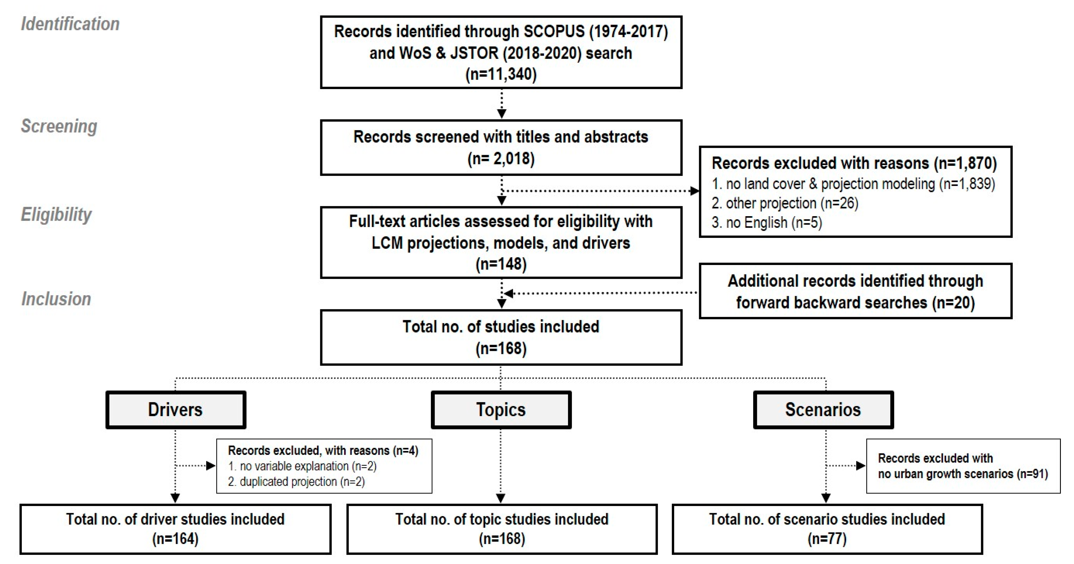
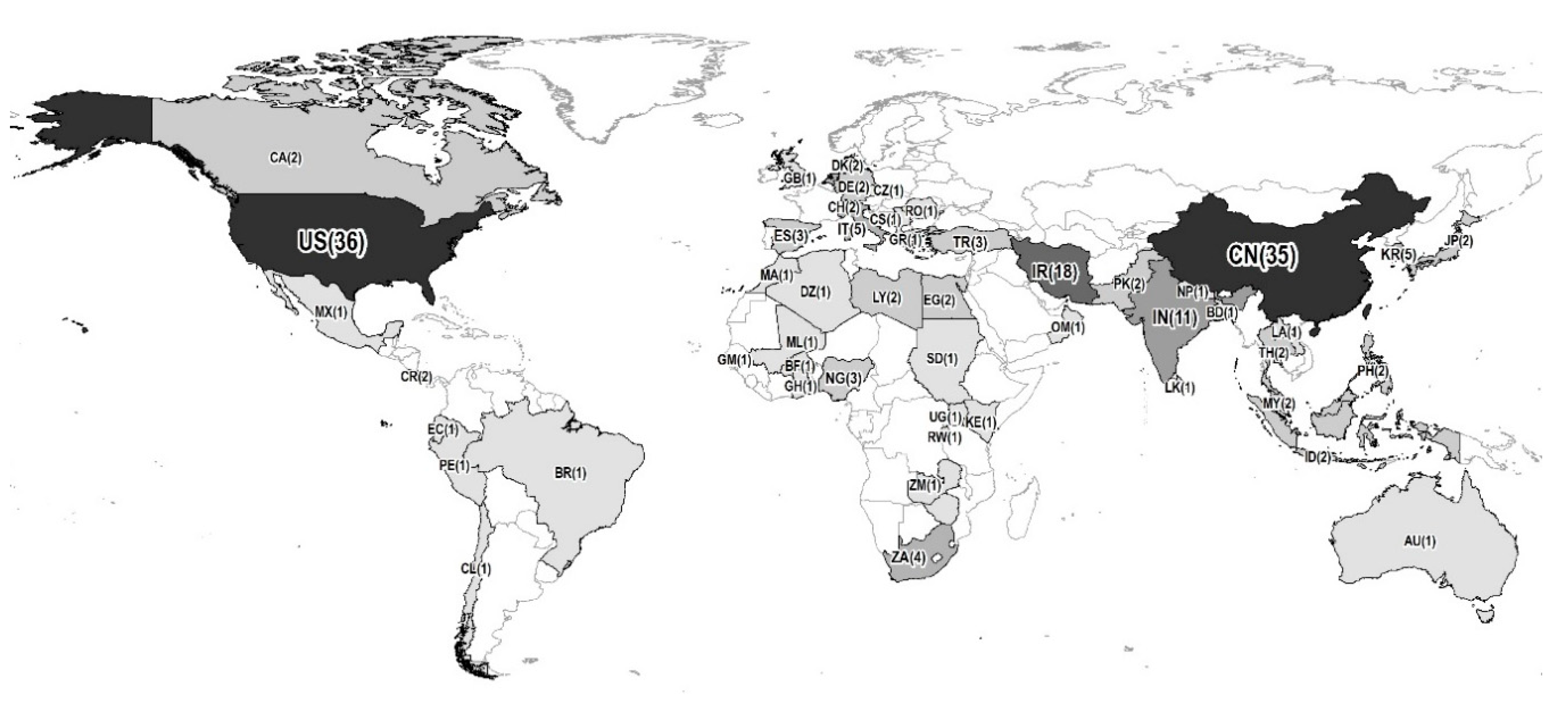
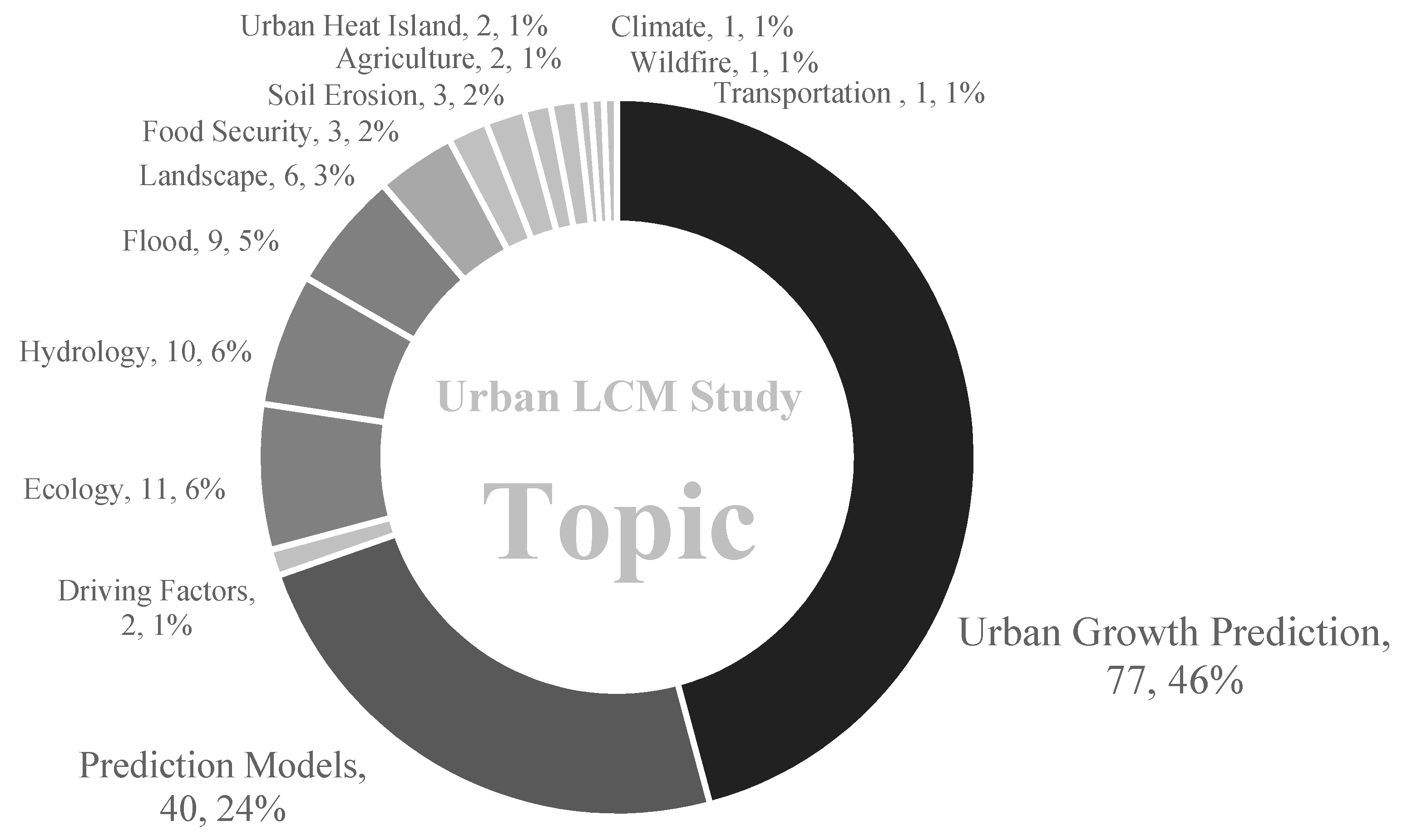
Table 1.
List of key driving factors in empirical studies.
| Classification | Driving Factors | Classification | Driving Factors | ||
|---|---|---|---|---|---|
| Natural Environment | Topography | slope | Built Environment | Land Use | distance to settlement |
| distance to river | land use | ||||
| distance to water surface | distance to city/district/town centers | ||||
| Amenity | distance to forest | distance to residence | |||
| distance to coastline | Job | distance to agriculture | |||
| distance to green spaces | distance to commercial | ||||
| distance to natural scenery | job location | ||||
| Built Environment | Transportation | distance to roads | Service | distance to schools | |
| distance to highways | distance to hospitals | ||||
| distance to railways | Socio-Economy | population density | |||
| distance to public transportation | property value | ||||
| Land Use | distance to settlement | land use plan | |||
| distance to urban center (CBD) | plan policies | ||||
Table 2.
List of predictor variables in the reviewed LCM articles *.
| Classification | ** Driving Factors | Count | Classification | Driving Factors | Count | ||
|---|---|---|---|---|---|---|---|
| Natural Environment (32) | Topography (14) | slope | 121 | Built Environment (53) | Land Use (13) | distance to town centers | 13 |
| elevation | 50 | likelihood to change | 11 | ||||
| distance to water surface | 37 | land use suitability | 3 | ||||
| distance to river | 35 | availability of irrigation facility | 1 | ||||
| aspect | 17 | density of crop land | 1 | ||||
| soil type | 11 | density of developed lands | 1 | ||||
| soil quality | 8 | Development (4) | distance to infra (water/sewer) | 8 | |||
| erosion | 6 | available land | 8 | ||||
| soil pH | 5 | cost of land use change | 2 | ||||
| soil permeability | 3 | recent development | 2 | ||||
| altitude | 2 | Job (12) | distance to agriculture | 21 | |||
| silt content | 2 | distance to commercial | 17 | ||||
| soil depth | 2 | distance to business | 8 | ||||
| terrain | 1 | distance to industrial | 7 | ||||
| Amenity (4) | distance to forest | 20 | distance to farm | 6 | |||
| distance to coastline | 14 | job location | 3 | ||||
| distance to green spaces | 6 | agricultural production | 2 | ||||
| distance to natural scenery | 4 | distance to economic corridors | 2 | ||||
| Climate (4) | precipitation | 10 | employment no. | 2 | |||
| temperature | 8 | industrial production | 2 | ||||
| hours of sunshine | 4 | density of oil and gas wells | 1 | ||||
| moisture | 1 | unemployment rate | 1 | ||||
| Risk (7) | flood risk (floodplain) | 7 | Service (3) | distance to institution | 14 | ||
| distance to wetland/salt marsh | 5 | distance to hospital | 3 | ||||
| seismicity | 3 | distance to convention | 1 | ||||
| distance to dike | 1 | Housing (3) | floor space entropy index | 2 | |||
| distance to tsunami affected area | 1 | housing density | 2 | ||||
| flood retention areas | 1 | floor space dissimilarity index | 1 | ||||
| water contamination | 1 | Socio-Economy (25) | Population (9) | population density | 42 | ||
| Ecology (3) | vegetation/env. value | 3 | population | 14 | |||
| tree type | 2 | race | 2 | ||||
| endangered species | 1 | household number | 1 | ||||
| Built Environment (53) | Transportation (18) | distance to major roads | 135 | housing growth rate | 1 | ||
| distance to highways | 24 | job density | 1 | ||||
| distance to railways | 20 | job housing balance | 1 | ||||
| distance to national/express highways | 13 | literacy | 1 | ||||
| distance to airport/harbor | 12 | urban population density | 1 | ||||
| distance to railway station | 11 | Plan (6) | distance to protected area | 13 | |||
| distance to minor roads | 8 | land use plan/policy | 8 | ||||
| distance to subway station | 7 | distance to city boundary | 4 | ||||
| distance to road junction | 6 | distance to historic sites | 3 | ||||
| distance to county roads | 5 | county boundary | 1 | ||||
| distance to motorway exits | 5 | state boundary | 1 | ||||
| distance to bus station | 4 | Economy (10) | GDP | 17 | |||
| distance to provincial roads | 4 | property/land value | 12 | ||||
| road density | 4 | income | 5 | ||||
| distance to metro station | 3 | employment rate | 3 | ||||
| distance to tollgate | 2 | poverty | 2 | ||||
| distance to bus route | 1 | rent | 2 | ||||
| transportation noise | 1 | industrialization rate | 1 | ||||
| Land Use (13) | distance to settlement | 74 | investment | 1 | |||
| distance to urban center (CBD) | 52 | investment on agri. research | 1 | ||||
| land use (land cover) | 49 | per capita foreign direct investment | 1 | ||||
| distance to residential | 35 | Others (3) | easting parameter | 5 | |||
| distance to (big) city | 25 | northing parameter | 5 | ||||
| distance to open land/recreation | 15 | crime | 1 | ||||
| distance to district centers | 13 | ||||||
| Total Driving Factor (113) | 1,215 | ||||||
* Drivers in SLEUTH model are counted as four (e.g., slope, land use, urban, and transportation) because hillshade and exclusion layers do not influence prediction results. Stochastic and duplicated neighborhood drivers are excluded in count. ** Drivers include factors affecting urban land uses (e.g., residential, commercial, industrial).
Table 3.
Scenario types in Land Change Modeling (LCM).
| Scenario Theme | Scenario Type | Reference | |
|---|---|---|---|
| Single | Ecology/Environment | business as usual, ecological/greenbelt | Romano et al. (2018) [121], Shi et al. (2017) [122], Park et al. (2017) [118], Goodarzi et al. (2017) [123], Lu et al. (2016) [109], Zheng et al. (2015) [61], Liu et al. (2015) [56], Akber and Shrestha (2015) [124], Zen et al. (2014) [125], Dezhkam et al. (2014) [126], Oguz (2013) [127], Xi et al. (2010) [117], Wu et al. (2010) [8], Wu and Martin (2002) [103] |
| Density | business as usual, sprawl, compact | Grigorescu et al. (2019) [128], Feng et al. (2019) [129], Shoemaker et al. (2019) [130], Henríquez-Dole et al. (2018) [131], Song et al. (2017) [132], Sakieh et al. (2015) [133], Terzi (2015) [98], Sekovski et al. (2015) [134], Bihamta et al. (2015) [135], Fuglsang et al. (2013) [120], Vermeiren et al. (2012) [136], Wilson and Weng (2011) [137], Benavente et al. (2010) [100], Tang et al. (2005) [138] | |
| Economic/Population Growth | business as usual, low and high economic/population growth | Bajracharya et al. (2020) [139], Huang et al. (2019) [27], Kuang (2011) [140], De Moel et al. (2011) [112], Allen and Lu (2003) [141], Bright (1992) [95] | |
| Plan | business as usual, planned/policy/managed/spatial planning | Zhao and Shen (2019) [142], Chakraborty et al. (2015) [143], Yuan (2010) [144], Hoymann (2010) [21], Hansen (2010) [145] | |
| Multiple | Growth and Environment | business as usual, economic growth, environmental/sustainable growth | Samie et al. (2017) [146], Hasan et al. (2017) [119], Liu et al. (2016) [51], Gallardo et al. (2016) [147], Han et al. (2015) [60], Plata-Rocha (2011) [148] |
| Density and Growth | business as usual, economic growth, sprawl/compact | Li et al. (2017) [26], Price et al. (2015) [149], Te Linde et al. (2011) [20] | |
| Density/Growth and Environment | business as usual, low and high growth, compact, environment | Kocabas and Dragicevic (2007) [54], Pettit and Pullar (2004) [96], Yang and Lo (2003) [114], Landis (1995) [113] | |
| Plan/Density and Environment | business as usual, planned, sprawl/compact, environmental scenario | Kim and Newman (2020) [150], Rimal et al. (2019) [151], Liang et al. (2018) [152], Lu et al. (2018) [153], Osman et al. (2016) [154], Kim and Park (2015) [155], Hua et al. (2014) [156], Liu et al. (2011) [157], Wu et al. (2010) [8], Gude et al. (2007) [158] | |
| Others | socio-economy, disaster, driver weight, different models, climate change, road weight, land cover change, development setback, weighting, agri. protection, growth location, global coordination | Li et al. (2020) [30], Chen et al. (2019) [29], Gibson et al. (2018) [159], Qiang and Lam (2016) [101], Gao and Kim (2016) [160], Shooshtari and Gholamalifard (2015) [64], He et al. (2015) [161], Chaudhuri and Clarke (2013) [116], Mahiny (2012) [162], Ray et al. (2010) [163], Kim (2009) [164], Lin et al. (2007) [111], Sharma et al. (2006) [49], Solecki and Oliveri (2004) [165], Hilferink and Rietveld (1999) [38] | |
© 2020 by the authors. Licensee MDPI, Basel, Switzerland. This article is an open access article distributed under the terms and conditions of the Creative Commons Attribution (CC BY) license (http://creativecommons.org/licenses/by/4.0/).
Share and Cite
MDPI and ACS Style
Kim, Y.; Newman, G.; Güneralp, B. A Review of Driving Factors, Scenarios, and Topics in Urban Land Change Models. Land 2020, 9, 246. https://doi.org/10.3390/land9080246
AMA Style
Kim Y, Newman G, Güneralp B. A Review of Driving Factors, Scenarios, and Topics in Urban Land Change Models. Land. 2020; 9(8):246. https://doi.org/10.3390/land9080246
Chicago/Turabian StyleKim, Youjung, Galen Newman, and Burak Güneralp. 2020. "A Review of Driving Factors, Scenarios, and Topics in Urban Land Change Models" Land 9, no. 8: 246. https://doi.org/10.3390/land9080246
Note that from the first issue of 2016, this journal uses article numbers instead of page numbers. See further details here.