Article

Land Consumption Dynamics and Urban–Rural Continuum Mapping in Italy for SDG 11.3.1 Indicator Assessment

by
Angela Cimini
1,
Paolo De Fioravante
2,*,
Nicola Riitano
3,
Pasquale Dichicco
2,
Annagrazia Calò
2,
Giuseppe Scarascia Mugnozza
4,
Marco Marchetti
5 and
Michele Munafò
2
1
Department of Architecture and Project, University of Rome La Sapienza, Piazza Borghese 9, 00186 Roma, Italy
2
Italian Institute for Environmental Protection and Research (ISPRA), Department of Networks and Environmental Information Systems (SINA), Via Vitaliano Brancati 48, 00144 Rome, Italy
3
Italian Institute for Environmental Protection and Research (ISPRA), Department for the Geological Survey of Italy, Via Vitaliano Brancati 48, 00144 Rome, Italy
4
Department for innovation in Biological, Agro-Food and Forest Systems, University of Tuscia, Via S. Camillo de Lellis, 01100 Viterbo, Italy
5
Dipartimento di Bioscienze e Territorio, Università degli Studi del Molise, C/da Fonte Lappone, 86090 Pesche, Italy
*
Author to whom correspondence should be addressed.
Land 2023, 12(1), 155; https://doi.org/10.3390/land12010155
Submission received: 24 November 2022 / Revised: 21 December 2022 / Accepted: 28 December 2022 / Published: 3 January 2023
(This article belongs to the Special Issue Dynamics of Urbanization and Ecosystem Services Provision)

Abstract

:
For the first time in human history, over half of the world’s population lives in urban areas. This rapid growth makes cities more vulnerable, increasing the need to monitor urban dynamics and its sustainability. The aim of this work is to examine the spatial extent of urban areas, to identify the urban–rural continuum, to understand urbanization processes, and to monitor Sustainable Development Goal 11. In this paper, we apply the methodology developed by the European Commission-Joint Research Center for the classification of the degree of urbanization of the Italian territory, using the ISPRA land consumption map and the ISTAT population data. The analysis shows that the availability of detailed and updated spatialized population data is essential to calculate SDG indicator 11.3.1, which assesses the ratio of land consumption rate to population growth rate. Three new indicators are also proposed to describe the main trends in urban sprawl, analyzing the spatial distribution of land consumption in terms of infill and settlement dispersion. The research shows good results in identifying class boundaries and describing the Italian urbanized landscape, highlighting the need for more detailed spatialized demographic data. The classification obtained lends itself to a variety of applications, such as monitoring land consumption, settlement dynamics, or the urban heat islands, and assessing the presence and state of green infrastructures in the urban context, driving the development of policies in urban areas toward sustainable choices focused on urban regeneration.

1. Introduction

1.1. Effects of Urban Growth and Insights on Urbanization Dynamics in Italy

Historically, the main drivers of urban development have been economic and demographic growth but also the effects of local policies and regulations [1,2]. In recent years, the extension of city surface areas has been increasing twice as fast as their population, leading to an estimated increase in global land consumption of 1.2 million square kilometers by 2030 [3]. This expansion will have repercussions on the habitats and ecosystem, influencing the services they provide to humans and other life on Earth [4], e.g., they can lead to hydrological impacts, influencing runoff in urban catchments [5] and crop production [6]; moreover, urban centers are responsible for about 70% of global carbon emissions and more than 60% of resource use, while rapid urbanization is often associated with worsening air pollution [7,8,9]. These considerations were strengthened after the emergency linked to the COVID-19 pandemic, which highlighted the need for resilient cities that guarantee the highest level of well-being to citizens [10,11]. Human pressure on soil is a key driver of the loss of biodiversity and of ecosystem services [12]. Due to their high density of people and assets, cities must play a central role, which is manifested in one of the sustainable development goals formulated by the United Nations within the 2030 Agenda. The 17 Sustainable Development Goals and the 169 associated targets integrate and balance the three dimensions of sustainable development, covering social, economic, and environmental aspects [13]. The thematic of the SDG 11 is the “Sustainable Cities and Communities” [14]; to monitor progress toward the achievement of target 11.3 (“by 2030 enhance inclusive and sustainable urbanization and capacities for participatory, integrated and sustainable human settlement planning and management in all countries”), the UN established indicator 11.3.1, which measures how efficiently cities use the territory, focusing on the relation between urban expansion and the population growth in urban area [15]. This indicator is categorized under Tier II, meaning the indicator is conceptually clear and an established methodology exists but data on many countries are not yet available [16,17,18].
In this context, it is essential to understand the state of settlements and the main trends in urbanization and demographic variations. The low-density urban growth known as “sprawl” [19,20] is a common phenomenon in Europe that, in Italy, assumes the characteristics of extreme dispersion, taking the name of “sprinkling” [21]. Compared to sprawl (which is based on urban systems designed through zooning), this settlement dynamic develops spontaneously, following different intensities based on the orography and often in the absence of urban planning. Sprinkling is characterized by aggregates of highly variable dimensions that generate low-density hybrid landscapes in rural areas, whose characteristics mix with those of urban areas [22,23,24] (Figure 1). This configuration is the result of planning processes of the 1960s and 1970s, which led, on the one hand, to the creation of new zone plans on the peripheral areas and to densification, and on the other, to the construction of new residential complexes in the countryside. This dynamic has led to the proliferation of settlements in a widespread form on the margins of large urban centers, influencing the growth of periurban fringes and the transposition of urban models to the countryside [25]. Therefore, on the one hand, there is the presence of consolidated urban forms with centrality roles, and on the other, discontinuous and low-density suburban or periurban settlements have been formed, with marginal dimensions and roles that limit the triggering of centrality effects [26]. This fraying of the margins of urban areas makes the delimitation of the margins between city and countryside complex and limits the definition of a univocal criterion for circumscribing them [27]. It is, therefore, necessary to analyze the urban landscape on a national scale in terms of the urban–rural continuum, overcoming the urban–rural dichotomy [28,29,30].

1.2. Existing Data for the Representation of Urban Areas

Several products are available nationally and internationally for the representation of urban areas and the urban–rural continuum, with different geometric and thematic characteristics and different definitions.

1.2.1. Global Data—Global Human Settlement Layer (GHSL) SMOD

Eurostat proposes a harmonized methodology to improve the quality of urban statistics starting from the classification of the entire territory along an urban–rural continuum. The scheme is based on the combination of population data (represented by a grid of 1 km²) and density of artificial surfaces, with the aim of overcoming the traditional urban–rural dichotomy [28,30]. The Joint Research Center (JRC) has implemented Eurostat’s methodology by introducing the Global Human Settlement Layer (GHSL), which offers information on a global scale, based on the combination of total resident population density [31,32].

1.2.2. European Data—Copernicus Land Monitoring Service Data

Copernicus data refer to a definition of urban area that considers permanently populated areas and surfaces dominated by the influence of human activities, excluding agricultural use. These areas include all man-made structures (buildings, road infrastructures, and other paved areas) and the unsealed and vegetated surfaces associated with them.
The CORINE Land Cover (CLC) belongs to the Pan-European component of the CLMS and describes land cover and land use with a minimum mapping unit of 25 hectares for the entire European territory. Class 1 CLC distinguishes “artificial areas” according to the prevalent use into “Urban fabric” (which includes built-up areas), “Areas mainly for commercial and industrial use and infrastructures for transport and logistics” (such as ports, airports, roads, and railways), “Quarries, landfills and construction sites”, and “Green urban areas and sport and leisure facilities” [33,34,35].
Urban Atlas (UA) is another important CLMS data for the description of urban areas. UA belongs to the Local component of the CLMS and provides a high-spatial-resolution land cover and land use mapping of Functional Urban Areas (FUAs), defined as the set of central cities and their commuting areas. The data are available for the years 2006, 2012, and 2018 and have a higher spatial resolution for artificial classes (minimum mappable unit of 0.25 hectares) than for natural areas (1 hectare). There are also two change layers, relating to the periods of 2006–2012 and 2012–2018. Urban Atlas adopts a four-level classification system based on CLC classes, with higher thematic detail for artificial areas [36].

1.2.3. European Data—European Settlement Map

The European Settlement Map (ESM) is a mapping of the human settlements in Europe produced with GHSL technology by the Joint Research Center (JRC) and represents the percentage of built-up area coverage per spatial unit. The ESM for 2016 was obtained by applying machine learning techniques on multispectral and panchromatic bands of SPOT5 and SPOT6 imagery, in order to understand systematic relations between morphological and textural features in the description of human settlement [37,38].

1.2.4. National Data—Degree of Artificialization and Degree of Urbanization

ISPRA has characterized the urban–rural continuum according to two approaches, based on the analysis of the density of artificial surfaces (in the first case) and integrating this information with data on population density (in the second one).
The first approach describes the density of the artificial surfaces starting from the ISPRA National Land Consumption Map (LCM), considering the average density of the artificial surfaces in a radius of 300 m. The LCM is a 10-m-resolution raster, produced and updated annually [39,40,41]. The data have national coverage and are available for the years 2006, 2012, and all the years between 2015 and 2021. The map adopts a three-level classification system, which distinguishes different classes of permanent and reversible consumed land [42]. The third classification level is adopted for all new changes and is available for most of the built-up areas, for the entire road network, and for all quarries, landfills, and paved and unpaved greenhouses. The national territory was then classified into urban, suburban/periurban, and rural areas, in accordance with the thresholds indicated by sustainable development goal number 11 of the United Nations 2030 Agenda.
The second ISPRA data is based on a procedure similar to the Eurostat/JRC one and considers the consumed land density map together with the population density map. The resulting data have four classes of artificial surface and population density, three of which reflect those of the Eurostat/JRC (High-Density Urban Areas, Medium-Density Urban Areas, and Rural Areas) and the fourth relates to areas with a high density of artificial surfaces and low population density [42].

1.3. Describe Urban–Rural Continuum Using National Data

The study proposes a classification of urban areas for the Italian territory according to the indications of the 2030 Agenda for Sustainable Development and the related Sustainable Development Goals. The research is part of the activities carried out by ISPRA for the characterization of the rural-urban continuum and for the monitoring and analysis of the spatial distribution of land consumption [42]. For this purpose, the methodology adopted by Eurostat and applied by JRC for the realization of the GHS-SMOD was resumed and adapted to the ISPRA LCM and to the ISTAT demographic data. Starting from this characterization of the urban area, an estimate of the SDG 11.3.1 indicator and of the land consumption distribution was carried out for the period 2012–2018.

2. Materials and Methods

2.1. Overview

The study refers to the entire Italian territory (Figure 2) and takes up the methodology proposed by Eurostat for a classification of the urban–rural continuum based on the spatial distribution of the population.
Three main phases can be identified:
  • Creation of a spatialized population layer based on ISTAT demographic data.
The spatial distribution of the population was analyzed starting from the ISTAT data on total municipal population, considering for each municipality a uniform distribution of the inhabitants among the “residential” pixels. Ancillary data were introduced to identify the residential areas: Starting from the LCM, the buildings were identified and then, using the CLMS and ESM data, the residential ones were selected.
2.
Classification of the urban–rural continuum on a national scale starting from the spatialized population data.
Through focal analysis, the population density was evaluated around 1 km2 of each pixel and population density thresholds were introduced to identify 4 classes of clusters, which were then further divided into 9 subclasses based on the total population and contiguity rules.
3.
Application of the classification of the urban–rural continuum for the calculation of SDG indicator 11.3.1.
The metadata of the SDG 11.3.1 indicator suggest calculating the “Ratio of land consumption rate to population growth rate” considering the urban area obtained by applying the Eurostat/JRC methodology as the reference area. However, the most detailed and updated demographic data for Italy refers to the aggregate value of total municipal population. Actually, no further information is available on the spatial distribution of the population and its variations among the different urban–rural classes within the same municipality (for example, how many inhabitants of a municipality live in its urban center or the migrations from urban to periurban/suburban or rural and vice versa). As suggested by Eurostat, each municipality was associated with the prevailing class (the one in which the largest number of inhabitants lived) and the calculation of the indicator was carried out for the entire territory of the urban municipalities, i.e., those where the urban class prevails. To provide information on the evolution of urbanized areas within the municipal territory, three new indicators were introduced that evaluate the distribution of land consumption among the urban suburban/periurban and rural classes.

2.2. Spatialization of the Population

This paragraph describes the procedure for creating a spatialized population layer based on ISTAT demographic data (Figure 3). The analysis refers to 2018 and is conducted for the entire national territory.
ISTAT provides yearly updated population data for the Italian territory, with the highest level of detail at the municipal scale (total municipal population). According to the Eurostat methodology, in the absence of spatialized population data (geocoded census or population register), a disaggregation grid can be created by combining the population of census units with high-resolution land use data from national or global sources [31]. To allocate the population within the territory of the municipalities, ancillary data were introduced for the identification of residential areas. First, the built-up areas were identified, starting from the ISPRA LCM, where areas classified as 111 (buildings) and as 1 (consumed land not yet reclassified to the third thematic level of detail) were selected. Starting from these built-up areas, residential buildings were identified using the Copernicus CLMS data (CORINE Land Cover, Urban Atlas, Coastal Zones, Natura 2000 and Riparian Zones) and the ESM data. CLMS class 1 distinguishes different artificial surfaces, making it possible to separate the “urban fabric” from “industrial, commercial, transport, and logistics areas”, “extraction sites”, “green urban areas”, and “sport and leisure facilities”. In areas not covered by CLMS class 1, ESM was used, which provides thematic information on residential and non-residential buildings derived by remote sensing imagery and training data. For each municipality, the total population of ISTAT was spatialized considering a uniform distribution among the “residential building” pixels, as no supporting data are available (such as the height of the buildings or updated census sections) to distribute the population on the municipality in a more detailed way. In the following, we refer to the spatialized population data as “population raster”.

2.3. Classification of the Urban–Rural Continuum

This paragraph describes the methodology for the classification of the urban–rural continuum on a national scale starting from the population raster. The analysis refers to 2018 and is conducted for the entire national territory.
The classification adopted by Eurostat and JRC requires information on population density per square kilometer. These data were obtained by calculating the focal statistics on the population raster and associating with each pixel its own population density value around 1 km2. The data were, therefore, reclassified into four classes, according to the following thresholds (Table 1):
  • Class 1, with over 2000 inhabitants per km2;
  • Class 2, for areas with between 500 and 2000 inhabitants per km2;
  • Class 3, for areas with between 100 and 500 inhabitants per km2;
  • Class 4, with less than 100 inhabitants per km2.
Class 1 was further subdivided based on the total population, making it possible to identify:
  • Urban Centers with over 2000 inhabitants per km2 and a population of over 10,000 inhabitants;
  • Dense Urban Clusters with over 2000 inhabitants per km2 and a population of less than 10,000 inhabitants.
Class 2 was divided into two subclasses using a contiguousness criterion:
  • Suburban cells, for areas contiguous to class 1 and with a population density between 500 and 2000 inhabitants per km2;
  • Semi-dense Urban Clusters, for areas not contiguous to class 1 and with a population density between 500 and 2000 inhabitants per km2 and a total population of over 5000 inhabitants;
  • Rural Clusters with population density between 500 and 2000 inhabitants per km2 and a population of less than 5000 inhabitants.
Class 4 was defined “Low-Density Rural Cells”, while the areas that do not fall into any of the above classes were classified as “Very Low-Density Urban Cells”. An additional class was also introduced with respect to the Eurostat and JRC classification, relating to areas with high built-up density and low population density, which are mostly associated with production, commercial, or logistics areas. This class was identified with a focal analysis on non-residential buildings and includes areas that have a built density higher than 10% in an area of 1 km2.
The Eurostat/JRC thresholds were revised through trial and error in order to take into account the characteristics of the population raster, maintaining a result as comparable as possible to the GHS-SMOD. In detail, the population raster compared to the GHS-SMOD has a higher spatial resolution (10 m against 1 km) and, for the spatialization of the population, it does not consider the census sections, whose data are updated to 2011.

2.4. Calculation of the SDG 11.3.1 Indicator

The paragraph describes the application of the classification of the urban–rural continuum for the calculation of SDG indicator 11.3.1. The calculation was conducted with respect to the period of 2012–2018 on urban municipalities, i.e., those in which the population is mainly concentrated in the urban classes. Here, a set of three unpublished indicators was also calculated to analyze the spatial distribution of land consumption among the urban, suburban/periurban, and rural classes.

2.4.1. SDG 11.3.1 Indicator

The indicator SDG 11.3.1 “Ratio of land consumption rate to population growth rate” (RLCRPGR) relates the variation in land consumption with the variation in population in a reference period. In detail, it is defined as the ratio of land consumption rate (LCR) to population growth rate (PGR) [16]:
RLCRPGR = LCR PGR   = [ ( C L t + n C L t C L t ) T ] [ l n   ( P o p t + n P o p t )   y ]
where:
C L t = Total areal extent of the consumed land for the first year.
C L t + n = Total areal extent of the consumed land for the last year.
T = Number of years between CLt+n and CLt.
P o p t = Total population in the first year.
P o p t + n = Total population in the last year.
y = Number of years between the two measurement periods.
The indicator metadata suggest calculating the RLCRPGR assuming the territory classified as an urban area as the reference area, according to the Eurostat/JRC methodology. The assessment requires deep knowledge of the spatial distribution of land consumption and population variation, in order to be able to accurately evaluate the variation in the two quantities within the reference urban area.
With regard to the LCR, the LCM provides spatialized and yearly updated information on land consumption, allowing for the identification of the changes occurring in the reference urban area.
Regarding the PGR, ISTAT produces and annually updates the official demographic data for Italy, providing the total municipal population as more detailed data. These data do not allow for spatially characterizing in which areas of the municipality population variations occur. Actually, it is not possible to evaluate the population variation with respect to urban areas, as, in some cases, they only occupy a portion of the municipal territory, and in others, they include more municipalities. In accordance with the Eurostat/JRC methodology, the calculation was, therefore, carried out on a municipal scale, associating the prevailing urban–rural class with each administrative unit (i.e., the one in which the majority of the population is concentrated) [31]. The indicator was calculated for the period 2012–2018 on the municipalities classified as “Urban Center”, “Dense Urban Cluster”, and “Semi-dense Urban Cluster”.
The value of the indicator depends on the two terms LCR and PGR. If they are both positive (increase in land consumption and population) or negative (decrease in land consumption and population), the indicator assumes positive values; otherwise, it is negative. For the interpretation of the RLCRPGR indicator, it is important to observe the sign of LCR and PGR, as the same RLCRPGR value can represent different dynamics (for example, a negative RLCRPGR value can derive from an increase in PGR and a decrease in LCR or from an increase in LCR and a decrease in PGR) (Table 2).

2.4.2. Normalized Difference of Consumed Land

In addition to the calculation of SDG 11.3.1, the auxiliary indicator “Normalized Difference of Consumed Land” (NDCL) was also introduced, with reference to urban areas (2), suburban/periurban areas (3), and rural areas (4):
NDCL u = LC   in   urban   area     LC   in   rural   and   suburban   area Total   LC  
NDCL s = LC   in   suburban   area     LC   in   rural   and   urban   area Total   LC
NDCL r = LC   in   rural   area   LC   in   urban   and   suburban   area Total   LC  
The indicators were calculated for the same urban municipalities considered for the RLCRPGR indicator. The calculation was based on the ISPRA LCM for the two reference years and the interpretation of the three indicators allows for describing the spatial distribution of land consumption in the urban municipalities. Each of the three indicators evaluates the portion of land consumption that affects each of the three classes (urban, suburban/periurban, and rural) and the one that assumes the highest value represents the prevailing trend of that municipality, in terms of:
  • Urban Infill, where land consumption mainly affects urban areas, thus filling the gaps between the existing urban fabric.
  • Periurban Infill, when land consumption is concentrated in periurban areas on the edge of the dense urban fabric.
  • Dispersion, when low-density land consumption occurs in rural areas.

3. Results

3.1. Spatialization of the Population

The spatialization of the population refers to the residential areas identified on the ISPRA LCM. Starting from the total consumed land of the LCM (2,130,088 hectares in 2018), buildings (class 111) and consumed land at the first classification level (class 1) were selected, for a total of 536,579 and 689,645 hectares, respectively. The introduction of CLMS and ESM data made it possible to distinguish the residential component (71.42% of the built-up area) from the non-residential component (28.57% of the built-up area) (Table 3), where the population was evenly distributed.

3.2. Classification of the Urban–Rural Continuum

The classification of the settlements of the national territory according to the eight Eurostat/JRC classes provided the results shown in Figure 4 and Figure 5 and Table 4, expressed in terms of hectares and percentages on the national surface. The data were also compared with the GHS-SMOD data.
The Italian territory shows a prevalence of rural classes with low and very low population density. The areas with the highest population density (Urban Centers and Dense Urban Clusters) occupy just over 2% of the national territory, while the surrounding suburban areas occupy under 5%. Compared to the GHS-SMOD, there is a similar distribution of the national territory between urban, suburban/periurban, and rural classes, with the main differences concerning the classes of Dense Urban Cluster and Semi-Dense Urban Cluster, which are larger in the GHS-SMOD than in the proposed data.
A total of 2825 urban clusters are identified on the national territory, of which 719 are classified as Urban centers, 2046 as Dense Urban Clusters, and the remaining 60 as Semi-Dense Urban Clusters (Table 5). Overall, the Urban Centers occupy about three times the surface of the Dense Urban Clusters and over 10 times that of the Semi-Dense Urban Clusters. About half of the Urban Centers are in Lombardy (which accounts for a quarter of the class), Campania, and Lazio. Lombardy is also the region where the class of Dense Urban Clusters is most extended, while about one third of the Semi-Dense Urban Clusters fall in Veneto, Latium, and Sicily.
Regarding the extension of the larger urban centers, in Lombardy and Campania, the centers of Milan and Naples each occupy almost 50,000 hectares, while, in Latium, the urban area of Rome reaches just under 40,000 hectares. In the other regions, the main centers do not reach 10,000 hectares, except for Piedmont and Sicily, which stop just above this threshold. The “Largest Urban Patch Index” (LUPI) expresses the extent of the largest patch as a percentage on the total regional extent of the three urban classes. In Campania and Latium, the two main clusters are among the largest in Italy and occupy between 50 and 60% of the regional urban class, while Lombardy’s Milan cluster, despite being the largest in Italy, includes less than a third of regional urban areas, reflecting the high level of urbanization of this region. The highest LUPI value is in the Valle d’Aosta, where the Aosta cluster (despite being the smallest of the largest regional urban centers) includes over 70% of the urbanized area of the region, confirming the low level of artificialization of that territory.

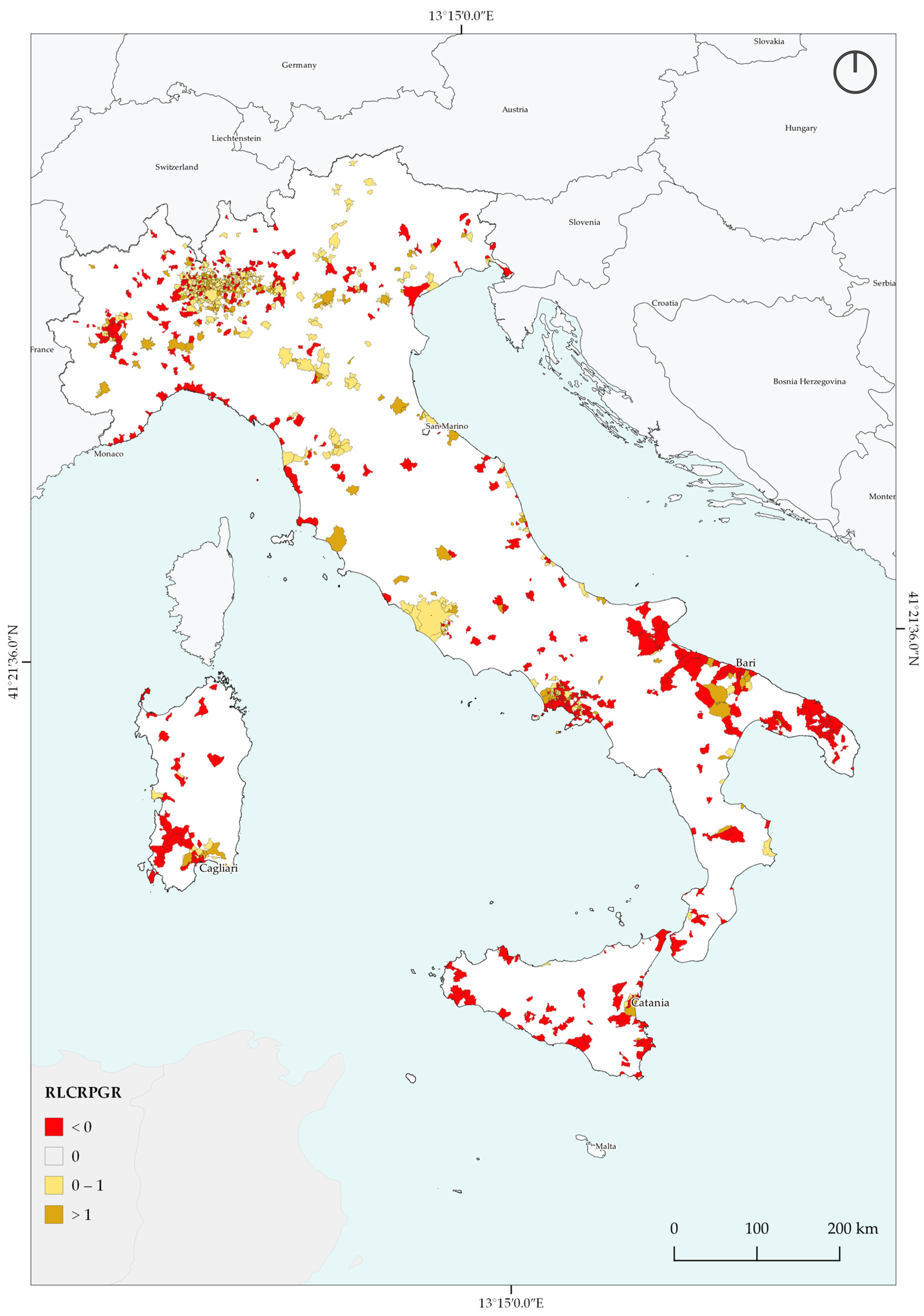
3.3. Calculation of the SDG 11.3.1 Indicator

The attribution of the prevailing urban–rural class to the municipalities provided the results of Table 6 and Figure 6 and Figure 7.
For the calculation of the RLCRPGR indicator, municipalities defined as “Urban Center”, “Dense Urban Cluster”, and “Semi-dense Urban Cluster” were taken into consideration (Figure 7). Overall, 1131 municipalities belong to the three classes (14% of the total), of which 605 classified as Urban Center, 470 as Dense Urban Cluster, and 56 as Semi-dense Urban Cluster.
The calculation of the RLCRPGR indicator provided the values shown in Figure 8, relating to municipalities with an increase in land consumption and, therefore, positive LCR values. In detail, 13 of the 1131 municipalities show negative LCR values; in 6, there are no changes in LCR, and 1112 show an increase in land consumption. For all urban municipalities with a decrease in land consumption (LCR < 0), the whole territory was inspected using the ISPRA LCM. In all cases, the restorations take place in areas classified as reversible land consumption, in correspondence with areas of maneuvering and storage surrounding the construction sites of new buildings, roads, and infrastructures, as in the example of Figure 9. The following analysis, therefore, focused only on municipalities with LCR > 0.
With regard to the municipalities with increasing land consumption, the following results were obtained (Figure 10):
  • In 571 municipalities (51.3% of those with LCR > 0), the indicator has values less than 0. In these areas, the increase in land consumption corresponds to a decrease in population. In detail, in the 397 municipalities with SDG values between 0 and −1, the rate of population decrease is significantly higher than the rate of increase in land consumption, while in the 174 municipalities with SDG < −1, the increase in land consumption is higher than the population decrease.
  • The SDG has positive values in 541 municipalities (48.6% of urban municipalities with increasing land consumption). About two thirds of them have values between 0 and 1, i.e., a rate of increase in the population higher than the rate of increase in land consumption, while in the remaining 164 municipalities, the population increases less than the increase in land consumption.
The SDG indicator was supported by an analysis on the territorial distribution of land consumption between urban, periurban/suburban, and rural areas relating to the period of 2012–2018 (Table 7).
Land consumption between 2012 and 2018 prevails in rural areas; in fact, over one third of the changes fall into the “Rural Cluster”, “Rural Low Density”, and “Rural Very Low Density” classes. Urban classes and periurban/suburban areas each host about a quarter of the total changes, while about 17% of land consumption is in non-residential areas for productive and commercial use. The trend toward land consumption outside the denser urban classes is also recognizable from the analysis of the three Normalized Difference of Consumed Land (NDCL) indicators, which describe the prevailing trend in each of the analyzed municipalities. The three indicators NDCLu, NDCLs, and NDCLr assume values between −1 and 1 and, for each municipality, they have a sum equal to -1; the one with the highest value indicates the prevailing tendency of land consumption to be concentrated in urban areas (prevalence of NDCLu), periurban/suburban areas (prevalence of NDCLs), or rural areas (prevalence of NDCLr).
The calculation of the three indicators for the 1131 urban municipalities shows the results of Figure 11 and Figure 12, with a tendency to infill in the main provincial municipalities and a concentration of land consumption in the rural area in the other municipalities, with a tendency toward dispersion in areas with low settlement density.
In detail (Table 8), in 493 municipalities, land consumption is concentrated in rural areas (settlement dispersion). In 317 municipalities, land consumption has the characteristics of the completion of periurban/suburban areas, and in the remaining 321 municipalities, it shows a tendency to infill the voids between the dense and semi-dense consolidated urban fabric.

4. Discussion

The availability of adequate input data for the description of the spatial distribution of built-up areas and population is one of the main factors influencing the representation of settlements in compliance with the Eurostat methodology [17,43]. ISPRA LCM represents the built-up areas on the Italian territory with high thematic and spatial detail and yearly updates [40,42], while, at the European level, the CLMS data allow a description of the artificial areas LU with good coverage and high thematic detail while maintaining an adequate update frequency (indicator SDG 11.3.1 recommends conducting the calculation over a reference period of 5–10 years) [16]. Finally, on a global scale, it is possible to study urban areas starting from the classification of artificial surfaces obtained from free satellite data, such as Sentinel-2 multispectral images or Sentinel-1 SAR data [41]. Currently, the main limitation is linked to the availability and homogeneity of demographic data [44]. ISTAT data are the national reference for demographic analysis in Italy and they are updated yearly for the national scale and at NUTS 2, NUTS 3, and municipal levels [45]. In this study, the availability of high-resolution LU data has made it possible to uniformly spatialize the population on the residential areas of each municipality; however, the absence of an updated spatialized population data limits the possibility of carrying out analysis on a local scale, for example, linked to population flows between different urban clusters of the same municipality. A version of the data with higher spatial detail refers to the census sections but is subject to ten-year updates, since 1991, 2001, and 2011 [46], and the data as of 2021 have not yet been published.
The proposed representation of the urban–rural continuum is in line with Eurostat indications, adapting to the specificities of the Italian territory and bringing the description of these areas to a higher level than the ISPRA “degree of urbanization” [42]. The data show a concentration of urban areas along the coastline, in lowland areas, and in the valley floors, particularly in the Po valley. At the regional level, Lombardy has the largest extension and the highest number of urban clusters (about 18% of large urban centers, dense urban clusters, and semi-dense urban clusters are in this region). The yellow (suburban/periurban areas) and light green (rural low-density areas) areas show that the expansion of the urban clusters is concentrated along the main road infrastructures (Figure 5, Table 4, and Table 5). Compared to the GHS-SMOD, the data allow for yearly updates and the use of LCM offers a better description of the low-density built-up areas typical of the sprinkling of Italian rural and periurban landscapes. Moreover, the introduction of the class of “Industrial, commercial, and services” areas, which occupy 1.47% of the total national surface, makes it possible to understand their position and role with respect to the urban–rural continuum, which constitutes a useful support tool for orienting effective governance policies for the sustainable management of productive areas [47].
The classification of the urban–rural continuum was used to calculate the SDG 11.3.1 indicator on Italian urban areas. The LCM adequately identifies land consumption within urban areas, while the population data do not allow for intra-municipal analysis. The calculation of the RLCRPGR was, therefore, carried out on a municipal scale, associating with each municipality the class of the urban–rural continuum where most of the population is concentrated; the RLCRPGR was then calculated in municipalities classified as “Urban Center”, “Dense Urban Cluster”, and “Semi-dense Urban Cluster”. The calculation of RLCRPGR conducted on urban municipalities highlighted an increase in land consumption in 1112 of the 1131 urban municipalities considered (over 98% of the total), and half of them show a decrease in the population (571 of the 1131 considered municipalities), indicating a disconnection between land consumption and population variation; however, the lack of spatialized population data prevents an exact assessment of the migration flows within the administrative boundaries of the municipality, limiting the effectiveness of the RLCRPGR indicator. To better understand the dynamics occurring within the territory of the urban municipalities, a set of new indicators was also introduced for the assessment of the spatial distribution of the land consumption that occurred between 2012 and 2018, evaluated on the ISPRA LCM. The analysis of the distribution of changes between the different classes of the urban–rural continuum shows a tendency to fill urban voids in the consolidated built-up area (infill), which affects 28.38% of the 1131 urban municipalities considered. A similar percentage (28.03%) of the municipalities shows a tendency toward the expansion of the cities in the periurban fringes (periurban infill), while, in the remaining 43.59% of the urban municipalities, the land consumption is concentrated in the low-density rural areas, confirming the consolidated trend toward sprinkling. This trend affects the rural areas located on the edge of the dense urban core, which are subject to a conversion and a fusion in periurban fringes.
The application of the Eurostat/JRC methodology to the Italian context shows encouraging results, improving the representation of the territory compared to other current available national and international data. The distinction between low-density clusters and surrounding periurban areas can be further improved, but more detailed information on the spatial distribution of the population would be needed. Furthermore, the future introduction of LU information on the LCM will also allow a more accurate discrimination of residential areas from non-residential ones; the integration with an auxiliary database (i.e., satellite images and socioeconomic data) could support the creation of dasymetric maps useful for improvement of the limitation related to the availability of disaggregated census data [48].

5. Conclusions

Historically, city size and economic growth have been described as strictly correlated [49] and, in combination with population growth, have generally driven land consumption dynamics. This paradigm has lost its validity in recent years; indeed, the significant urban growth detected in recent decades is completely unrelated to the demographic dynamics both in Italy and at a global scale [3]. Furthermore, the intense migratory flow to urban areas has led to an unplanned growth of cities, which usually expand their geographic boundaries [50]. In this context, monitoring the state and evolution of urban areas is essential for defining strategies aimed at sustainable management and development of settlements [51].
Regarding spatial expansion, the historical evolution of the Italian landscape has led to an increase in land consumption in rural areas, and, in particular, in the urban fringe, assuming the characteristics of sprinkling and causing a low-density expansion of the urban fabric toward the surrounding areas [52]. This trend has led to a shift from a landscape in which a dichotomy between urban and rural areas was clearly distinguishable, to a continuum where dense urban fabric expands and merges with the surrounding rural areas, generating large and dilated suburban and periurban bands [29]. In this context, it is necessary to define and orient the planning tools in such a way that they capture these specificities of the territory and adequately orient the decision-making processes, while remaining connected with the European framework in terms of achieving the sustainable development goals.
This study falls within the framework of the research activities carried out by ISPRA for the definition of tools for the monitoring of land consumption and its influence on urban areas and for the characterization of settlement dynamics [39,40,41,42,53,54,55]. These topics are also of interest at the legislative level; the proposed law on urban regeneration [56] and the future national law on land consumption (envisaged among the reforms of the PNRR) [57] underline the need of tools for monitoring land consumption and the effectiveness of urban regeneration interventions, functional to the conservation of natural and semi-natural areas within and outside the urban area. The monitoring activity should be ensured at different scales of investigation and be based on scientific data collected in representative contexts of the urban area, in order to provide data and information to support decision-making and land-government activities.
The presented work fits within this request by providing a geographic interpretation of the urban–rural continuum of the whole national territory with high geometric detail, allowing for the analysis of settlement dynamics within urban areas and in the surrounding landscape, to make comparisons between different contexts and to stand as a supporting basis for further multi-scalar analysis [58,59]. Along these lines, future insights will involve analysis of urban morphology even at the neighborhood scale with the aim of identifying recurring and recognizable settlement types that can support strategies to restore the urbanized landscape in accordance with the physical elements that compose it [60,61,62,63,64,65]. Actually, this representation of the urban–rural continuum has the characteristics to be a reference for a wider range of further analysis at the regional scale, such as the management and conservation of urban green infrastructures [66,67] or the monitoring of the Urban Heat Island along the urban–rural continuum [68,69], and can support activities related to the introduction of nature-based solutions [67] or with the study of the fragmentation of urban forms [70].
This study shows that the availability of appropriate input data significantly affects the quality of the resulting monitoring tools. The input data introduced for the description of land consumption and the population have yearly updates, allowing the data to be updated with a high frequency. In addition, the introduction of high-spatial-resolution data for the representation of the consumed land has made it possible to obtain a classification of the urban–rural continuum consistent with the GHS-SMOD, but with a higher spatial detail in the description of the composition of the territory. On the other hand, the lack of information on the spatial distribution of the population was an important limitation in conducting analysis related to demographic dynamics, as demonstrated in the calculation of Indicator SDG 11.3.1, where the reduction in detail of the analysis has limited the possibility of observing intra-municipal dynamics.

Author Contributions

Conceptualization, A.C. (Angela Cimini), N.R. and P.D.F.; methodology, A.C. (Angela Cimini), P.D. and P.D.F.; software, A.C. (Angela Cimini); validation, A.C. (Angela Cimini), A.C. (Annagrazia Calò) and P.D.F.; formal analysis, A.C. (Angela Cimini); investigation, A.C. (Angela Cimini) and P.D.F.; resources, M.M. (Michele Munafò); data curation, A.C. (Angela Cimini); writing—original draft preparation, A.C. (Angela Cimini) and P.D.F.; writing—review and editing, A.C. (Angela Cimini) and P.D.F.; visualization, A.C. (Angela Cimini); supervision, M.M. (Michele Munafò), M.M. (Marco Marchetti) and G.S.M.; project administration, M.M. (Michele Munafò), M.M. (Marco Marchetti) and G.S.M.; funding acquisition, M.M. (Michele Munafò). All authors have read and agreed to the published version of the manuscript.

Funding

This research was funded by the Italian Institute for Environmental Protection and Research (ISPRA) structural funds.

Data Availability Statement

Data presented in this study are available on request from the corresponding author. The data are not publicly available because they are part of ongoing research.

Conflicts of Interest

The authors declare no conflict of interest.

References

  1. Mahtta, R.; Fragkias, M.; Güneralp, B.; Mahendra, A.; Reba, M.; Wentz, E.A.; Seto, K.C. Urban Land Expansion: The Role of Population and Economic Growth for 300+ Cities. Npj Urban Sustain. 2022, 2, 5. [Google Scholar] [CrossRef]
  2. Mahendra, A.; Seto, K.C. Upward and Outward Growth: Managing Urban Expansion for More Equitable Cities in the Global South; WRI: World Resources Institute: Washington, DC, USA, 2019. [Google Scholar]
  3. United Nations. Department of Economic and Social Affairs. Population Division World Urbanization Prospects The 2018 Revision; United Nations: New York, NY, USA, 2019.
  4. Alberti, M. The Effects of Urban Patterns on Ecosystem Function. Int. Reg. Sci. Rev. 2005, 28, 168–192. [Google Scholar] [CrossRef]
  5. Jacobson, C.R. Identification and Quantification of the Hydrological Impacts of Imperviousness in Urban Catchments: A Review. J. Environ. Manag. 2011, 92, 1438–1448. [Google Scholar] [CrossRef] [PubMed]
  6. Ceccarelli, T.; Bajocco, S.; LUIGI, P.L.; Luca, S.L. Urbanisation and Land Take of High Quality Agricultural Soils-Exploring Long-Term Land Use Changes and Land Capability in Northern Italy. Int. J. Environ. Res. 2014, 8, 181–192. [Google Scholar]
  7. Churkina, G. The Role of Urbanization in the Global Carbon Cycle. Front. Ecol. Evol. 2016, 3, 144. [Google Scholar] [CrossRef] [Green Version]
  8. Crippa, M.; Guizzardi, D.; Pisoni, E.; Solazzo, E.; Guion, A.; Muntean, M.; Florczyk, A.; Schiavina, M.; Melchiorri, M.; Hutfilter, A.F. Global Anthropogenic Emissions in Urban Areas: Patterns, Trends, and Challenges. Environ. Res. Lett. 2021, 16, 074033. [Google Scholar] [CrossRef]
  9. Heinonen, J.; Junnila, S. Case Study on the Carbon Consumption of Two Metropolitan Cities. Int. J. Life Cycle Assess. 2011, 16, 569–579. [Google Scholar] [CrossRef]
  10. UN-Habitat. Cities and Pandemics: Towards a More Just, Green and Healthy Future; UN-Habitat: Nairobi, Kenya, 2021; ISBN 9789211328776. [Google Scholar]
  11. EEA. Ensuring Quality of Life in Europe’s Cities and Towns Tackling the Environmental Challenges Driven by European and Global Change; EEA Report 05/2009; EEA: Copenhagen, Denmark, 2009.
  12. Haines-Young, R. Land Use and Biodiversity Relationships. Land Use Policy 2009, 26, S178–S186. [Google Scholar] [CrossRef]
  13. Ferri, N. United Nations General Assembly. Int. J. Mar. Coast. Law 2010, 25, 271–287. [Google Scholar] [CrossRef]
  14. Akuraju, V.; Pradhan, P.; Haase, D.; Kropp, J.P.; Rybski, D. Relating SDG11 Indicators and Urban Scaling—An Exploratory Study. Sustain. Cities Soc. 2020, 52, 101853. [Google Scholar] [CrossRef]
  15. UN-Habitat. Utilisation Efficace Des Terres; UN-Habitat: Nairobi, Kenya, 2022. [Google Scholar]
  16. United Nations. Department of Economic and Social Affairs.SDG Indicators Metadata Repository. Available online: https://unstats.un.org/sdgs/metadata/files/Metadata-11-03-01.pdf (accessed on 11 May 2022).
  17. Laituri, M.; Davis, D.; Sternlieb, F.; Galvin, K. Sdg Indicator 11.3.1 and Secondary Cities: An Analysis and Assessment. ISPRS Int. J. Geo-Inf. 2021, 10, 713. [Google Scholar] [CrossRef]
  18. Paganini, M.; Petiteville, I.; Ward, S.; Dyke, G.; Steventon, M.; Harry, J. Satellite earth observations in support of the sustainable development goals. In The CEOS Earth Observation Handbook, 2018th ed.; Earth Observation Graphic Bureau (ESA): Venice, Italy, 2018. [Google Scholar]
  19. European Environment Agency. Urban Sprawl in Europe; EEA Report 11/2016; EEA: Luxembourg, 2016.
  20. Ewing, R.H. Characteristics, Causes, and Effects of Sprawl: A Literature Review. Environ. Urban Stud. 1994, 21, 519–535. [Google Scholar]
  21. Romano, B.; Zullo, F.; Ciabò, S.; Fiorini, L.; Marucci, A. Il Modello Italiano Di Dispersione Urbana: La Sfida Dello “Sprinkling”. Sentieri Urbani 2016, 19, 15–22. [Google Scholar]
  22. Romano, B.; Zullo, F.; Fiorini, L.; Ciabò, S.; Marucci, A. Sprinkling: An Approach to Describe Urbanization Dynamics in Italy. Sustainability 2017, 9, 2. [Google Scholar] [CrossRef] [Green Version]
  23. Romano, B.; Fiorini, L.; Marucci, A. Italy without Urban “Sprinkling”. A Uchronia for a Country That Needs a Retrofit of Its Urban and Landscape Planning. Sustainability 2019, 11, 3469. [Google Scholar] [CrossRef] [Green Version]
  24. Manganelli, B.; Murgante, B.; Saganeiti, L. The Social Cost of Urban Sprinkling. Sustainability 2020, 12, 2236. [Google Scholar] [CrossRef] [Green Version]
  25. Silvia, V.; Andrea, A.; Carlo Alberto, B.; Francesco Domenico, M. Sul Consumo Di Suolo, Roma, Italy, 2018.
  26. Palazzo, A.L.; Aristone, O. Né Città Né Campagna. La Nuova “Forma Città”. Agriregionieuropa 2016, 12, 7–9. [Google Scholar]
  27. Pagliacci, F. Measuring EU Urban-Rural Continuum Through Fuzzy Logic. Tijdschr. Voor Econ. En Soc. Geogr. 2017, 108, 157–174. [Google Scholar] [CrossRef]
  28. Urso, G. Metropolisation and the Challenge of Rural-Urban Dichotomies. Urban Geogr. 2021, 42, 37–57. [Google Scholar] [CrossRef]
  29. Cattivelli, V. Planning Peri-Urban Areas at Regional Level: The Experience of Lombardy and Emilia-Romagna (Italy). Land Use Policy 2021, 103, 105282. [Google Scholar] [CrossRef]
  30. Van Vliet, J.; Birch-Thomsen, T.; Gallardo, M.; Hemerijckx, L.M.; Hersperger, A.M.; Li, M.; Tumwesigye, S.; Twongyirwe, R.; van Rompaey, A. Bridging the Rural-Urban Dichotomy in Land Use Science. J. Land Use Sci. 2020, 15, 585–591. [Google Scholar] [CrossRef]
  31. Florczyk, A.; Corbane, C.; Ehrlich, D.; Carneiro Freire, S.M.; Kemper, T.; Maffenini, L.; Melchiorri, M.; Pesaresi, M.; Politis, P.; Schiavina, M.; et al. GHSL Data Package 2019: Public Release GHS P2019; Publications Office of the European Union: Luxembourg, 2019; Volume JRC117104, ISBN 978-92-76-13186-1. [Google Scholar]
  32. European Commission; Statistical Office of the European Union; Organisation for Economic Co-Operation and Development; Food and Agriculture Organization of the United Nations; United Nations Human Settlements Programme; World Bank. Applying the Degree of Urbanisation: A Methodological Manual to Define Cities, Towns and Rural Areas for International Comparisons: 2021 Edition; Eurostat: Luxembourg, 2021; ISBN 9789276203063.
  33. Büttner, G.; Kosztra, B.; Maucha, G.; Pataki, R.; Kleeschulte, S.; Hazeu, G.; Vittek, M.; Littkopf, A. Copernicus Land Monitoring Service CORINE Land Cover Product User Manual (Version 1.0); Copernicus Publications: Göttingen, Germany, 2021. [Google Scholar]
  34. Diaz-Pacheco, J.; Gutiérrez, J. Exploring the Limitations of CORINE Land Cover for Monitoring Urban Land-Use Dynamics in Metropolitan Areas. J. Land Use Sci. 2014, 9, 243–259. [Google Scholar] [CrossRef]
  35. Bielecka, E.; Jenerowicz, A. Intellectual Structure of CORINE Land Cover Research Applications in Web of Science: A Europe-Wide Review. Remote Sens. 2019, 11, 2017. [Google Scholar] [CrossRef] [Green Version]
  36. EC. Mapping Guide v6.2 for a European Urban Atlas Regional Policy; European Commission: Brussels, Belgium, 2020.
  37. EEA. GMES Initial Operations/Copernicus Land Monitoring Services-Validation of Products European Settlement Map 2016 VALIDATION REPORT; EEA: Copenhagen, Denmark, 2017.
  38. Sabo, F.; Corbane, C.; Politis, P.; Kemper, T. The European Settlement Map 2019 Release Application of the Symbolic Machine Learning to Copernicus VHR imagery; Publications Office: Luxembourg, 2019. [Google Scholar] [CrossRef]
  39. Luti, T.; De Fioravante, P.; Marinosci, I.; Strollo, A.; Riitano, N.; Falanga, V.; Mariani, L.; Congedo, L.; Munafò, M. Land Consumption Monitoring with SAR Data and Multispectral Indices. Remote Sens. 2021, 13, 1586. [Google Scholar] [CrossRef]
  40. Strollo, A.; Smiraglia, D.; Bruno, R.; Assennato, F.; Congedo, L.; De Fioravante, P.; Giuliani, C.; Marinosci, I.; Riitano, N.; Munafò, M. Land Consumption in Italy. J. Maps 2020, 16, 113–123. [Google Scholar] [CrossRef]
  41. De Fioravante, P.; Luti, T.; Cavalli, A.; Giuliani, C.; Dichicco, P.; Marchetti, M.; Chirici, G.; Congedo, L.; Munafò, M. Multispectral Sentinel-2 and Sar Sentinel-1 Integration for Automatic Land Cover Classification. Land 2021, 10, 611. [Google Scholar] [CrossRef]
  42. Munafò, M. Consumo Di Suolo, Dinamiche Territoriali e Servizi Ecosistemici, 2022nd ed. Report SNPA, 32/22. 2022. Available online: https://www.snpambiente.it/wp-content/uploads/2022/07/Rapporto_consumo_di_suolo_2022.pdf (accessed on 24 October 2022).
  43. Wang, Y.; Huang, C.; Feng, Y.; Zhao, M.; Gu, J. Using Earth Observation for Monitoring SDG 11.3.1-Ratio of Land Consumption Rate to Population Growth Rate in Mainland China. Remote Sens. 2020, 12, 357. [Google Scholar] [CrossRef] [Green Version]
  44. Bai, Z.; Wang, J.; Yang, F. Research Progress in Spatialization of Population Data. Prog. Geogr. 2013, 32, 1692–1702. [Google Scholar]
  45. ISTAT. Ricostruzione Della Popolazione Residente per Sesso, Età e Comune; ISTAT: Rome, Italy, 2021. [Google Scholar]
  46. ISTAT. Descrizione Dei Dati Geografici e Delle Variabili Censuarie Delle Basi Territoriali per i Censimenti: Anni 1991, 2001, 2011; ISTAT: Rome, Italy, 2016. [Google Scholar]
  47. Guerri, G.; Crisci, A.; Congedo, L.; Munafò, M.; Morabito, M. A Functional Seasonal Thermal Hot-Spot Classification: Focus on Industrial Sites. Sci. Total Environ. 2022, 806, 151383. [Google Scholar] [CrossRef]
  48. Branislav, B.; Nikola, K.; Mileva, S.-P.; Milan, K. Dasymetric Modelling of Population Dynamics in Urban Areas. Geod. Vestn. 2013, 57, 777–792. [Google Scholar]
  49. Frick, S.A.; Rodríguez-Pose, A. Big or Small Cities? On City Size and Economic Growth. Growth Change 2018, 49, 4–32. [Google Scholar] [CrossRef]
  50. Seto, K.C.; Güneralp, B.; Hutyra, L.R. Global Forecasts of Urban Expansion to 2030 and Direct Impacts on Biodiversity and Carbon Pools. Proc. Natl. Acad. Sci. USA 2012, 109, 16083–16088. [Google Scholar] [CrossRef] [PubMed] [Green Version]
  51. Zitti, M.; Ferrara, C.; Perini, L.; Carlucci, M.; Salvati, L. Long-Term Urban Growth and Land Use Efficiency in Southern Europe: Implications for Sustainable Land Management. Sustainability 2015, 7, 3359–3385. [Google Scholar] [CrossRef] [Green Version]
  52. Fiorini, L.; Zullo, F.; Marucci, A.; Romano, B. Land Take and Landscape Loss: Effect of Uncontrolled Urbanization in Southern Italy. J. Urban Manag. 2019, 8, 42–56. [Google Scholar] [CrossRef]
  53. Cecili, G.; De Fioravante, P.; Congedo, L.; Marchetti, M.; Munafò, M. Land Consumption Mapping with Convolutional Neural Network: Case Study in Italy. Land 2022, 11, 1919. [Google Scholar] [CrossRef]
  54. De Fioravante, P.; Strollo, A.; Assennato, F.; Marinosci, I.; Congedo, L.; Munafò, M. High Resolution Land Cover Integrating Copernicus Products: A 2012–2020 Map of Italy. Land 2022, 11, 35. [Google Scholar] [CrossRef]
  55. Munafò, M.; Marinosci, I. Territorio Processi e Trasformazioni in Italia; ISPRA: Roma, Italy, 2018. [Google Scholar]
  56. AS Ddl n.1131 Misure per La Rigenerazione Urbana. XVIII Legislatura. 2019. Available online: https://upel.va.it/wp-content/uploads/2021/04/51435.pdf (accessed on 24 October 2022).
  57. Ministero della Transizione Ecologica. Strategia Nazionale Biodiversità 2030. 2022. Available online: https://www.isprambiente.gov.it/it/archivio/notizie-e-novita-normative/notizie-ispra/2022/04/consultazione-pubblica-della-strategia-nazionale-biodiversita-2030 (accessed on 24 October 2022).
  58. Clifton, K.; Ewing, R.; Knaap, G.J.; Song, Y. Quantitative Analysis of Urban Form: A Multidisciplinary Review. J. Urban. 2008, 1, 17–45. [Google Scholar] [CrossRef]
  59. Schirmer, P.M.; Axhausen, K.W. A Multiscale Classification of the Urban Morphology. J. Transp. Land Use 2015, 9, 101–130. [Google Scholar] [CrossRef] [Green Version]
  60. Ronchi, S.; Salata, S.; Arcidiacono, A. An Indicator of Urban Morphology for Landscape Planning in Lombardy (Italy); Emerald Publishing Limited: Bingley, UK, 2018. [Google Scholar]
  61. Duany, A.; Talen, E. Transect Planning; American Planning Association: Chicago, IL, USA, 2002; Volume 68. [Google Scholar]
  62. Southworth, M.; Owens, P.M. The Evolving Metropolis Studies of Community, Neighborhood, and Street Form at the Urban Edge. J. Am. Plan. Assoc. 1993, 59, 271–287. [Google Scholar] [CrossRef]
  63. Wheeler, S.M. Built Landscapes of Metropolitan Regions: An International Typology. J. Am. Plan. Assoc. 2015, 81, 167–190. [Google Scholar] [CrossRef] [Green Version]
  64. Rashid, M. The Evolving Metropolis after Three Decades: A Study of Community, Neighbourhood and Street Form at the Urban Edge. J. Urban Des. 2018, 23, 624–653. [Google Scholar] [CrossRef]
  65. Case Scheer, B.; Petkov, M. Edge City Morphology. A Comparision of Commercial Centers. J. Am. Plan. 1998, 64, 298–310. [Google Scholar]
  66. Comitato per lo Sviluppo del Verde. Strategia Nazionale Del Verde Urbano; Ministero dell’Ambiente e della Tutela del Territorio e del Mare (MATTM): Roma, Italy, 2018. [Google Scholar]
  67. Sallustio, L.; Lasserre, B.; Blasi, C.; Marchetti, M. Infrastrutture Verdi Contro Il Consumo Di Suolo. Reticula 2020, 25, 21–31. [Google Scholar]
  68. Marando, F.; Salvatori, E.; Sebastiani, A.; Fusaro, L.; Manes, F. Regulating Ecosystem Services and Green Infrastructure: Assessment of Urban Heat Island Effect Mitigation in the Municipality of Rome, Italy. Ecol. Modell. 2019, 392, 92–102. [Google Scholar] [CrossRef]
  69. Guerri, G.; Crisci, A.; Messeri, A.; Congedo, L.; Munafò, M.; Morabito, M. Thermal Summer Diurnal Hot-Spot Analysis: The Role of Local Urban Features Layers. Remote Sens. 2021, 13, 538. [Google Scholar] [CrossRef]
  70. Zambrano, L.; Aronson, M.F.J.; Fernandez, T. The Consequences of Landscape Fragmentation on Socio-Ecological Patterns in a Rapidly Developing Urban Area: A Case Study of the National Autonomous University of Mexico. Front. Environ. Sci. 2019, 7, 152. [Google Scholar] [CrossRef]
Figure 1. Example of sprawl in Paris (a) and sprinkling in Naples (b).
Land 12 00155 g001
Figure 2. Study area—the analysis refers to the whole Italian territory, which is represented with reference to orography and major road infrastructure.
Land 12 00155 g002
Figure 3. Workflow of the spatialization of population. The built-up areas were identified with the ISPRA LCM; among these, the residential buildings were selected thanks to the CLMS data and the ESM. The population was then distributed uniformly among all residential pixels.
Land 12 00155 g003
Figure 4. Urban area of Bologna: comparison between (a) classification of the urban–rural continuum from the proposed data (2018) and (b) GHS-SMOD (2020). The two data are consistent with regard to the distribution of the different classes; however, the proposed data represent with higher geometric detail the edges of dense urban centers and the spatial configuration of small and medium-sized clusters that have developed around the main metropolitan areas.
Land 12 00155 g004
Figure 5. Urban–rural continuum in Italy (2018). The map shows the location and spatial configuration of the urban clusters and the extension of the related expansion areas. Here, the rural spaces close to the dense urban cores have undergone a conversion into urban uses with a tendency to connect with each other.
Land 12 00155 g005
Figure 6. The metropolitan area of Rome. (a) Urban–rural continuum classes. (b) Attribution of the prevailing urban–rural class to the municipalities. This generalization involves a loss of detail, which precludes the possibility of using indicator 11.3.1 for intra-municipal analyses, but it is the only way to exploit ISTAT demographic data, which have annual updates at the most at the municipal level.
Land 12 00155 g006
Figure 7. Urban–rural continuum classes in Italy (2018)—Attribution of the prevailing urban–rural class to the municipalities. Compared to Figure 5, this generalization leads to a loss of detail, which limits intra-municipal analyses, but still allows evaluations and comparisons to be made between different municipalities attributable to the same classes.
Land 12 00155 g007
Figure 8. RLCRPGR values in the municipalities classified as “Urban Center”, “Dense Urban Cluster”, and “Semi-dense Urban Cluster” with an increase in land consumption (LCR > 0). In 51.3% of these municipalities, the population decreases, while in the remaining ones, the population increases together with land consumption.
Land 12 00155 g008
Figure 9. The image shows a road construction site area (reversible consumed land) in Novara between 2012 (a) and 2018 (b). The central area has been transformed into a paved road (permanent consumed land), while the purple areas have been restored after the completion of the road. In all urban municipalities with a decrease in land consumption, the changes are associated with the restoration of the maneuvering and storage areas surrounding the construction sites of new buildings, roads, and infrastructures.
Land 12 00155 g009
Figure 10. Value of the RLCRPGR indicator in the urban municipalities. In almost all urban municipalities, there is an increase in land consumption. Among these municipalities, just over half also show an increase in population, while in the remaining municipalities, the variations in land consumption and population are uncorrelated.
Land 12 00155 g010
Figure 11. Value of the three indicators NDCLu, NDCLs, and NDCLr for the Italian urban municipalities. Overall, a tendency toward dispersion emerges, caused by a concentration of new buildings in rural areas.
Land 12 00155 g011
Figure 12. NDCLu, NDCLs, and NDCLr values in the municipalities classified as “Urban Center”, “Dense Urban Cluster”, and “Semi-dense Urban Cluster”. With the exception of the main capitals, in most urban municipalities, land consumption takes place in rural areas, assuming the characteristics of settlement dispersion.
Land 12 00155 g012
Table 1. Classes defined by Eurostat/JRC for the classification of settlements and their adaptation to the Italian context. For the “Water” class, there must be no population and at least half a pixel must be covered with water. The revision of the thresholds takes into account the differences between the GHS-POP data (to which the Eurostat/JRC thresholds refer) and the proposed data, in terms of spatial resolution and a different criterion for the spatialization of the population.
CodeDefinitionEurostat/JRC ThresholdsProposed Thresholds
Pop. DensityPop. SizePop. DensityPop. Size
30Urban Centers≥1500≥50,000≥2000>10,000
23Dense urban cluster≥15005000–49,999≥2000≤10,000
22Semi-dense urban cluster300–15005000–49,999500–2000>5000
21Suburban cells300–1500-500–2000-
13Rural cluster300–1500500–4999500–2000≤5000
12Rural low density50–300-100–500-
11Rural very low-density<50-<100-
50Industrial, commercial
and services
n.a.n.a.--
60Water00--
Table 2. Interpretation of the RLCRPGR based on the values of the two terms LCR (Land Consumption Rate) and PGR (Population Growth Rate).
LCRPGRRLCRPGRDescription
>0>0>1Land consumption grows much more than population
0–1Population grows much more than land consumption
<00–−1Population decreases significantly and land consumption increases
<−1Population decreases and land consumption increases significantly
<0>0<−1Population grows while land consumption decreases significantly
−1–0Population grows significantly while land consumption decreases
<00–1Population decreases much more than land consumption
<−1Land consumption decrease much more than population
0>0, <00-
Table 3. Extension of total consumed land and of classes 1 and 111 of the LCM and extension of residential and non-residential areas within classes 1 and 111 of the LCM.
Area (ha)Percentage (%)
On Total
National Area
On LCMC
onsumed Land
On LCM
Built-Up Area
Consumed land2,130,0887.06--
Built-up-class 1689,645-2.37 -
Built-up-class 111536,579 -25.19 -
Residential875,794 --71.42
Non residential350,430--28.57
Table 4. Extension of the urban–rural continuum classes on the national territory, expressed in hectares and percentage and compared with the GHS-SMOD data.
ClassesURCCGHS-SMOD
ha%ha%
Urban center478,9651.59421,2931.39
Dense urban cluster161,6830.54412,6351.36
Semi-dense urban cluster44,2190.15253,1550.83
Suburban cells1,400,8574.651,315,4284.33
Rural cluster660,3232.19800,9732.64
Rural low density5,921,63919.654,555,10815.00
Rural very low-density20,855,86369.2022,381,96073.70
Industrial, commercial, and services441,5941.47--
Water173,5580.58227,7830.75
Total30,138,702100.0030,368,335100.00
Table 5. Surface and number of clusters present on the Italian territory for the three classes of Urban Centers, Dense Urban Clusters, and Semi-Dense Urban Clusters.
Large Urban CenterDense Urban ClusterSemi-Dense
Urban Cluster
Largest
Urban Center
LUCPI
CounthaCounthaCounthaha%
Piedmont3229,92613810,6463251514,80934.37
Aosta Valley173032900073071.56
Lombardy66108,64845234,1434281748,01632.98
Trentino A.A.6529148327300150917.62
Veneto2327,27819717,286126780529910.32
Friuli V.G.28867433226564162290319.22
Liguria11914,6264435241601762340.66
Emilia-Romagna2727,843154997521263673717.24
Tuscany3329,906109772053472883321.49
Umbria4300726162843124128916.61
Marche18819350425821333143810.43
Latium3752,98914213,1735514039,06154.78
Abruzzo14827733273500422638.38
Molise2139396850083640.24
Campania12574,46910378593217649,06558.06
Apulia8024,30515713,71064530428010.06
Basilicata213812121150077022.02
Calabria1575537962601812225315.41
Sicily7436,48217714,2315489811,08919.94
Sardinia1382897159871598418128.11
ITALY719476,8372046161,7626044,219--
Table 6. Classification of municipalities among the urban–rural classes based on the prevailing class.
Municipality
Classesn.%
Urban center6057.65
Dense urban cluster4705.94
Semi-dense urban cluster560.71
Suburban cells121615.38
Rural cluster164020.74
Rural low density277735.13
Rural very low-density114214.44
Table 7. Distribution of land consumption (2012–2018) among the different urban–rural classes.
CLASSESha%ha%
Urban center217219.45262823.53
Dense urban cluster3473.11
Semi-dense urban cluster1080.97
Periurban/suburban area281925.24281925.24
Rural cluster2782.49374933.57
Rural low density217019.43
Rural very low-density130111.65
Industrial, commercial, and services197217.66197217.66
Water----
Total11,169 100.0011,169 100.00
Table 8. Land consumption distribution between urban, periurban/suburban, and rural municipalities according to NDCL values.
CLASSESCount %
Urban Infill32128.38
Periurban Infill31728.03
Dispersion49343.59
Total1131100.00
Disclaimer/Publisher’s Note: The statements, opinions and data contained in all publications are solely those of the individual author(s) and contributor(s) and not of MDPI and/or the editor(s). MDPI and/or the editor(s) disclaim responsibility for any injury to people or property resulting from any ideas, methods, instructions or products referred to in the content.

