Spatial Relationship between Land Use Patterns and Ecosystem Services Value—Case Study of Nanjing

Abstract

The degree of land use reflects the progress of social and economic development; however, it also has a direct impact on land resources. Maximizing the ecosystem services of land resources in a limited space is a key issue in China’s rapid urbanization. Therefore, this study aims to analyze the spatial relationship between land use patterns and ecosystem services to enhance the benefits of urban ecology. First, we used the landscape pattern index to represent land use patterns and the equivalence factor method to quantify the ecosystem services value (ESV); second, spatial autocorrelation and spatial autoregression were used to explore the spatial relationship between the landscape pattern index and ESV. Our main conclusions were that (1) the landscape pattern index and ESV both showed obvious spatial aggregation, but that of ESV was more significant; (2) the largest patch index and contagion index had a greater degree of influence on ESV than other variables, with the largest patch index having a positive effect and the contagion index having a negative effect; (3) it was necessary to cultivate the landscape dominance of land patches in ecological spatial regulation and to form large-scale ecological agglomeration in key ecological source areas and nodes. The research results can ensure that land resources exert a higher level of ecological value by adjusting the spatial form of the landscape patch.

1. Introduction

Land use refers to the development and utilization of land by human beings such as crop [1], industrial, and commercial lands. Ecosystem services refer to the life support products and services that are obtained directly or indirectly through the structure, process, and function of ecosystems [2]. Anthropogenic land use change [3] alters the structure and process of ecosystems, thus impacting the ecosystem services value (ESV) [4,5,6]. The evaluation of ESV is an important basis and foundation of eco-environmental protection, ecofunctional zoning, environmental economic accounting, and eco-compensation decision-making [4,7,8,9]. Among global environmental change issues, land use/cover change most closely intersects with natural and human processes. In 1995, the International Geo–Biosphere Program and International Human Dimension Programme on Global Environmental Change jointly initiated the Land Use and Land Cover Change research program. International research on land use/cover change has a long history and has been a core research hotspot in global change research [10,11,12]. Following the launch of the Future Earth program [13] by the International Council for Science and the International Social Science Council in 2014, research has increasingly focused on the relationships between land use/cover change, ecosystem services, and human well-being at different scales. One of the results of land system change is the transformation in ecosystem structure and function, which eventually affects ecosystem services [14]. Studies have shown that land use pattern change has a direct impact on ecosystem services. Many previous studies used landscape metrics to characterize patterns of land use change [15] and explored the quantitative relationship between land use pattern change and ESV through correlation or ordinary linear regression analysis. With changes in the dynamic attitudes of various land types, landscape fragmentation could influence ecosystem services functions [16]. Different combinations of functions could produce different values; therefore, economic and ecological benefits should be unified by converting cropland to forestland and cropland requisition–compensation balance conversion in central areas [17]. However, this circumstance may not occur in urban fringe areas, where ecological resources are sufficient. Along an urban–rural gradient, ESV could increase significantly beyond urban centers and into a certain buffer zone [18]. Moreover, it has been concluded by some that woodland contributes greatly to the value of regional ecosystem services, which can enhance ESV by reducing landscape heterogeneity [19,20,21].

Spatial statistics states that “everything happens and develops in the context of a certain geographical space, so all phenomena are bound to have certain local characteristics and uneven characteristics of development” [22]. Multiperspective exploration may be an effective way to analyze the environmental effects of land use change. Previous studies were based on the assumption of independence in classical statistics, where variables were independent of each other. Most were based on a single landscape metric and ESV (one-to-one) correlation analysis. Few of them conducted several landscape metrics and ESV (many-to-one) spatial regression analysis. However, this study was based on spatial statistics and considered that spatial interaction should be taken into account when exploring the correlation among variables in a spatial unit, aiming to explore the spatial relationship between land use patterns and ecosystem services by visualizing them to better reflect spatial autocorrelation attributes. Furthermore, this study hoped to find the effect degree of different landscape pattern indexes on ESV by spatial autoregression and then determine how to transform land use spatial structure to achieve a higher ESV.

2. Materials and Methods

2.1. Study Area

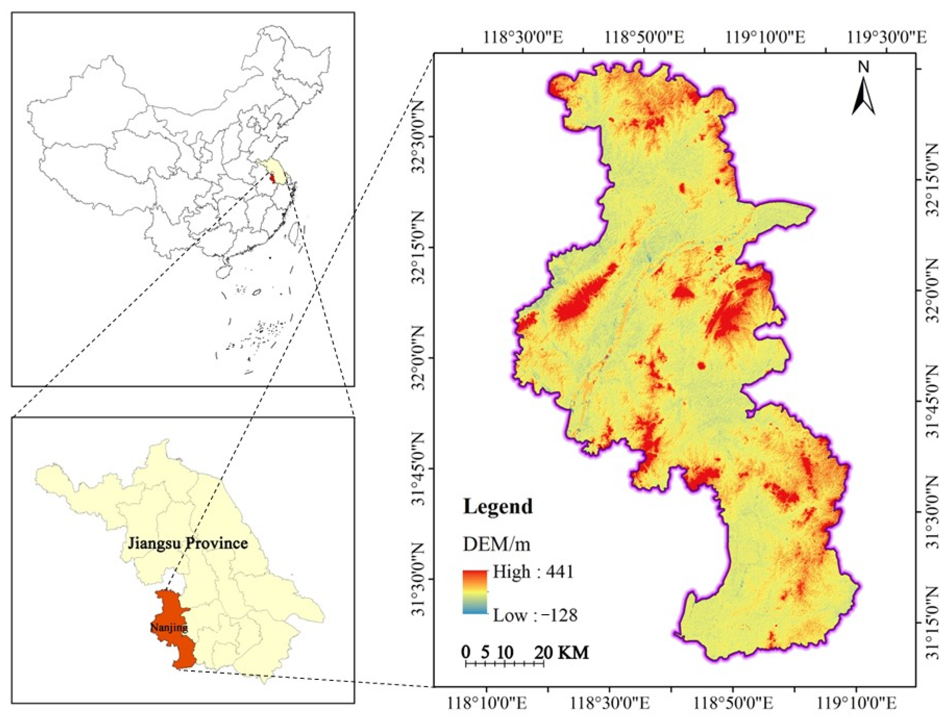
Nanjing, a city in eastern China, southwestern Jiangsu Province, along the lower reaches of the Yangtze River, is a core city of the Yangtze River Delta, with the geographical coordinates of 31°14′–32°37′ N and 118°22′–119°14′ E (see Figure 1). The city straddles the Yangtze River, connecting the Jianghuai Plain to the north and Yangtze River Delta to the east, with a maximum horizontal distance of approximately 70 km from east to west and 150 km from north to south. The city has a long north–south and narrow east–west plan, covering an area of 6587 km². Nanjing has experienced a high level of urbanization and rapid economic development, which has led to dramatic changes in land use types and an uneven land use structure conflicting with ecosystem gradually. This study analyzed whether there was a spatial correlation between the landscape pattern index, which characterized land use patterns, and ESV in Nanjing and, if so, further explored the impact of changes in land use patterns on the ESV.

2.2. Data Sources

Land use data in this study were obtained from the National Earth System Science Data Center (http://www.geodata.cn/, accessed on 10 February 2022) and the Data Sharing and Service Portal (https://data.casearth.cn/, accessed on 10 February 2022) for the global 30 m land cover dataset for 2010, 2015, and 2020 [23,24,25,26]. The crop sown area was obtained from the Nanjing Statistical Yearbook 2011–2019. The average net profit per unit area of crops came from the National Compilation of Information on the Costs and Benefits of Agricultural Products (2011–2019). Chinese net primary productivity (NPP), annual precipitation interpolation, and soil erosion spatial distribution data were obtained from the Resource and Environment Science and Data Center (https://www.resdc.cn/, accessed on 18 February 2022).

2.3. Research Methods

2.3.1. Landscape Pattern Index

The landscape pattern index, based on land use/cover maps, is an important method for the analysis of spatial landscape patterns, making it possible to measure the interconnection of ecological processes and spatial patterns [27]. Landscape spatial pattern refers to the spatial configuration of landscape patches of varying sizes and shapes, and is an expression of landscape heterogeneity, whereas landscape indices can highly condense landscape pattern information, reflecting certain aspects of composition and spatial configuration [28,29,30].

Landscape indices that represent landscape patterns have ecological significance and each has differing emphasis and relevance [28,31]. To comprehensively reflect the overall land use pattern of the study area and reduce information redundancy, indicators with holistic characteristic were used to describe the spatial structure of land use patterns in Nanjing, considering the characteristics of the study area and referring to existing studies [32]. Using Fragstats v4.2.1 (produced by McGarigal, K., Cushman, S.A., and Ene, E., Boston, UK), at the landscape level, patch density (PD), largest patch index (LPI), contagion index (CONTAG), Shannon diversity index (SHDI), splitting index (SPLIT), and Shannon evenness index (SHEI) were selected for structural feature index calculations (see

Table 1. Landscape pattern indices and their ecological implications [32].

Landscape Pattern Indices	Ecological Implications
Patch Density (PD)	Reflects the number of all types of landscape patches within a unit area of landscape. Higher PD values indicate a more fragmented landscape.
Largest Patch Index (LPI)	Reflects the dominant type in a landscape area and characterizes the proportion of the largest patches of a given type to the area of the entire landscape region. Its value entangles the landscape of the dominant species, the rich inner species, and other ecological characteristics.
Contagion Index (CONTAG)	Reflects the degree of aggregation or extension trend of different patch types in the landscape. Smaller CONTAG values indicate the presence of many small patches in the landscape: a dense pattern with multiple elements. When the value is closer to 100, it indicates the presence of dominant patchwork types with very high connectivity in the landscape and a good degree of connectedness.
Splitting Index (SPLIT)	Reflects the fragmentation of the landscape area. The complexity of landscape spatial structure reflects the degree of human disturbance to landscape to a certain extent. In general, the greater the degree of separation, the greater the human impact on the ecosystem.
Shannon Diversity Index (SHDI)	Reflects the diversity of regional landscape types. An SHDI value of 0 indicates that the entire regional landscape consists of only one patch. The higher the SHDI value, the higher the level of landscape heterogeneity, and the more patch types or the fragmentation of the patches in the landscape.
Shannon Evenness Index (SHEI)	Reflects the evenness of patch type distribution in the landscape area. The SHEI upper bound is 1, which indicates that there are no dominant types in the landscape and all kinds of patches are evenly distributed in the landscape and can reflect the maximum diversity of the given landscape richness.

for specific ecological implications) to obtain results on the evolution of the spatial pattern.

2.3.2. Equivalence Factor Method

In this study, a method concerning the value equivalent factor per unit area (hereafter referred to as the equivalence factor method) was used, which is based on differentiating between types of ecosystem services functions, constructing value equivalents for various service functions of different types of ecosystems based on quantifiable criteria, and then assessing them in relation to the distribution area of the ecosystem [33]. The equivalence factor method is intuitive, easy to use, requires fewer data, and is suitable for the valuation of ecosystem services on regional and global scales [33,34,35].

Value of a Standard Unit of ESV Equivalent Factor

One standard unit of ESV equivalent factor (hereafter referred to as the standard equivalent) is the economic value of the annual natural food production of 1 ha of nationally averaged yielding farmland, which serves to characterize and quantify the potential capacity of different types of ecosystems to contribute to ecological service functions [36]. In this study, the net profit-weighted averages of the three major crops of rice, wheat, and soybeans in Nanjing from 2010 to 2018 were used to obtain the standard equivalent factor economic value, referring to the treatment by Xie [33]. The calculation formula is as follows:

$$\mathrm{D}=\frac{1}{9}{{\displaystyle \sum }}_{\mathrm{i}=1}^9\left({\mathrm{S}}_{\mathrm{i}}^{\mathrm{r}}{ \times \mathrm{F}}_{\mathrm{i}}^{\mathrm{r}}{+\mathrm{S}}_{\mathrm{i}}^{\mathrm{w}}{ \times \mathrm{F}}_{\mathrm{i}}^{\mathrm{w}}{+\mathrm{S}}_{\mathrm{i}}^{\mathrm{b}}{ \times \mathrm{F}}_{\mathrm{i}}^{\mathrm{b}}\right)$$

(1)

where D is one standard equivalent factor of ESV (USD/ha); ${\mathrm{S}}_{\mathrm{i}}^{\mathrm{r}}$, ${\mathrm{S}}_{\mathrm{i}}^{\mathrm{w}}$, and ${\mathrm{S}}_{\mathrm{i}}^{\mathrm{b}}$ are the proportions (in %) of the sown area of rice, wheat, and soybean to the sown area of the three crops in year i, respectively; and ${\mathrm{F}}_{\mathrm{i}}^{\mathrm{r}}, {\mathrm{F}}_{\mathrm{i}}^{\mathrm{w}}$, and ${\mathrm{F}}_{\mathrm{i}}^{\mathrm{b}}$ are the average net profit per unit area for rice, wheat, and soybean in year i, respectively. The final D value was 299.01 USD/ha.

Value Coefficient of Ecosystem Services Function per Unit Area

The base equivalence of the ESV per unit area refers to the average annual value of each type of service function per unit area for different types of ecosystems (hereinafter referred to as the base equivalence). This study used the national base equivalence scale proposed by Xie [33] as a reference. Simultaneously, to reflect the internal heterogeneity of the ecological function value equivalence factors of the same ecosystem type, the NPP regulator (to correct the service functions of food production, raw materials, gas regulation, climate regulation, environmental purification, nutrient cycling, biodiversity, and aesthetic landscape), the precipitation regulator (to correct the service functions of water supply and hydrological regulation), and soil conservation factor (to correct the service functions of soil conservation) were used to correct the Nanjing ESV equivalence factors. The correction factor is calculated as follows [37]:

$${\mathrm{V}}_{\mathrm{if}}{=\mathrm{V}}_{\mathrm{f}}{ \times \mathrm{E}}_{\mathrm{in}}$$

(2)

where ${\mathrm{V}}_{\mathrm{if}}$ is the equivalent factor of the f-type service function in region i; ${\mathrm{V}}_{\mathrm{f}}$ is the national average equivalent factor of the f-type service function of the ecosystem; ${\mathrm{E}}_{\mathrm{in}}$ is the spatial regulating factor for the three service functions of the ecosystem in region i. Category 1 ecosystem services are food production, raw materials, gas regulation, climate regulation, environmental purification, nutrient cycling, biodiversity, and aesthetic landscape. These service functions positively correlate with biomass in general. Category 2 ecosystem services are water supply and hydrological regulation, which are related to precipitation change. Finally, category 3 ecosystem services include soil conservation.

${\mathrm{E}}_{\mathrm{i}1}$ is the regulator of category 1 ecosystem services functions:

$${\mathrm{E}}_{\mathrm{i}1}{=\mathrm{NPP}}_{\mathrm{i}}/\overline{\mathrm{NPP}}$$

(3)

where ${\mathrm{NPP}}_{\mathrm{I}}$ is the annual average NPP in area i of Nanjing (t/ha), and $\overline{\mathrm{NPP}}$ is the average annual NPP per unit area nationwide (t/ha).

${\mathrm{E}}_{\mathrm{i}2}$ is the regulator of category 2 ecosystem services functions:

$${\mathrm{E}}_{\mathrm{i}2}{=\mathrm{P}}_{\mathrm{i}}/\overline{\mathrm{P}}$$

(4)

where ${\mathrm{P}}_{\mathrm{I}}$ is the annual average precipitation per unit area in area i of Nanjing (mm/ha), and $\overline{\mathrm{P}}$ is the national average annual precipitation per unit area (mm/ha).

${\mathrm{E}}_{\mathrm{i}3}$ is the regulator of category 3 ecosystem services functions:

$${\mathrm{E}}_{\mathrm{i}3}{=\mathrm{S}}_{\mathrm{i}}/\overline{\mathrm{S}} \mathrm{or} {\mathrm{E}}_{\mathrm{i}3}{=\mathrm{e}}_{\mathrm{i}}/\overline{\mathrm{e}}$$

(5)

where ${\mathrm{S}}_{\mathrm{i}}$ is the average annual soil retention simulation per unit area in area i (t/ha); $\overline{\mathrm{S}}$ is the national soil retention simulation per unit area (t/ha); ${\mathrm{e}}_{\mathrm{i}}$ is the average soil erosion modulus in area i (t/km²/a); $\overline{\mathrm{e}}$ is the national average soil erosion modulus (t/km²/a). As the regional soil conservation function is governed by the amount of natural soil erosion in the area, the spatial distribution data of soil erosion from the Resource and Environment Science and Data Center was used in this study to obtain the regulating factors of the soil conservation function.

The value coefficient of the ecosystem services function per unit area is then calculated by:

$${\mathrm{C}}_{\mathrm{if}}{=\mathrm{D} \times \mathrm{V}}_{\mathrm{if}}$$

(6)

where ${\mathrm{C}}_{\mathrm{if}}$ is the coefficient of the ESV category f per unit area in area i, which is the product of the standard equivalent $\mathrm{D}$ and base equivalent ${\mathrm{V}}_{\mathrm{if}}$.

2.3.3. Moving Window Approach

To improve precision, considering the total ESV and raster scale of land cover data, a square window with a side length of 300 m was set-up using the Fragstats moving window method. The landscape pattern index of each window was extracted and, finally, the raster images of the landscape pattern index of 2010, 2015, and 2020 were obtained.

In ArcGIS 10.5 (produced by Environmental Systems Research Institute, Redlands, CA, USA), the landscape pattern index and total ESV were raster processed to form 1 × 1 km grid units, and the raster data were normalized by min–max normalization using the formula:

$${\mathrm{x}}_{\mathrm{norm}}=\frac{{\mathrm{x} - \mathrm{x}}_{\min }}{{\mathrm{x}}_{\max }{- \mathrm{x}}_{\min }}$$

(7)

where ${\mathrm{x}}_{\mathrm{norm}}$ is the normalized value of the landscape pattern index or total ESV; $\mathrm{x}$ is the value of the landscape pattern index or total ESV for a given grid; ${\mathrm{x}}_{\min }$ is the minimum value of a category of landscape pattern index or total ESV in the study area grid; ${\mathrm{x}}_{\max }$ is the maximum value of a category of landscape pattern index or total ESV in the study area grid.

2.3.4. Spatial Autocorrelation

Univariate Spatial Autocorrelation

Moran’s I could be used to test for the presence of spatial autocorrelation against the null hypothesis of no autocorrelation [38]; thus, this study chose the autocorrelation graph of Moran’s I for analysis. The formula is as follows:

$$\mathrm{I}=\frac{\mathrm{n}{\displaystyle \sum _{\mathrm{i}=1}^{\mathrm{n}}}{\displaystyle \sum _{\mathrm{j}\ne \mathrm{i}}^{\mathrm{n}}}{\mathrm{w}}_{\mathrm{ij}}\left({\mathrm{x}}_{\mathrm{i}}-\overline{\mathrm{x}}\right)\left({\mathrm{x}}_{\mathrm{j}}-\overline{\mathrm{x}}\right)}{\left({\displaystyle \sum _{\mathrm{i}=1}^{\mathrm{n}}}{\displaystyle \sum _{\mathrm{j}\ne 1}^{\mathrm{n}}}{\mathrm{w}}_{\mathrm{ij}}\right){\displaystyle \sum _{\mathrm{i}=1}^{\mathrm{n}}}{\left({\mathrm{x}}_{\mathrm{j}}-\overline{\mathrm{x}}\right)}^2}$$

(8)

where $\mathrm{n}$ is the number of spatial units (i.e., 6972 grid units); ${\mathrm{x}}_{\mathrm{i}}$ and ${\mathrm{x}}_{\mathrm{j}}$ are the values of the landscape pattern index or ESV of grid units i and j; $\overline{\mathrm{x}}$ is the mean value of the landscape pattern index or the total ESV for all grid units; ${\mathrm{w}}_{\mathrm{ij}}$ is the space weight matrix. Moran’s I ϵ (−1,1). When I > 0, the landscape pattern index or total ESV is positively spatially correlated, showing aggregated distribution characteristics. When I ≈ 0, there is no evidence of spatial autocorrelation, suggesting the hypothesis that the spatial distribution of landscape pattern indexes or ESV is purely random. When I < 0, the landscape pattern index or total ESV is negatively spatially correlated, showing discrete distribution characteristics.

Bivariate Spatial Autocorrelation

Bivariate spatial autocorrelation analysis, proposed by Anselin [39], can reveal correlations between spatial variables and other variables in neighboring regions. This method was applied here to verify whether there was a spatial correlation between a single landscape pattern index and ESV and to prepare for the next step in the spatial regression, with Equations (9) and (10) [40]:

$${\mathrm{I}}_{\mathrm{lm}}^{\mathrm{p}}{=\mathrm{Z}}_{\mathrm{l}}^{\mathrm{p}}·{{\displaystyle \sum }}_{\mathrm{q}=1}^{\mathrm{n}}{\mathrm{W}}_{\mathrm{pq}}{·\mathrm{Z}}_{\mathrm{m}}^{\mathrm{q}}$$

(9)

$${\mathrm{Z}}_{\mathrm{l}}^{\mathrm{p}}=\frac{{\mathrm{X}}_{\mathrm{l}}^{\mathrm{p}}-\overline{{\mathrm{X}}_{\mathrm{l}}}}{{\mathsf{\sigma }}_{\mathrm{l}}}, {\mathrm{Z}}_{\mathrm{m}}^{\mathrm{q}}=\frac{{\mathrm{X}}_{\mathrm{m}}^{\mathrm{q}}-\overline{{\mathrm{X}}_{\mathrm{m}}}}{{\mathsf{\sigma }}_{\mathrm{m}}}$$

(10)

where ${\mathrm{I}}_{\mathrm{lm}}^{\mathrm{p}}$ is the Moran coefficient; ${\mathrm{X}}_{\mathrm{l}}^{\mathrm{p}}$ is the total ESV of the grid unit p; ${\mathrm{X}}_{\mathrm{m}}^{\mathrm{q}}$ is the value of the landscape pattern index for grid unit q; $\overline{{\mathrm{X}}_{\mathrm{l}}}$ and ${\mathsf{\sigma }}_{\mathrm{l}}$ are the mean and variance of the total ESV; $\overline{{\mathrm{X}}_{\mathrm{m}}}$ and ${\mathsf{\sigma }}_{\mathrm{m}}$ are the mean and variance of the landscape pattern index, respectively.

2.3.5. Spatial Autoregression

If there is a strong spatial dependence of variables in a geographical phenomenon, contrary to the classical statistical assumption of sample independence, spatial interactions must be incorporated into the classical regression model in the form of a spatial weight matrix for spatial autoregressive analysis. According to the spatial correlation between the independent and dependent variables, Anselin [39] proposed a general form of the spatial regression equation:

$$\{\begin{array}{l}\mathrm{y}=\mathsf{\rho }{\mathrm{W}}_1\mathrm{y}+\mathsf{\beta }\mathrm{X}+\mathsf{\mu }\\ \mathsf{\mu }=\mathsf{\lambda }{\mathrm{W}}_2\mu +\mathsf{\epsilon }\\ \mathsf{\epsilon }:\mathrm{N}\left(0, {\mathsf{\delta }}^2\mathrm{I}\right)\end{array}$$

(11)

where $\mathrm{y}$ refers to ESV; $\mathrm{X}$ refers to landscape pattern index (i.e., PD, CONTAG, SPLIT, LPI, and SHEI); $\mathsf{\beta }$ is the regression coefficient; $\mathsf{\mu }$ is the random error term; $\mathsf{\epsilon }$ is the random error obeying a mean of 0 and a variance of ${\mathsf{\delta }}^2$; ${\mathrm{W}}_1$ and ${\mathrm{W}}_2$ are the weight matrices of ESV and residual; $\mathsf{\rho }$ is the coefficient of spatial lag term ${\mathrm{W}}_1\mathrm{y}$; $\mathsf{\lambda }$ is the coefficient of spatial error term ${\mathrm{W}}_2\mathsf{\mu }$. When the different parameter vectors are set to zero, four different spatial model structures can be generated [41]. Because the effect of independent variables on dependent variables is not considered in the first-order spatial autoregressive model (i.e., $\mathsf{\rho }$ ≠ 0, $\mathsf{\beta }$ = $\mathsf{\lambda }$ = 0), this study only considered the ordinary linear regression (OLS), spatial lag model (SLM), and spatial error model (SEM), with β ≠ 0, as shown in

Table 2. Spatial autoregressive models.

Model	Forming Conditions	Significance
Ordinary Linear Regression (OLS)	$\mathsf{\rho }=0$, $\mathsf{\lambda }=0$	The model generally assumes that observations are independent of each other and not influenced by other factors and does not consider spatial variability between regions.
Spatial Lag Model (SLM)	$\mathsf{\rho }\ne 0$, $\mathsf{\lambda }=0$	The model considers the spatial correlation of the dependent variable, i.e., the dependent variable in a given spatial region is not only related to the independent variable in the same region but also to the dependent variable in neighboring regions.
Spatial Error Model (SEM)	$\mathsf{\rho }=0$, $\mathsf{\lambda }\ne 0$	The model does not consider the spatial correlation of the dependent variable but only the spatial autocorrelation of the independent variable, i.e., the dependent variable in a given spatial region is related to the independent variable in the same region, the independent variable in neighboring regions, and the dependent variable.

.

The classical goodness-of-fit R² can be used to compare the OLS model; however, in the case of spatial autoregressive models, each model’s goodness-of-fit must be compared using a combination of the maximum likelihood logarithm (LIK), Akaike information criterion (AIC), and Schwartz criterion (SC). If the LIK of the model is larger and the AIC and SC are smaller, the model’s goodness-of-fit will be better.

2.4. Research Framework

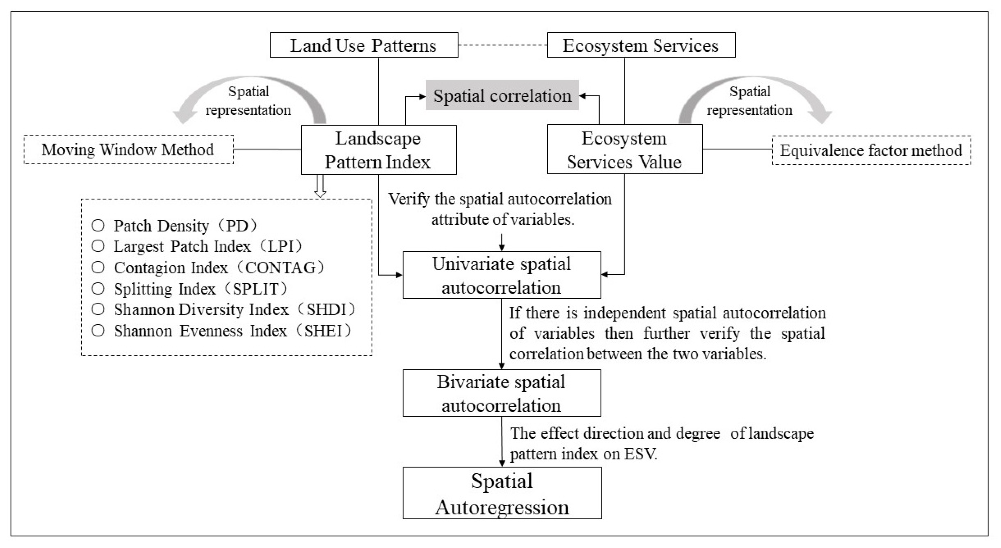
The technical framework of this study is illustrated in Figure 2. The landscape pattern index was represented using the moving window method, and the ESV was represented using the equivalence factor method. If the variables were spatially autocorrelated, the effect degree of the landscape pattern index on the ESV would be analyzed by spatial autoregression. This study attempted to explore the response of ecosystem services triggered by changes in land spatial structure due to the fact of urban land stress through a spatial analysis approach.

3. Results

3.1. Evolution of Land Use Patterns

The results of the landscape pattern indices selected for the study were calculated using Fragstats, as shown in Figure 3, and spatially characterized by differentiation at the spatial unit scale, as shown in Figure S1. PD reflects the overall landscape fragmentation, with a higher patch density, indicating a more fragmented landscape. Compared to 2010, PD decreased in 2020, indicating that the regional landscape was less resilient to external disturbance. The LPI reflects the degree of landscape-dominant species. Comparing three years, LPI was the highest in 2010, showing a better patch integrity. Its rose from 2015 to 2020, indicating that dominant species recovered again. CONTAG reflects the degree of clustering of the different patch types. The CONTAG first increased but then decreased from 2010 to 2020, and the patch connectivity was the lowest in 2020 and highest in 2015, indicating a decreasing trend in patch connectivity and a dense distribution of elements in the landscape. The SPLIT reflects the degree of landscape patch segmentation. The degree of disturbance in the first 5 years was higher than that in the last 5 years and the degree of separation in 2020 was higher than that in 2010. The SHDI reflects landscape heterogeneity and type richness. The SHDI increased over the 10 year period, with the average change decreasing from 0.0835 to 0.0074, indicating increasing landscape heterogeneity, diversification of landscape types, complexity of each landscape type, and a tendency to weaken. The SHEI reflects the evenness of patches in the landscape area. The increase in SHEI in the first 5 years was smaller than that in the last 5 years, indicating that landscape evenness increased.

In general, during the 10 year period, the land patch in Nanjing had a decreased density, with a tendency towards clustering and a weakening of the dominant patch type. The connectivity level of the patches decreased, and the distribution was even, indicating an increased landscape heterogeneity.

3.2. Spatial–Temporal Change of ESV

3.2.1. Coefficient of ESV per Unit Area in Nanjing

Based on the national-scale base equivalence table proposed by Xie [33], a modified equivalence factor table was obtained using three types of moderating factors, as shown in

Table 3. Modified equivalent factors for ESV per unit area in Nanjing.

Classification of Ecosystems		Provision			Regulation				Support			Culture
Grade 1 Classification	Grade 2 Classification	Food Production	Raw Materials	Water Supply	Gas Regulation	Climate Regulation	Environmental Purification	Hydrological Regulation	Soil Conservation	Nutrient Cycling	Biodiversity	Aesthetic Landscape
Cropland	Dry land	1.11	0.52	0.05	0.88	0.47	0.13	0.63	0.63	0.16	0.17	0.08
	Paddy field	1.78	0.12	−6.12	1.45	0.75	0.22	6.33	0.01	0.25	0.27	0.12
Forest	Needle-leaved forest	0.29	0.68	0.63	2.23	6.64	1.95	7.77	1.27	0.21	2.46	1.07
	Mixed leaf forest	0.41	0.93	0.86	3.08	9.20	2.60	8.17	1.76	0.29	3.40	1.49
	Broad-leaved forest	0.38	0.86	0.79	2.84	8.51	2.53	11.03	1.63	0.26	3.15	1.39
	Shrubland	0.25	0.56	0.51	1.85	5.54	1.68	7.80	1.06	0.17	2.06	0.90
Grassland	Grassland	0.13	0.18	0.19	0.67	1.75	0.58	2.28	0.38	0.07	0.73	0.33
	Scrub	0.50	0.73	0.72	2.58	6.82	2.25	8.89	1.48	0.24	2.85	1.26
	Meadow	0.29	0.43	0.42	1.49	3.95	1.31	5.14	0.85	0.14	1.66	0.73
Wetland	Wetland	0.67	0.65	6.03	2.49	4.71	4.71	56.38	1.42	0.24	10.30	6.19
Desert	Desert	0.01	0.04	0.05	0.14	0.13	0.41	0.49	0.08	0.01	0.16	0.07
	Bare land	0.00	0.00	0.00	0.03	0.00	0.13	0.07	0.01	0.00	0.03	0.01
Water	Waterways	1.05	0.30	19.29	1.01	3.00	7.26	237.91	0.57	0.09	3.34	2.47
	Glacial snow	0.00	0.00	5.03	0.24	0.71	0.21	16.59	0.00	0.00	0.01	0.12

.

Based on the D-value and Table 3, the value coefficients of the ecosystem services functions in Nanjing can be obtained as shown in

Table 4. ESV coefficient per unit area in Nanjing. Unit: USD/ha.

Classification of Ecosystems		Provision			Regulation				Support			Culture
Grade 1 Classification	Grade 2 Classification	Food Production	Raw Materials	Water Supply	Gas Regulation	Climate Regulation	Environmental Purification	Hydrological Regulation	Soil Conservation	Nutrient Cycling	Biodiversity	Aesthetic Landscape
Cropland	Dry land	332.70	156.56	13.91	262.24	140.91	39.14	187.87	189.41	46.97	50.88	23.49
	Paddy field	532.32	35.23	−1829.96	434.47	223.10	66.54	1892.59	1.84	74.37	82.20	35.23
Forest	Needle-leaved forest	86.11	203.53	187.87	665.40	1984.45	583.20	2323.99	378.82	62.63	735.85	320.96
	Mixed leaf forest	121.34	277.90	257.45	919.81	2751.61	778.91	2442.28	525.94	86.11	1017.66	446.21
	Broad-leaved forest	113.51	258.33	236.57	849.36	2544.16	755.42	3298.12	487.32	78.28	943.30	414.89
	Shrubland	74.37	168.31	153.08	551.89	1655.66	501.00	2330.95	316.30	50.88	614.51	270.07
Grassland	Grassland	39.14	54.80	55.67	199.62	524.49	172.22	681.89	114.01	19.57	219.19	97.85
	Scrub	148.74	219.19	215.70	771.08	2039.24	673.22	2657.98	441.35	70.45	853.27	375.75
	Meadow	86.11	129.17	125.24	446.21	1182.06	391.41	1537.73	255.61	43.06	497.09	219.19
Wetland	Wetland	199.62	195.70	1802.14	743.68	1409.07	1409.07	16859.38	424.79	70.45	3080.39	1851.37
Desert	Desert	3.91	11.74	13.92	43.06	39.14	121.34	146.12	23.91	3.91	46.97	19.57
	Bare land	0.00	0.00	0.00	7.83	0.00	39.14	20.87	3.68	0.00	7.83	3.91
Water	Waterways	313.13	90.02	5768.23	301.38	896.33	2172.32	71139.20	171.02	27.40	998.09	739.76
	Glacial snow	0.00	0.00	1502.94	70.45	211.36	62.63	4961.10	0.00	0.00	3.91	35.23

.

3.2.2. Changes in ESV

Based on the scope of Nanjing City, 1 × 1 km grid cells were selected as the scale of analysis, the ESV of grid cells in the study area was calculated, and their spatial distribution results were analyzed as shown in Figure 4. From 2010 to 2020, the ESV of the Nanjing grid cell changed significantly, and the scale and ductility of ESV high-value areas decreased. In 2020, the high ESV concentration areas were the Hewangba Reservoir, Jinniu Lake, and Shanhu Reservoirs in Liuhe District; Xuanwu Lake in Xuanwu District; Fangbian Reservoir and Zhongshan Reservoir in Lishui District; Gucheng Lake in Gaochun District; Shijiu Lake in Lishui District; Gaochun District. In 2010, the Huaihe River system in the northern part of the city, the Chuhe River system in the northwestern part of the city, and the middle and upper reaches of the Yangtze River in the Nanjing section were high-concentration areas of ESV, which declined by varying degrees in 2015 and 2020. The main reason for this was that large-scale polder and construction land occupation caused water, forests, and unused land to decline, weakening the ecological value of the land. In 2015, the Huaiyang Mountains, represented by the Laoshan Forest Farm in the central part of Pukou District; the western part of the Ningzhen Mountains, represented by the Qinglong Mountains and Tangshan Mountains in the northeast of Jiangning District; the river systems, represented by the Lishui River and Jurong River in the south, formed large-scale concentrations of ESV. In 2020, the river systems of the Lishui River and Jurong River were seriously eroded by construction, and cropland and large areas of water disappeared, resulting in a significant decrease in the ESV.

3.3. Spatial Relationship between Land Use Pattern and ESV

3.3.1. Spatial Correlation between the Landscape Pattern Index and ESV

Univariate Spatial Autocorrelation Test

Moran’s I was used to test the global spatial autocorrelation for all panel data in GeoDa 1.18 (a software for raster data analysis, produced by Anselin, L., Ibnu, S. and Youngihn, K., Chicago, USA), and the results are shown in

Table 5. Univariate global spatial autocorrelation analysis of landscape pattern index and ESV.

Variable		Moran’s I
		2010	2015	2020
Landscape Pattern Index	PD	0.509 (82.5941) ***	0.513 (81.7584) ***	0.531 (85.553) ***
	CONTAG	−0.264 (−60.0069) ***	0.523 (85.1399) ***	0.452 (75.8241) ***
	SHDI	0.517 (81.9847) ***	0.514 (82.0632) ***	0.544 (87.5505) ***
	SPLIT	0.491 (79.6394) ***	0.461 (74.5429) ***	0.489 (78.4835) ***
	LPI	−0.388 (−80.2644) ***	0.425 (67.8931) ***	0.397 (62.8753) ***
	SHEI	0.456 (73.3209) ***	0.522 (83.1548) ***	0.522 (84.6176) ***
ESV	ESV_sum	0.712 (119.5558) ***	0.754 (125.7984) ***	0.714 (121.2497) ***

The values within parentheses are z-scores. *** p < 0.001.

. The table shows a significant spatial autocorrelation for all six landscape pattern indices and ESV in 2010, 2015, and 2020 (Moran’s I ≠ 0, and passes the randomization test at the 1% highly significant level, |z-score| > 2.58 with 999 permutations). Among them, the 3 year Moran’s I of PD and SHDI were greater than 0.5, which was more prominent in the landscape pattern index, and the Moran’s I of SHEI in 2015 and 2020 were both 0.522, showing strong spatial aggregation. Compared with the landscape pattern index, Moran’s I for ESV were all greater than 0.7, with more significant spatial autocorrelation and significant aggregation. Therefore, spatial interactions should be considered when exploring the correlations between variables.

Bivariate Spatial Autocorrelation

In GeoDa, ESV was used as the first variable and the landscape pattern indices (i.e., PD, CONTAG, SPLIT, LPI, and SHEI) were used as the second variables to analyze the spatial correlation between the two. To assess the degree of spatial autocorrelation between the variables, Moran’s I and local indicators of spatial association (LISA) were calculated and tested for the presence of aggregation and divergence against the null hypothesis of no autocorrelation; both resulted significant by means of a z-test at a level p < 0.05. The results are shown in Figure 5.

The Moran’s I of the bivariate spatial autocorrelation between ESV and each landscape pattern index demonstrated clear spatial correlation between different groups of variables. Except for SPLIT, where the correlation with ESV decreased, the absolute value of Moran’s I for the other five landscape pattern indices with ESV increased gradually over time, indicating an increasing correlation. CONTAG had the highest correlation with ESV and was spatially negative, and SHEI had a slightly lower correlation with ESV and was again spatially negative. The remaining four landscape pattern indices showed different positive and negative characteristics in relation to ESV, as the land use type shifted in different years. The LISA clustering distributions of PD, SHDI, SPLIT, and ESV were relatively complex and highly similar. There was some complementarity in the LISA clustering distribution maps between ESV-LPI and ESV-SHEI.

3.3.2. Effects of Land Use Pattern Change on ESV

Collinearity Diagnosis of Independent Variables

A preliminary diagnose of multicollinearity between the landscape pattern indices to explain ESV for each of the considered years was performed in the SPSS statistical package by calculating the variance inflation factor (VIF). Then, a variable selection procedure suggested dropping SHDI, and all of the VIF values resulted in less than the usual threshold of 10 [42] for the remaining independent variables (see

Table 6. Multicollinearity diagnosis (dependent variable: ESV).

Landscape Pattern Index	VIF
	2010	2015	2020
PD	6.100	5.544	7.227
CONTAG	3.030	2.065	2.163
SPLIT	7.557	6.745	8.373
LPI	3.463	2.596	2.369
SHEI	3.149	5.777	4.158

); hence, they can be safely considered in a multiple regression model of ESV for each year.

Degree of Influence Analysis

The impact of the land use pattern on ESV is influenced by a combination of factors, such as PD, LPI, and SPLIT. Therefore, using ArcGIS and GeoDa, this study presented OLS, SLM, and SEM with a concentrated likelihood function method and discussed the effect degree of different landscape pattern indexes on ESV, and the results are shown in

Table 7. Spatial autoregressive model parameters for ESV and the landscape pattern index.

Parameters		2010			2015			2020
		OLS	SLM	SEM	OLS	SLM	SEM	OLS	SLM	SEM
	R2	0.308	0.744	0.747	0.404	0.791	0.802	0.619	0.792	0.799
	LIK	2332.190	5322.370	5250.765	1979.080	5182.170	5225.839	5022.140	6864.820	6759.669
	AIC	−4652.380	−10,630.700	−10,489.500	−3946.150	−10,350.300	−10,439.700	−10,032.300	−13,715.600	−13,507.300
	SC	−4611.280	−10,582.800	−10,448.400	−3905.060	−10,302.400	−10,398.600	−9991.190	−13,667.700	−13,466.200
	Moran’s I (error)	0.553	0.014	−0.006	0.616	0.034	−0.019	0.403	0.056	−0.015
	ρ	—	0.825 (109.637) ***	—	—	0.809 (110.531) ***	—	—	0.667 (75.303) ***	—
	λ	—	—	0.883 (127.352) ***	—	—	0.884 (128.003) ***	—	—	0.835 (98.108) ***
β	PD	0.076 (2.324) *	0.037 (1.843) ’	0.021 (0.832)	0.186 (4.624) ***	0.022 (0.924)	−0.096 (−2.866) **	0.125 (5.220) ***	0.079 (4.469) ***	0.024 (1.177)
	CONTAG	−1.130 (−45.492) ***	−0.385 (−23.257) ***	−0.463 (−22.215) ***	−0.944 (−52.008) ***	−0.338 (−26.522) ***	−0.514 (−31.444) ***	−1.007 (−74.942) ***	−0.478 (−39.147) ***	−0.578 (−41.721) ***
	SPLIT	1.042 (19.373) ***	0.340 (10.229) ***	0.390 (9.956) ***	1.025 (11.962) ***	0.348 (6.832) ***	0.442 (7.500) ***	0.565 (16.725) ***	0.295 (11.630) ***	0.415 (14.719) ***
	LPI	1.012 (42.499) ***	0.396 (25.514) ***	0.448 (24.141) ***	0.801 (40.789) ***	0.366 (28.453) ***	0.511 (35.281) ***	0.832 (63.516) ***	0.428 (38.179) ***	0.518 (42.804) ***
	SHEI	−0.454 (−21.968) ***	−0.119 (−9.360) ***	−0.124 (−7.572) ***	−0.326 (−12.549) ***	−0.035 (−2.278) *	−0.003 (−0.186)	−0.352 (−23.630) ***	−0.171 (−15.061) ***	−0.224 (−17.048) ***
	Constant	0.005 (0.312)	−0.077 (−8.299) ***	0.017 (1.244)	0.062 (3.867) ***	−0.086 (−9.066) ***	0.016 (1.162)	0.040 (3.839) ***	−0.033 (−4.212) ***	0.031 (3.249) ***

The values within parentheses are t- or z-scores. *** p < 0.001, ** p < 0.01, * p < 0.05, and ’ p < 0.1.

.

First, we determined the unsuitability of the OLS model. The OLS model Moran’s I (error) values for 2010, 2015, and 2020, respectively, were 0.553, 0.616, and 0.403, indicating that OLS without consideration of spatial correlation could not effectively explain the relationship between variables. Second, the models were compared using the Lagrange multiplier term (LM) test. The OLS model was used to estimate the constrained model. Two LM test items, LMlag and LMErr, and their robust values, R-LMlag and R-LMerr, were highly significant (p < 0.001), indicating that both SLM and SEM could both explain the relationship between the landscape pattern index and ESV. Finally, compared with the OLS model, the LIK values of SLM (2010 and 2020) and SEM (2015) increased, the AIC and SC values decreased, and the Moran’s I value of the model residuals approached 0, which effectively reduced the model estimation error and better fitted the relationship among variables. Therefore, it is more reasonable to use SLM in 2010, SEM in 2015, and SLM in 2020 to analyze the spatial relationship between ESV and the landscape pattern index.

The model parameters are shown in Figure 6. From 2010 to 2020, the absolute values of the regression coefficients of LPI and CONTAG were higher than those of other pattern indices. The regression coefficient of LPI increased from 0.396 (2010) to 0.511 (2015) and finally decreased to 0.428 (2020). The regression coefficient of CONTAG decreased from −0.385 (2010) to −0.514 (2015) and finally increased to −0.478 (2020). The absolute values of the two coefficients still showed an overall increasing trend over time, indicating that the influence of LPI and CONTAG on ESV gradually increased and became dominant, with a significant positive effect of LPI on ESV and a significant negative effect of CONTAG. The regression coefficient of SPLIT increased from 0.34 (2010) to 0.442 (2015) and finally decreased to 0.295 (2020), with an overall decreasing trend. SPLIT was an index of landscape patterns that significantly affected ESV, in addition to LPI and CONTAG, with which it was spatially positively correlated. In addition, there was a significant negative correlation between SHEI and ESV in all three years, but with a weaker effect than LPI, CONTAG, and SPLIT. The regression coefficient of PD decreased from 0.037 (2010) to −0.096 (2015) and, finally, increased to 0.079 (2020). However, overall, the degree of the PD’s positive drive on ESV increased and had the weakest effect.

Therefore, combined with the changes in the landscape pattern index in Nanjing in 2010, 2015, and 2020, we know that while cultivating landscape agglomeration, the patch density within the cluster should be increased to form the dominant species landscape, maintaining a certain degree of separation between the clusters. Simultaneously, a landscape corridor should be established to ensure the connectivity of the inner and outer clusters. Constructing the complexity of the regional landscape spatial structure enhances resistance to the spread of disturbance. Thus, the land resources could exert a higher level of ecological value.

4. Discussion

4.1. ESV Response Induced by Land Spatial Structure Change

Rapid socioeconomic development and urbanization brings about huge land use transition, leading to regional socioeconomic and spatial reconfiguration [43]. Land use transition can be measured using the main forms of land use such as quantity, structure, and spatial patterns [44]. In conjunction with the results of previous studies, the negative impacts of spatial land change on regional ecosystem services can be constrained by controlling certain structural features of land use patterns during the transition process. Attention should be directed toward the cascade effect of land spatial ecological structure, and the degree of coordination between spatial structure and ecosystem services should be improved. In response to changes in the landscape pattern index in the study area, the overall SHEI for municipal sites showed a year-on-year increase in homogeneity, and the formation of dominant species in landscape areas was limited, which is not conducive to the promotion of ESV. Therefore, in the important ecological spatial structure, attention should be paid to cultivating natural ecological internal species in the region, restoring the degree of landscape dominance, reducing type uniformity in aggregated landscape clusters, and forming a scale concentration of ecological functions. In addition, among the five types of landscape pattern indices, CONTAG had the most significant negative effect on ESV, indicating that a dispersed land space structure is not conducive to ESV. This is consistent with the theory of agglomeration economies in urban economics, which states that the agglomeration effect of clustering space is a major driving force of urban growth [45]. At the urban scale, increased aggregation of land use patterns can facilitate the improved performance of regional ecosystem services. The search for the optimal layout of urban land use and long-term ESV benefits within the constraints of resources environment and economy society ensures the green and sustainable development of cities.

4.2. Urban Spatial Regulation in the Context of Ecosystem Services Trade-Offs

The spatial structure of urban and rural ecosystems based on land use influences the overall and local ecosystem services of the region, and there are constraints and interactions between the two. China’s rapid urbanization has led to a dramatic shift from natural or seminatural to construction land [46]. Large losses and high levels of ecological space fragmentation reduce ecosystem function and service delivery capacity, posing a range of ecological risks [47]. Over the study period, the landscape area in the study area shrunk, the distance between patches increased, and land use was diversified and homogeneous. Cropland area increased over the past decade to encircle other land types. The conversion of cropland to forests, grasslands, and lakes should be continued to enhance the total forests, grasslands, and water ecosystems. Additionally, efforts should be made to restore the ecology of the Yangtze River. Construction land is expanding in many ways, with the efficiency of urban construction land expansion gradually decreasing from the urban areas to the suburbs [48]. The population density of urban areas is higher than that of suburban areas. To prevent the contradiction between the population, resources, and the environment from escalating, construction land should be used with careful consideration. Through urban renewal and secondary development in the main urban areas, land use efficiency can be enhanced, and the encroachment of construction land on ecological land can be reduced. The future structure and pattern of land use should be determined in relation to its own functional positioning and comparative advantages and rules for the conversion of construction land under ecological constraints should be developed [49].

5. Conclusions

This research introduced the spatial autoregression model to analyze the spatial relationship between the landscape pattern index and ESV from 2010 to 2020 in Nanjing. The results showed: (1) There was a significant spatial aggregation of both the landscape pattern index and ESV in the study area with ESV being more significant, indicating that both had strong geospatial attributes. From 2010 to 2020, at the land use pattern level, the density of land patches in Nanjing decreased. Regional landscape showed a trend towards clustering, weakening of the dominant patch type, decreasing level of interpatch connectivity, homogenization of distribution, and increasing landscape heterogeneity. At the ESV level, the scale and extension of the high–medium ESV areas in Nanjing shrank. (2) There existed spatial correlations between land use patterns and ESV in geographical space. LPI and CONTAG played a dominant role in ESV, wherein LPI had a positive effect, and CONTAG had a negative effect. In 2015, the regression coefficients of landscape pattern indexes on ESV were all extreme values, perhaps because of the fact that the area of ecological land was the largest among all three years, making the effect of land use patterns on ESV obvious. (3) Ecological risk was aggravated by habitat destruction, and ecosystem services levels declined; therefore, it was necessary to realize the spatial regulation and value trade-off between urban structural elements or structural indices and ecosystem services.

The research results can serve as a reference for landscape form optimization aiming to realize a higher ecological value. Due to the limitation of available data, we only analyzed the relevant indicators for three years, and the time dimension can be added in future research. In order to determine how land use patterns affect ESV through spatial form, we should explore the impact mechanism and approach behind the statistical correlation between land use patterns and ESV, forming a complete reciprocal feedback mechanism between urban space and ecological environment.

References

- Meyer, W.B.; Turner, B.L., II. Changes in Land Use and Land Cover: A Global Perspective; Cambridge University Press: Cambridge, UK, 1994; p. 107. [Google Scholar]
- Daily, G.C. The value of nature and the nature of value. Science 2000, 289, 395–396. [Google Scholar] [CrossRef] [Green Version]
- Zhou, J.M.; Shen, R.F. Dictionary of Soil Science; Science Press: Beijing, China, 2013; p. 52. [Google Scholar]
- Lautenbach, S.; Kugel, C.; Lausch, A.; Seppelt, R. Analysis of historic changes in regional ecosystem service provisioning using land use data. Ecol. Indic. 2011, 11, 676–687. [Google Scholar] [CrossRef]
- Yuan, K.Y.; Li, F.; Yang, H.J.; Wang, Y.M. The influence of land use change on ecosystem service value in Shangzhou district. Int. J. Environ. Res. Public Health 2019, 16, 1321. [Google Scholar] [CrossRef] [PubMed] [Green Version]
- Wang, Y.Q.; Ma, J.M. Effects of land use change on ecosystem services value in Guangxi section of the Pearl River-West River Economic Belt at the county scale. Acta Ecol. Sin. 2020, 40, 7826–7839. [Google Scholar]
- Howarth, R.B.; Farber, S. Accounting for the value of ecosystem services. Ecol. Econ. 2002, 41, 421–429. [Google Scholar] [CrossRef]
- Egoh, B.; Rouget, M.; Reyers, B.; Knight, A.T.; Cowling, R.M.; Jaarsveld, A.S.; Welz, A. Integrating ecosystem services into conservation assessment: A review. Ecol. Econ. 2007, 63, 714–721. [Google Scholar] [CrossRef]
- Wainger, L.A.; King, D.M.; Mack, R.N.; Price, E.W.; Maslin, T. Can the concept of ecosystem services be practically applied to improve natural resource management decisions? Ecol. Econ. 2010, 69, 978–987. [Google Scholar] [CrossRef]
- Wang, X.L.; Bao, Y.H. Study on the methods of land use dynamic change research. Prog. Geogr. 1999, 1, 83–89. [Google Scholar]
- Zhang, H.; Zhang, B. Review on land use and land cover change models. J. Nat. Resour. 2005, 3, 422–431. [Google Scholar]
- Bai, W.Q.; Zhao, S.D. A comprehensive description of the models of land use and land cover change study. J. Nat. Resour. 1997, 2, 74–80. [Google Scholar]
- Future Earth. In Future Earth Initial Design: Report of the Transition Team; International Council for Science (ICSU): Paris, France, 2013.
- He, C.Y.; Zhang, J.X.; Liu, Z.F.; Huang, Q.X. Characteristics and progress of land use/cover change research during 1990–2018. Acta Geogr. Sin. 2021, 76, 2730–2748. [Google Scholar] [CrossRef]
- Liu, T.; Yang, X.J. Monitoring land changes in an urban area using satellite imagery, GIS and landscape metrics. Appl. Geogr. 2015, 56, 42–54. [Google Scholar] [CrossRef]
- Chen, X.; Wang, K.L.; Qi, X.K.; Li, H.B. Landscape pattern changes and evaluation of ecological service value of the Xiangjiang River watershed. Econ. Geogr. 2016, 36, 175–181. [Google Scholar]
- Liu, H.C.; Cui, M.H.; Li, Y.Y.; Li, M. The effect of land use change on ecosystem service value in the middle reaches of Fenhe River basin. J. Anhui Agric. Univ. 2021, 48, 635–640. [Google Scholar]
- Lei, H.; Wu, F.Q.; Xie, X.L. The spatial characteristics and relationships between landscape pattern and ecosystem service value along an urban-rural gradient in Xi’an city, China. Ecol. Indic. 2020, 108, 105720. [Google Scholar]
- Hu, J.L.; Zheng, W.J.; Wang, Y.X. Impact of landscape pattern evolution on ecosystem services value in Lijiang River basin. Landsc. Archit. 2020, 27, 64–70. [Google Scholar]
- Zheng, B.F.; Huang, Q.Y.; Tao, L.; Xie, Z.Y.; Ai, B.; Zhu, Y.H.; Zhu, J.Q. Landscape pattern change and its impacts on the ecosystem services value in southern Jiangxi Province. Acta Ecol. Sin. 2021, 41, 5940–5949. [Google Scholar]
- Gu, Z.Y.; Zhao, X.Q.; Gao, H.Y.; Xie, P.F. Change of landscape pattern and it’s evaluation of ecosystem services values in Lancang County. Ecol. Sci. 2016, 35, 143–153. [Google Scholar]
- Cressie, N.; Wikle, C.K. Statistics for Spatio-Temporal Data; Wiley: Hoboken, NJ, USA, 2011; p. 382. [Google Scholar]
- Gong, P.; Chen, B.; Li, X.; Liu, H. Mapping essential urban land use categories in China (EULUC-China): Preliminary results for 2018. Sci. Bull. 2020, 65, 182–187. [Google Scholar] [CrossRef] [Green Version]
- Zhang, X.; Liu, L.Y.; Chen, X.D.; Gao, Y.; Xie, S.; Mi, J. GLC_FCS30: Global land-cover product with fine classification system at 30 m using time-series Landsat imagery. Earth Syst. Sci. Data 2021, 13, 2753–2776. [Google Scholar] [CrossRef]
- Zhang, X.; Liu, L.Y.; Wu, C.S.; Chen, X.D.; Gao, Y.; Xie, S.; Zhang, B. Development of a global 30 m impervious surface map using multisource and multitemporal remote sensing datasets with the Google Earth Engine platform. Earth Syst. Sci. Data 2020, 12, 1625–1648. [Google Scholar] [CrossRef]
- Liu, L.Y.; Zhang, X.; Gao, Y.; Chen, X.D.; Xie, S.; Mi, J. Finer-Resolution Mapping of Global Land Cover: Recent Developments, Consistency Analysis, and Prospects. J. Remote Sens. 2021, 2021, 5289697. [Google Scholar] [CrossRef]
- Peng, J.; Wang, Y.L.; Zhang, Y.; Ye, M.T.; Wu, J.S. Research on the influence of land use classification on landscape metrics. Acta Geogr. Sin. 2006, 2, 157–168. [Google Scholar]
- Fu, B.J.; Chen, L.D.; Ma, K.M.; Wang, Y.L. Theory and Application of Landscape Ecology; Science Press: Beijing, China, 2001; p. 87. [Google Scholar]
- Wu, J.G. Landscape Ecology: Patten, Process, Scale and Hierarchy; Higher Education Press: Beijing, China, 2000; pp. 102–103. [Google Scholar]
- Zhao, R.F.; Zhou, H.R.; Xiao, D.N.; Qian, Y.B.; Zhou, K.F. Changes of wetland landscape pattern in the middle and lower reaches of the Tarim River. Acta Ecol. Sin. 2006, 10, 3470–3478. [Google Scholar]
- Hu, Y.X.; Pan, J.H. The stability of landscape pattern in Lanzhou, Gansu, China. J. Desert Res. 2016, 36, 556–563. [Google Scholar]
- Xiao, D.N.; Li, X.Z.; Gao, J.; Chang, Y.; Zhang, N.; Li, T.S. Landscape Ecology; Science Press: Beijing, China, 2010; p. 70. [Google Scholar]
- Xie, G.D.; Zhang, C.X.; Zhang, L.M.; Chen, W.H.; Li, S.M. Improvement of the evaluation method for ecosystem service value based on per unit area. J. Nat. Resour. 2015, 30, 1243–1254. [Google Scholar]
- Costanza, R.; Groot, R.; Sutton, P.; van der Ploeg, S.; Sharolyn, J.A.; Kubiszewski, I.; Farber, S.; Turner, R.K. Changes in the global value of ecosystem services. Glob. Environ. Chang. 2014, 26, 152–158. [Google Scholar] [CrossRef]
- Wang, W.J.; Guo, H.C.; Chuai, X.W.; Dai, C.; Lai, L.; Zhang, M. The impact of land use change on the temporospatial variations of ecosystems services value in China and an optimized land use solution. Environ. Sci. Policy 2014, 44, 62–72. [Google Scholar] [CrossRef]
- Xie, G.D.; Lu, C.X.; Leng, Y.F.; Zheng, D.; Li, S.C. Ecological assets valuation of the Tibetan Plateau. J. Nat. Resour. 2003, 18, 189–196. [Google Scholar]
- Li, Y.; Wang, Z.L.; Luo, J.M.; Liu, F.G.; Wang, X.H.; Li, Z.H. Reevaluation of ecosystem services value in the Nenjiang River Basin based on equivalent value factors. J. Sci. Teacher’s Coll. Univ. 2020, 40, 56–62. [Google Scholar]
- Chen, X.Y.; Lin, P. Spatial autocorrelation analysis on the distribution of Mangrove in China. J. East China Norm. Univ. 2000, 3, 104–109. [Google Scholar]
- Anselin, L. Spatial Econometrics: Methods and Models; Kluwer Academic Pulishers: Dordrecht, The Netherlands, 1988; p. 284. [Google Scholar]
- Yao, X.W.; Zeng, J.; Li, W.J. Spatial correlation characteristics of urbanization and land ecosystem service value in Wuhan Urban Agglomeration. Trans. Chin. Soc. Agric. Eng. 2015, 31, 249–256. [Google Scholar]
- Shen, Z.J.; Zeng, J.; Liang, C. Spatial relationship of greenspace landscape pattern with land surface temperature in three cities of southern Fujian. Chinese J. Ecol. 2020, 39, 1309–1317. [Google Scholar]
- Johnston, J.; Dinardo, J. Econometric Methods; McGraw-Hill: Singapore, 1984; p. 1. [Google Scholar]
- Ouyang, X.; Tang, L.S.; Wei, X.; Li, Y.H. Spatial interaction between urbanization and ecosystem services in Chinese urban agglomerations. Land Use Policy 2021, 109, 105587. [Google Scholar] [CrossRef]
- Long, H.; Kong, X.; Hu, S.; Li, Y. Land use transitions under rapid urbanization: A perspective from developing China. Land 2021, 10, 935. [Google Scholar] [CrossRef]
- Lu, Y.Y. The Economic Analysis on Urban Developing; SDX Joint Publishing Company: Shanghai, China, 2000; p. 63. [Google Scholar]
- Chen, M.; Liu, W.; Lu, D. Challenges and the way forward in China’s new-type urbanization. Land Use Policy 2016, 55, 334–339. [Google Scholar] [CrossRef]
- Wang, Y.C.; Shen, J.K.; Peng, Z.W.; Xiang, W.N. The optimization of green infrastructure ecosystem services adapted to urban growth. Chin. Landsc. Archit. 2018, 34, 45–49. [Google Scholar]
- Xu, G.; Pan, W.H.; Zhao, Y.; Han, X.M. Study on the expansion efficiency of urban construction land in Nanjing based on night light data. Henan Sci. Technol. 2019, 26, 90–95. [Google Scholar]
- Sun, W.; Liu, C.G.; Wang, S.N. Simulation research of urban development boundary based on ecological constraints: A case study of Nanjing. J. Nat. Resour. 2021, 36, 2913–2925. [Google Scholar] [CrossRef]
Figure 1.
Location of the study area.
Figure 2.
Technical framework.
Figure 3.
Landscape pattern index in Nanjing for three years. (a) PD values; (b) LPI values; (c) CONTAG values; (d) SPLIT values; (e) SHDI values; (f) SHEI values.
Figure 4.
Spatial distribution of grid unit ESV in Nanjing.
Figure 5.
Bivariate spatial autocorrelation analysis of ESV and the landscape pattern index. (a) cluster distribution of ESV and PD; (b) cluster distribution of ESV and LPI; (c) cluster distribution of ESV and CONTAG; (d) cluster distribution of ESV and SPLIT; (e) cluster distribution of ESV and SHDI; (f) cluster distribution of ESV and SHEI.
Figure 6.
Regression coefficient of the landscape pattern index.