An Integrated Turning Movements Estimation to Petri Net Based Road Traffic Modeling


AMIPS Research Team, Mohammadia School of Engineers, Mohammed V University in Rabat, Rabat 10000, Morocco
*
Author to whom correspondence should be addressed.
J. Sens. Actuator Netw. 2019, 8(3), 49; https://doi.org/10.3390/jsan8030049
Submission received: 9 August 2019
/
Revised: 13 September 2019
/
Accepted: 15 September 2019
/
Published: 18 September 2019
(This article belongs to the Special Issue Wireless Technologies Applied to Connected and Automated Vehicles)
Abstract
:The tremendous increase in the urban population highlights the need for more efficient transport systems and techniques to alleviate the increasing number of the resulting traffic-associated problems. Modeling and predicting road traffic flow are a critical part of intelligent transport systems (ITSs). Therefore, their accuracy and efficiency have a direct impact on the overall functioning. In this scope, a new approach for predicting the road traffic flow is proposed that combines the Petri nets model with a dynamic estimation of intersection turning movement counts to ensure a more accurate assessment of its performance. Thus, this manuscript extends our work by introducing a new feature, namely turning movement counts, to attain a better prediction of road traffic flow. A simulation study is conducted to get a better understanding of how predictive models perform in the context of estimating turning movements.
1. Introduction
The unprecedented growth of global urbanization has been accompanied by several critical issues such as air and noise pollution, insufficient public resource and services, traffic congestion, and excessive energy consumption. According to [1], 54% of the global population lives in urban land area, and it is projected to reach 70% by 2050. One of the most dramatic expressions of the urbanization phenomena can be found in [2], where the total economy-wide costs of congestion across four advanced economies, mainly the United States, the United Kingdom, France, and Germany, are estimated to soar from $200.7 billion in 2013 to $293.1 billion by 2030 (nearly a 50% increase from the 2013 gridlock costs). According to the same study, the number of hours wasted annually across those studied economies is predicted to result in a 6% increase in the average during the period 2013–2030; therefore, drivers are expected to waste an additional 6.8 hours in gridlock each year. Smart cities can play a key role in facing the urbanization pressures and their associated issues [3,4,5] where information and communication technologies (ICTs) can be used while balancing the needs of present and future generations with respect to economic, social, and environmental aspects.
2. Traffic Modeling
In this section, we present the traffic modeling, its benefits, its different types and classification, and the main modeling approaches. The primary objective of this section is twofold:
- Reviewing the existing research in road traffic flow modeling
- Defining the literature gaps for us to address within this work
2.1. Traffic Modeling and Its Benefits
“Data is the new oil” [6,7,8] is one of many statements that recognizes the rising importance of data and the urgent need to process it smartly, to extract useful knowledge from it, and more importantly, to build the most suitable data models.
Modeling data is playing a major role in urban knowledge discovery and improving the policies and management systems of urban networks. These networks include transportation, the Internet, telecommunication, water, electricity, etc. The primary goal of modeling data consists of properly describing the structure and the important features of the phenomenon or the system that generated the data. That is why the more the system is complex, the more powerful the data modeling must be and the more careful its process requires. Strictly related to transportation, since it is the main service that most other services within smart cities rely on, modeling road traffic flow is a key element as it has the potential to provide road users with vital information that can assist in making decisions, alleviating traffic congestion and improving the efficiency of transport system operations. Traffic road modeling is characterized by reproducing the traffic flow on the network based on the available observation data. As accurate, realistic, and real-time traffic modeling is, it has the potential to enable road users to make more informed travel decisions and assist the road administration to alleviate congestion and improve traffic management efficiency.
2.2. Traffic Modeling Approaches
With the development of traffic flow theories, three main categories of models were formed: a macroscopic approach that treats the traffic flow as a whole [9,10], the microscopic approach that considers individual vehicles and treats interactions between single vehicles [9,11,12], and the mesoscopic approach that combines the vehicle entities’ description with the macroscopic behavior [9,13].
Turning movement counts are critical and must be taken into consideration while modeling traffic since this information, on the one hand, is very important for investigating the effect of turning movement on the rest of traffic flow and for intersection behavior analysis and, on the other hand, can be utilized to improve the intersection operations and making decisions to solve traffic jam issues by means such as adaptive traffic signal control.
Several approaches have been introduced to study and model the traffic flow in the road network at different levels of detail. In this section, we give a brief review of the fundamental approaches addressing road traffic modeling:
- Continuum models treat the traffic flows as fluid streams where vehicles can be represented through average values and the discrete nature of the system or its individual components can be discarded. This category of models began with the first order (time and space derivatives are the order of one) LWR model [14,15] and then extended into higher order models thereafter. The common equation for all these models is the fundamental law of conservation that governs the traffic flow, speed, and density relationship. The LWR model, which was developed by Lighthill and Whitham, and Richards independently, is a continuous macroscopic representation of traffic variables. The LWR model was derived from the fluid mathematical field and conservation law theory and provides a description of the traffic flow by using the fluid dynamic differential equation:where represents the numbers of lanes in position x; represents the density per lane per kilometer at location x and time t; q is the flow per hour at location x and time t. In the LWR model, the speed and/or flow rate are considered as a function of density, which consists of the following equations:where and are respectively the maximal speed and the maximal density of a road.There is a basic assumption made about the LWR model of the dependence of the velocity on density alone. The main drawback of this dependency is that the model assumed the vehicle’s velocity is always in equilibrium, i.e., given a particular density, mainly when density tends to zero, the velocity will tend to infinity. Therefore, the model cannot describe observed behavior in light traffic and non-equilibrium traffic such as stop and go. On the other hand, the model does not deal with external conditions such as road conditions or vehicle behavior in front.
- A cellular automaton (CA) [16] is a simple, but powerful discrete microscopic model that is able to simulate many complex systems. In CA-models, the road traffic flow systems require a discretization in both time and space; time is discretized into time steps of equal duration, and the road is discretized into cells of equal size that are chosen sufficiently large such that a vehicle can drive at a velocity equal to one move to the next downstream cell during one time step. Each cell can either be empty or contain a vehicle.The brake-light Nagel–Schreckenberg (BL-NaSch) model [17,18] was proposed to represent a more complete description of the empirical observed phenomena in highway traffic using the cellular automaton. The BL-NaSchmodel combines velocity anticipation and a slow-to-start rule into the Nagel–Schreckenberg (NaSh) model [19]. In addition, a dynamical long-range interaction was introduced: drivers react to the braking of the leading vehicle indicated by the brake light. Therefore, the BL-NaSch model is considered as an extension of cellular automaton where the velocity and position of every car depend on the cars ahead. However, an important drawback of the BL-NaSch model is the computational requirements and the related costs and complexities, especially for large-scale road networks.
- The cell transmission model (CTM) was developed by Daganzo [20]. It was proposed for modeling the dynamic behavior of road traffic at the mesoscopic level. It adopts a discrete approach to predict traffic evolution in time and space. It consists of transforming the differential equations of the hydrodynamic model LWR [14,15] into simple differential equations. The CTMmodel divides the road network into small homogeneous and interconnected segments (called cells) and assumes piecewise linear relationships between flow and density in each cell. Hence, this model is able to describe and accurately capture the movement of propagation phenomena such as bottlenecks and the formation of shock waves in the traffic networks.Daganzo [20] showed that if the relationship between the traffic flow of vehicles (q) and the density (k) is of a triangular shape, then for a density k such that ( with the maximum density of a road), the flow is expressed as:where V,, W, and are constants designating, respectively, the free speed, maximum speed, the speed of propagation, and maximum density.CTM reveals several notable advantages at the mesoscopic level. The model is relatively simple and accurate enough to plan detailed analyses. Several studies have shown that the model enhances the realism in the representation of traffic for a variety of applications. However, several limitations of CTM must be overcome to meet the more complex needs of operational analysis.For example, the model in its original form requires the network to be divided into cells having a length corresponding to a clock tick (increment) of the simulation. This limitation may not be appropriate for large-scale networks because of possible geometric restrictions or inconsistencies with the division of network links in the cells and also the additional memory requirements by dividing the network into a large number of small cells. This limitation can lead to inefficient modeling of large-scale networks especially when combinations of small cells and various types of installations are used, such as highways and intersections of roads in the city.The original form of CTM [20,21] had a limited scope in the application to realistic networks, such as networks with traffic control devices (with traffic lights and intersections controlled, toll stations, etc.) that were either omitted or inadequately treated in the model.To our knowledge, most of the traffic models (including the aforementioned models) are performed with turning movement counts at intersections as a static input [22]. The fact is, however, that the real-time turning movement proportions are an important requirement for improving the road traffic modeling and increasing its relevance and efficiency. Turning movement counts are time-varying proportions that represent the intersection pattern during peak hours, morning middays and evenings, etc. Additionally, turning movement counts depend on the locations; at some locations, the traffic volume and then the turning movement may be higher than others, which leads to the guiding idea behind the contribution, in this article, which is that omitting modeling turning movement counts significantly decreases the validity of the real-world traffic modeling and its accuracy- and efficiency-related features.
The aforementioned models have limited scope in the application to realistic road networks and cannot provide acceptable accuracy for a certain number of road traffic rules, whih have been either omitted or insufficiently treated by the models such as priority roads, the “give way” rule at intersections, networks with controlled intersections, the congestion length in congested sections, etc.
Petri nets have become relevant due to their ability to represent complex systems and dealing with characteristics such as synchronization, parallelism, shared resources, etc. Interestingly, modeling the traffic flow by employing Petri nets has been shown to offer more adequate means for representing, analyzing, and understanding transportation systems since the behavior of traffic flow is considered as a phenomenon that combines synchronous, asynchronous, concurrent, parallel, continuous, and discrete aspects.
Accordingly, we presented in ref. [23] a traffic monitoring system that is based on Petri nets in order to deal with complex cases such as the “give way” rule, priority roads, etc., and address the issue of turning movement counts, and this will be discussed later in this work. Let us introduce a basic example to illustrate cases that are hard to be treated in the other models.
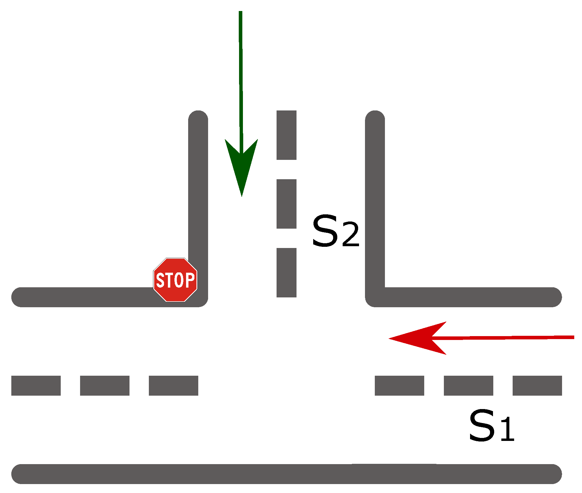
Example: In a T-intersection where a stop sign is installed for reminding drivers to stop and give way to any traffic in or approaching the intersection. This example is depicted in Figure 1.
In this example and other similar cases, the batch of vehicles and traffic evolution are not determined only by a fixed cycle time or flow rules, but also by uncontrollable events that may change dramatically the overall behavior of the traffic and consequently its different characteristics. In Figure 1, the behavior of the batch coming from depends completely on the batch from and can be accordingly divided into other batches due to the rule of stop and wait until the other batch has fully passed. These situations and others are not accurately modeled or are not taken into consideration by the aforementioned models.
Petri net modeling has been approached to study traffic flow at the macroscopic level and is used as a basis for the proposed work in this paper.
The rest of the paper is organized as follows. In Section 3, the related works are reviewed. The generalized nondeterministic batch Petri net is introduced in Section 4, while the most well-known estimation models are presented and discussed. The integrated turning movement count estimation models are simulated and compared in Section 5. Section 6 presents the results of the simulations described in Section 5. Conclusions are presented in Section 7.
3. Related Work
Turning movement counts (TMC) represent the counts of vehicle movements through an intersection over a given period of time. They are collected and used for a variety of purposes at both the planning level and the operational analysis level including intersection and traffic signal design, transport planning applications, etc.
The turning movement proportions estimation has been likened to the general problem of estimating a dynamic origin to destination matrix (OD matrix) in a small network.
Therefore, most of the proposed models make use of entry and exit counts at intersections [24,25,26,27]. For example, the aim of work [24] was to determine turning movement counts at signalized intersections based on entry/exit traffic volumes and signal phase information. The proposed method requires that flows at all entrance and exit lanes of an intersection be monitored.
In ref. [28], a vision-based vehicle tracking system was designed and used for estimating the turning movement counts, speed, and waiting time of vehicles at intersections. The idea was to use both background subtraction and feature extraction to detect and identify different moving vehicles in video surveillance and then match them from one frame to the next.
In ref. [29], an algorithm was given based on matrix algebra for determining turning movements at road intersections within which certain movements were prohibited. This was achieved by the development of mathematical models based on the continuity of flow and the fact that the available linearly independent equations were equal to the number of traffic streams. This led to reducing the number of data collectors needed for the turning movements at each link of a junction and the time required for the analysis of traffic survey data.
In ref. [27], Chen et al. proposed to make use of a nonlinear path flow estimator, originally developed to estimate path flows by using traffic counts from a subset of network links, to derive turning movements for the entire road network given some counts at selected intersections.
In their work [30], Lee et al. proposed a group-based method for lane-to-lane turning flow estimation in real time. In this regard, the authors considered firstly the rule-based approach through including information detected at downstream sensors such as departure and duration times, the occupancy time for downstream and upstream lanes, etc., then, a model-based approach by using regression logistic to improve turning movement predictions.
Some limitations of the proposed method are:
- Its inapplicability to medium and large scales as the error involving the random assignments will increase as the number of lanes increases;
- Its inability to be used in the cases where information of turning movement counts does not exist;
- The expensiveness of fully providing every intersection with sensors.
However, the paper [31] has to be mentioned. Jiao et al. [31] proposed a backpropagation Bayesian model combined with a Kalman filtering model to estimate the dynamic turning movement proportions at intersections. Except for the detected link counts, the Bayesian combined model did not take into consideration other parameters. As a result, traffic volumes for each lane of the entering approach were required, and therefore, the presence of detectors at the upstream lanes was mandatory.
4. Our Traffic Prediction System
The traffic model is the mathematical description of the traffic flow for characterizing and estimating the traffic state. It is an important part for solving the traffic problem and traffic management.
In this section, we discuss a road traffic prediction system based on wireless sensor networks (WSN) and its related overview; in this context, we propose an extended batch Petri net model in order to construct an explicit description of traffic flow evolution over space and time where the main contribution consists of taking into consideration the real-time estimation of turning movement counts. The Petri net modeling is adopted due to its analytical simplicity and capability of modelling different traffic flow states. Then, we present some predictive models in order to deal with the known turning movement counts at intersections.
4.1. Overview
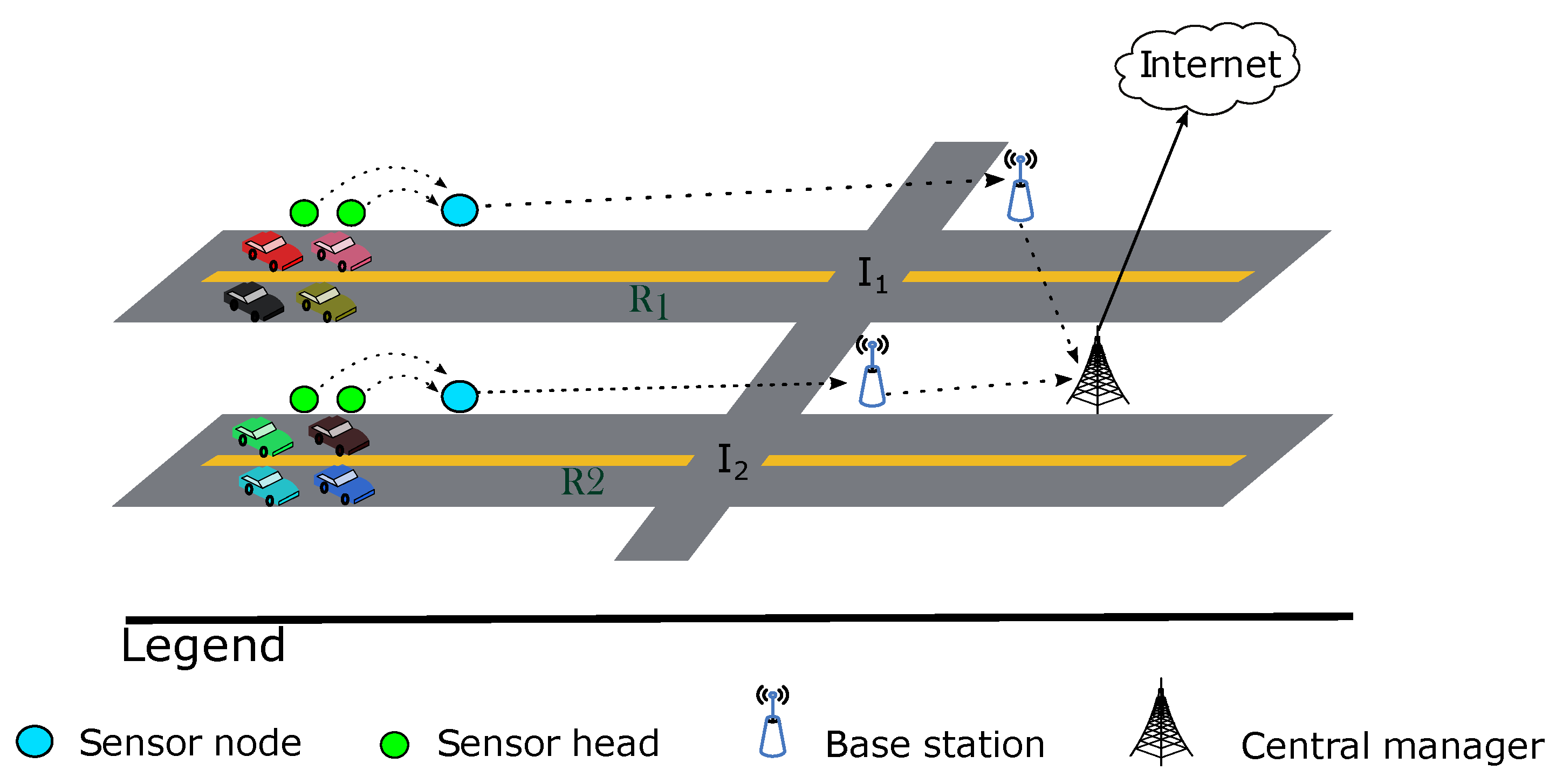
The WSN-based traffic management system (WTMS) collects data from different data sources including sensors, social media, calendar events, road works, and weather conditions, processes this data, provides input to a model, and creates a modeled state of the overall network, as well as the various regions of the network. The output of the model is transmitted to the administration for a decision-making process, and the system is able to notify users about administrators’ decisions.
The proposed system aims mainly at improving real-time traffic monitoring and prediction accuracy. More specifically, it (a) provides reliable road traffic flow estimation by taking into consideration different factors that affect the traffic (mainly six factors), (b) allows predicting traffic turning movement at forks and intersections, (c) is flexible to a high degree since it integrates different functionalities such as traffic forecasting, system administration, and control, and (d) seeks to be efficient since its design is distributed and can lead to non-crashing of the system in case of failures.
The WSN-based management system consists of eight basic components, which are the data acquisition component, data preprocessing component, data analysis component, visualization and reports component, system settings and administration component, traffic data repositories component, and finally, applications. All these components use the data communication component.
In the data acquisition component, the data can be gathered from sensors and also from the Internet, and it consists in particular of traffic flow average speed, volume, weather information, and other information. Through the data preprocessing component, the system can refine data by cleaning noise and duplications and imputing missing values. In the data analysis component, which is the main focus of this paper, the idea is to load and train collected data in order to build models, which represent knowledge of the recent road flow and the evolution of its traffic stream, which are used to provide better predictions.
4.2. Detailed System Workflow
Modeling and predicting traffic flow evolution comprise one of the most crucial challenges that must be tackled by any traffic management system.
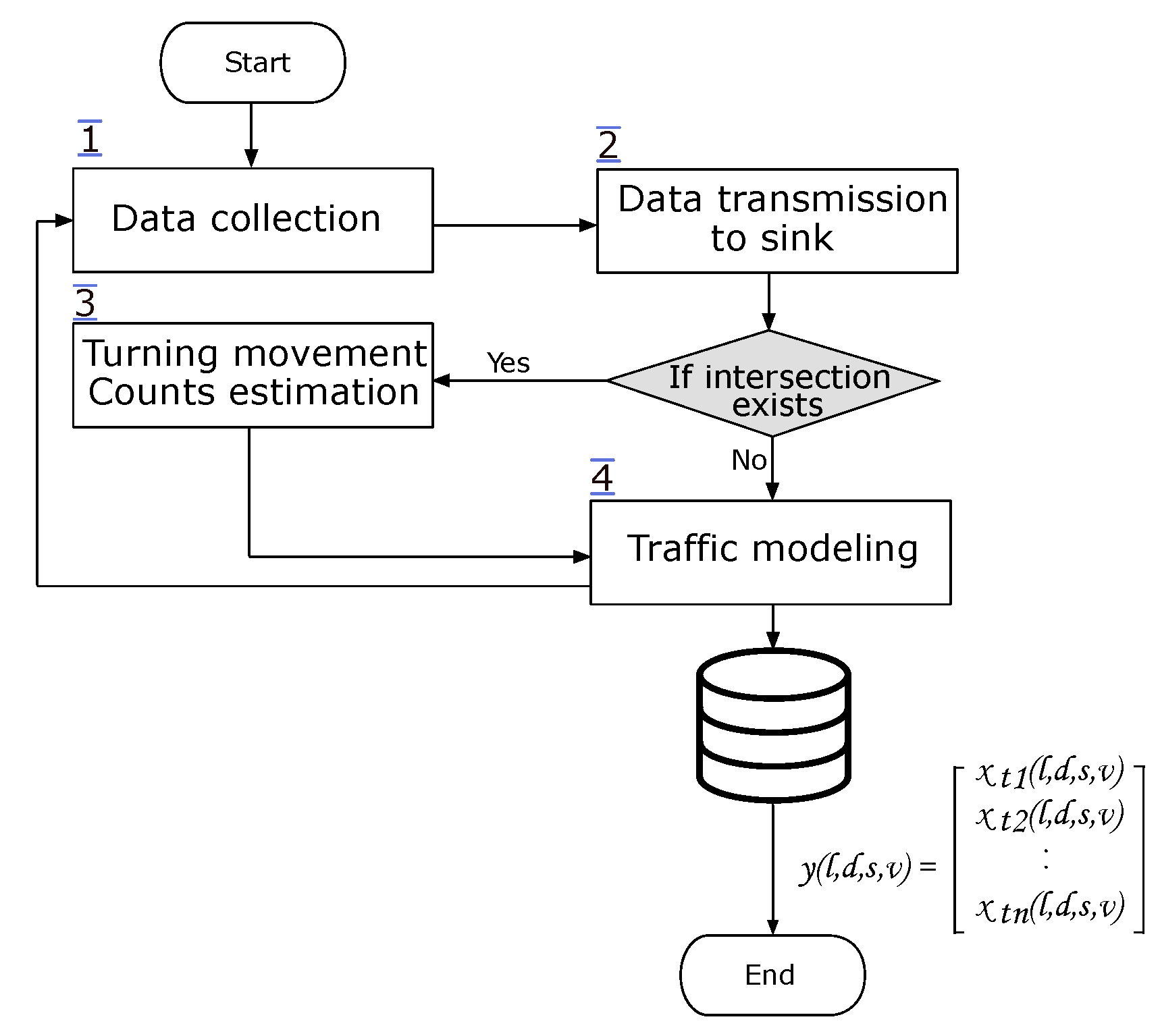
Figure 2 is a graphical representation depicting the proposed process by which the system predicts the evolution of traffic flow.
The main operational stages of the proposed process are: data collection, data transmission to the sink, turning movement estimation, and traffic modeling.
First of all, during data collection (Step 1), sensors, which are placed at entrances of roads, collect all the important data that is required for determining a batch of vehicles, its average speed, density, and length. Then, these parameters are transmit with the detection time to the neighboring sink (Step 2), where road traffic modeling will take place. During the modeling step (Step 4), if an intersection exists in the coverage zone of the sink, then a turning count estimation is required (Step 3), and the result of vehicle counts that may turn left or right or go straight will be taken into consideration during this modeling step. Consequently, the model’s output is a vector y with n components:
where represents the evolution of the vehicle batch at instant t.
4.3. Generalized Nondeterministic Batch Petri Nets Modeling
In the following, we present in detail the traffic modeling and turning movement estimation stages.
The generalized nondeterministic batch Petri net (GNBPN) formalism is obtained by extending the batch Petri nets to increase the expressiveness of the model to represent more faithfully the real-world systems and reproduce the road traffic flow with higher accuracy. The extensions concern adding:
- (1)
- The so-called untimed transitions. These non-deterministic time-based transitions are introduced in order to model operations that depend on external conditions (i.e., other places). Thus, uncontrollable events that are not by any means assigned to a fixed time interval can be included in our model (e.g., the case at intersections where the give way rule to vehicles of the immediate right has to be respected);
- (2)
- For every batch place, the total number of segments within it, as a new feature to its characteristic function. The purpose of adding this feature is to provide more precision about the geographical location where road traffic flow change takes places;
- (3)
- An estimation of the turning movement counts at intersections to make the model more relevant to the real behavior of vehicles.
In the following, the concepts of the generalized nondeterministic batch Petri net as presented in refs. [23,32] are introduced.
Definition 1 (GNBPN formalism).
The generalized nondeterministic batch Petri net (GNBPN) is formally defined as an eight-uplet with the following properties:
- 1.
- P is a finite non-empty set of places
- 2.
- and are respectively the backward and forward incidence matrices.
- 3.
- T is a finite non-empty set of transitions that are divided into timed (), untimed (), and batch () transitions, .
- 4.
- C is a “characteristic function” that associates with every batch place a five-uplet () where , , , , and are respectively the speed, the maximum density, the length, the maximum flow, and the total number of segments of the batch place.
- 5.
- f: matches a non-negative number to every transition as follows:
- -
- if , then is expressed in time units and represents the firing delay associated with the timed transition;
- -
- if , then is expressed in entities/time units and denotes the maximal firing flow associated with the batch transition and can be estimated using statistical models in the case of multiple outputs.
- 6.
- identifies the priority of a transition according to the output flow of a place, . It is a function that determines the priority of transition t and applies only for transitions that are simultaneously active.
- 7.
- E is a set of events.
Definition 2 (Controllable batch).
A controllable batch, denoted , is a quadruple of the following continuous characteristics:
- : the length of the batch;
- : its density;
- : its head position;
- : its speed.
We describe here, step by step, different phases for our model execution, which are then be explained with a running example to make it easy to understand.
In this paper, we adopt the same definitions introduced in ref. [32] regarding the controllable batch, batches states, and the propagation speed of congestion.
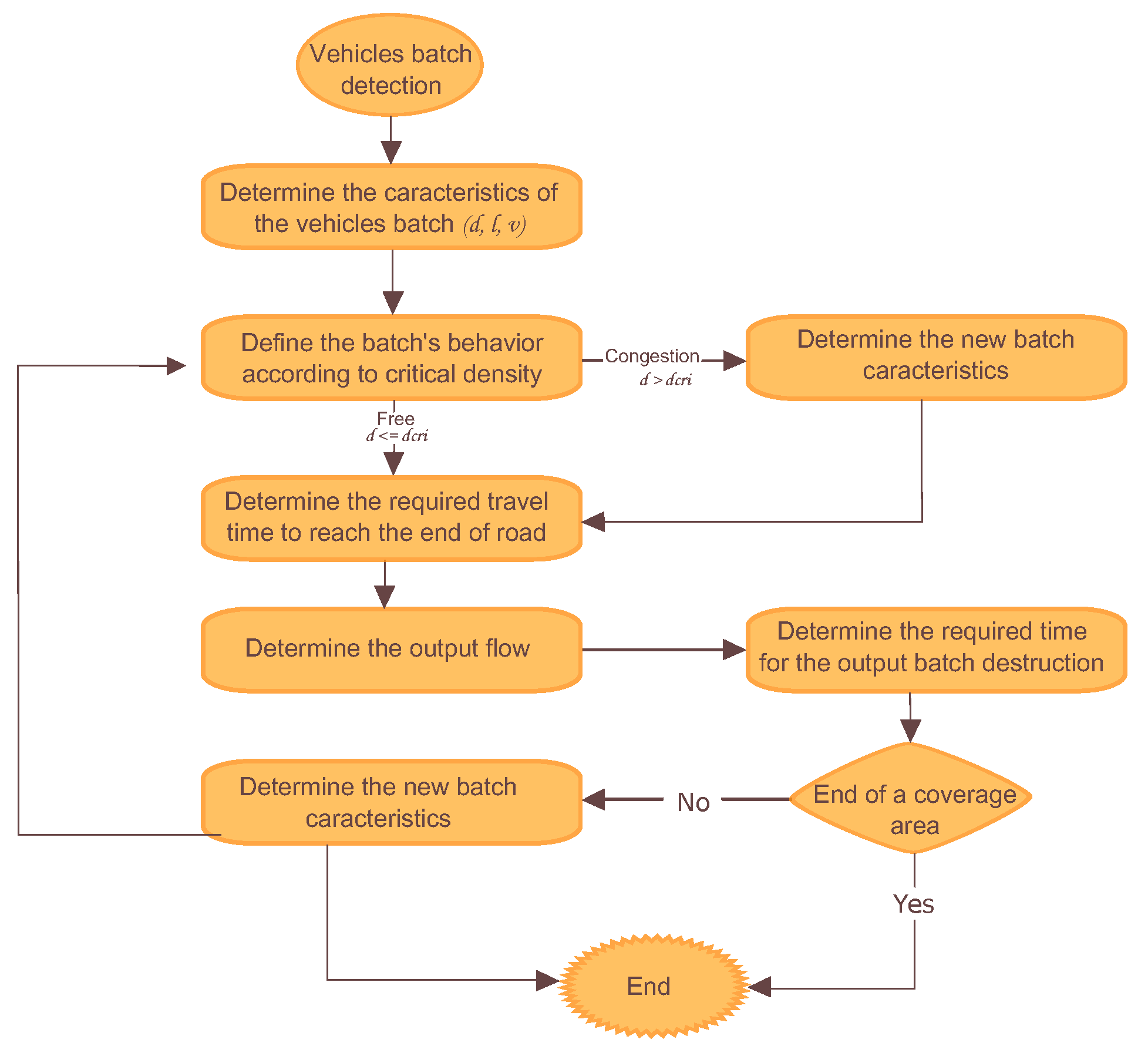
As shown in Figure 3, the Petri net model, which is implemented at the base station, starts its execution after vehicle batch detection where the main characteristics are a priori-calculated.
- Step 1:
- Determining the batch’s behavior according to the critical density.When the density of the vehicle batch is greater than the critical density of the road traveled, the controllable batch is congested. Whereas the opposite is also true; when the density of the vehicle batch is lower than the critical density of the road traveled, therefore, the controllable batch is free.
- Step 2:
- Determining the new batch’s characteristics.In the case of traffic congestion, the new characteristics of the batch have to be determined. The speed and density, in this case, vary according to the following:where is the propagation speed of congestion. In the free flow, the batch keeps performing the same behavior; therefore, its characteristics remain the same.
- Step 3:
- Determining the required travel time to reach the end of the road.To estimate the time required to traverse the road, we can divide the length of the road by the velocity of vehicle batch: .
- Step 4:
- Determining the output flow of the batch.Turning movement proportions at intersections is an essential parameter in our model since it allows estimating the output flow of the batch to different outgoing directions.According to the fundamental relation of traffic flow, the flow of a batch () is obtained as the product of the corresponding density (d) and its speed (v). .Taking into consideration the turning movement counts, we can write a dynamical equation describing the output flow of the batch as follows:where is the output flow of the batch from origin i to destination j, and are respectively the density and velocity of the batch at time t, and is the proportion of the traffic flow from origin i to destination j.
- Step 5:
- Determining the required time for the output batch destruction.To find the time, we need to divide the batch’s length by its velocity .
- Step 6:
- Determining the characteristics of the resulting batch.In case the resulting batches are within the coverage zone, we determine the new characteristics of each batch based on the output flow batch proportions, estimated in Step 4, and the characteristics of the associated road. We repeat Steps 1–6 until the coverage area is reached.
We can now carry out this procedure for the following running example.
Let there be two intersections, each composed of four single-lane road stretches, as shown in Figure 4.
At the initial state, all sections are empty, and the 114 vehicles are ready to enter the section . We consider that all vehicles are distributed uniformly among the lane. The parameters of every section are shown in the Table 1.
The traffic density is calculated by dividing the vehicle count by the corresponding road length. Therefore, the corresponding traffic density is 19 vehicles per kilometer. We resort to estimating turning movement proportions by means of predictive models (as will be discussed later) in order to determine the input flow of every stretch. For this case, let us assume that 114 vehicles are subdivided into three other separate segments in the following way:
- 46 vehicles are turning left (40%).
- 34 vehicles are traveling straight ahead (30%).
- 34 vehicles are turning right (30%).
We assume also that at the initial time, a flow of 200 vehicles enters the second road and is divided when approaching the intersection as follows:
- 120 vehicles proceeding straight ahead (60%).
- 20 vehicles turning left (10%).
- 60 vehicles turning right (30%).
The density of vehicles on the road is, therefore, 40 vehicles per kilometers.
The evolution of the traffic flow according to the model in Figure 3 is detailed below. We will illustrate both phenomena of congestion and free traffic flow introduced into GNBPN through two different scenarios. The first scenario represents the congestion regime encountered on street , while the second scenario represents the free regime encountered on the street .
Case of the free traffic flow: The vehicle batch is in free behavior and moves at its own speed along the street .
At the initial date , a batch is measured by sensor nodes at section , and there is a creation of a batch according to Definition 2. The state of the created batch is free and flows freely along the stretch since its actual density is less than the critical density (, ) as described in Section 4.3.
At , the batch reaches the end of the section and becomes an output with the following features: . As defined by Equation (6), the outputs’ flow, therefore, at the related intersection () will be split into different road segments as follows:
- .
The output controllable batch is thus . Moreover, this output batch is split into three controllable batches having the following characteristics: , , and .
At , the output batch is destroyed, which corresponds to the free behavior of the three batches. , , and .
At , the batch becomes an output batch .
At , the output batch is destroyed.
At , the output batch is destroyed.
Case of the congested traffic flow: The vehicle batch is in a congested behavior and moves with new speed and density along the street .
At , another batch is detected by sensor nodes at section , and there is the creation of a batch . The state of the created batch is congested since its density is higher than the critical density (), and therefore, the batch flows with a congested behavior along the stretch. In this example, the propagation speed of congestion is:
Thus, at , the batch becomes .
In a congestion state, a controllable batch at time t is split into two parts in contact and where: and .
The length of each vehicle’s batch can be calculated by dividing the corresponding vehicle count by the batch density.
In the example, the batch is split into the two following batches: and .
At , the batch reaches the end of the section and becomes an output controllable batch and . Moreover, at the intersection , the output controllable batch is split into three batches according to the output flow of each segment:
Therefore, the three controllable batches appear in the related road segments as follows: , , and .
At , the output batch is completely destroyed, and the becomes an output controllable batch . Therefore, three controllable batches appear in road segments and are represented as: , , and .
At , the output batch is completely destroyed. The controllable batches keep moving within the related roads with the following characteristics: , , and . Furthermore, batches and circulate according to the following characteristics: , , and .
At , the batch reaches the end of the road.
At , the batch reaches the end of the road.
At , the batch reaches the end of the road.
4.4. Turning Movement Count Models
Turning vehicle counts at intersections are needed in general for many reasons: intersection design and operation, signal timings, etc. In this article, having dynamic turning movement proportions at intersections, junctions, forks, or any kind of connected roads where the flow may be split is a required input for an accurate real-time traffic flow prediction.
In this section, we present models for estimating the traffic flow movements.
4.4.1. Random Forest
Random forest (RF) is a popular learning method that was proposed by Leon Brieman [33] for constructing a predictor ensemble with a collection of regression trees that grow in randomly-selected space data. Random forest provides two aspects that are very important: high prediction accuracy and information on variable importance for regression. In this regard, a further layer of randomness is introduced to the bagging method [34]. Additionally, RF constructs each tree based on a different bootstrap sample of the original data, and it changes how the regression trees are constructed. In a random forest, not all variables are used to choose the best split; rather, each node is split using the best among a random subset of K variables chosen at that node. While this approach seems to be more counterintuitive, it turns out to give a boost in performance compared to many existing methods and is proven to be robust against overfitting [33,35]. Besides, it is very user friendly in the sense that it needs only two parameters: the number of variables chosen randomly at each node (mtry) and the number of trees in the forest (ntree).
The algorithm of the random forests, for both classification and regression, can be presented as follows:
- Select bootstrap samples from the original dataset.
- Take each of the bootstrap samples, and grow an unpruned classification or regression trees, with the following steps: at each node, randomly select of the p predictors, and choose the best split from among those variables, rather than selecting the best split among all predictors. Bagging can be viewed as a special case of random forests if , the number of predictors.
- Each tree among the trees predicts the new data by aggregating the predictions either through averaging the values for regression or taking the majority votes for classification.
4.4.2. Neural Networks
Neural networks, originally developed for mimicking the way the basic biological neural systems work, offer several advantages over conventional methods of data analysis and modeling. Neural networks are often recognized for being adaptive; instead of being told the precise nature of a relationship or model, the data is trained to best represent the mapping relationship between the input space and output space. There are many types of neural networks. The multi-layer feed-forward neural network is one of the most commonly-used networks at the moment [36,37,38,39,40]. It is composed of many simple processing units, called neurons or nodes, that are arranged in layers. The network is constructed by joining the neurons together. The first layer of neurons sums their inputs, introduces nonlinearity by using squashing functions (e.g., using a sigmoidal function) at the hidden layers, and then, transmits a single output to all processing elements in the next layer via the connections. Data is entered in the network through the input layer and is then fed forward through one or more intermediate layers to emerge at the final layer. This is called a feed-forward network since the flow of information moves in the same direction: going from the input neurons to the output neurons. The neurons that receive information from outside the network are called the input layer. The neurons where the processed information is retrieved and used externally are called the output layer. Layers between the farmer ones are known as hidden layers; that means layers that receive information from neurons and whose output is used as a stimulus for other neurons. Through training, internal weights are determined to ensure that the neural model output best matches the desired value. In every interconnection, weights that are altered by the training step in order to generate outputs that best match the reality, and this is through a learning step aiming to adjust the weights of the connections based on the cycle from input to hidden to output pattern, e.g., backpropagation [41].
In the training procedure, we feed the network with training data or training examples to be able to learn and acquire the ability to generalize behind the examples. Then, the next step can be achieved by passing the input data by the network through the hidden layers to lead to the more suitable output.
5. Simulation
5.1. Data Preprocessing
In this study, datasets were analyzed and used as input data for simulations. The preprocessing step can improve the performance of models better than when they are fed with original data.
The following steps are performed in sequence in order to construct consistent data. Such preprocessing serves as an essential addition to yield efficient simulation results, both in terms of the capability of focusing on interesting parameters and accuracy.
5.2. Data Cleaning
We applied a data cleaning procedure to ensure consistency in the modeling results and to facilitate data analysis. This initial step is mandatory to avoid unwanted information in the studied context such as vehicle types.
5.3. Data Reorganization
When analyzing the traffic counts at any given location, the knowledge that traffic flow volumes change significantly according to each point of time is needed. They vary according to three cyclical variations that are of particular interest: hourly, daily, and monthly factors [42,43]. In this paper, we modify these factors in order to take into account other seasonal variations for estimating better the turning vehicle counts:
- Time of day: this reflects how the traffic flow changes during the day and the night;
- Day of the week: traffic varies from day to day throughout the week;
- Week of the month: indicates the traffic flow changes from week to week during the month;
- Month of the year: refers to traffic flow changes from month to month throughout the year.
In order to improve the learning step and then model accuracy, we proceeded with a reorganization step of the datasets. Consequently, in the reorganized dataset, every record represents the epoch with its related information namely minute, hour, day of the week, week of the month, month of the year, amount of vehicles turning to the left, amount of vehicles turning to the right, the amount of vehicles proceeding straight through the intersection, and the sum of the inflow into the intersection. Table 2 shows a sample of the preprocessed dataset for a given date.
5.4. Missing Data Imputation
In order to obtain a useful dataset and overcome the case of missing data, especially as the original database has has many different periods, the imputation step consists of replacing missing values with substituted values from other intersection that respect some similarity criteria. The following are the criteria of intersections’ similarity:
- Number of road segments: intersections have the same count of segments.
- Daily road traffic estimates: the estimated number of vehicles that drive through the intersection during 24 h.
- Rush hour and peak hour volume: intersections have the same period of the day during which the highest traffic volumes are observed, and they have mostly the same volumes.
6. Results
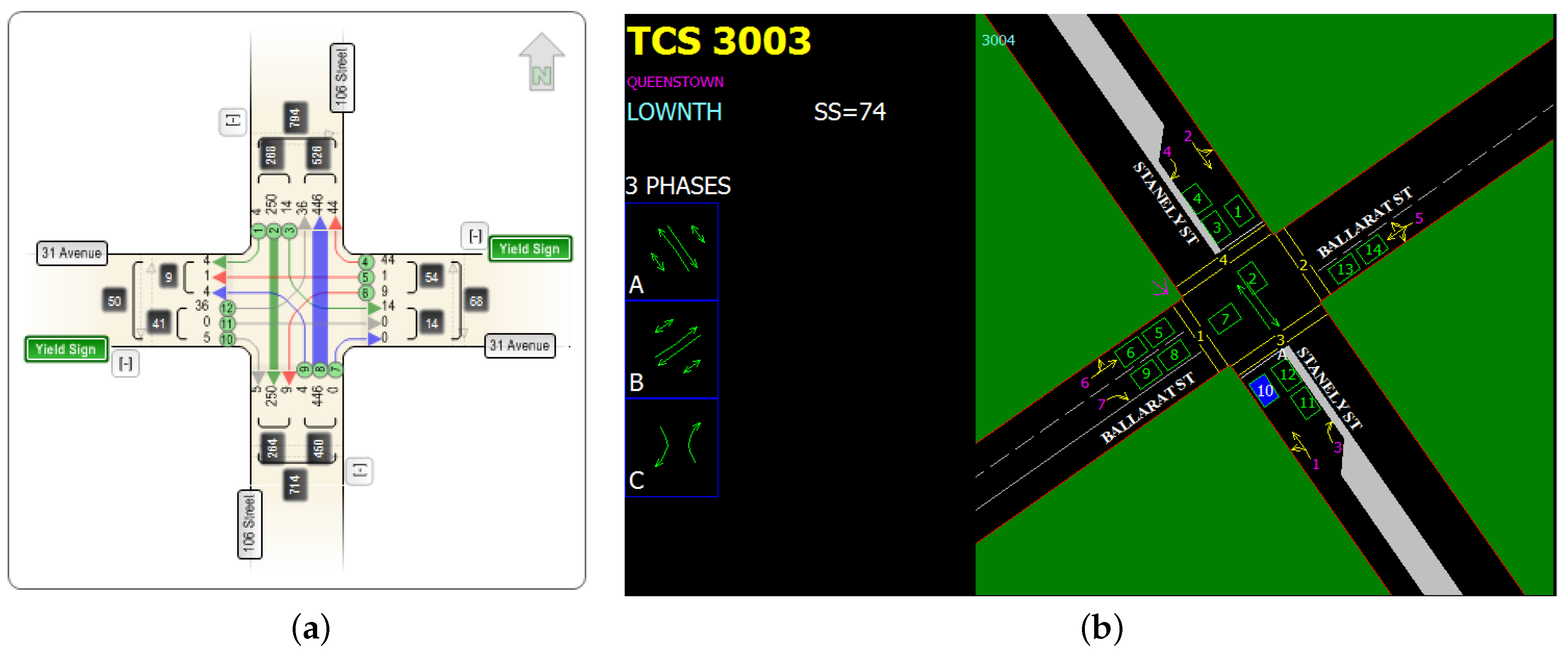
In this section, we implement the aforementioned models, and we run simulations to study the findings of each of them. The present numerical analysis is intended to conduct a comparison of models that can be utilized for estimating turning movement counts. Simulations investigated the performances of the models and were performed at two different intersections. In this regard, two different datasets were used that contained real-world collected data. The first dataset was collected from the 31 Avenue/106 Street intersection in the city of Edmonton. Canada. The data was recorded in 5-min time intervals. For the second dataset, we selected the Stanley Street/Ballarat Street intersection in New Zealand. Figure 5 shows both intersections that were used in this analysis with how the sensors were placed. We used the data of vehicles coming from Stanly St West and either turning right into Ballarat Street or continuing flowing straight into Stanly Street. The data was recorded in 15-min time intervals. As a good practice, we divided the dataset into two parts:
- The training set was used for building the model;
- The test set was used for evaluating the model and testing its predictions.
This is a valid way since it involves the training set and testing set being constructed randomly and obtains reliable estimates of the model’s performance and predictions.
Moreover, for the three machine learning techniques, the best combinations of parameter values were selected by a 10-fold cross-validation procedure, and the final models were selected based on the accuracy as the performance criterion.
Random forests: In this work, the version of the algorithm used was based on [33] and was implemented in the R package RandomForestSRC [44].
Neural network: The version of the algorithm used was based on [45] and was implemented using the R package neural net [46].
Linear regression: The version of the algorithm used was based on [47,48] and implemented in the R package random forest [48].
The accuracy of the models can be expressed using the root mean squared error (RMSE) as shown in Equation (8); we used this indicator to evaluate the quality of the predicted values of each model vs. the real observed values:
where is the real data value at time t, is the predicted data value at time t, and n is the total number of intervals.
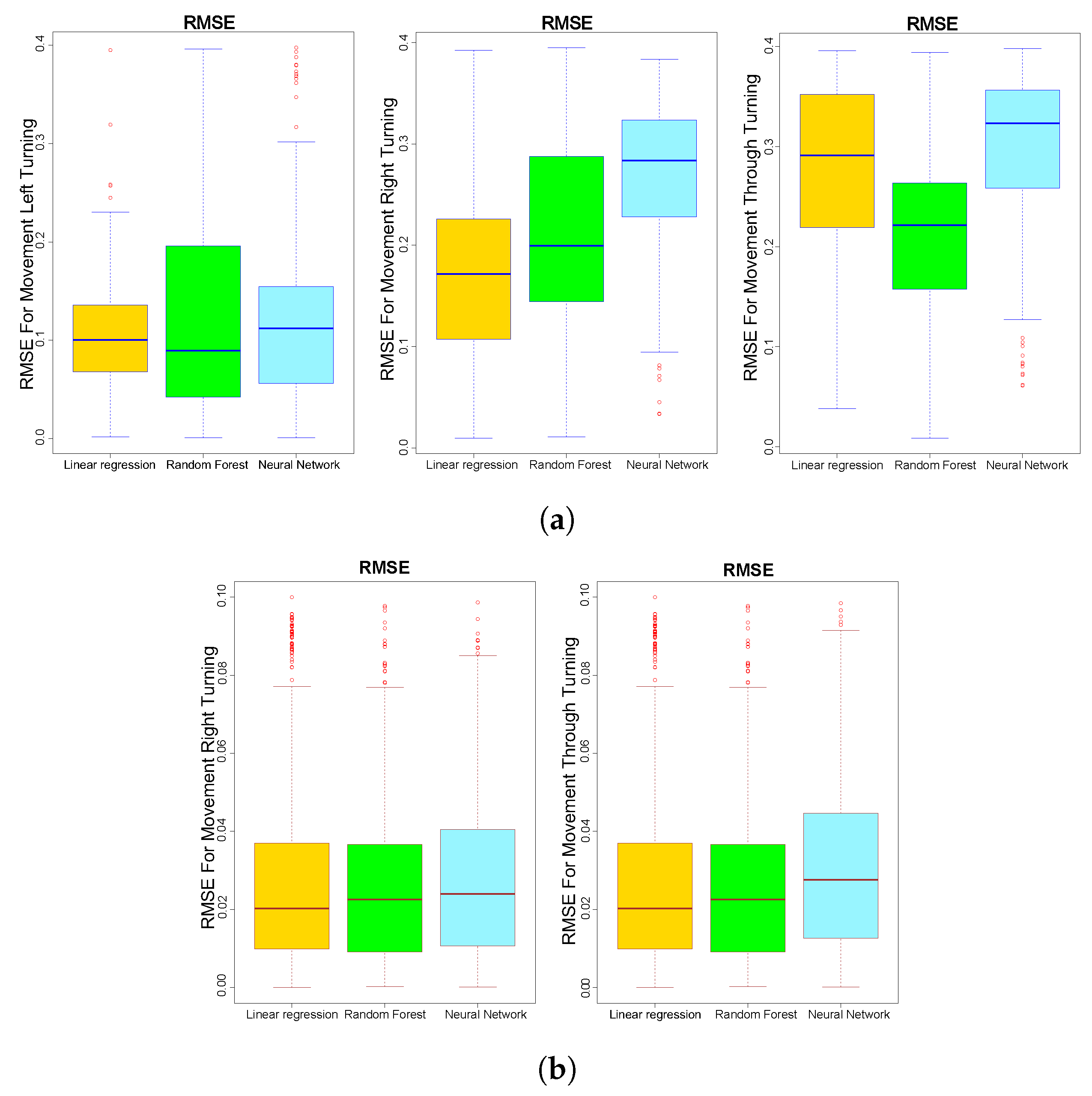
The regression results for the three models considered in this paper are illustrated using Figure 6, which presents comparative boxplots of the accuracies across both datasets we used. The horizontal solid line inside the box represents the median accuracy of the data. The bottom and top of the box represent, respectively, the first quartile and third quartile of the data. Dotes outside the box indicate outliers.
Figure 6 shows that linear regression achieved slightly higher accuracy than the other models regarding right-turning vehicles for the first dataset (median (linear regression) = ), although random forest (median = ) and the neural network (median = ) exhibited an acceptable accuracy. The same result was found for the second dataset regarding through and right-turning vehicles (median (linear regression) = 0.020, median (random forest) = 0.023, and median (neural network) = 0.024). On the other hand, Figure 6 reveals also that random forest corresponded to a high predictive performance compared to the other models for through and left-turning vehicles regarding the first dataset.
Table 3 shows that for left-turning vehicles, 35% of predictions had an accuracy between 81% and 100% for linear regression, 22.77% for random forest, and 44.44% for neural network. This shows that when there are not enough training sets, the neural network can produce better predictions compared to linear regression and random forest.
7. Conclusions
In this research, we presented the generalized nondeterministic batch Petri nets model based on the intersection turning movement for road traffic flow prediction. There were two major findings. First, all models achieved an acceptable predictive accuracy with slightly superior results for linear regression. Second, for small datasets or in the case of insufficient data amount, the neural network couold be applied to predict more reasonable results compared to other models.
We would like to complete this work in future by presenting the whole evolution of GNBPN with the different dynamics of its places’ batches at different traffic states and in more complicated scenarios, and moreover, we would like to validate the behavior of the system and its correctness by means of detailed simulations.
Author Contributions
This work is the outcome of collective efforts. Y.R. assumed the duty of conducting the study, performing simulations, and writing the manuscript with the support of L.B. and S.B., who directed the whole work in every step.
Funding
This research received no external funding.
Acknowledgments
We would like to thank the Wellington Transport Operations Centre—New Zealand for their cooperation in providing the needed dataset for our work. Furthermore, we would like to thank reviewers for their constructive remarks and suggestions to make this manuscript better and that significantly improved its quality.
Conflicts of Interest
The authors declare no conflict of interest.
Abbreviations
The following abbreviations are used in this manuscript:
| WSN | wireless sensor network |
| RF | random forest |
| WTMS | WSN-based traffic management system |
| controllable batch |
References
- Nations, U. World Cities Report 2016 Urbanization and Development: Emerging Futures; World Cities Report; United Nations Publications: New York, NY, USA, 2016. [Google Scholar]
- Centre for Economics and Business Research (Cebr); INRIX. The Future Economic and Environmental Costs of Gridlock in 2030: An Assessment of the Direct and Indirect Economic and Environmental Costs of Idling in Road Traffic Congestion to Households in the UK, France, Germany and the USA; Cebr: London, UK, 2014; p. 67. [Google Scholar]
- Rad, T.G.; Sadeghi-Niaraki, A.; Abbasi, A.; Choi, S.M. A methodological framework for assessment of ubiquitous cities using ANP and DEMATEL methods. Sustain. Cities Soc. 2018, 37, 608–618. [Google Scholar] [CrossRef]
- Randhawa, A.; Kumar, A. Exploring sustainability of smart development initiatives in India. Int. J. Sustain. Built Environ. 2017, 6, 701–710. [Google Scholar] [CrossRef]
- Pardini, K.; Rodrigues, J.J.P.C.; Kozlov, S.A.; Kumar, N.; Furtado, V. IoT-Based Solid Waste Management Solutions: A Survey. J. Sens. Actuator Netw. 2019, 8, 5. [Google Scholar] [CrossRef]
- Wieringa, J.; Kannan, P.; Ma, X.; Reutterer, T.; Risselada, H.; Skiera, B. Data analytics in a privacy-concerned world. J. Bus. Res. 2019. [Google Scholar] [CrossRef]
- Goodman, M. Future Crimes: Inside The Digital Underground and the Battle For Our Connected World; Transworld: London, UK, 2015. [Google Scholar]
- Ballard, C.; Compert, C.; Jesionowski, T.; Milman, I.; Plants, B.; Rosen, B.; Smith, H.; Redbooks, I. Information Governance Principles and Practices for a Big Data Landscape; IBM Redbooks: Armonk, NY, USA, 2014. [Google Scholar]
- Haman, I.T.; Galland, S.; Claude, J. Towards an Multilevel Agent-based Model for Traffic Simulation Towards an Multilevel Agent-based Model for Traffic Simulation. Procedia Comput. Sci. 2017, 109, 887–892. [Google Scholar] [CrossRef]
- Ngoduy, D. Commun Nonlinear Sci Numer Simulat Instability of cooperative adaptive cruise control traffic flow: A macroscopic approach. Commun. Nonlinear Sci. Numer. Simul. 2013, 18, 2838–2851. [Google Scholar] [CrossRef]
- Li, Y.; Sun, D. Microscopic car-following model for the traffic flow: The state of the art. J. Control. Theory Appl. 2012, 10, 133–143. [Google Scholar] [CrossRef]
- Li, K.; Ioannou, P. Modeling of Traffic Flow of Automated Vehicles. IEEE Trans. Intell. Transp. Syst. 2004, 5, 99–113. [Google Scholar] [CrossRef]
- Jamshidnejad, A.; Papamichail, I.; Papageorgiou, M.; Schutter, B.D. A mesoscopic integrated urban traffic flow-emission model. Transp. Res. Part C 2017, 75, 45–83. [Google Scholar] [CrossRef]
- Lighthill, M.J.; Whitham, G.B. On Kinematic Waves. II. A Theory of Traffic Flow on Long Crowded Roads. Proc. R. Soc. A Math. Phys. Eng. Sci. 1955, 229, 317–345. [Google Scholar] [CrossRef]
- Richards, P.I. Shock Waves on the Highway; Technical Operations, Inc.: Arlington, MA, USA, 1956; pp. 42–51. [Google Scholar]
- Tonguz, O.K.; Viriyasitavat, W. Modeling Urban Traffic: A Cellular Automata Approach. IEEE Commun. Mag. 2009, 47, 142–150. [Google Scholar] [CrossRef]
- Knospe, W.; Santen, L.; Schadschneider, A.; Schreckenberg, M. Towards a realistic microscopic description of highway traffic. Int. J. Mod. Phys. C 2000, 21, 1311–1327. [Google Scholar] [CrossRef]
- Pascale, A.; Nicoli, M.; Deflorio, F.; Dalla Chiara, B.; Spagnolini, U. Wireless sensor networks for traffic management and road safety. IET Intell. Transp. Syst. 2012, 6, 67. [Google Scholar] [CrossRef]
- Nagel, K.; Schreckenberg, M. A cellular automaton model for freeway traffic. J. Phys. I 1992, 2, 2221–2229. [Google Scholar] [CrossRef]
- Daganzo, C.F. The cell transmission model: A dynamic representation of highway traffic consistent with the hydrodynamic theory. Transp. Res. Part B 1994, 28, 269–287. [Google Scholar] [CrossRef]
- Daganzo, C.F. The cell transmission model, part II: Network traffic. Transp. Res. Part B Methodol. 1995, 29, 79–93. [Google Scholar] [CrossRef]
- Wang, P.; Jones, L.S.; Yang, Q. A novel conditional cell transmission model for oversaturated arterials. J. Cent. South Univ. 2012, 19, 1466–1474. [Google Scholar] [CrossRef]
- Riouali, Y.; Benhlima, L.; Bah, S. Petri net extension for traffic road modelling. Int. J. Sci. Eng. Res. 2016, 7, 7–12. [Google Scholar]
- Ghods, A.H.; Fu, L. Real-time estimation of turning movement counts at signalized intersections using signal phase information. Transp. Res. Part C 2014, 47, 128–138. [Google Scholar] [CrossRef]
- Lan, C.J.; Davis, G.A. Real-time estimation of turning movement proportions from partial counts on urban networks. Transp. Res. Part C Emerg. Technol. 1999, 7, 305–327. [Google Scholar] [CrossRef]
- Turning, I.; Models, M. Estimation of Intersection Turning Movements from Approach Counts. ITE J. 1988, 58, 41–46. [Google Scholar]
- Chen, A.; Chootinan, P.; Ryu, S.; Lee, M.; Recker, W. An intersection turning movement estimation procedure based on path flow estimator. J. Adv. Transp. 2012, 46, 161–176. [Google Scholar] [CrossRef]
- Shirazi, M.S.; Morris, B.T. Vision-Based Turning Movement Monitoring: Count, Speed & Waiting Time Estimation. IEEE Intell. Transp. Syst. Mag. 2016, 8, 23–34. [Google Scholar]
- Razouki, S.S.; Yousif, S. A new turning movement algorithm for special road junctions. SCIREA J. Agric. 2016, 1, 35–49. [Google Scholar]
- Lee, S.; Wong, S.C.; Chun, C.; Pang, C.; Choi, K. Real-Time Estimation of Lane-to-Lane Turning Flows at Isolated Signalized Junctions. IEEE Trans. Intell. Transp. Syst. 2015, 16, 1549–1558. [Google Scholar] [CrossRef]
- Jiao, P.; Liu, M.; Guo, J.; Sun, T. Bi-Bayesian Combined Model for Two-Step Prediction of Dynamic Turning Movement Proportions at Intersections. Adv. Mech. Eng. 2014, 2014, 1–9. [Google Scholar] [CrossRef]
- Gaddouri, R.; Brenner, L.; Demongodin, I. Extension of Batches Petri Nets by Bi-parts batch places. In Proceedings of the 1st International Workshop on Petri Nets for Adaptive Discrete-Event Control Systems co-located with 35th International Conference on Application and Theory of Petri Nets and Concurrency (Petri Nets 2014), Tunis, Tunisia, 24 June 2014. [Google Scholar]
- Breiman, L. Random forests. Mach. Learn. 2001, 45, 5–32. [Google Scholar] [CrossRef]
- Breiman, L. Bagging Predictors. Mach. Learn. 1996, 24, 123–140. [Google Scholar] [CrossRef]
- Liaw, A.; Wiener, M. Classification and Regression by RandomForest. Forest 2001, 23. [Google Scholar]
- Senthilkumar, M. 5 - Use of artificial neural networks (ANNs) in colour measurement. In Colour Measurement; Gulrajani, M., Ed.; Woodhead Publishing Series in Textiles; Woodhead Publishing: Sawston, UK, 2010; pp. 125–146. [Google Scholar]
- Tutak, M.; Brodny, J. Predicting Methane Concentration in Longwall Regions Using Artificial Neural Networks. Int. J. Environ. Res. Public Health 2019, 16, 1406. [Google Scholar] [CrossRef]
- Abdi-Khanghah, M.; Bemani, A.; Naserzadeh, Z.; Zhang, Z. Prediction of solubility of N-alkanes in supercritical CO2 using RBF-ANN and MLP-ANN. J. CO2 Util. 2018, 25, 108–119. [Google Scholar] [CrossRef]
- Ebrahimpour, R.; Nikoo, H.; Masoudnia, S.; Yousefi, M.R.; Ghaemi, M.S. Mixture of MLP-experts for trend forecasting of time series: A case study of the Tehran stock exchange. Int. J. Forecast. 2011, 27, 804–816. [Google Scholar] [CrossRef]
- Gardner, M.W.; Dorling, S.R. Artificial neural networks (the multilayer perceptron)—A review of applications in the atmospheric sciences. Atmos. Environ. 1998, 32, 2627–2636. [Google Scholar] [CrossRef]
- Rumelhart, D.E.; Hinton, G.E.; Williams, R.J. Neurocomputing: Foundations of Research; Chapter Learning R; MIT Press: Cambridge, MA, USA, 1988; pp. 696–699. [Google Scholar]
- Institute of Transportation Engineers; Wolshon, B.; Pande, A. Traffic Engineering Handbook; Wiley: Hoboken, NJ, USA, 2016. [Google Scholar]
- Sivakumar, B.; Ghosn, M.; Moses, F. Protocols for Collecting and Using Traffic Data in Bridge Design; NCHRP Report; Transportation Research Board: Washington, DC, USA, 2011. [Google Scholar]
- Ishwaran, H.; Kogalur, U. randomForestSRC: Random Forests for Survival, Regression and Classification (RF-SRC). 2016. Available online: https://kogalur.github.io/randomForestSRC/theory.html (accessed on 26 August 2019).
- Matausek, M.R.; Miljkovic, D.M.; Jeftenic, B.I. Nonlinear multi-input-multi-output neural network control of DC motor drive with field weakening. IEEE Trans. Ind. Electron. 1998, 45, 185–187. [Google Scholar] [CrossRef]
- Günther, F.; Fritsch, S. Neuralnet: Training of Neural Networks. R J. 2010, 2, 30. [Google Scholar] [CrossRef]
- Kaya Uyanık, G.; Güler, N. A Study on Multiple Linear Regression Analysis. Procedia Soc. Behav. Sci. 2013, 106, 234–240. [Google Scholar] [CrossRef] [Green Version]
- Egoshin, V.; Ivanov, S.; Savvina, N.; Ermolaev, A.; Mamyrbekova, S.; Zhamaliyeva, L.; Grjibovski, A. Correlation and simple regression analysis using R. Hum. Ecol. 2018, 2018, 55–64. [Google Scholar] [CrossRef]
Figure 1.
T-intersection with the stop rule.

Figure 2.
The system flow chart.

Figure 3.
The procedure of the model execution.

Figure 4.
Example of two intersections that can be running the generalized nondeterministic batch Petri net (GNBPN) model.
Figure 4.
Example of two intersections that can be running the generalized nondeterministic batch Petri net (GNBPN) model.

Figure 5.
Illustration of intersections that are used in the simulations. (a) The 31 Avenue/106 Street intersection in the city of Edmonton, Canada; (b) The Stanley Street/Ballarat Street intersection in New Zealand.
Figure 5.
Illustration of intersections that are used in the simulations. (a) The 31 Avenue/106 Street intersection in the city of Edmonton, Canada; (b) The Stanley Street/Ballarat Street intersection in New Zealand.

Figure 6.
Turning estimation for through, left, and right movements. (a) Turning movement counts for the 31 Avenue/106 Street intersection. (b) Turning movement counts for the Stanley Street/Ballarat Street intersection.
Figure 6.
Turning estimation for through, left, and right movements. (a) Turning movement counts for the 31 Avenue/106 Street intersection. (b) Turning movement counts for the Stanley Street/Ballarat Street intersection.


Table 1.
Parameters of both sections et .
| Section | ||
|---|---|---|
| (km) | 6 | 5 |
| () | 40 | 80 |
| () | 200 | 100 |
| () | 2000 | 2000 |
Table 2.
A sample of data after the pre-processing step.
| Day of Week | Week of Month | Month of Year | ms | ss | pmam | L | T | R | Sum |
|---|---|---|---|---|---|---|---|---|---|
| 4 | 2 | 3 | 7 | 25 | 1 | 2 | 55 | 77 | 134 |
Table 3.
The prediction accuracy for left-turning vehicles.
| Percentage Accuracy | Linear Regression | Random Forest | Neural Network |
|---|---|---|---|
| 81%–100% | 35 | 22.7 | 44.4 |
© 2019 by the authors. Licensee MDPI, Basel, Switzerland. This article is an open access article distributed under the terms and conditions of the Creative Commons Attribution (CC BY) license (http://creativecommons.org/licenses/by/4.0/).
Share and Cite
MDPI and ACS Style
Riouali, Y.; Benhlima, L.; Bah, S. An Integrated Turning Movements Estimation to Petri Net Based Road Traffic Modeling. J. Sens. Actuator Netw. 2019, 8, 49. https://doi.org/10.3390/jsan8030049
AMA Style
Riouali Y, Benhlima L, Bah S. An Integrated Turning Movements Estimation to Petri Net Based Road Traffic Modeling. Journal of Sensor and Actuator Networks. 2019; 8(3):49. https://doi.org/10.3390/jsan8030049
Chicago/Turabian StyleRiouali, Youness, Laila Benhlima, and Slimane Bah. 2019. "An Integrated Turning Movements Estimation to Petri Net Based Road Traffic Modeling" Journal of Sensor and Actuator Networks 8, no. 3: 49. https://doi.org/10.3390/jsan8030049
Note that from the first issue of 2016, this journal uses article numbers instead of page numbers. See further details here.