


Underwater Wireless Sensor Network Performance Analysis Using Diverse Routing Protocols
by
 , and
, and
Kaveripaka Sathish
1,
Chinthaginjala Venkata Ravikumar
1,*,
Anbazhagan Rajesh
2 and
Giovanni Pau
3,*
1
School of Electronics Engineering, Vellore Institute of Technology, Vellore 632014, India
2
School of Electrical and Electronics Engineering, SASTRA University, Thanjavur 613401, India
3
Faculty of Engineering and Architecture, Kore University of Enna, 94100 Enna, Italy
*
Authors to whom correspondence should be addressed.
J. Sens. Actuator Netw. 2022, 11(4), 64; https://doi.org/10.3390/jsan11040064
Submission received: 16 September 2022
/
Revised: 29 September 2022
/
Accepted: 4 October 2022
/
Published: 9 October 2022
(This article belongs to the Special Issue Optimization within Sensor Networks and Telecommunications)
Abstract
:The planet is the most water-rich place because the oceans cover more than 75% of its land area. Because of the unique activities that occur in the depths, we know very little about oceans. Underwater wireless sensors are tools that can continuously transmit data to one of the source sensors while monitoring and recording their surroundings’ physical and environmental parameters. An Underwater Wireless Sensor Network (UWSN) is the name given to the network created by collecting these underwater wireless sensors. This particular technology has a random path loss model due to the time-varying nature of channel parameters. Data transmission between underwater wireless sensor nodes requires a careful selection of routing protocols. By changing the number of nodes in the model and the maximum speed of each node, performance parameters, such as average transmission delay, average jitter, percentage of utilization, and power used in transmit and receive modes, are explored. This paper focuses on UWSN performance analysis, comparing various routing protocols. A network path using the source-tree adaptive routing-least overhead routing approach (STAR-LORA) Protocol exhibits 85.3% lower jitter than conventional routing protocols. Interestingly, the fisheye routing protocol achieves a 91.4% higher utilization percentage than its counterparts. The results obtained using the QualNet 7.1 simulator suggest the suitability of routing protocols in UWSN.
1. Introduction
Although water covers a large portion of our planet, much of it is still unknown [1,2,3,4]. Exploration in this region has significantly increased recently. In addition to being endowed with abundant natural resources, it has contributed significantly to developing ships, oil pipelines, and the military. This situation represents the researcher’s top priority in environments such as oceans, seas, and the like, which contain enormous amounts of naturally occurring data. By developing various UWSN protocols for the underwater environment, the developers have gathered and analyzed a significant amount of data to some extent [5,6,7,8]. Research in this area is built on the findings of earlier studies, as described in the background information below. The general structure of underwater wireless communication is depicted in Figure 1. Routing protocols are used to transfer routing information from one routing device to another. Because network circumstances change over time, this information is crucial for ensuring that packets arrive at their destinations.
1.1. Proactive Routing Protocols
When it comes to routing protocols of this sort, the path that will be taken between nodes is determined in advance. The most recent route between different nodes in the network needs to be meticulously maintained at all times. On the other hand, for particularly dynamic network topologies, proactive schemes place an emphasis on the management of significant amounts of resources in order to maintain the accuracy and consistency of routing information. In such designs, the finding overheads are significant because one needs to discover all of the nodes. Therefore, there will be no delay in transmission if a route has already been obtained by a node before the traffic arrives at that node. Nodes will periodically share their information with one another in proactive routing protocols as a reaction to topological changes that have been caused. The primary benefit is that it reduces the amount of time that is wasted waiting on a needed route when there is initiating traffic to a required destination and it determines in a short amount of time whether or not a destination is attainable. It is possible that a substantial number of network resources will be used up during the procedure.
1.2. Reactive Routing Protocols
In this type of routing protocol, the path between the nodes is formed when a node decides it wants to exchange its packets. As it moves from the source node to the destination node, this node now starts the process of route discovery in advance. The method is considered successful when a route is recognized by both nodes in the hypothetical situation. This type of data transfer is recorded in a table along with each potential path, starting at the source and remaining there until the route is no longer required. Each intermediate node is essential for maintaining the link’s records between the source and the destination. These intermediary nodes will help send the replies back to the source after a request has been issued to the destination from the source node. Data traffic will start being transmitted to the destination as soon as the source node receives the response.
1.3. Hybrid Protocols
The proactive and reactive routing techniques have been combined to create the hybrid routing protocol. It is believed that the protocols at issue combine elements from both of the aforementioned groups. It is envisaged that the utilization of this scenario will allow for a reduction in the overheads associated with route discovery, as well as the realization of the benefits of both proactive and reactive routing methods.
1.4. Ad Hoc On-Demand Distance Vector Routing (AODV) Protocol
A reactive traffic routing protocol to support AODV, existing paths merely need to have their routing changed [9]. Information about routing is kept in the routing tables of nodes. Each mobile node has its own “next-hop routing database,” which stores details about the nodes it can connect to in the next hop. If a routing table entry is inactive for a certain amount of time without being utilized or activated again, it may be destroyed. The AODV uses the same on-demand utilization of the destination sequence number method as the DSDV. When there is no known route to the destination, AODV will start the route discovery process using the transmitting node. The source will broadcast route request (RREQ) packets to the network in an effort to hasten the process of routing discovery. The addresses of the transmitting and receiving nodes, the broadcast ID used to identify the packet, the sequence number last seen at the destination node, and the sequence number last seen at the sending node are all information that is provided by RREQs. In order to create routes that are both current and error-free, sequence numbers are a need. A node may use the expanding ring search strategy to ignore previously received RREQs and so reduce the amount of flooding overhead during the route-finding process. The RREQs Time-To-Live will be significantly compressed in its early stages (TTL). In the case that more RREQ attempts to the same destination fail, the TTL will be prolonged.
1.5. Dynamic Source Routing (DSR) Protocol
The dynamic source routing protocol (DSR) is one kind of on-demand routing system. DSR is a simple yet powerful routing algorithm designed specifically for use in multi-hop wireless ad hoc networks with mobile nodes. Using DSR, the network is able to completely self-organize and self-configure, eliminating the requirement for a centralized network administration structure. Two major techniques work together to make the DSR protocol possible for ad hoc networks to discover and keep track of their source routes. The DSR protocol incorporates these elements.
The Path’s Uncovering: In order to transfer a packet from node S to node D, node S must first locate a source route to node D. The method used is called “route discovery.” Path discovery is used only when S wants to send a packet to D but does not know a route to D.
The phrase “route maintenance” refers to the technique that allows a node S, while utilizing a source route to D, to ascertain whether or not the topology of the network has changed in such a way that it is no longer possible for it to use its route to D due to a link along the route being inoperable. The mechanism for this is the upkeep of the routes. Because one of the source routes was discovered to be broken during routine maintenance. S can either try sending the packet over a different path it knows leads to destination D, or it can re-initiate route discovery to find a new path. If S is not actively sending packets to D, then this route will not be maintained.
1.6. Zone Routing Protocol (ZRP)
The zone routing protocol (ZRP) [10] is a reactive protocol for zone communication and proactive discovery inside a node’s immediate neighborhood. These two aspects of the protocol will be described further below. This combination technique combines the greatest characteristics of reactive and proactive methods into a single, easy-to-implement strategy. It is logical to suppose that in a MANET, the majority of interactions occur between nodes that are physically close to one another. The zero trust protocol (ZRP) is not a stand-alone protocol but rather a framework that helps other protocols run smoothly. This decoupling of a node’s local surroundings from the network’s global design enables the employment of a diverse collection of approaches, each of which has its own set of advantages when used appropriately. This is possible because a node’s neighborhood is independent of the network’s global topology. These smaller, more manageable communities are referred to as “zones,” and each node may reside within numerous overlapping zones of varying sizes. Instead of utilizing geographical coordinates, a radius of length is utilized to calculate a zone’s “size,” signifying the number of hops from the zone’s perimeter. This distance is used to compute the so-called “size” of a zone. The zone routing protocol divides the system into overlapping, varying-sized zones. A ZRP is not a single component but rather a set of parts that, when combined, provide a sophisticated routing system. This will only be feasible if every component is used. Each component runs autonomously and may apply a wide range of technologies to achieve optimal performance in the specialized areas in which it specializes. The ZRP can be disassembled into its constituent parts, which are the IARP, IERP, and BRP.
1.7. Location Aided Routing (LAR)
The LAR protocol is utilized as a form of location-based and reactive routing in wireless ad hoc networks. It does this by making use of three distinct packets, namely, the route request, the route reply, and the route error, in order to send and receive information between nodes and maintain stable connections. LAR is an on-demand routing protocol that operates in a manner analogous to that of DSR (dynamic source routing). In contrast to DSR, the LAR protocol makes use of location data in order to define the boundaries of the “request zone,” which is the area in which it is possible to discover new routes. As a direct consequence of this, the route requests will be sent only by the nodes that are part of the request zone, as opposed to being broadcast to the entirety of the network. The originator, using data from the past, makes a prediction about a spherical region called the predicted zone, which is the location in which the target object is most likely to be found at this same moment. The traveler’s average speed, in addition to the time and date associated with the traveler’s previous locations, is used to calculate not only the location of the pinpoint but also the size of its surrounding area. Find the smallest rectangle that encompasses both the targeted zone and the source in order to identify the request zone. There have been many different attempts made to raise performance standards by altering the dimensions and layout of the request zone.
A packet that contains the four corner coordinates is transmitted whenever a route discovery method is started up. Only those in this particular region will be able to listen to RREQ broadcasts. As a result, the node that is part of the request zone will proceed with the normal forwarding of the packet after it has received RREQ. However, if a node that is not within the request zone receives an RREQ, the group will be discarded by that node immediately.
1.8. Optimized Link State Routing (OLSR)
OLSR, which stands for “optimized link state routing,” is a dynamic routing technology that is frequently employed. Transmissions of routing information at regular intervals from each node in the network ensure that all of the nodes in the network share the same comprehensive view. The protocol’s periodic nature results in a large amount of additional overhead being incurred. This problem is solved by OLSR, which reduces the amount of traffic that may be forwarded. In order to accomplish this, multi-point relays, also known as MPRs, are utilized; these devices are in charge of relaying and routing messages. Each node selects MPRs manually from among the nodes that are immediately adjacent to it. It is preferable for a node to choose MPRs that will enable it to communicate with at least one of its neighbors that is accessible over a hop-and-a-half path. It is the job of the MPRs to transmit the control traffic that is produced by those nodes.
1.9. Source Tree Adaptive Routing (STAR)
In a network context, such as the internet or an ad hoc network, the STAR protocol is intended to be utilized by mobile as well as stationary nodes. This is because the protocol was designed to be universally applicable. The parameters of the source routing tree are necessary for the neighboring routers of a STAR router. The source routing tree contains every connection that the router needs to have in order to communicate with any host or combination of hosts that are located on the internet or in the ad hoc network. After gaining knowledge of new destinations, the likelihood of loops, the chance of node failure, or the splitting of a network, a router will only update the source routing tree that it uses to route traffic. Because of this, the router’s data transfer capability and power consumption will both be reduced.
The STAR routing protocol can be implemented in a variety of distinct ways, such as with an ORA or a least-overhead routing strategy, to name just a couple of the available options. This is sometimes abbreviated to ORA, which stands for “optimal routing approach” (LORA). The first strategy takes into account several statistics in order to determine which links between nodes will be the most beneficial. The effectiveness of this method does not depend on the total quantity of messages to be routed; rather, it is determined by how frequently the routing table is refreshed. The LORA technique, on the other hand, stays true to its name by putting an emphasis on the achievement of instantaneous message transmission at the price of optimality in accordance with the ORA requirements. This analysis concentrates on STAR-LORA since it offers a more direct comparison with on-demand routing protocols and is more interesting algorithmically. Additionally, this comparison can be made more easily.
1.10. Dynamic MANET on Demand Routing Protocol (DYMO)
DYMO is an innovative reactive (on-demand) routing protocol that is currently being developed in a simpler design. This helps to minimize the system requirements of participating nodes and makes it easier to implement the protocol. DYMO maintains the tried-and-true techniques of previously investigated routing protocols, such as the use of sequence numbers to ensure the absence of loops. At the same time, DYMO expands the purview of the MANET working group that is part of the Internet Engineering Task Force (IETF). DYMO makes use of the knowledge gained from prior methods of reactive routing, most notably the routing protocol AODV. It intends to provide path accumulation and cover all potential scenarios involving a gateway between a MANET and the internet as part of its features.
1.11. Fisheye State Routing (FSR)
Fisheye state routing, often known as FSR, is a routing technology for ad hoc networks that is multilayer and table-driven. It employs the scope technique. The goal is to reduce the amount of overhead that is associated with routing in extremely large, rapidly changing, and dynamic networks. According to its scope technique, the connection state changes are periodically broadcast at a defined frequency. The entirety of the network is divided into a variety of scopes, each of which is determined by the number of hops that are required to reach a specific node. The nodes that are deemed to be within this distance of one another are known as inner nodes, while the nodes that are further out are known as outer nodes. At a variety of different frequencies, neighbors obtain transmissions of the latest connection state updates. When communicating with more immediate neighbors, the information is transmitted at a lower frequency while simultaneously increasing its frequency. As a direct consequence of this, the nodes obtain connection state updates that are more accurate. It enhances the accuracy of the path over which packets are transmitted. As a consequence of this, FSR makes significant reductions in the connection overhead caused by the updating of routing tables. The ability of large mobile ad hoc networks to scale is improved as a result of this. It is suitable for rapidly changing topologies since it does not send any control signals when a link is severed. This makes it very flexible. The distance scope of the future fisheye state message exchange will not include the links that could not be established. In a mobile network that is dynamic, the links are kept fresh and free of loops by the use of regular table updates and sequence numbers [11].
Ad-hoc wireless networks, known as wireless sensor networks (WSNs), provide a wireless communication setup, such as underwater wireless communication [12]. Routing protocols for ad-hoc networks include AODV, DSR, DYMO, LAR1, Bellman-Ford, OLSR, Fisheye, STAR-ORA, ZRP, and STAR-LORA, among others [13]. The mobility model shows the movement of nodes and how their positions, speeds, and accelerations alter over time. When researching a new network protocol, it is crucial to simulate and assess its performance. The mobility model and the communicating traffic pattern are crucial in protocol simulation. Mobility models are used to describe user movement patterns. The traffic model describes the state of mobile services [14,15,16,17,18]. Figure 2 illustrates a realistic 3D underwater wireless communication scenario with various nodes. The potential challenges posed by the surrounding subsurface environment must be given the attention and consideration they require when considering underwater sensor networks [19,20,21]. The host conditions present numerous difficulties, including three-dimensional topology and continuous node movement. Additionally, many underwater applications, such as those used for detection or rescue missions, tend to be ad-hoc [22,23,24,25,26,27].
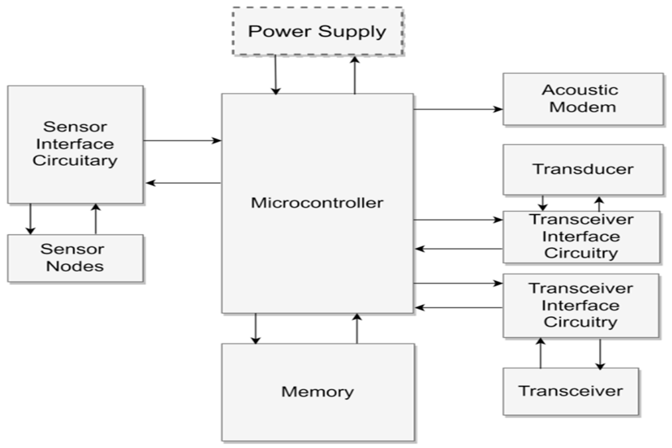
As depicted in Figure 3, a WSN comprises spatially dispersed autonomous (self-organized) sensors that monitor environmental or physical conditions, such as temperature, sound, vibration, pressure, motion, or pollutants, and cooperatively transmit their data through the network to a central location. Modern networks are bi-directional, allowing for the control of sensor activity as well. Military usage of wireless sensor networks, such as battlefield surveillance, served as the impetus for their development. Today, these networks are employed in various commercial and consumer applications, including machine health monitoring, process control, and industrial process monitoring [28]. The WSN is composed of “nodes” ranging in number from a few to thousands and are each connected to one or more sensors. Figure 3 depicts the main parts of a sensor node, which include the following subsystems: a communication (transceiver) subsystem, a computing (processing) subsystem, a sensor subsystem, and a unified power supply system.
The main contribution of the manuscript is highlighted as follows:
- Implementation of a source tree adaptive routing least overhead routing approach (STAR-LORA) protocol and a fisheye routing protocol for UWSN;
- Comparison of the STAR-LORA and fisheye routing protocols with standard routing protocols in the literature, namely, AODV, DSR, DYMO, LAR1, Bellman-Ford, OLSR, Fisheye, STAR-ORA, and ZRP;
- Analysis of the energy efficiency of the routing protocol with an increasing number of underwater wireless sensor nodes;
- Examination of the trade-off between average transmission delay, average jitter, utilization rate, and energy in transmitting and receiving modes;
- Recommendation of an appropriate routing protocol for UWSN based on the targeted performance metric.
2. Related Works
This section of the article examines previous work from the standpoint of network architecture, as well as the multiple performance measures that support the concept of extending network life.
Bhattacharjya et al. investigated a universal wireless sensor network (UWSN) using a grid topology. This study investigates energy usage across a variety of energy modalities as well as network performance.
Yildiz et al. Investigate optimizing packet size in order to maximize the longevity of UWSNs. This is done to determine how to obtain the most out of UWSNs. To maximize the longevity of a network, it is critical to consider not only the length of time it takes for a packet to transmit but also its total size. Furthermore, we mimic the connection layer in a realistic manner to reduce the amount of power consumed by the network.
Here, an optimal, collaborative, and resource-saving strategy is being examined [29]. In order to create a UWSN that consumes less energy, a relay node is chosen. The indices of dead and end-to-end delays, dead packet delivery ratio, and energy usage are investigated. The nodes are organized in a two-dimensional environment with a regular distribution. In the case of UWSN, both interference and noise are considered. Khan et al. examine interference-free localization routing for ultra-wideband sensor networks (UWSNs), with the goal of minimizing the energy hole [30]. It specifies the total number of dropped packets, the total number of dead nodes, a packet received at the sink, the total amount of energy used, and the total number of dropped packets.
A MAC protocol study was carried out at the UWSN (Park and Rodoplu 2007). It was also determined that the protocol’s scalability, energy efficiency, distributed nature, and capacity to function regardless of propagation latency or UWSN medium length. The simulation contains no propagation delay as well as a significant amount of propagation delay. In the event of a collision, the transmitted energy waste is analyzed in relation to the number of nodes and the duty cycle.
UWSN performance parameters include packet delivery ratio, network lifetime, energy utilization, and transmission latency. In terms of mobility, Alkindi et al. investigate a grid-based routing technique for UWSN [31]. Energy usage, network density, packet delivery ratio, and latency are all discussed. EAVARP, a void-avoidant and energy-conscious routing system, is being investigated by Wang et al. for wireless sensor networks [32]. UWSN is impervious to transmission, vacancy, and flooding cycles.
3. Network Scenario
The QualNet program is a simulator that can emulate the behavior of a network. A network can be established in an atmosphere free of risk and expense by employing the use of a simulation. The network design tool that comes with the QualNet 7.1 simulator provides users with an intuitive interface for the purpose of configuring simulation settings and generating network scenarios. Building a network architecture using a drag-and-drop interface is now a simple and rapid process. Reviewing the statistical data that was created by the QualNet network simulator is accomplished through the usage of its Analyzer graphic user interface. A statistics file with the extension. The stat is generated whenever a simulator is started from inside of Architect. The findings of the simulation are presented in this document. Because it is stored in text format, the basic statistics file can be accessed by using any text editor that supports text. Graphs such as this one could be constructed with the use of statistical data [33,34].
- ➢
- The scenario planning phase involves building a model of the network via a random waypoint model;
- ➢
- In the second stage, data is collected from the source node to the destination node using various traffic load applications, such as CBR, VBR, and FTP;
- ➢
- The third step is to put in place routing protocols and run simulations of potential network configurations;
- ➢
- In the fourth place, we have a comparison of the results of various assessments of the performance of ad hoc routing systems;
- ➢
- Analysis and interpretation of results constitute the final step.
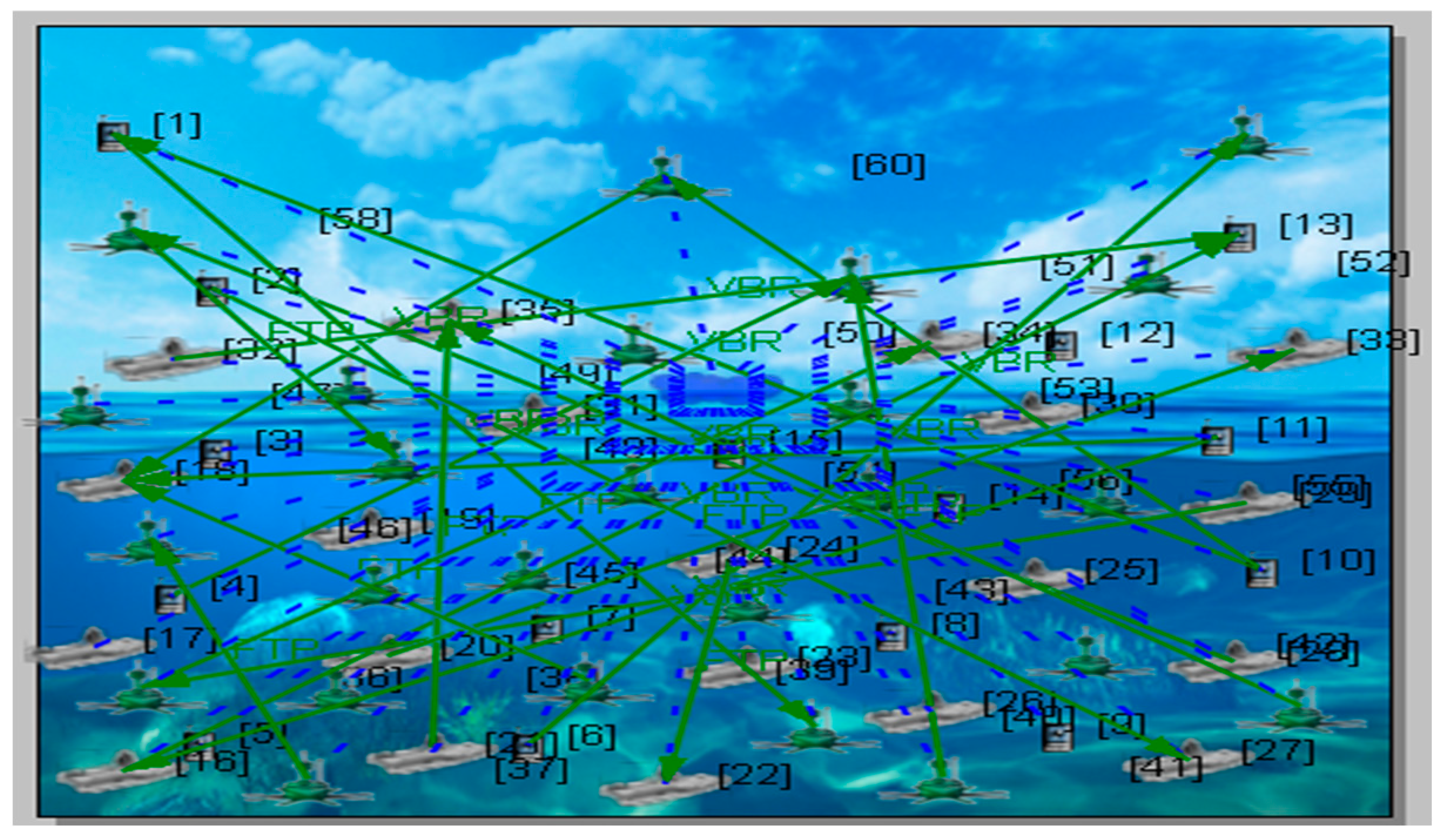
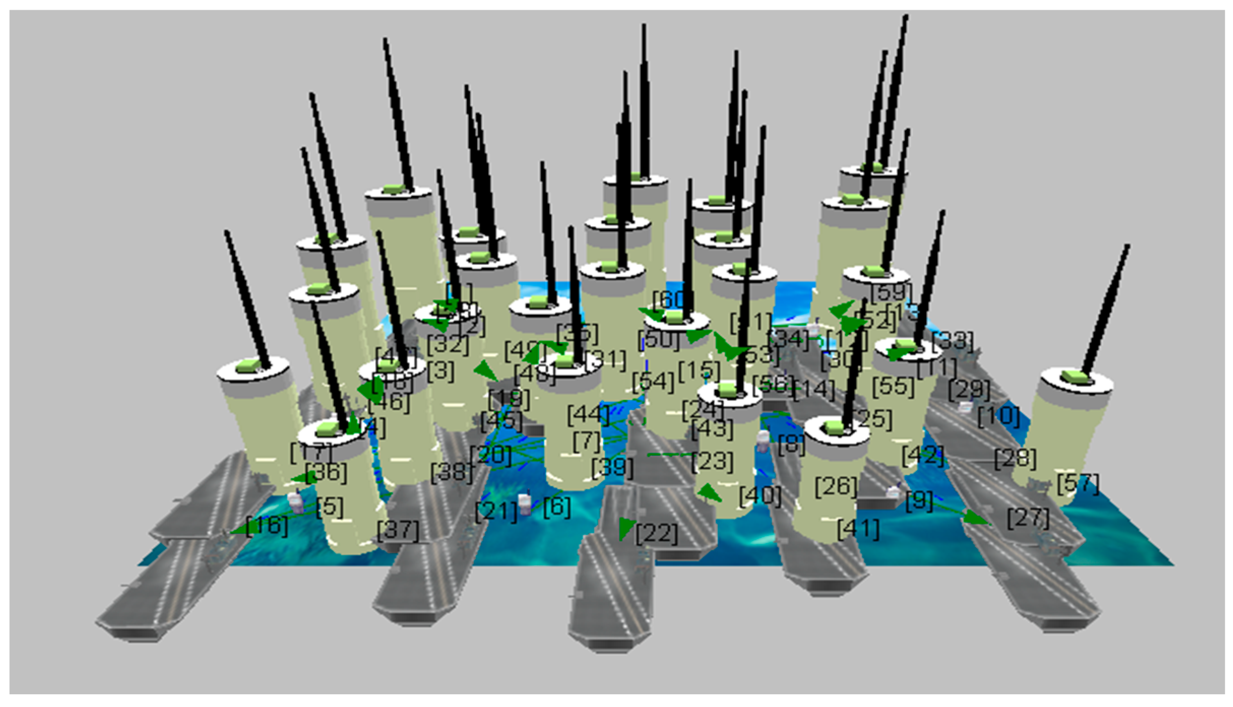
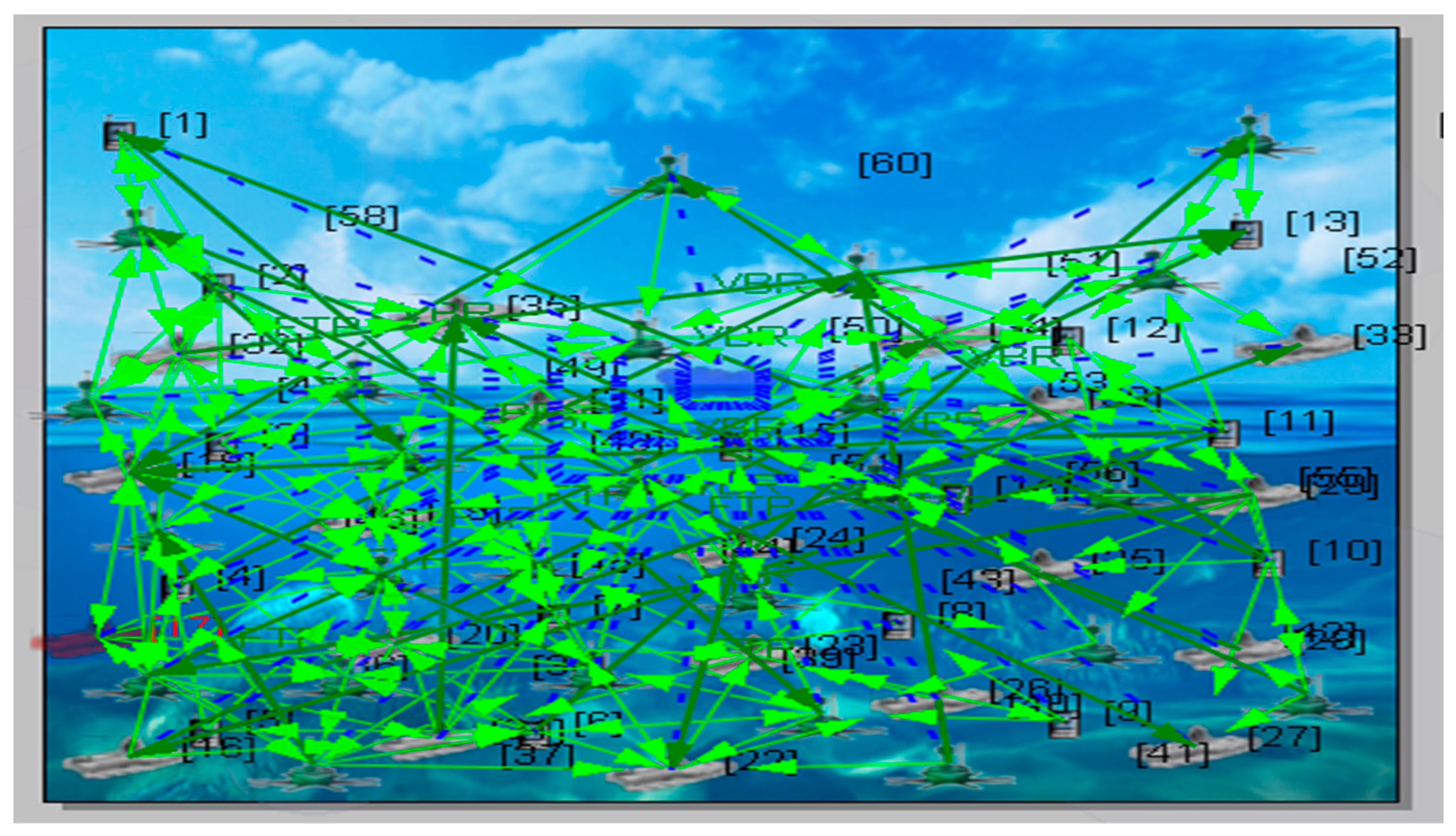
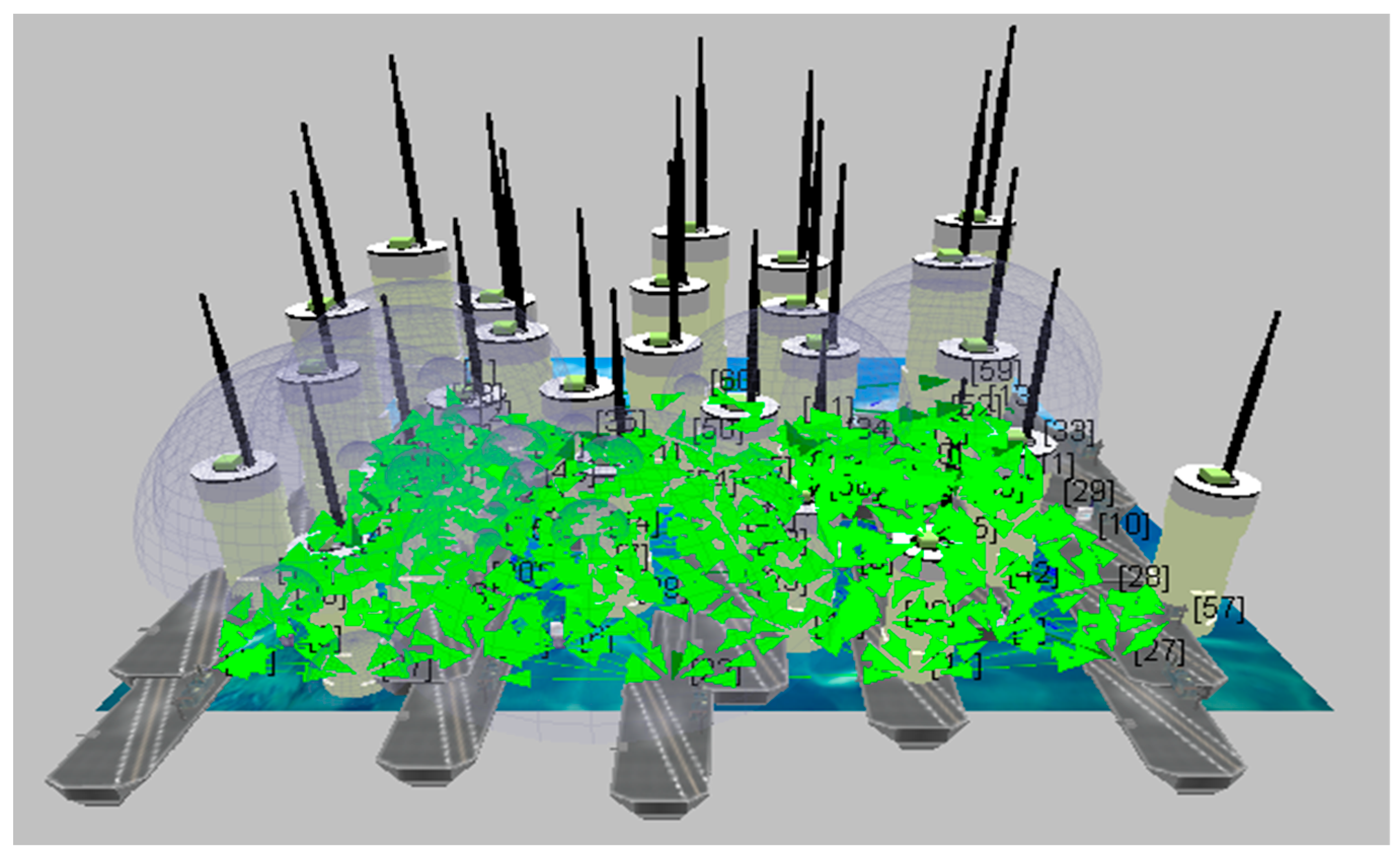
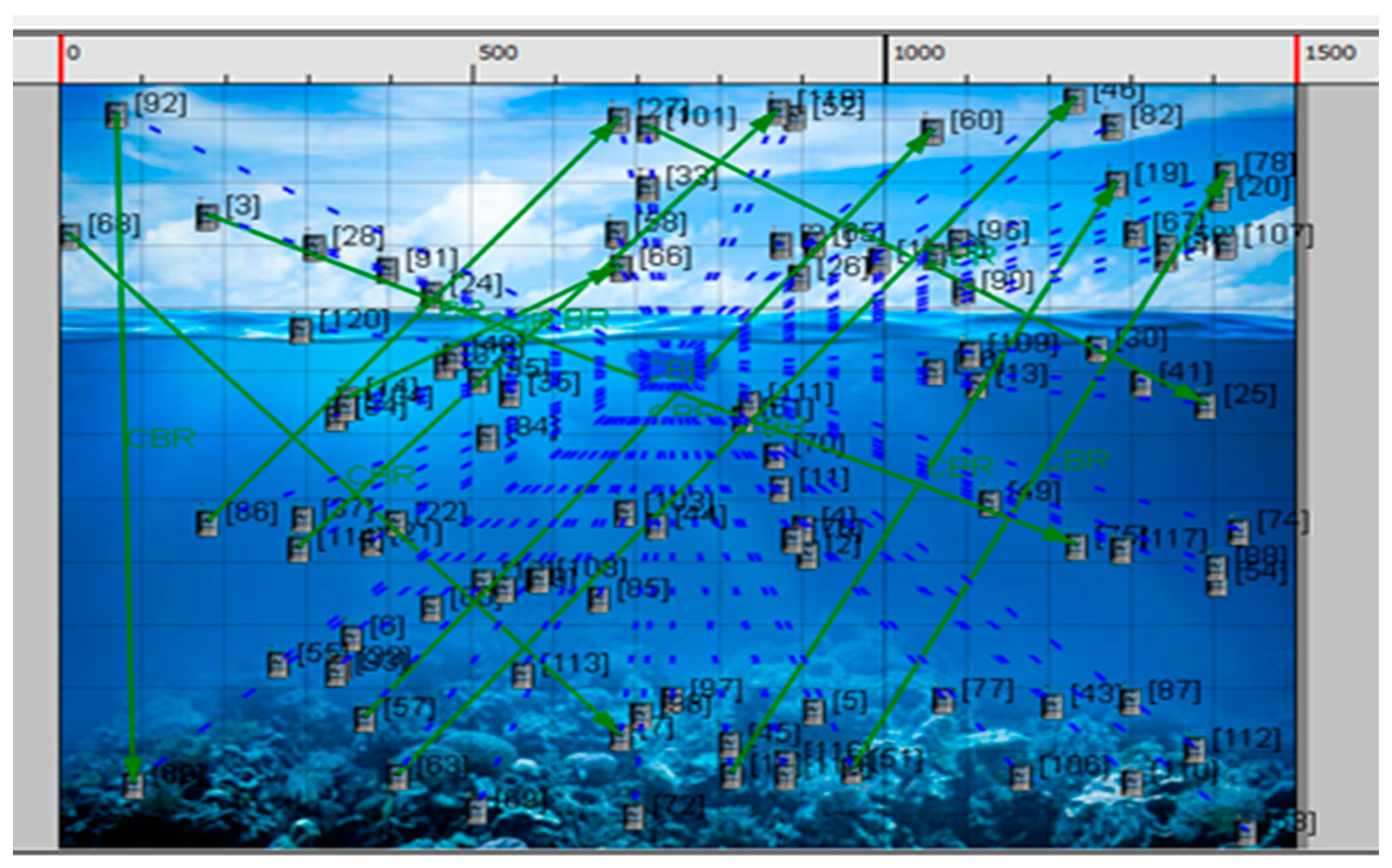
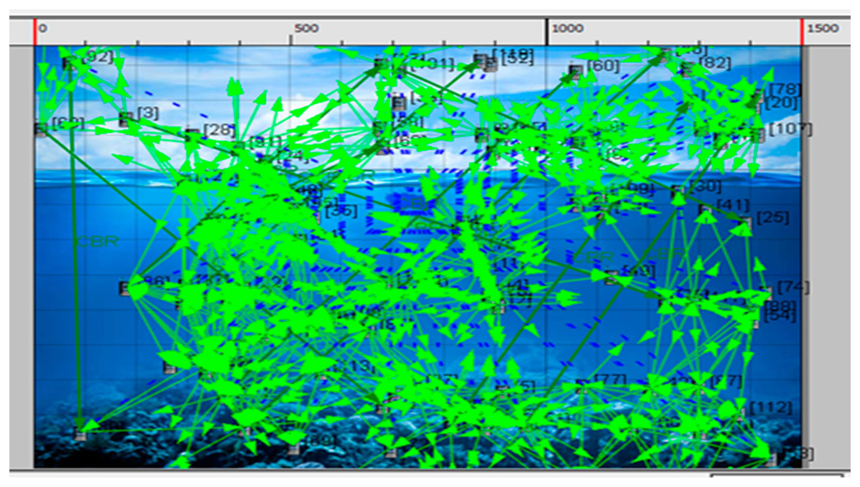
Considering the constant bit rate (CBR) as a deployment application, there are accessible existing networks available. In the proposed network, file transfer protocol (FTP) and variable bitrate (VBR) are considered alongside CBR, and the parameters for all three FTP, CBR, and VBR applications are then compared [35,36]. The proposed scenario has a 1500 × 1500 square meter design in the Qualnet 7.1 Simulator. The FTP, CBR, and VBR applications are connected between 60 and 120 nodes, of which 15 are node devices, 25 are ship devices, 20 are sensor devices for 60 nodes, 30 are node devices, 50 are ship devices and 40 are sensor devices. The simulation lasts for 500 s in total. Random waypoint mobility with a minimum speed of 1.5 m/s and a maximum speed from 3 to 10 m/s is the node mobility model that has been selected. Beyond AODV, the other considered routing protocols are DSR, DYMO, LAR1, Bellman-Ford, OLSR, Fisheye, STAR-ORA, ZRP, and STAR-LORA. After finishing the test, the graphs in the simulator were considered. The required performance metrics are thus obtained, including the average transmission delay, average jitter, percentage of utilization, and the energy used in transmit and receive modes. The proposed underwater wireless communication scenario with multiple nodes in X-Y and 3D visualization is shown in Figure 4 and Figure 5 for 60 nodes. Runtime proposed scenario for underwater wireless communication with various nodes in both X-Y and 3D visualization is shown in Figure 6 and Figure 7 for 120 nodes [37,38].
4. Performance Parameters
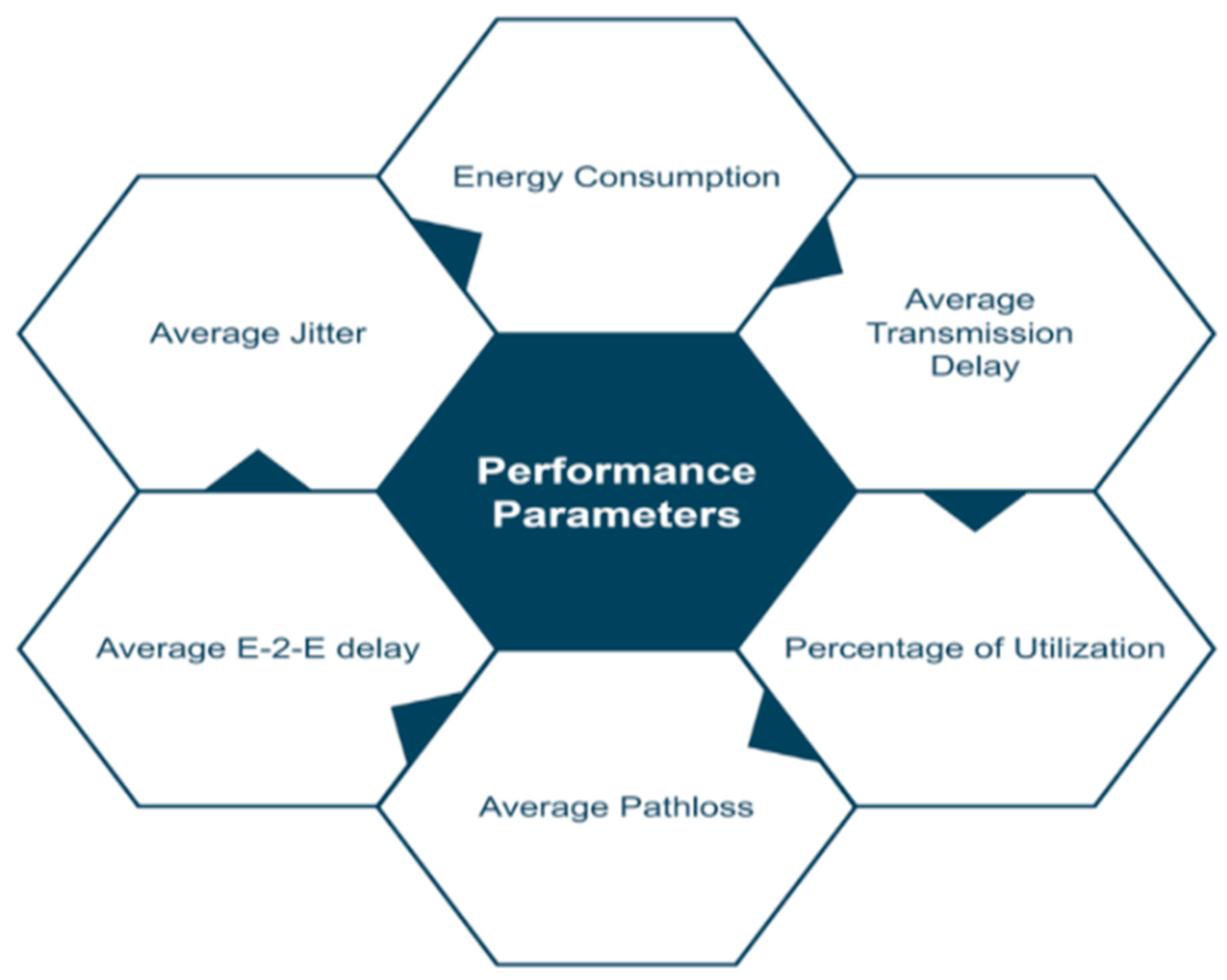
Opnet, Omnet, Matlab, QualNet, and other simulation tools, among others [39,40,41,42], commonly take the design of UWSN into account. The proposed network is created in the QualNet simulator using several user-friendly UWSN design parameters. The performance indicators for the UWSN network in various applications are listed right away and shown in Figure 8.
Energy Consumption: the energy used by nodes to send data from their point of origin to their point of destination.
where Pts denotes the successful packet reception, N is the number of nodes and Etotal is the total energy consumption.
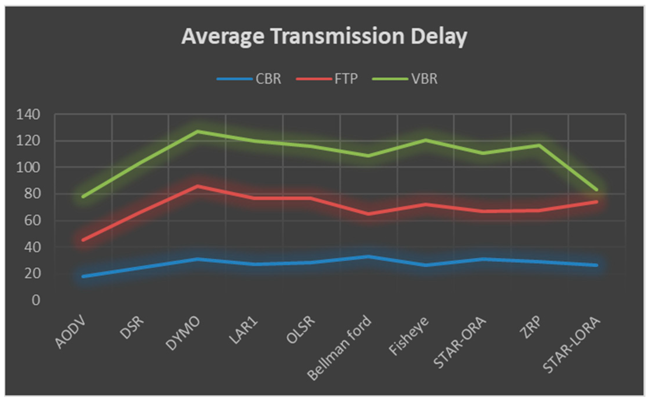
Average Transmission Delay: the average transmission delay is the amount of time it takes for information to successfully travel from its source to its destination.
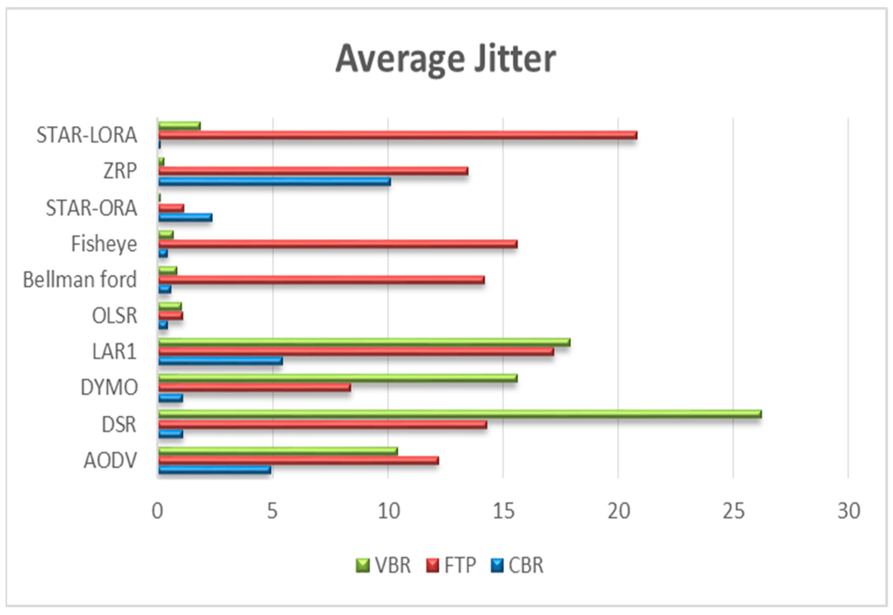
Average Jitter: this measure concerns the time difference between individual packets as a result of route changes or network congestion. A routing protocol should be lower to function more efficiently. A network’s congestion, routing modifications, or timing drift can all increase jitter by delaying the transmission of individual packets.
where Ω = average jitter, = receiver time, = source time.
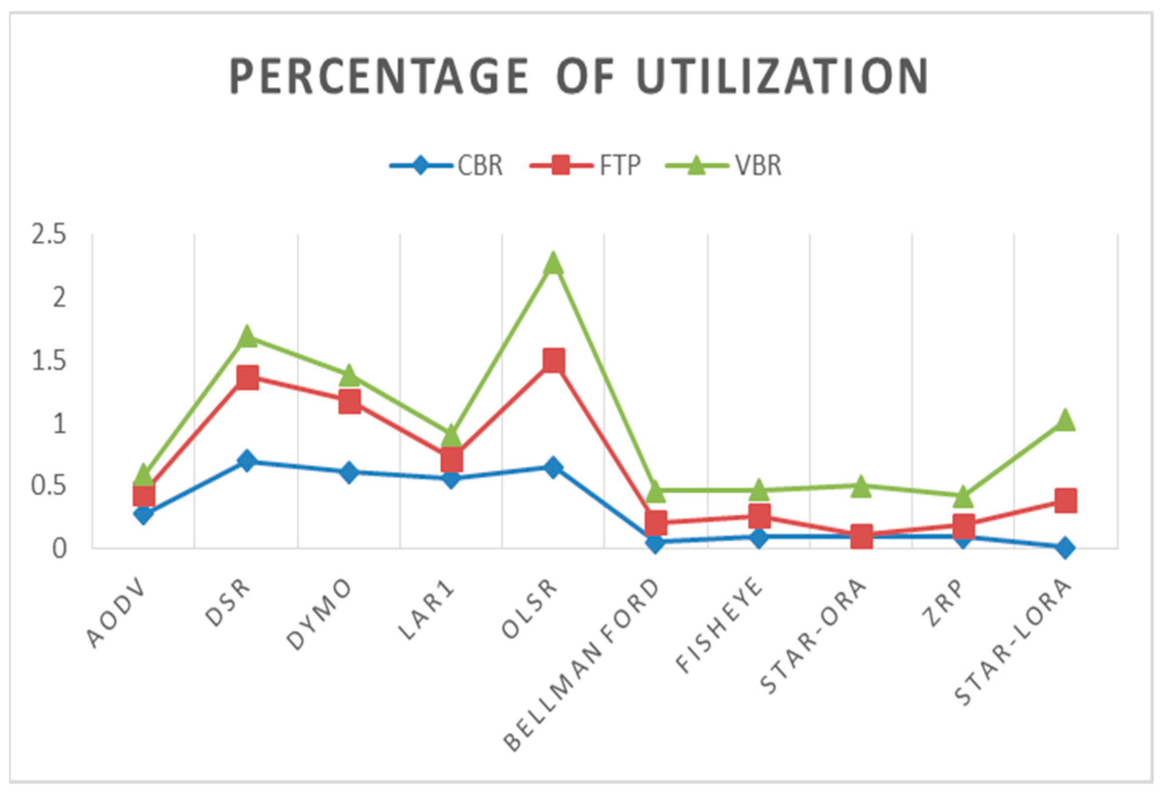
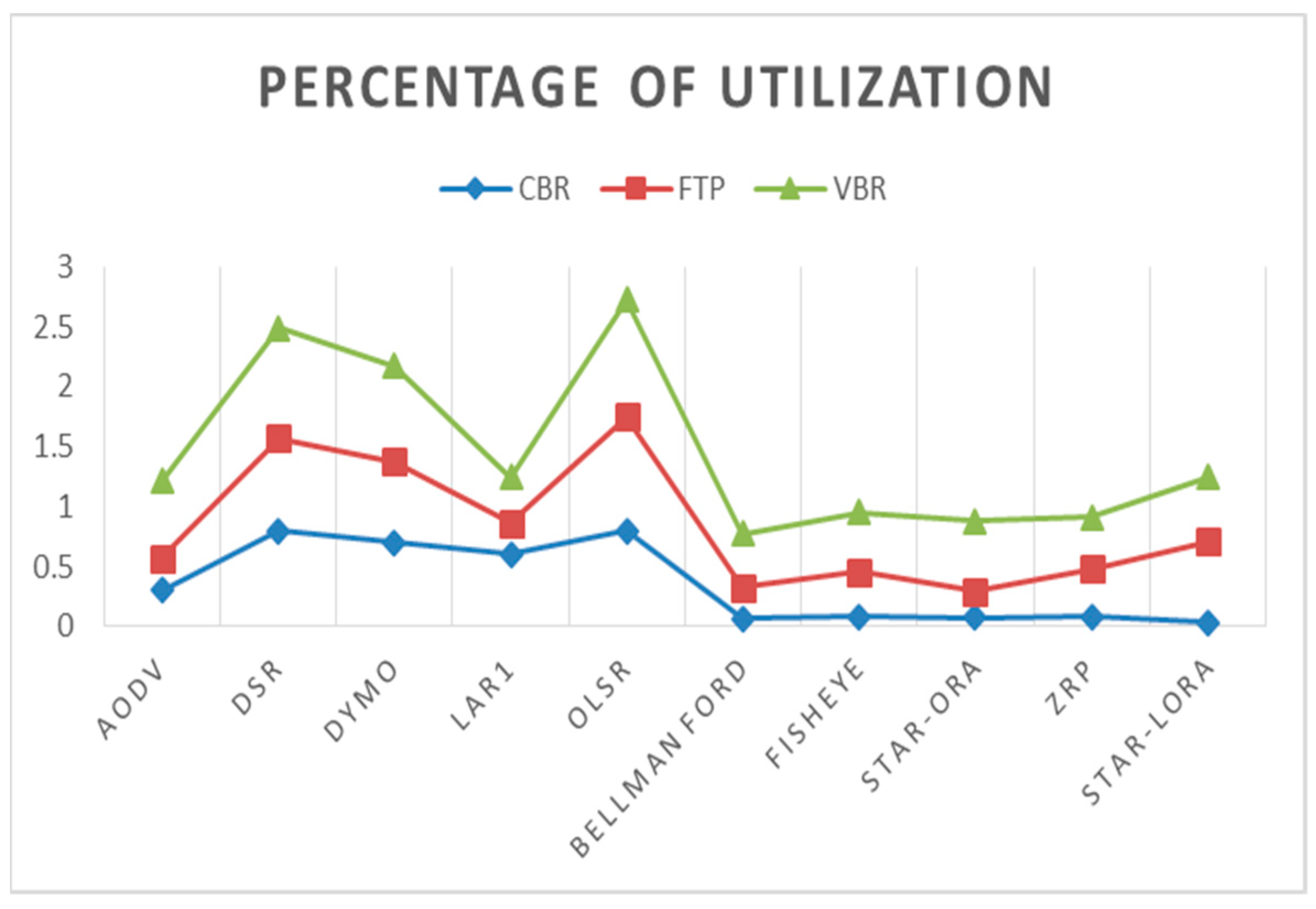
Percentage of Utilization: the proportion of packets that are successfully transferred from the transmitting node to the receiving one is known as the throughput of a communication channel.
where TxPi = packet transmitted by ith node.
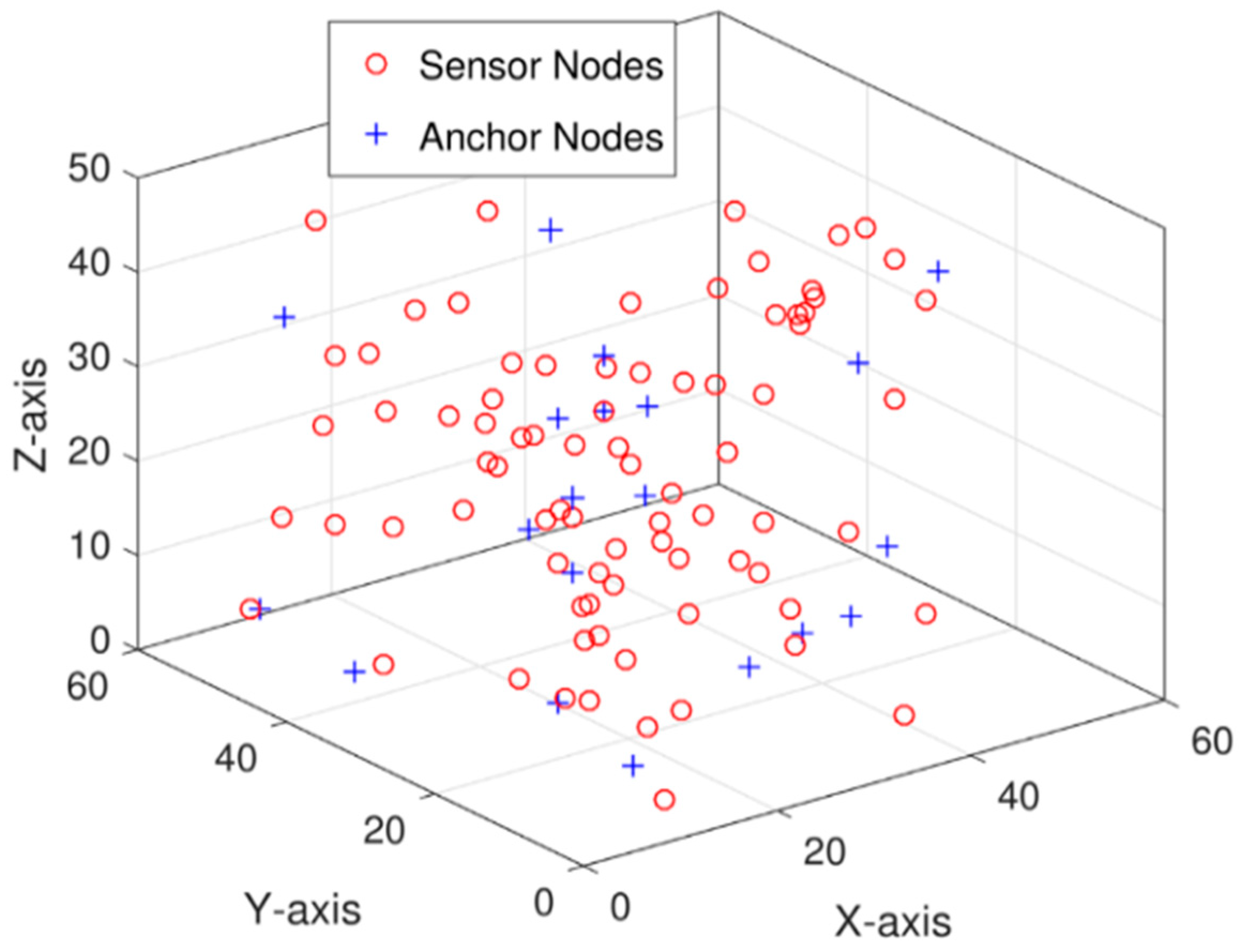
5. Results and Discussion
The deployment of sensor nodes in 3D for the proposed UWSN network scenario, with sensor nodes and anchor nodes, is depicted in Figure 9. Additionally, the investigational results for various routing protocols, including AODV, DSR, DYMO, LAR1, Bellman-Ford, OLSR, Fisheye, STAR-ORA, ZRP, and STAR-LORA with FTP, CBR, and VBR applications, are observed for transmitting and receiving mode power consumption, as displayed in Figure 10 and Figure 11. Figure 10 and Figure 11 show that more power consumption in transmitting and receiving modes is measured in Bellman-Ford, OLSR, and LAR1 routing protocols. The STAR-ORA, ZRP, and STAR-LORA display relatively less power consumption due to the hybrid routing features of these protocols in the UWSN scenario.
Other findings have been obtained from measuring the proposed UWSN network’s performance parameters in FTP, CBR, and VBR applications for deployments of 60 and 120 nodes, respectively. The UWSN network’s performance metrics for FTP, CBR, and VBR applications are as follows.
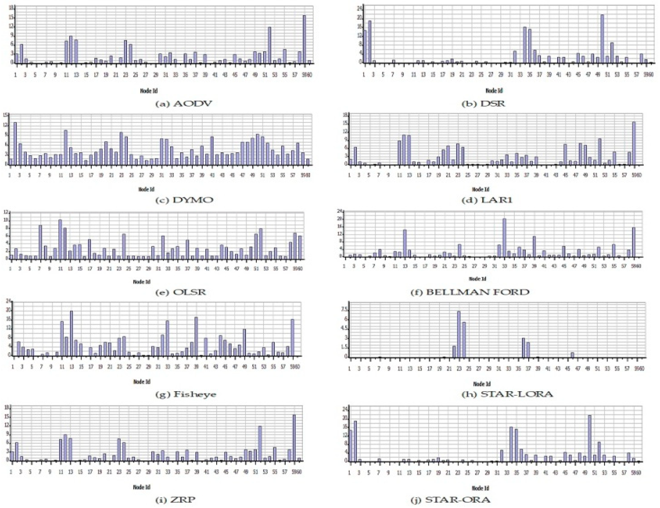
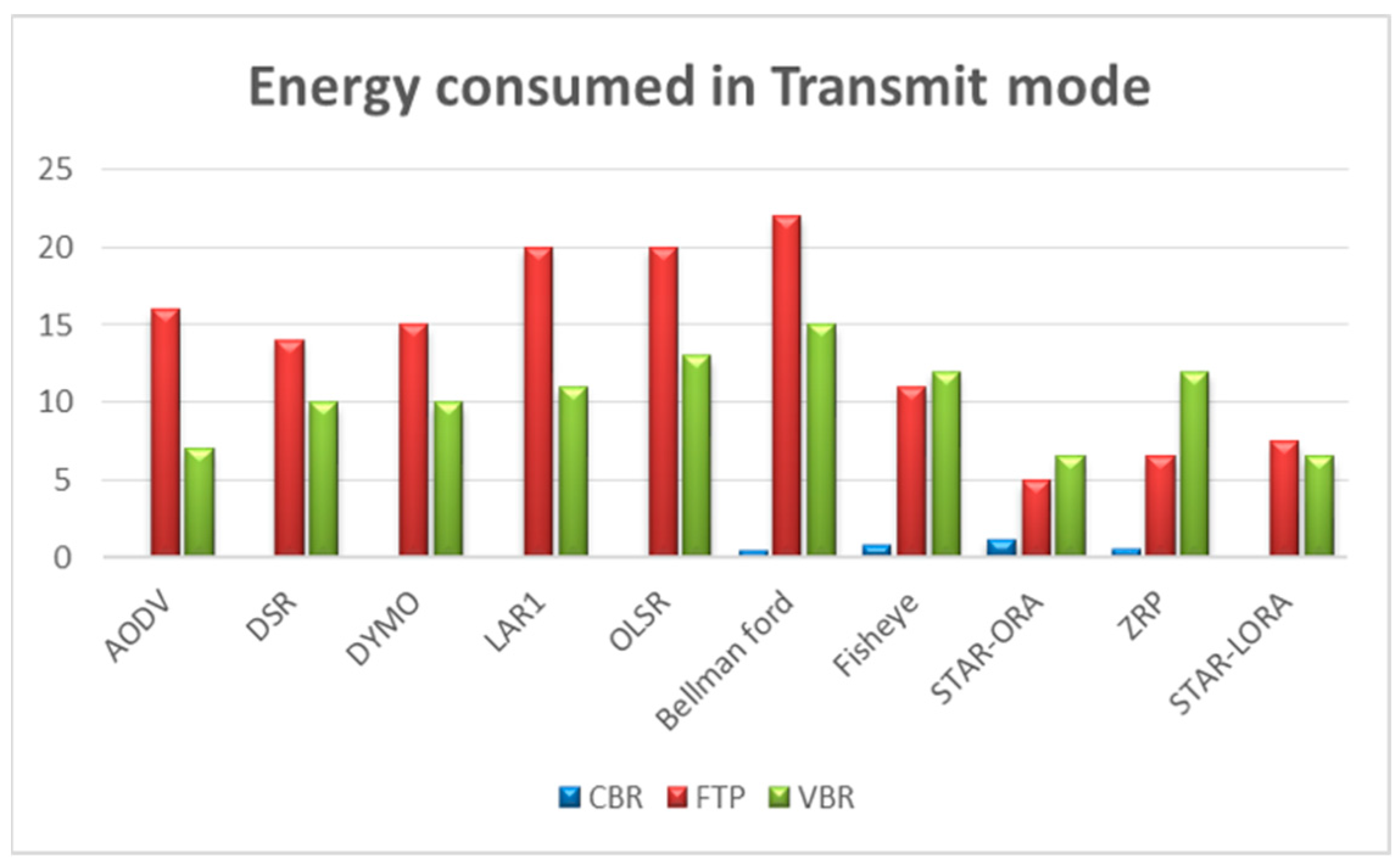
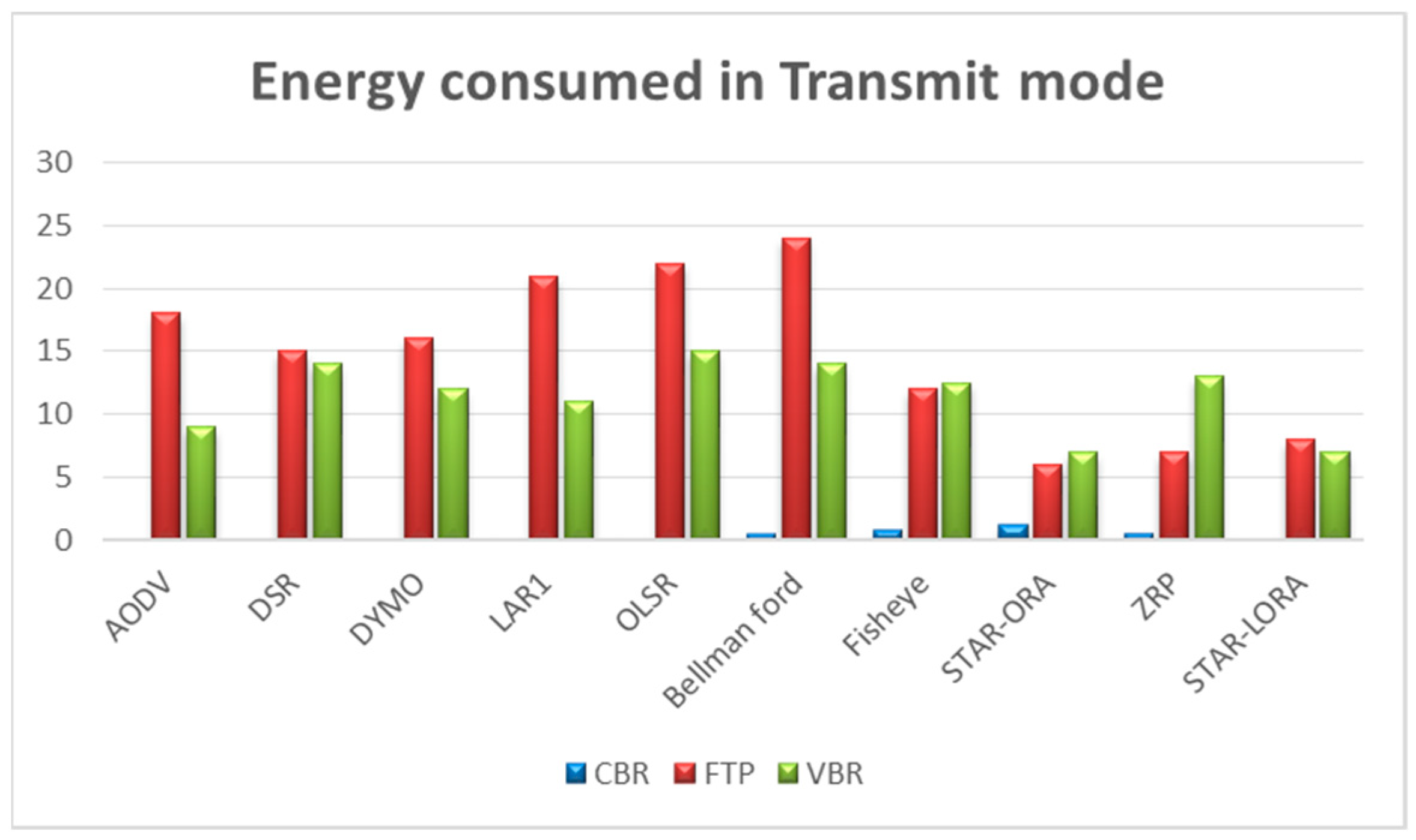
5.1. Energy (mWh) Consumed in Transmit Mode by AODV, DSR, DYMO, LAR1, Bellman-Ford, OLSR, Fisheye, STAR-ORA, ZRP, and STAR-LORA Routing Protocols
The energy consumption in the transmit mode routing protocols of AODV, DSR, DYMO, LAR1, Bellman-Ford, OLSR, Fisheye, STAR-ORA, ZRP, and STAR-LORA with FTP, CBR, and VBR applications for 60 and 120 nodes is pictured in Figure 12 and Figure 13, respectively. Table 1 and Table 2 show the minimum transmit energy required by the DSR, DYMO, LAR1, Bellman-Ford, OLSR, Fisheye, STAR-ORA, ZRP, and STAR-LORA routing protocols to transmit data at their maximum size in the proposed UWSN, i.e., 83.4 percent. The aim of UWSN is the use of as little transmitted energy as possible. Other routing protocols cannot match AODVs speed and dependability.
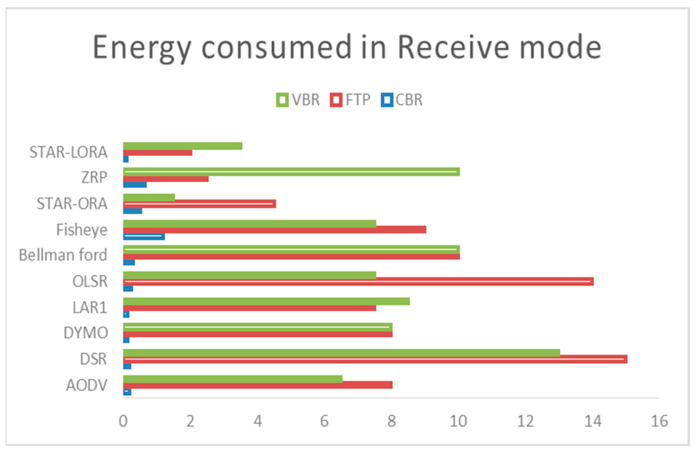
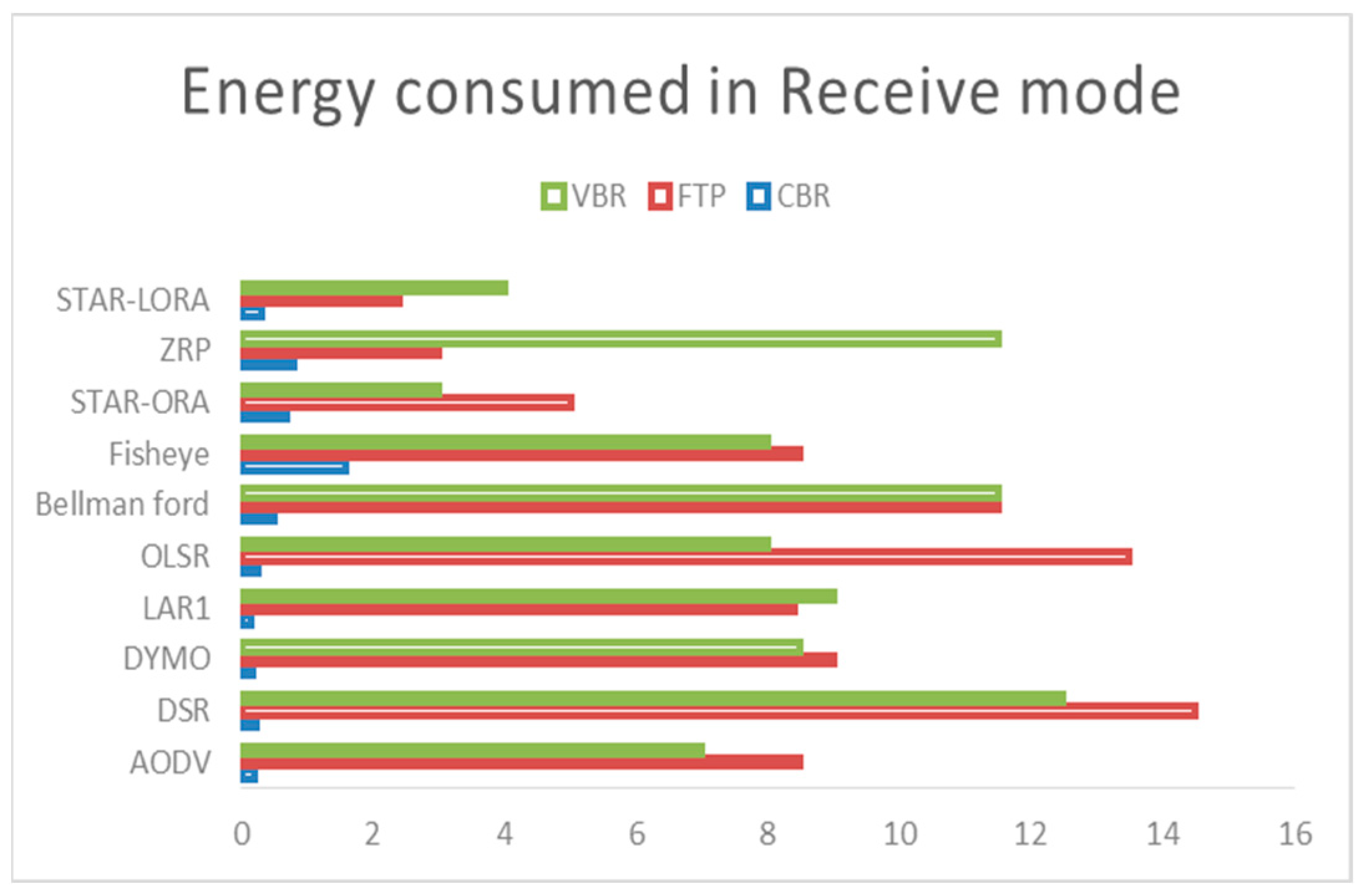
5.2. Energy (mWh) Consumed in Receive Mode by AODV, DSR, DYMO, LAR1, Bellman-Ford, OLSR, Fisheye, STAR-ORA, ZRP and STAR-LORA Routing Protocols
The routing protocols AODV, DSR, DYMO, LAR1, Bellman-Ford, OLSR, Fisheye, STAR-ORA, ZRP, and STAR-LORA are compared in Figure 14 and Figure 15 for the amount of received energy they use with FTP, CBR, and VBR applications for 60 and 120 nodes, respectively.
The AODV routing protocol uses 76.4 percent less receive energy in CBR application than the other routing protocols, as shown in Table 1 and Table 2, including DSR, DYMO, LAR1, Bellman-Ford, OLSR, Fisheye, STAR-ORA, ZRP, and STAR-LORA. When dealing with larger packet sizes than other routing protocols, the AODV routing protocol uses significantly less received energy than those other routing protocols. When receiving data, UWSN should use the least amount of energy possible. Performance-wise, the AODV routing protocol outperforms other routing protocols.
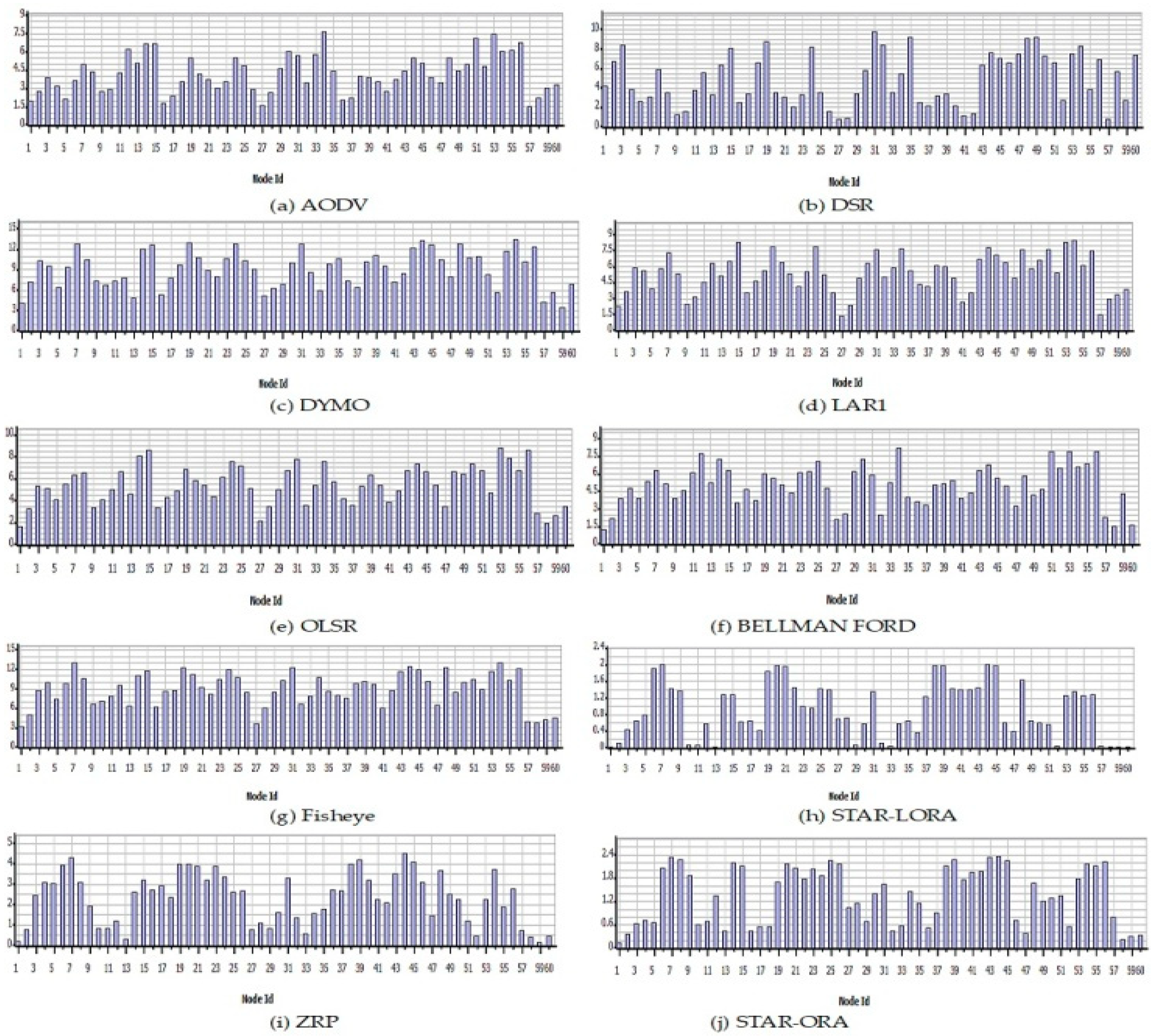
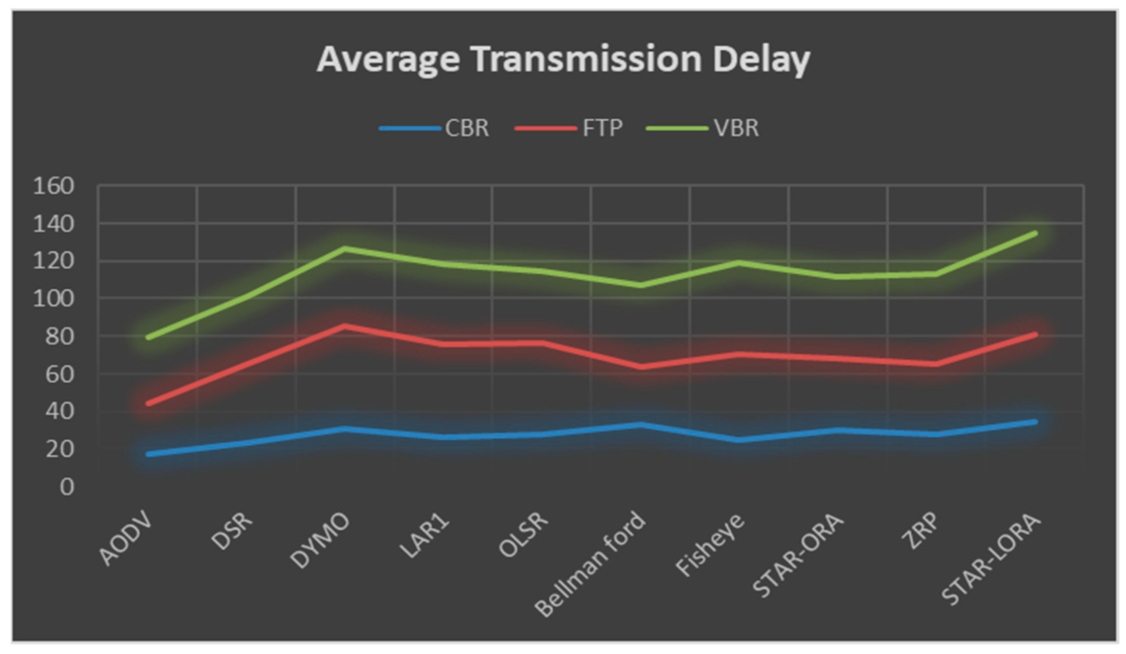
5.3. Average Transmission Delay (µs) by AODV, DSR, DYMO, LAR1, Bellman-Ford, OLSR, Fisheye, STAR-ORA, ZRP and STAR-LORA Routing Protocols
The average delay of AODV, DSR, DYMO, LAR1, Bellman-Ford, OLSR, Fisheye, STAR-ORA, ZRP, and STAR-LORA protocols for 60 and 120 nodes, respectively, are displayed in Figure 16 and Figure 17. As displayed in Table 1 and Table 2, the AODV routing protocol produces an average CBR application delay of 88.6% less than that of other routing protocols.
5.4. Percentage of Utilization by AODV, DSR, DYMO, LAR1, Bellman-Ford, OLSR, Fisheye, STAR-ORA, ZRP, and STAR-LORA Routing Protocols
Table 1 and Table 2 demonstrate that the Fisheye routing protocol outperformed the competition in terms of percentage of utilization for the CBR application (91.4%), and Figure 18 and Figure 19 show percentages of utilization for the following routing protocols: AODV, DSR, DYMO, LAR1, Bellman-Ford, OLSR, Fisheye, STAR-ORA, ZRP, and STAR-LORA.
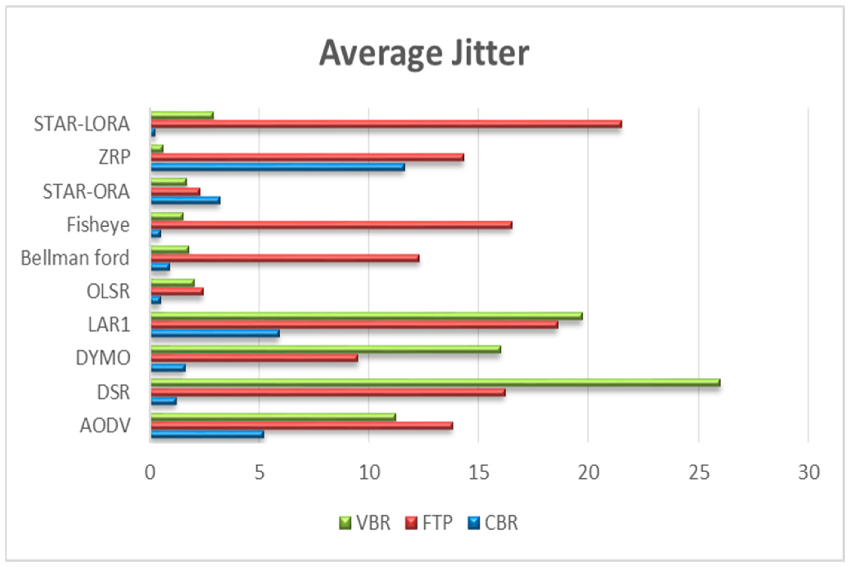
5.5. Average Jitter (µs) by AODV, DSR, DYMO, LAR1, Bellman-Ford, OLSR, Fisheye, STAR-ORA, ZRP, and STAR-LORA Routing Protocols
6. Conclusions
Several aspects are evolving while exploring an underwater environment, such as monitoring underwater resources, investigating parameters, and planning military action. The extent of battery power is the network’s primary focus because UWSN can only carry out specific tasks. This study compares the performance of the routing protocols AODV, DSR, DYMO, LAR1, Bellman-Ford, OLSR, Fisheye, STAR-ORA, ZRP, and STAR-LORA in UWSN networks with variable deployment applications such as FTP, CBR, and VBR for 60 and 120 nodes, respectively. Several metrics were tracked, such as average transmission delay, average jitter, utilization rate, and energy used in transmit and receive modes. The simulation results show that, when compared to the DSR, DYMO, LAR1, Bellman-Ford, OLSR, Fisheye, STAR-ORA, ZRP, and STAR-LORA routing protocols, the AODV routing protocol generates the least overall energy with a slight variation of additional nodes as well as 88.6 percent less average transmission delay. Additionally, compared to the AODV, DSR, DYMO, LAR1, Bellman-Ford, OLSR, Fisheye, STAR-ORA, ZRP, and STAR-LORA routing protocols, the Fisheye routing protocol achieves a 91.4% higher percentage of utilization. The average jitter produced by STAR-LORA is 85.3% lower than that of the other routing protocols for 60 and 120 nodes.
Author Contributions
K.S.; Conceptualization, Data curation, Formal Analysis, Methodology, Software, Writing—original draft; C.V.R.; Supervision, Writing—review & editing, Project administration, Visualization; A.R.; Visualization, Investigation, Formal Analysis, Software; G.P.; Data Curation, Investigation, Resources, Software, Writing—original draft, Methodology. All authors have read and agreed to the published version of the manuscript.
Funding
This research received no external funding.
Data Availability Statement
Not applicable.
Conflicts of Interest
The authors declare no conflict of interest.
Routing Protocols Abbreviations
| Ad-hoc On-demand Distance Vector | (AODV) |
| Zone Routing Protocol | (ZRP) |
| Dynamic Source Routing Protocol | (DSR) |
| Fisheye State Routing | (FSR) |
| Dynamic MANET on Demand Routing Protocol | (DYMO) |
| Location Aided Routing | (LAR) |
| Optimized Link State Routing Protocol | (OLSR) |
| Source Tree Adaptive Routing | (STAR) |
| Source Tree Adaptive Routing-Optimum Routing Approach | (STAR-ORA) |
| Source Tree Adaptive Routing-Least Overhead Routing Approach | (STAR-LORA) |
References
- Ayaz, M.; Baig, I.; Abdullah, A.; Faye, I. A survey on routing techniques in underwater wireless sensor networks. J. Netw. Comput. Appl. 2011, 34, 1908–1927. [Google Scholar] [CrossRef]
- Proakis, J.G.; Sozer, E.M.; Rice, J.A.; Stojanovic, M. Shallow water acoustic networks. IEEE Commun. Mag. 2001, 39, 114–119. [Google Scholar] [CrossRef]
- Heidemann, J.; Ye, W.; Wills, J.; Syed, A.; Li, Y. Research challenges and applications for underwater sensor networking. In Proceedings of the Wireless Communications and Networking Conference (WCNC 2006), IEEE, Las Vegas, NV, USA, 3–6 April 2006; Volume 1, pp. 228–235. [Google Scholar]
- Meratnia, N.; Havinga, P.J.; Casari, P.; Petrioli, C.; Grythe, K.; Husoy, T.; Zorzi, M. CLAM—Collaborative embedded networks for submarine surveillance: An overview. In Proceedings of the OCEANS 2011 IEEE-Spain, IEEE, Santander, Spain, 6–9 June 2011; pp. 1–4. [Google Scholar]
- Fang, S.; Xu, L.D.; Zhu, Y.; Ahati, J.; Pei, H.; Yan, J.; Liu, Z. An integrated system for regional environmental monitoring and management based on internet of things. IEEE Trans. Industr. Inf. 2014, 10, 1596–1605. [Google Scholar] [CrossRef]
- Sozer, E.M.; Stojanovic, M.; Proakis, J.G. Underwater acoustic networks. IEEE J. Ocean. Eng. 2000, 25, 72–83. [Google Scholar] [CrossRef]
- Cui, J.H.; Kong, J.; Gerla, M.; Zhou, S. The challenges of building mobile underwater wireless networks for aquatic applications. IEEE Netw. 2006, 20, 12–18. [Google Scholar]
- Rani, S.; Ahmed, S.H.; Malhotra, J.; Talwar, R. Energy efficient chain based routing protocol for underwater wireless sensor networks. J. Netw. Comput. Appl. 2017, 92, 42–50. [Google Scholar] [CrossRef]
- Bhattacharjya, K.; Alam, S.; De, D. Performance analysis of DYMO, ZRP and AODV routing protocols in a multi hop grid based underwater wireless sensor network. In Proceedings of the 2nd International Conference on Computational Intelligence, Communications and Business Analytics (CICBA), Kalyani, India, 27–28 July 2018; Springer Nature: Singapore, 2019. [Google Scholar] [CrossRef]
- Alam, S.; De, D. Cloud smoke sensing model for AODV, RIP and STAR routing protocols using wireless sensor network in industrial township area. In Proceedings of the 2016 Second International Conference on Research in Computational Intelligence and Communication Networks (ICRCICN), Kolkata, India, 23–25 September 2016. [Google Scholar]
- Bhattacharjya, K.; Alam, S.; De, D. TTCBT: Two tier complete binary tree based wireless sensor network for FSR and LANMAR routing protocols. Microsyst. Technol. 2018, 27, 443–453. [Google Scholar] [CrossRef]
- Wang, K.; Gao, H.; Xu, X.; Jiang, J.; Yue, D. An energy-efficient reliable data transmission scheme for complex environmental monitoring in underwater acoustic sensor networks. IEEE Sens. J. 2016, 16, 4051–4062. [Google Scholar] [CrossRef]
- Han, G.; Jiang, J.; Shu, L.; Guizani, M. An attack-resistant trust model based on multidimensional trust metrics in underwater acoustic sensor network. IEEE Trans. Mob. Comput. 2015, 14, 2447–2459. [Google Scholar] [CrossRef]
- Han, G.; Jiang, J.; Shu, L.; Xu, Y.; Wang, F. Localization algorithms of underwater wireless sensor networks: A survey. Sensors 2012, 12, 2026–2061. [Google Scholar] [CrossRef]
- Lee, S.; Kim, D. Underwater hybrid routing protocol for UWSNs. In Proceedings of the Fifth International Conference on Ubiquitous and Future Networks (ICUFN), IEEE, Da Nang, Vietnam, 2–5 July 2013; pp. 472–475. [Google Scholar]
- Yuan, F.; Zhan, Y.; Wang, Y. Data density correlation degree clustering method for data aggregation in WSN. IEEE Sens. J. 2014, 14, 1089–1098. [Google Scholar] [CrossRef]
- Agarwal, R.; Kumar, S.; Hegde, R.M. Algorithms for crowd surveillance using passive acoustic sensors over a multimodal sensor network. IEEE Sens. J. 2015, 15, 1920–1930. [Google Scholar] [CrossRef]
- Ravikumar, C.V.; Bagadi, K.P. Design of MC-CDMA receiver using RBF network to mitigate MAI and nonlinear distortion. Neural Comput. Appl. 2019, 31, 1263–1273. [Google Scholar]
- Perkins, C.; Belding-Royer, E.; Das, S. Ad Hoc On-Demand Distance Vector (AODV) Routing; No. RFC 3561; University of Cincinnati: Cincinnati, OH, USA, 2003. [Google Scholar]
- Teja, G.S.; Samundiswary, P. Performance analysis of DYMO protocol for IEEE 802.15. 4 based WSNs with mobile nodes. In Proceedings of the Computer Communication and Informatics (ICCCI), IEEE, Coimbatore, India, 3–5 January 2014; pp. 1–5. [Google Scholar]
- Park, M.K.; Rodoplu, V. UWAN-MAC: An energy-efficient MAC protocol for underwater acoustic wireless sensor networks. IEEE J. Ocean. Eng. 2007, 32, 710–720. [Google Scholar] [CrossRef]
- Rani, S.; Talwar, R.; Malhotra, J.; Ahmed, S.H.; Sarkar, M.; Song, H. A novel scheme for an energy efficient Internet of Things based on wireless sensor networks. Sensors 2015, 15, 28603–28626. [Google Scholar] [CrossRef] [PubMed] [Green Version]
- Domingo, M.C.; Prior, R. Energy analysis of routing protocols for underwater wireless sensor networks. Comput. Commun. 2008, 31, 1227–1238. [Google Scholar] [CrossRef]
- Ravikumar, C.V.; Bagadi, K.P. MC-CDMA receiver design using recurrent neural network for eliminating MAI and nonlinear distortion. Int. J. Commun. Syst. IJCS 2017, 30, e3328. [Google Scholar]
- Patil, M.S.A.; Mishra, M.P. Improved mobicast routing protocol to minimize energy consumption for underwater wireless sensor networks. Int. J. Res. Sci. Eng. 2017, 3, 197–204. [Google Scholar]
- Khan, A.; Ahmedy, I.; Anisi, M.H.; Javaid, N.; Ali, I.; Khan, N.; Alsaqer, M.; Mahmood, H. A localization-free interference and energy holes minimization routing for underwater wireless sensor networks. Sensors 2018, 18, 165. [Google Scholar] [CrossRef] [Green Version]
- Manjula, S.H.; Abhilash, C.N.; Shaila, K.; Venugopal, K.R.; Patnaik, L.M. Performance of AODV routing protocol using group and entity mobility models in wireless sensor networks. In Proceedings of the International Multi Conference of Engineers and Computer Scientist, Hong Kong, 19–21 March 2008; Volume 2, pp. 1212–1217. [Google Scholar]
- Khan, A.; Ali, I.; Rahman, A.U.; Imran, M.; Mahmood, H. CoEEORS: Cooperative energy efficient optimal relay selection pr otocol for underwater wireless sensor networks. IEEE Access 2018, 6, 28777–28789. [Google Scholar] [CrossRef]
- Alkindi, Z.; Alzeidi, N.; Touzene, B.A.A. Performance evolution of grid based routing protocol for underwater wireless sensor networks under different mobile models. Int. J. Wirel. Mob. Netw. IJWMN 2018, 10, 13–25. [Google Scholar]
- Wang, Z.; Han, G.; Qin, H.; Zhang, S.; Sui, Y. An energy-aware and void-avoidable routing protocol for underwater sensor networks. IEEE Access 2018, 6, 7792–7801. [Google Scholar] [CrossRef]
- Yildiz, H.U.; Gungor, V.C.; Tavli, B. Packet size optimization for lifetime maximization in underwater acoustic sensor networks. IEEE Trans. Ind. Inform. 2018, 15, 719–729. [Google Scholar] [CrossRef]
- Emokpae, L.E.; DiBenedetto, S.; Potteiger, B.; Younis, M. UREAL: Underwater reflection enabled acoustic-based localization. IEEE Sens. J. 2014, 14, 3915–3925. [Google Scholar] [CrossRef]
- Liang, Q.; Zhang, B.; Zhao, C.; Pi, Y. TDoA for passive localization: Underwater versus terrestrial environment. IEEE Trans. Parallel Distrib. Syst. 2013, 24, 2100–2108. [Google Scholar] [CrossRef]
- Yu, Z.; Xiao, C.; Zhou, G. Multi-objectification-based localization of underwater sensors using magnetometers. IEEE Sens. J. 2014, 14, 1099–1106. [Google Scholar] [CrossRef]
- Diamant, R.; Lampe, L. Underwater localization with time-synchronization and propagation speed uncertainties. IEEE Trans. Mob. Comput. 2013, 12, 1257–1269. [Google Scholar] [CrossRef]
- Varshney, P.K.; Agrawal, G.S.; Sharma, S.K. Relative performance analysis of proactive routing protocols in wireless ad hoc networks using varying node density. Invertis. J. Sci. Technol. 2016, 9, 161–169. [Google Scholar] [CrossRef]
- Bhattacharya, K.; Alam, S.; De, D. CUWSN: Energy efficient routing protocol selection for cluster-based underwater wireless sensor network. Microsyst. Technol. 2019, 28, 543–559. [Google Scholar] [CrossRef]
- Alsulami, M.; Elfouly, R.; Ammar, R. A reliable underwater computing system. In Proceedings of the 2021 4th IEEE International Conference on Industrial Cyber-Physical Systems (ICPS), Victoria, BC, Canada, 10–12 May 2021; pp. 467–472. [Google Scholar]
- Subramani, N.; Mohan, P.; Alotaibi, Y.; Alghamdi, S.; Khalaf, O.I. An Efficient Metaheuristic-Based Clustering with Routing Protocol for Underwater Wireless Sensor Networks. Sensors 2022, 22, 415. [Google Scholar] [CrossRef]
- Ba, X.; Jin, L.; Li, Z.; Du, J.; Li, S. Multiservice-Based Traffic Scheduling for 5G Access Traffic Steering, Switching and Splitting. Sensors 2022, 22, 3285. [Google Scholar] [CrossRef] [PubMed]
- Mohan, P.; Subramani, N.; Alotaibi, Y.; Alghamdi, S.; Khalaf, O.I.; Ulaganathan, S. Improved Metaheuristics-Based Clustering with Multihop Routing Protocol for Underwater Wireless Sensor Networks. Sensors 2022, 22, 1618. [Google Scholar] [CrossRef] [PubMed]
- Sathish, K.; Ravikumar, C.V.; Srinivasulu, A.; Anand Kumar, G. Performance Analysis of Underwater Wireless Sensor Network by Deploying FTP, CBR, and VBR as Applications. J. Comput. Netw. Commun. 2022, 2022, 7143707. [Google Scholar] [CrossRef]
Figure 1.
Typical underwater wireless communication structure.

Figure 2.
3D- Visualization of underwater wireless communication.

Figure 3.
Internal architecture of sensor networks for underwater wireless communication.

Figure 4.
Proposed scenario of underwater wireless communication in X-Y visualization.

Figure 5.
Runtime 3D scenario of underwater wireless communication 3D visualization.

Figure 6.
Proposed underwater wireless communication with 120 nodes in X-Y visualization.

Figure 7.
Runtime underwater wireless communication with 120 nodes in X-Y visualization.

Figure 8.
Performance parameters of UWSN.

Figure 9.
Deployment of sensor nodes in 3D for the proposed underwater wireless sensor network.

Figure 10.
Transmit mode power consumption (mWh) for various routing protocols.

Figure 11.
Receive mode power consumption (mWh) for various routing protocols.

Figure 12.
Transmit mode energy consumption of all routing protocols for 60 nodes.

Figure 13.
Transmit mode energy consumption of all routing protocols for 120 nodes.

Figure 14.
Receive mode energy consumption of all routing protocols for 60 nodes.

Figure 15.
Receive mode energy consumption of all routing protocols for 120 nodes.

Figure 16.
Average transmission delay of all routing protocols for 60 nodes.

Figure 17.
Average transmission delay of all routing protocols for 120 nodes.

Figure 18.
Percentage of utilization of all routing protocols for 60 nodes.

Figure 19.
Percentage of utilization of all routing protocols for 120 nodes.

Figure 20.
Average jitter of all routing protocols for 60 nodes.

Figure 21.
Average jitter of all routing protocols for 120 nodes.


Table 1.
Comparison of all routing protocols for 60 nodes.
| Parameter | Protocol | |||||||||||||||||||||||||||||
|---|---|---|---|---|---|---|---|---|---|---|---|---|---|---|---|---|---|---|---|---|---|---|---|---|---|---|---|---|---|---|
| OLSR | DSR | AODV | LAR1 | DYMO | ZRP | STAR-LORA | STAR-ORA | FISHEYE | BELLMAN FORD | |||||||||||||||||||||
| CBR | FTP | VBR | CBR | FTP | VBR | CBR | FTP | VBR | CBR | FTP | VBR | CBR | FTP | VBR | CBR | FTP | VBR | CBR | FTP | VBR | CBR | FTP | VBR | CBR | FTP | VBR | CBR | FTP | VBR | |
| Average transmission delay (µs) | 28 | 49 | 39 | 23 | 42 | 36 | 18 | 27 | 35 | 27 | 49 | 43 | 31 | 55 | 41 | 28 | 38 | 48 | 35 | 46 | 54 | 30 | 38 | 44 | 25 | 46 | 48 | 33 | 31 | 44 |
| Receive power consumption (mWh) | 0.2 | 14 | 7.5 | 0.2 | 15 | 13 | 0.2 | 8 | 6.5 | 0.1 | 14 | 8.5 | 0.1 | 8 | 8 | 0.7 | 2.5 | 10 | 0.1 | 2 | 3.5 | 0.5 | 4.5 | 1.5 | 1.2 | 9 | 7.5 | 0.3 | 10 | 10 |
| Transmit power consumption (mWh) | 0.1 | 20 | 13 | 0.1 | 14 | 10 | 0.1 | 16 | 7 | 0.1 | 20 | 11 | 0.1 | 15 | 10 | 0.6 | 6.5 | 12 | 0.1 | 7.5 | 6.5 | 1.2 | 5 | 6.5 | 0.8 | 11 | 12 | 0.5 | 22 | 15 |
| Percentage of utilization | 0.7 | 0.9 | 0.8 | 0.7 | 0.7 | 0.3 | 0.3 | 0.2 | 0.1 | 0.6 | 0.2 | 0.2 | 0.6 | 0.6 | 0.2 | 0.1 | 0.1 | 0.2 | 0 | 0.4 | 0.7 | 0.1 | 0 | 0.2 | 0.1 | 0.2 | 0.2 | 0.1 | 0.2 | 0.3 |
| Average jitter (µs) | 0.4 | 1.1 | 1 | 1.4 | 14 | 26 | 4.9 | 12 | 10 | 5.4 | 17 | 18 | 1.1 | 8.4 | 16 | 10 | 14 | 0.3 | 0.1 | 21 | 1.9 | 2.4 | 1.1 | 0.1 | 0.4 | 16 | 0.7 | 0.6 | 14 | 0.8 |
Table 2.
Comparison of all routing protocols for 120 nodes.
| Parameter | Protocol | |||||||||||||||||||||||||||||
|---|---|---|---|---|---|---|---|---|---|---|---|---|---|---|---|---|---|---|---|---|---|---|---|---|---|---|---|---|---|---|
| OLSR | DSR | AODV | LAR1 | DYMO | ZRP | STAR-LORA | STAR-ORA | FISHEYE | BELLMAN-FORD | |||||||||||||||||||||
| CBR | FTP | VBR | CBR | FTP | VBR | CBR | FTP | VBR | CBR | FTP | VBR | CBR | FTP | VBR | CBR | FTP | VBR | CBR | FTP | VBR | CBR | FTP | VBR | CBR | FTP | VBR | CBR | FTP | VBR | |
| Average transmission delay (µs) | 28 | 49 | 39 | 24 | 42 | 37 | 18 | 27 | 33 | 27 | 50 | 43 | 31 | 55 | 41 | 29 | 38 | 49 | 26 | 48 | 54 | 31 | 36 | 44 | 26 | 46 | 48 | 33 | 32 | 44 |
| Receive power consumption (mWh) | 0.3 | 14 | 8 | 0.2 | 15 | 13 | 0.2 | 8.5 | 7 | 0.1 | 8.4 | 9 | 0.2 | 9 | 8.5 | 0.8 | 3 | 12 | 0.3 | 2.4 | 4 | 0.7 | 5 | 3 | 1.6 | 8.5 | 8 | 0.5 | 12 | 11 |
| Transmit power consumption (mWh) | 0.1 | 22 | 15 | 0.2 | 15 | 14 | 0.1 | 18 | 9 | 0.1 | 21 | 12 | 0.1 | 16 | 12 | 0.6 | 7 | 13 | 0.2 | 8 | 7 | 1.2 | 5 | 6.5 | 0.8 | 12 | 13 | 0.5 | 24 | 16 |
| Percentage of utilization | 0.8 | 1 | 1 | 0.8 | 0.8 | 0.9 | 0.3 | 0.3 | 0.6 | 0.6 | 0.3 | 0.4 | 0.7 | 0.7 | 0.8 | 0.1 | 0.4 | 0.4 | 0 | 0.7 | 0.7 | 0.1 | 0.2 | 0.6 | 0.1 | 0.4 | 0.5 | 0.1 | 0.3 | 0.5 |
| Average jitter (µs) | 0.5 | 2.4 | 2 | 1.2 | 16 | 26 | 5.2 | 14 | 11 | 5.9 | 19 | 20 | 1.6 | 9.5 | 16 | 12 | 14 | 0.6 | 0.3 | 22 | 2.9 | 3.2 | 2.3 | 1.7 | 0.5 | 17 | 1.5 | 0.9 | 12 | 1.8 |
Publisher’s Note: MDPI stays neutral with regard to jurisdictional claims in published maps and institutional affiliations. |
© 2022 by the authors. Licensee MDPI, Basel, Switzerland. This article is an open access article distributed under the terms and conditions of the Creative Commons Attribution (CC BY) license (https://creativecommons.org/licenses/by/4.0/).
Share and Cite
MDPI and ACS Style
Sathish, K.; Ravikumar, C.V.; Rajesh, A.; Pau, G. Underwater Wireless Sensor Network Performance Analysis Using Diverse Routing Protocols. J. Sens. Actuator Netw. 2022, 11, 64. https://doi.org/10.3390/jsan11040064
AMA Style
Sathish K, Ravikumar CV, Rajesh A, Pau G. Underwater Wireless Sensor Network Performance Analysis Using Diverse Routing Protocols. Journal of Sensor and Actuator Networks. 2022; 11(4):64. https://doi.org/10.3390/jsan11040064
Chicago/Turabian StyleSathish, Kaveripaka, Chinthaginjala Venkata Ravikumar, Anbazhagan Rajesh, and Giovanni Pau. 2022. "Underwater Wireless Sensor Network Performance Analysis Using Diverse Routing Protocols" Journal of Sensor and Actuator Networks 11, no. 4: 64. https://doi.org/10.3390/jsan11040064
Note that from the first issue of 2016, this journal uses article numbers instead of page numbers. See further details here.