
Expansionary Monetary Policy and Bank Loan Loss Provisioning
by
 ,
,
Mengyang Guo
1, 
Xiaoran Jia
2,
Justin Yiqiang Jin
1,
Kiridaran Kanagaretnam
3,* and
Gerald J. Lobo
4 1
DeGroote School of Business, McMaster University, Hamilton, ON L8S 4L8, Canada
2
Lazaridis School of Business, Wilfrid Laurier University, Waterloo, ON N2L 3C5, Canada
3
Schulich School of Business, York University, Toronto, ON M3J 1P3, Canada
4
C. T. Bauer College of Business, University of Houston, Houston, TX 77058, USA
*
Author to whom correspondence should be addressed.
J. Risk Financial Manag. 2024, 17(1), 8; https://doi.org/10.3390/jrfm17010008
Submission received: 4 November 2023
/
Revised: 12 December 2023
/
Accepted: 15 December 2023
/
Published: 22 December 2023
(This article belongs to the Special Issue The Effects of Interest Rates and Macroprudential Policies on Banks' Credit Portfolio)
Abstract
:We explore how expansionary monetary policy (EMP) influences bank loan loss provisioning. We find that banks’ discretionary loan loss provisions (DLLPs) increase during periods of EMP. This effect is stronger for banks with greater risk-taking, a larger proportion of influential stakeholders, lower ex-ante transparency of loan loss provisions, and more stringent bank regulation, which is consistent with external stakeholders requiring more conservative and timelier loan loss provisioning. We also find that both the timeliness and the validity of banks’ loan loss provisions (LLPs) increase during EMP periods. Our results are robust to the use of instrumental variable estimation and exogenous variations in monetary policy. Lastly, we show that conservative (i.e., higher DLLPs) and timely loan loss provisioning discipline banks from excessive risk-taking during periods of EMP.
Keywords:
expansionary monetary policy; loan loss provisions; loan loss provision timeliness; conservative loan loss accountingJEL Classification:
E50; G21; G32; M41; M41. Introduction
Although expansionary monetary policy (EMP) is intended to stimulate economic growth and rebuild consumer confidence (Delis and Kouretas 2011), it can also have a destabilizing effect on financial institutions (Stein 2014; Dang 2022a, 2022b). Academics and the business press have expressed concern that EMP fuels a boom in asset prices and securitized credit, thereby leading financial institutions to increase their lending by more than they usually would through traditional transmission mechanisms.1 Consistent with this view, prior literature suggests that banks can take on higher leverage and engage in riskier lending during periods of EMP (Nichols et al. 2009; Maddaloni and Peydro 2011; Farhi and Tirole 2012; Chodorow-Reich 2014; Dell’Ariccia et al. 2017; Soenen and Vennet 2022). We hypothesize that because bank managers have incentives to take on excessive risks and to use income-increasing accounting discretion to avoid earnings declines or to meet/beat benchmarks during periods of EMP, external stakeholders are likely to demand more conservative and timelier loan loss accounting.
EMP could increase agency costs between bank managers and external stakeholders for the following three reasons. First, a low interest rate decreases the return on safe assets and the hurdle rate on risky assets, causing banks to re-allocate assets from safer assets to riskier assets (Fishburn and Porter 1976; Chodorow-Reich 2014), increasing bank managers’ incentive to take on excessive risk (Grimm et al. 2023). Second, EMP relaxes banks’ borrowing constraints, leading to more lending (e.g., Bernanke and Blinder 1988, 1992; Kashyap et al. 1993; Kashyap and Stein 1994; Bernanke and Gertler 1995). Such increased lending, together with the lower hurdle rate on riskier assets, could induce bank managers to make excessively risky loans. Third, EMP could increase a bank’s overall cost of funding and decrease its profits because of the maturity mismatch on the bank’s balance sheet (Alessandri and Nelson 2015). For example, Claessens et al. (2018) document that a one-percent decrease in interest rate is associated with an 8-bps drop in banks’ net interest margin.2 The lower bank profitability could incentivize bank managers to use income-increasing accounting discretion to avoid earnings declines or to meet/beat earnings benchmarks (Beatty et al. 2002).
Therefore, during EMP periods, banks can be incentivized to take on excessive risks and expropriate wealth from their stakeholders, with such incentives heightened by the implicit guarantee of government bailout (e.g., Keeley 1990). Anticipating such higher agency costs during EMP periods, external stakeholders will demand more conservative and timelier loan loss accounting to constrain managers’ opportunism and optimistic bias in financial reporting (Watts 2003; Nichols et al. 2009; Jackson and Liu 2010; Bushman and Williams 2012). The principle of accounting conservatism is viewed as requiring higher verification standards for recognizing good news than for recognizing bad news (Basu 1997). For banks, such timely recognition of earnings declines through higher LLP would directly impact their profitability and capital ratios, which, in turn, could affect regulators’ monitoring stringency.3 Consequently, the level of accounting conservatism could affect the ability of banks to take excessive risk. For instance, Watts and Zuo (2011) document that banks that report conservatively also tend to take less risks. In addition, regulators, concerned about the excessive risk-taking of banks during EMP periods, may anticipate a capital crunch problem4 if banks do not set aside sufficient loan loss reserves (Laeven and Majnoni 2003; Beatty and Liao 2011). In this sense, EMP should be positively related to more conservative income-decreasing discretionary loan loss provisions (DLLPs) and the timeliness of loan loss provisioning.
We examine the relationship between EMP and banks’ DLLPs for a large sample of 14,623 public bank quarters in the U.S. from 1995Q1 to 2010Q4. Our primary measure of EMP is the Boschen–Mills (BM) index, which distinguishes expansionary from contractionary policy stances (Boschen and Mills 1995; Weise 2008; Lo 2015). Specifically, a BM index of 1 or 2 indicates expansionary periods, with 2 signifying strongly expansionary; a BM index of −2, −1, or 0 indicates non-expansionary periods, with −2 signifying strongly contractionary. Our secondary measure of EMP is the federal funds rate (FFR), which is the target overnight interest rate set by the Federal Open Market Committee (FOMC). Consistent with our reasoning that banks’ external stakeholders require more conservative and timelier loan loss accounting due to the higher agency costs between bank managers and external stakeholders during EMP periods, we find that banks’ income-decreasing DLLP is positively associated with EMP. This effect is also economically significant. Using the BM index (FFR) as the measure of EMP, a one-standard deviation increase in EMP is associated with a 7.78% (24.15%) increase in LLP. In addition, we find that both the timeliness and the validity of banks’ LLP are higher during periods of EMP. Using the BM index as the measure of EMP, we document that the positive relation between the current period LLP and future periods’ change in non-performing loans (or future periods’ net loan charge-offs) is stronger during EMP periods. These results are consistent with the findings of prior studies that banks exhibit greater conservatism in loan loss accounting by recording larger and timelier loan loss provisions (e.g., Nichols et al. 2009).
We perform several cross-sectional tests to support our reasoning that EMP is positively related to income-decreasing DLLP through the channel of external stakeholders’ demanding more conservative and timelier loan loss accounting. We find that the relationship between EMP and income-decreasing DLLP is stronger for banks that have a higher level of risk-taking, a larger proportion of institutional ownership, lower ex-ante informativeness of loan loss provisions, and more stringent bank regulation. These findings suggest that banks that are more incentivized to practice conservative and timelier loan loss accounting are more likely to report higher DLLPs during periods of EMP. To further corroborate our reasoning, we employ path analysis and find that the relation between EMP and DLLP is positively mediated by the inter-temporal change in bank risk.
We conduct several additional analyses to strengthen the internal validity of our main findings, which are predicated on the exogeneity of EMP. However, EMP could be endogenous to business cycles and the associated macroeconomic fundamentals, which also influence banks’ LLP. We address this concern in four ways. First, we employ instrumental variable estimation to control for potential endogeneity. We employ high-frequency innovations in the three-month-ahead Federal (Fed) funds future rate around the Fed Open Market Committee (FOMC) announcements as the instrumental variable for the actual Fed funds rate and find consistent results. Second, we use two measures that capture the exogenous variations in monetary policy that are orthogonal to macroeconomic fundamentals, namely the Taylor rule residual (Taylor 1993) and the Romer and Romer (2004) residual. We find that our results remain qualitatively similar. In addition, these exogenous variations are robust to placebo testing. Third, we perform several sensitivity analyses of the extent to which the local economy of a bank’s headquarters is in sync with the overall U.S. economy. These tests further alleviate concerns that the results are spuriously driven by the confounding effects of macroeconomic conditions. Fourth, we confirm that our findings hold under a battery of robustness tests, such as propensity score matching methods, treatment effect models, sample composite tests, and models employing full interaction terms.
To close the loop of inference, we evaluate whether banks’ responses via more conservative and timelier loan loss provisioning increase the risk discipline of banks’ future lending activities. We proxy for banks’ future change in risk with the change in Value-at-Risk (VaR), change in volatility of return on assets, and change in Z-score. In the baseline test, we find that EMP is positively related to future changes in bank risk, consistent with prior literature. In the cross-sectional tests, we find that the positive relationship between EMP and future changes in bank risk is significantly weaker when banks recognize more DLLPs following the EMP. In addition, we examine how a long-term commitment to timely loan loss provisioning differs from a temporary shift.5 We find that banks with a long-term commitment to timely LLP show stronger risk discipline effects of their current period DLLP in response to EMP. By closing the loop, we show that although EMP tends to increase bank risk, effective contracting and monitoring via conservative (i.e., higher DLLPs) and timely loan loss provisioning can effectively discipline banks from excessive risk-taking.
Our study contributes to the literature in several important ways. First, to our knowledge, this is the first study to explore the relationship between EMP and banks’ income-decreasing DLLP and the timeliness of LLP, which are essential for the efficacy of market discipline in restraining banks’ risk-taking behavior (Christensen et al. 2016). Our study provides new evidence that EMP may lead to an agency-based demand for conservative and timely loan loss accounting.
Second, we contribute to the literature on the procyclicality of banks’ LLP behavior. Prior literature (Bikker and Metzemakers 2005) has documented that GDP growth, an essential input to determine monetary policy (Taylor 1993), is negatively correlated with bank LLP. In this regard, the total effect of the business cycle (proxied by GDP growth) on LLP can be decomposed into a direct effect of the business cycle and an indirect effect mediated by monetary policy. Our study separates the indirect effect and shows that an EMP implemented during a downturn curtails the procyclicality of LLPs.
Third, our findings contribute to the literature on the consequences of EMP. Whereas academics and the business press are concerned that EMP destabilizes the financial sector by providing added incentives for financial institutions to take on risk and leverage, our findings suggest that the negative effects of such excessive risk-taking and leverage incentives can be partially mitigated by external stakeholders’ demand for more conservative and timely loan loss recognition. In particular, our findings address the concerns of Taylor (2009) that EMP may undermine financial stability and, hence, potentially explain why prior empirical studies that explored the effect of EMP on bank risk-taking found only a relatively small economic effect (e.g., Dell’Ariccia et al. 2017).
The rest of this study is organized as follows. Section 2 discusses the institutional background and develops testable hypotheses. Section 3 presents the empirical design, sample selection, and descriptive statistics. Section 4 discusses the main results. Section 5 reports the results of additional analyses and sensitivity tests. Section 6 concludes the paper.
2. Institutional Background and Hypothesis Development
2.1. Role of Loan Loss Provisions
LLP is a set-aside expense that adds to loan loss reserves to cover anticipated uncollectible loans. It gives the financial institution a cushion against expected future loan charge-offs. LLP is the largest accrual on banks’ financial statements. As per Beatty and Liao (2014), the average absolute value of LLP is 56% of total bank accruals,6 which is about twice as much as the next largest accrual. LLP is subject to managerial discretion because of its predictive nature. Prior research has decomposed LLP into nondiscretionary and discretionary portions (Wahlen 1994; Liu and Ryan 1995; Kanagaretnam et al. 2010). The nondiscretionary portion reflects credit risk foreseen in the near future, whereas the discretionary portion is a manifestation of managerial discretion. Managers choose the amount of DLLPs, thereby changing the timing of LLP recognition in the bank’s financial statements (e.g., Ng et al. 2020). Despite LLPs’ material effect on a bank’s balance sheet and earnings, the actual credit risk estimation process that determines the discretionary portion of LLP remains largely unobservable for outside stakeholders who would likely demand conservative loan loss accounting when agency problems exacerbate (e.g., Nichols et al. 2009).
Bank managers’ use of reporting discretion can be classified into two categories based on their motivation (Lobo 2017). The first category is bank managers’ use of discretion for reasons of efficiency. For example, they may use LLP to signal private information, smooth income to reduce perceived risk, or obtain external financing. There is a large body of literature that documents how banks use DLLP to smooth income. Kanagaretnam et al. (2004) find that the propensity to smooth income is stronger for banks with good or poor current performance than those with moderate performance. Liu and Ryan (2006), Fonseca and Gonzalez (2008), and Kilic et al. (2013) also report evidence in support of smoothing.
The second category is bank managers’ use of discretion for opportunistic reasons, such as using LLP to meet or beat performance benchmarks, increase reported income, or enhance job security. For example, Kanagaretnam et al. (2003) document that job security concerns motivate managerial discretion over LLP. Our focus in this study is on how macro-economic factors such as EMP influence managers’ discretion over LLP.
2.2. Hypothesis Development
To control the fluctuations in business cycles within an economy, the Federal Reserve (Fed) uses monetary policy to maintain stable prices and promote full employment. The Fed adopts EMP by decreasing interest rates, which stimulates investment and consumption and increases aggregate demand. A drawback of EMP is that it can increase agency costs between bank managers and external stakeholders. First, EMP gives banks incentives to take on additional risk on both the asset and liability sides. Fishburn and Porter (1976) theorize that a low-interest rate environment causes agents to reallocate investments from safer assets to riskier assets, thereby increasing the riskiness of the overall portfolio. Meanwhile, a lower risk-free interest rate reduces the hurdle rate for investment and induces agents to invest in riskier projects (Rajan 2006; Chodorow-Reich 2014; Aramonte et al. 2022; Grimm et al. 2023). The empirical evidence further suggests that EMP can decrease lending standards (e.g., Maddaloni and Peydro 2011) and lead to an increase in a bank manager’s ex-ante risk-taking (e.g., Paligorova and Santos 2012; Dell’Ariccia et al. 2017; Lee et al. 2022; Wu et al. 2022). In addition, the incentive for bank managers to take on higher risks and expropriate wealth from stakeholders is strengthened because the government protects banks from the consequences of risk-taking (Keeley 1990). In this sense, EMP exacerbates the moral hazard problem between bank managers and external stakeholders.
Second, EMP relaxes the borrowing constraints of banks, which leads to more lending (Bernanke and Blinder 1988, 1992; Kashyap et al. 1993; Kashyap and Stein 1994; Bernanke and Gertler 1995). According to Bernanke and Blinder (1988), in the case of EMP, the monetary authority lowers short-term interest rates, which leads to an increase in credit supply. The increase in available funds, together with the lower hurdle rate on risky assets, also induces banks to take on excessively risky loans, increasing the moral hazard concern for external stakeholders.
Third, EMP can increase a bank’s overall cost of funding and decrease its profits because of the maturity mismatch on the bank’s balance sheet (Alessandri and Nelson 2015). Empirical evidence also confirms the view that a low-interest-rate environment reduces bank profitability (Alessandri and Nelson 2015; Borio and Gambacorta 2017; Claessens et al. 2018). The reduction in profitability could increase bank managers’ earnings management incentives and increase the likelihood that bank managers engage in income-increasing accounting discretion to avoid earnings declines (Beatty et al. 2002).
All of the above reasons suggest that external stakeholders will anticipate a higher degree of information asymmetry between themselves (principals and intermediaries) and bank managers (agents) during periods of EMP. According to the existing literature on conservative accounting, external stakeholders’ demand to constrain managers’ opportunism and optimistic bias in financial reporting increases with agency costs (Watts 2003; Jackson and Liu 2010; Nichols et al. 2009; Kanagaretnam et al. 2014).7 The practice of accounting conservatism refers to firms requiring higher verification standards for recognizing good news than for recognizing bad news, i.e., the asymmetric timeliness of recognition of earnings declines versus gains in accounting income (Basu 1997). In the banking context, the timely recognition of bad news can be reflected in the timely recognition of expected credit losses through higher LLP. The conservative, or timely, recognition of LLP can effectively constrain banks’ risk-taking incentives because a higher LLP will directly impact banks’ accounting profitability and capital ratios, which are evaluated by regulators to identify troubled banks. For example, the U.S. regulators use the CAMELS rating, which is comprised of the assessment of Capital Adequacy, Asset Quality, Management, Earnings, Liquidity and Systematic Risk (all based on accounting numbers), to identify troubled banks. Consequently, we expect conservatism and timeliness in the bank’s loan loss accounting to increase during periods of EMP. In addition, from a macro-prudential perspective, bank regulators focus on the use of loan loss reserves to mitigate the procyclicality of bank capital and bank lending, demanding banks to set aside sufficient loan loss reserves in expansionary periods to mitigate capital crunch problems during economic downturns (Beatty and Liao 2011).8 Therefore, banks’ income-decreasing DLLP and timeliness of LLP should be positively related to EMP. We propose the following hypothesis:
H1a.
Banks’ income-decreasing DLLP is positively associated with EMP.
H1b.
Banks’ timeliness of LLP is positively associated with EMP.
3. Empirical Methods
3.1. Research Design
Per the aforementioned discussion, we hypothesize that EMP is positively related to banks’ income-decreasing DLLP, conditional on the determinants of firm-level discretionary and nondiscretionary LLPs, other firm-level characteristics, and economic conditions at the state and national levels that could influence LLP. Since generating DLLP via two-stage regression procedures may result in biased coefficient estimates and standard errors, we use a single-stage procedure in our baseline models.9 The conditional relationship between policy stance and LLP reflects the influence of EMP on the extent to which managers use discretion to accelerate loan losses that would otherwise be recognized in subsequent periods. Thus, our baseline regression model to test the relation between EMP and conservative loan loss provisioning is specified as follows:
where EMPt−1 is the variable of interest; Xi,t, Ys,t, and Zt are vectors of control variables; ∑θi, ∑μs, and ∑νt are vectors of fixed effects; and εi,t is the error term. Additionally, t indexes the year-quarter, s indexes the state, and i indexes the bank. To account for unobserved heterogeneities, we include θi, a series of dummy variables, to control for bank fixed effects; μs, a series of dummy variables, to control for state fixed effects; and νt, a series of dummy variables, to control for year fixed effects. Our identification exploits the time-series variation of each bank within a year (from quarter to quarter). To control for the dependence of observations across banks and within quarters, we follow Dell’Ariccia et al. (2017) and use standard errors clustered by bank and quarter.10
LLPi,t = α0 + α EMPt−1 + β Xi,t + γ Ys,t + ρ Zt + ∑θi + ∑μs + ∑νt + εi,t
The dependent variable is LLPit, which is the LLP of bank i during quarter t. The variable of interest, EMPt−1, is proxied by either a continuous or a discrete measure of the monetary policy stance. As in Campello (2002), Weise (2008), and Lo (2015), we use the BM index (BMt−1) as the main proxy for the monetary policy stance.11 Boschen and Mills (1995) peruse the policy records of the FOMC and classify the stance of policy into five categories. The range of the index is −2 through 2, with a value of −2 indicating a strong policy emphasis on inflation reduction (i.e., a strongly contractionary monetary policy), a value of 2 indicating a strong emphasis on promoting real growth (i.e., a strongly expansionary monetary policy), and a value of 0 indicating a neutral monetary policy. Per Dell’Ariccia et al. (2017), we use the three-month average target Fed funds rate as an alternative measure of EMPt−1 because the Fed funds rate is directly revised by the Federal Reserve to implement its monetary policy. In correspondence with the BM index, which increases with EMP, we multiply the Fed funds rate by −1 so that a higher value corresponds to a higher EMP. Bernanke and Blinder (1992) find that banks’ responses to monetary policy change are often delayed. To model this feature and strengthen causal inference, we use the one-quarter-lagged BM index (BMt−1) and the one-quarter-lagged federal funds rate (FFRt−1).
Additionally, Xi,t is a set of bank-specific control variables. First, we control for nondiscretionary bank-level determinants of LLP so that we can test the relation between DLLP and EMP. As in Beatty and Liao (2014) and Bushman and Williams (2012), we include lagged, contemporaneous, and lead changes in nonperforming loans (CH_NPAi,t−2, CH_NPAi,t−1, CH_NPAi,t, and CH_NPAi,t+1), lagged bank size (SIZEi,t−1), loan growth (CH_LOANi,t), lagged loan loss allowance (ALWi,t−1), and net charge-offs (COi,t), along with the proportion of commercial and industrial loans (COMi,t), consumer loans (CONi,t), and real estate loans (REALi,t). Second, we include earnings before taxes and provisions (EBTPi,t), Tier-1 capital ratio (TIERi,t), and loss (LOSSi,t) to control for opportunistic earnings and capital management incentives (Beatty and Liao 2014). Third, we include the volatility of earnings before taxes and provisions (STD_Ei,t) to account for incentives to smooth earnings. Next, we control for firm characteristics associated with DLLP (Ashbaugh et al. 2003): market-to-book ratio (MTBi,t) and the natural log of market value (LOGMVi,t). Last, we follow Kanagaretnam et al. (2010) to control for any reversal of accruals over time by including past LLP (LLPt−1).
We denote Ys,t as the set of time-varying regional or state control variables for state s, where bank i’s headquarters were located during quarter t. We control for several state-level measures: the quarterly change in state-level growth rate in personal income (INCOMEs,t), the quarterly change in state-level unemployment growth rate (UNEMPLOYs,t), and the quarterly change in state-level housing prices (HOUs,t; Beatty and Liao 2014; Dell’Ariccia et al. 2017). At the regional level (as defined by the U.S. Census Bureau), we also control for the quarterly change in consumer price index (CPIs,t). In addition, Zt is the set of time-varying macro fundamental variables for quarter t. Following the literature (e.g., Bushman and Williams 2012; Hribar et al. 2017), we include real GDP growth (GDPGROWt), the period of recessions defined by the National Bureau of Economic Research (BUSCYCLEt), and the default spread (DEFAULTt).
3.2. Sample Selection
Our identification of the sample relies on the intertemporal variations in monetary policy. In our sample period, three monetary expansion events occurred in 1998, 2001, and 2008. Figure 1 charts the value of the BM index and the federal funds rate at the end of each quarter throughout the sample period. It shows that the variation in the BM index negatively corresponds to the variation in the federal funds rate, which validates our main measure of the BM index.
Our main sample consists of public banks in the U.S.13 We obtain bank data from COMPUSTAT to construct our model variables and market returns data from the CRSP database. We collect bank loan data from the Fed’s Consolidated Financial Statements for Holding Companies (Reporting Form FR Y-9C)14 and the Report of Condition and Income database (Call Reports) for commercial banks and use the mapping maintained by the Federal Reserve Bank of New York. The link matches PERMCOs in the linking table with RSSD9001 in the Y9-C data. We merge this database with other firm-level measures as well as state- and national-level macroeconomic variables. We remove banks with non-positive total assets and missing financial data. The resulting data set totals 497 distinct public banks and 14,623 bank-quarter observations for the period 1995Q1 to 2010Q4.15 Table 1 summarizes the sample selection.
3.3. Summary Statistics
Table 2 presents the summary statistics after partitioning the sample into expansionary (i.e., BM index = 1 or 2) and non-expansionary periods (i.e., BM index = −2, −1, or 0). Compared to the non-expansionary periods, the expansionary periods have a higher LLP. For example, the mean of LLP is 0.001 in the non-expansionary periods (i.e., 0.1% of lagged total loans) and 0.003 in the expansionary periods. This difference is likely to be confounded by different firm-level variables and concurrent macroeconomic changes. At the firm level, the expansionary periods have more changes in nonperforming loans, more loan charge-offs, greater volatility of earnings, and lower profitability than the non-expansionary periods. At the macroeconomic level, the expansionary periods exhibit lower income growth, GDP growth, and CPI growth.
Figure 2, Panel A, shows the univariate relationship between monetary policy and DLLP.20 The solid line represents the fitted values from an OLS regression. These data demonstrate a positive relationship between LLP and EMP, and this relationship is consistent with our main hypothesis. To perform a visual check of the relationship between a monetary expansion event and DLLP, we replace the monetary policy variables with a series of event-quarter dummy variables, but keep the same set of control variables used in Equation (1). Event-quarter 0 is the quarter in which the EMP begins. Figure 2, Panel B, plots the time-series variation in the coefficients of event-quarter indicator variables from the two quarters prior to the monetary expansion event to the four quarters following the event. We observe a significant increase in DLLP following the onset of EMP, after controlling for all firm characteristics and concurrent macroeconomic conditions.21
4. Empirical Results
4.1. The Relationship between Monetary Policy and DLLP
Table 3 presents the estimation results of several models derived from Equation (1). In Models 1 through 3, we use the lagged BM index as the measure of EMP. We include all the bank-level control variables in Model 1 to account for heterogeneities in the loan loss provisioning process. In Model 2, we add state and national macroeconomic control variables to account for concurrent economic conditions and include year-fixed effects to control for unobserved concurrent economic conditions across the selected years. In Model 3, we include lagged state and national macroeconomic control variables to account for the relationship between lagged macroeconomic variables and DLLP. In Models 4 through 6, we replace the lagged BM index with the lagged federal funds rate. Consistent with our prediction, the results of all six models indicate a significantly positive relationship between EMP and LLP. All the coefficients of the monetary policy variables BM and FFR are significant at the 1% level.22 In particular, in Model 3, the coefficient of BMt−1 is 0.0108, which is significant at the 1% level (t-value = 3.55), and, in Model 6, the coefficient of FFRt−1 is 0.0208, which is significant at the 1% level (t-value = 5.17). The signs of the estimated coefficients for the firm-level control variables are consistent with prior literature (e.g., Beatty and Liao 2014).
In terms of economic significance, a one standard deviation increase in BMt−1 is associated with a 7.78% increase in LLP.23 A one standard deviation increase in FFRt−1 is associated with a 24.15% increase in LLP.24 Because our main variable of interest, BMt−1, is a discrete variable, we place it in the context of a discrete index and analyze its statistical and economic significance. Additionally, although not tabulated, we find that when the monetary policy stance moves from strongly contractionary to weakly contractionary or neutral, the corresponding changes in DLLP are not statistically significant (t = −0.19 and 0.44, respectively). In contrast, when it moves from strongly contractionary to weakly expansionary or strongly expansionary, the corresponding changes in DLLP are statistically significant (t = 2.06 and 3.48, respectively), suggesting that EMP plays an important role in the accounting discretion over LLP. In terms of economic significance, we find that when the policy stance moves from strongly contractionary to weakly expansionary or strongly expansionary, the DLLP increases by 13.29% and 25.77%, respectively. Overall, these results support H1a by showing a positive and significant relation between LLP and EMP that is also robust to controlling for bank-level and macro-level variables.
4.2. The Relationship between Monetary Policy and the Timeliness of LLP
To test the relationship between EMP and the timeliness and validity of LLP, we follow Andries et al. (2017) and examine whether EMP influences (1) the relationship between LLP and future change in non-performing loans and (2) the validity of LLP, as reflected in the relationship between LLP and future net loan charge-offs, using the following model:
where CH_NPAt+4/t is the future one-year change in non-performing loans and COt+4/t is the future one-year cumulative net charge-offs. All other variables are defined in the same way as in Equation (1) except for Xi,t, which denotes the same set of bank-specific control variables, excluding CH_NPAt (when Equation (2) is used to test the interactions between EMPt−1 and future change in non-performing loans) or COt (when Equation (2) is used to test the interactions between EMPt−1 and future net charge-offs).
LLPi,t = α0 + α1 EMPt−1 + α2 EMPt−1 × CH_NPAt+4/t or COt+4/t + α3 CH_NPAt+4 or COt+4
+ α5 EMPt−1 × CH_NPAt or COt + α6 CH_NPAt or COt + β Xi,t + γ Ys,t + ρ Zt
+ ∑θi + ∑μs + ∑νt + εi,t
+ α5 EMPt−1 × CH_NPAt or COt + α6 CH_NPAt or COt + β Xi,t + γ Ys,t + ρ Zt
+ ∑θi + ∑μs + ∑νt + εi,t
If LLP is recognized in a timelier manner in EMP periods, we would expect a stronger positive association between current LLP and future changes in non-performing loans (Andries et al. 2017; Bhat et al. 2019). Table 4, Panel A, presents the results of testing the relation between EMP and LLP timeliness. In Model 1, we find that the coefficients of the interaction terms, BMt−1*CH_NPAi,1YR and BMt−1*CH_NPAi,t, are positive and significant at the 1% level (t = 2.86 and 3.30, respectively). In Model 2, we add year-fixed effects and cluster the standard errors by both bank and quarter. We find that the interaction terms of interest are still positive and significant (t = 2.36 and 2.67, respectively). In Model 3, we add lagged macro-level control variables and still find positive and significant results. In Model 4, we find that the coefficients of the interaction terms BMt−1*CH_NPAi,t−1 and BMt−1*CH_NPAi,t−2 are both insignificant. Overall, our findings suggest that monetary expansion leads banks to recognize more loan loss provisions in the current period because of future increases in nonperforming loans (i.e., timelier LLP).
In addition, we test the validity of LLP by examining whether LLP recognized in the current period better reflects future loan charge-offs. If LLP is recognized in a timelier manner in EMP periods, we expect a stronger positive association between current LLP and future loan charge-offs. To test this prediction, we add the interaction terms BMt−1*COt+1 and BMt−1*COt+4 to our baseline model in Equation (1). We also add buy-and-hold returns (BHAR) as an additional control variable to partial out the influence of the unexpected component of future charge-offs (Hribar et al. 2017). Table 4, Panel B, shows the results. In Model 1, the coefficient of the interaction BMt−1*COt+1 is positive and significant at the 1% level (t = 2.94). In Model 2, we look one year ahead. The coefficient of the interaction BMt−1*COt+4 is again positive and significant at the 1% level (t = 3.86). The results suggest that banks recognize higher LLP for realized future charge-offs in periods of EMP.
4.3. Cross-Sectional Analyses
In this section, we perform several cross-sectional analyses to support our reasoning that external stakeholders’ demand for more conservative loan loss accounting can play a major role in determining the positive relationship between banks’ income-decreasing DLLP and EMP. Specifically, we examine the moderating effect of bank risk, the historical informativeness of loan loss recognition, influential external stakeholders, and bank regulation on the relation between EMP and banks’ income-decreasing DLLP. First, if a bank’s external stakeholders demand more conservative loan loss accounting to restrain bank managers’ excessive risk-taking incentives, we would expect a stronger association between EMP and DLLP for riskier banks. We measure a bank’s book-based historical riskiness as the volatility of earnings before taxes and provisions estimated using a 12-quarter rolling window (STD_E). We also use two equity-based measures of bank risk, namely, market beta from the traditional CAPM model (BETA) and the quarterly estimated conditional VaR at the 95th percentile of the market value of equity (VaR). To test whether risky banks experience enhanced loan loss reporting timeliness, we interact BMt−1 with the proxies for bank riskiness (i.e., STD_E, BETA, and VaR). We report the results in Panel A of Table 5. In all three models, the coefficients of the interaction term are positive and significant at the 1% level (t = 3.56, 3.52, and 3.25, respectively).
Second, we expect investors to demand more conservative loan loss accounting from banks that have ex-ante less informative (or less transparent) loan loss provisions. Bushman and Williams (2015) use delayed expected loss recognition (DELR), an incremental R-square-based measure, as a proxy for limited financial transparency for market investors. Per Beatty and Liao (2011) and Bushman and Williams (2015), we compute DELR as the difference between the adjusted R2 of Equation (4) and Equation (3) below, as estimated over a 12-quarter rolling window:
where DELR equals 1 if the bank’s incremental R2 is below the sample median incremental R2 and is 0 otherwise. Additionally, we use an indicator variable of severely delayed expected loss recognition (DELR_strict), which equals 1 if the bank’s incremental R2 is below the sample 25th percentile incremental R2 and is 0 otherwise. We then construct two variables, BMt−1*DELRt and BMt−1*DELR_strictt, to measure the informativeness of LLP. The results in Panel B of Table 5 show that the coefficients for both BMt−1*DELRt and BMt−1*DELR_strictt are positive and significant at the 1% level (t-value = 2.71 and 2.88, respectively). Banks whose LLPs are considerably less transparent (i.e., DELR_strictt = 1) exhibit a stronger response to EMP. Our findings confirm that banks that have had less informative loan loss recognition in the prior 12 quarters, compared to other banks, are more likely to face demands for conservative LLPs.
LLPt = b0 + b1 CH_NPAt−1 + b2 CH_NPAt−2 + b3 TIER1t−1 + b4 EBPTt + b5 SIZEt−1 + εt
LLPt = b0 + b1 CH_NPAt+1 + b2 CH_NPAt+2 + b3 CH_NPAt−1 + b4 CH_NPAt−2 + b5 TIER1t−1
+ b6 EBPTt + b7 SIZEt−1 + εt
+ b6 EBPTt + b7 SIZEt−1 + εt
Third, we examine the moderating role of external stakeholder monitoring in the relation between DLLP and EMP. To help alleviate the endogeneity concern that our baseline model does not consider the change in mappings of LLP to its determinants during the EMP period, we allow for the mapping of LLP to its determinants to vary with EMP in some model specifications. We use the proportion of institutional investors as a proxy for external stakeholder monitoring because if institutional investors act as prudent investors (Deng et al. 2013), they will demand more conservative loan loss accounting. Building on our baseline model, we interact the monetary policy proxies (i.e., EMPt−1 and FFRt−1) with the proportion of institutional investors (INSTt) and all other nondiscretionary determinants of loan loss provisions. We report the results in Panel C of Table 5. Model 1 shows that, without allowing for the mapping of LLP to its determinants to vary with proxies for EMPt−1, the coefficient of EMPt−1*INSTt is positive and significant (t = 4.56). In Models 2 and 3, we allow the proxies for EMPt−1 to interact with nondiscretionary determinants of LLP. We find that the coefficients of EMPt−1*INSTt are positive and significant (t = 2.86 and 3.23, respectively). In Models 4 and 5, we add year-fixed effects and still find positive and significant coefficients of EMPt−1*INSTt (t = 2.11 and 2.47, respectively). In addition, effective in 2000, Regulation Fair Disclosure (Reg FD) prohibited the selective disclosure of material and nonpublic information to institutional investors and increased institutional investors’ reliance on financial reporting. Therefore, we conjecture that the effect of institutional investors on conservative loan loss provisioning was stronger after Reg FD became effective. In Model 6, we use the three-way interaction between EMPt−1, INSTt, and FDt and find that its coefficient is significantly positive (t = 3.06). To summarize, the results indicate that even when we allow for the mapping of LLP and its determinants to vary with monetary policy, we still find a significant moderating effect of external stakeholders’ monitoring.
In addition, we employ two empirical strategies to test the implication that bank managers’ incentive to report more conservative LLPs could be stronger during EMP periods due to heightened regulatory pressure. First, we exploit the internal control requirements mandated by the Federal Depository Insurance Corporation Improvement Act (FDICIA) and use total assets equal to USD 500 million as the cut-off point for stricter internal control regulation.25 We conjecture that banks facing stricter internal control regulations are more likely to respond to EMP by increasing DLLP. Since larger banks may be inherently different from smaller banks, using a linear regression model with interactions may suffer from omitted variable bias. To address this concern, we use propensity score matching (PSM) and match treated and untreated banks with similar probabilities of receiving the treatment (i.e., total assets higher than USD 500 million). For robustness purposes, we also perform a linear regression analysis with bank and year-fixed effects. We report the results in Table 6, Panel A. In Models 1 and 3, we find that for banks that are subject to stricter regulation, the treatment effect of EMP on DLLP is positive and significant (t = 2.37 and 7.30, respectively). By contrast, Models 2 and 4 show that the treatment effect is not significant for banks that are subject to less stringent regulation (t = 0.67 and 1.56, respectively). We also estimate a linear regression with bank and year fixed effects in Model 6 and document that the coefficient of the interaction of EMP and regulation strictness is significantly positive (t = 2.08).
Second, we use the state-level regulatory strictness index constructed by Agarwal et al. (2014) and divide our sample into banks located in states with ‘strict’ and ‘lenient’ regulators.26 Following Nicoletti (2018), we use national banks as the control group because (1) national banks are supervised by a consistent regulator, the Office of the Comptroller of the Currency (OCC), and hence are not affected by the regulatory index, and (2) national banks and state banks that operate in the same state are similarly affected by local economic conditions. In Panel B of Table 6, using data from bank call reports,27 we find that state banks under ‘lenient’ state regulators recognize significantly less DLLP than national banks during the EMP periods. By contrast, under ‘strict’ state regulators, state banks’ loan loss recognition is as timely as that of the national banks during the EMP periods. A Chi-square statistic shows that the difference in the coefficients is significant at conventional levels. We find similar results when we replace the BM index with the FFR in Models 3 and 4. These findings suggest that EMP amplifies banks’ incentive to use income-decreasing DLLP to avoid potential regulatory costs.
Overall, our findings from the cross-sectional tests support our conjecture that the positive association between EMP and income-decreasing DLLP is stronger for banks that have a higher level of risk-taking, a lower ex-ante transparency of loan loss recognition, more influential external stakeholders, and more stringent bank regulation.
4.4. Path Analysis
One of our assumptions is that the impact of EMP on bank loan loss provisioning manifests through bank managers’ increased risk-taking incentives. This reasoning suggests that the increase in bank risk-taking during the EMP period can exacerbate external stakeholders’ concern for the moral hazard problem and, in particular, attract more attention from bank regulators. In this section, we use a path analysis that decomposes the total effect into a direct path and an indirect path through a mediating variable. The source, outcome, and mediating variables in this study refer to exogenous variations in monetary policy (TRR), loan loss provisions (LLPs), and bank riskiness (VaR), respectively. The use of an exogenous shock is motivated by the theory, which states that exogenous shocks in interest rates could cause increases in risks (Jiménez et al. 2012). We measure the exogenous shock of monetary policy by the Taylor rule residual, which can be obtained by using recursive rolling OLS regressions and calculating the residual as the deviation from the Taylor rule. We describe the estimation of the Taylor rule residual in greater detail in Section 5.3. Specifically, we estimate the following structural equation model:
where the set of control variables in Equation (3) includes state and national macroeconomic variables, and the set of control variables in Equation (4) includes all the variables in the baseline regression specified in Equation (1). The path coefficient c2 is the magnitude of the direct path, and b1*c1 is the magnitude of the indirect path. Table 7 reports the path coefficients of interest. Consistent with our prediction, both the indirect effect of exogenous EMP (which manifests through the risk-taking channel) and the direct effect of EMP are positive and statistically significant at the 1% level. This finding confirms that the influence of EMP on LLP is mediated by monetary policy’s influence on bank managers’ excessive risk-taking incentives. Specifically, the relationship between EMP and changes in loans, as well as that between changes in loans and discretionary LLP are positive and significant at the 1% level.
VaRi,t = b0 + b1 TRRt−1 + CONTROLS + εit
LLPi,t = c0 + c1 VaRi,t + c2 TRRi,t−1 + CONTROLS + εit
4.5. Instrumental Variable (2SLS) Approach
In this section, we use an instrumental variable (2SLS) approach to further alleviate the endogeneity concern. Following Kuttner (2001), Gertler and Karadi (2015), Gorodnichenko and Weber (2016), and Bergman et al. (2020), we exploit the high-frequency innovations in the Fed funds future rate around FOMC announcements as an instrument for the Fed funds rate (FFR). These high-frequency innovations capture a ‘surprise’ component in the FFR and reflect ‘revisions in beliefs’ about future short-term Fed funds rates on FOMC dates (Gertler and Karadi 2015). Specifically, we use the ‘surprise’ component in the three-month-ahead Fed funds futures rate28 (SURPRISE) at t−2 as an instrumental variable for the actual FFR at t−1. A good instrument should be highly correlated with the actual monetary policy in t−1, but not have a direct effect on how banks determine LLP. SURPRISE predicts the actual Fed funds rate (e.g., Gertler and Karadi 2015), so it meets the inclusion criterion. Also, SURPRISE is based only on updates in beliefs in the Fed funds futures rate around FOMC announcements, so it is unlikely to be directly related to how banks estimate their LLP following EMP.29 Therefore, it is likely that SURPRISE also meets the exclusion criterion and therefore is a valid instrument.
We report the results of the instrumental variable analysis in Table 8. In Models 1 and 2 (Models 3 and 4), we report the first and second stage regressions using SURPRISEt−2 as the instrument and BMt−1 (FFRt−1) as the proxy for monetary policy. The results are as expected.30 SURPRISEt−2 is significantly positively related to monetary policy proxies at t−1 in the first stage, and the predicted monetary policy at t−1 is significantly positively related to LLP in the second stage. Overall, the results from the instrumental variable estimation help alleviate concerns that our main results are driven by potential endogeneity biases.
4.6. Economic Consequences of Higher DLLPs
To close the loop of inference, we predict that if outsiders effectively exert pressure on managers to practice more conservative loan loss accounting, banks will recognize more income-decreasing DLLP and will be more risk disciplined in the future. We measure future change in bank risk with the future one-year change in VaR, the future change in volatility of return on assets, and the future change in Z-score.31 We report the results in Table 9. In the baseline test, we find that EMP is positively related to future changes in bank risk, consistent with prior literature. In the cross-sectional tests, we find that the positive relationship between EMP and future change in bank risk is significantly weaker when banks have more income-decreasing DLLP following the EMP. By closing the loop, we show that although EMP increases bank risk, effective contracting and monitoring via conservative and timely loan loss provisioning can effectively discipline banks from taking more risks.
4.7. Economic Consequences of Banks’ Commitment to Timely Loan Loss Provisioning
In this section, we explore how a long-term commitment to timely LLP differs from a temporary shift to timely LLP. We refer to banks that commit to long-term timely LLP as banks that are timely in LLP when measured in both short-term and long-term windows (i.e., banks that are timely in LLP when measured both in an ex-post 12-quarter window and an ex-post 24- or 36-quarter window). We refer to banks that only change to timely LLP temporarily as banks that are timely in LLP when measured in a short-term window but not timely when measured in long-term windows. We conjecture that the difference between long-term commitment and a temporary shift to timely LLP is reflected in the risk-disciplining effect of DLLP. For banks that are committed to long-term improvement in credit loss estimation reporting, their DLLP should be more in sync with their future risk discipline because these banks have enhanced their credit risk identification, which tends to last and lead to future risk discipline. By contrast, for banks that only shift to more transparent credit loss reporting temporarily (to only meet short-term stakeholders’ demand), their DLLP should be less in sync with their future risk discipline, i.e., because they switch back to less-conservative (or less timely) provisioning practices quickly and so does their risk discipline in the future. We empirically test this conjecture in Table 10. In these tests, we find that banks with a longer-term commitment to timely LLP show stronger risk-discipline effects of their current period DLLP in response to EMP.
4.8. Summary of Main Findings and Implications
Our main findings can be summarized as follows. Consistent with our reasoning that banks’ external stakeholders demand more conservative and timelier loan loss accounting during EMP periods, we find that banks’ income-decreasing DLLP is positively associated with EMP. Additionally, we find that both the timeliness and the validity of banks’ LLP are higher during periods of EMP. We also document that the positive relation between the current period LLP and future periods’ change in non-performing loans (or future periods’ net loan charge-offs) is stronger during EMP periods. In cross-sectional tests, we find that the relationship between EMP and income-decreasing DLLP is stronger for banks that have a higher level of risk-taking, a larger proportion of institutional ownership, lower ex-ante informativeness of loan loss provisions, and more stringent bank regulation.
The main implication of our finding is that the EMP is associated with more conservative LLP practices. Additionally, our findings suggest that the negative effects of excessive risk-taking and leverage incentives spurred by EMP can be partially mitigated by external stakeholders’ demand for more conservative and timely loan loss recognition. This is even more relevant in the current context of expected credit loss accounting introduced in 2020, where managers have greater discretion in estimating LLP incorporating future risks (Gomaa et al. 2019, 2021).
5. Additional Analyses
5.1. Sensitivity Checks
We perform several sample splits to address specific endogeneity issues. Table 11 presents these results. In Models 1 and 2, we partition the sample based on whether the state business cycle is in sync with the national business cycle. We rank states by the correlation of their income growth with national GDP growth and re-estimate the baseline regression for the subsample of states that fall below and above the median correlation (Dell’Ariccia et al. 2017). We find positive and significant coefficients of BMt−1 for both subsamples, confirming that our results are not driven by economic fundamentals. In Models 3 and 4, we partition the sample based on crisis and non-crisis periods and find that our results are not driven by financial crises. Also, Dell’Ariccia et al. (2017) argue that the endogeneity of EMP is more of a concern during periods with many bank failures. We show that our results are not driven by periods of high bank failures in Models 5 and 6.
5.2. Nonparametric, Nonlinear Tests, Sample Composite Tests, and Heterogeneous Effects
Our main tests use parametric methods (i.e., OLS) and assume a linear relationship between EMP and LLP. We relax this assumption by employing nonparametric methods. We define the “treatment” of EMP, EMPt−1, as 1 when the BM index equals 1 or 2 in the t−1 quarter and as 0 otherwise. Specifically, we perform propensity score matching (PSM) on this indicator variable and match our observations with similar firm-level characteristics and macro fundamentals. We use a logit model to estimate a firm’s propensity score. We then perform one-on-four matching based on lagged real GDP growth, CPI growth, housing price growth, income growth, unemployment growth, and firm-level variables such as earnings, Tier-1 capital, and market-to-book ratio. We calculate the outcome variable, DLLP, using the method proposed by Beatty and Liao (2014) and calculate the effect of EMP as the average difference in DLLP between the EMP observations and matched non-EMP observations.
We report these results in Models 1 and 2 of Table 12, Panel A. In Model 1, we use nearest-neighbor matching for the observations and gauge the average treatment effect on the treated observations. The standard errors are robust, according to Abadie and Imbens (2012). In Model 2, we implement the Epanechnikov kernel matching for all observations in our sample and gauge the average treatment effect using a bootstrapped standard error. The results indicate that the effects from both models are positive and statistically significant at the 1% level.32
The PSM tests only account for the selection of observables. We use the Heckman (1979) treatment effect model to address the endogeneity of monetary policy and the selection bias as a result of the unobservables. In the first stage, we estimate the treatment variable using a probit model and two measures of exogenous variations of monetary policy (i.e., TRR and RRS) along with all the macroeconomic control variables. The untabulated results indicate that the two exogenous shocks are positively related to the treatment variable. In the second stage, we estimate the treatment effect and correct for the self-selection bias. We report the results for Model 3 in Table 11, Panel A. The effect is positive and statistically significant at the 1% level.
The data set for this study is an unbalanced panel with missing values. We implement weighted least-square regressions in Models 1 and 2 of Table 11, Panel B. The weighting scheme is the inverse of year frequency in Model 1 and the inverse of bank frequency in Model 2. Our findings are robust to these weighting schemes. In Models 3 and 4 of Table 11, Panel B, we repeat the baseline regression by allowing the macroeconomic variables and firm characteristics to have heterogeneous effects on LLP in the presence of differential policy stances. Our results remain robust at the 1% level and are economically meaningful.
5.3. Employing Exogenous Variations in Monetary Policy as Alternative Measures
To further address the endogeneity concern, we follow Dell’Ariccia et al. (2017) and proxy monetary policy with a Taylor rule residual (TRRt−1). Following Adrian and Shin (2010), the Taylor rule residual—the exogenous variation of the Fed funds rate—can be obtained by using recursive rolling OLS regression and calculating the residual as the deviation from the Taylor rule. Each rolling Taylor regression starts in the first quarter of 1985 and ends in the quarter prior to the current quarter. The regression model specification is as follows:
where TARGET_RATE is the Fed funds target rate, GAP is the percentage difference between forecasted real GDP and real potential GDP, and INFLATION is the annual percentage growth in the core consumer price index. The GDP forecast data are publicly available from the Survey of Professional Forecasters (SPF). Residuals from this regression are considered the discretionary portion of monetary policy and are, thus, exogenous to the economic conditions. Another widely accepted measure of exogenous monetary policy is proposed by Romer and Romer (2004, RRSt−1).33 We use this measure as an alternative proxy for exogenous variations in policy stances.
TARGET_RATEt = c1 + c2 GAPt + c3 INFLATIONt + εt
Table 12, Panel A, presents the regression results. In Models 1 and 2, we document positive coefficients of TRRt−1 and RRSt−1. Specifically, the coefficient of TRRt−1 is 0.0042 (t-value = 3.02) and the coefficient of RRSt−1 is 0.0003 (t-value = 4.95), and both are significant at the 1% level. The magnitudes of the coefficients are smaller than those for the baseline regression because most of the endogenous variation in monetary policy is truncated in the first-stage regression. These results suggest that our findings are robust to exogenous monetary shocks.
5.4. Timing of the Responses to Policy Changes
To check the robustness of our two exogenous shock variables (i.e., Taylor rule residual and Romer and Romer (2004) exogenous shock), we perform placebo tests in Models 1 and 2, as reported in Table 13 Panel B, by replacing the variable of interest with the one-quarter leading variables TRRt+1 and RRSt+1, respectively. If these variables represent exogenous and discretionary proportions of variation in monetary policy change, then they should not be expected by the market or by managers. The coefficients of these one-quarter leading variables are insignificantly different from zero, suggesting that managers cannot predict future monetary policy changes and that what we have captured in our study is not an artifact.
As the banks’ responses to EMP are delayed (Bernanke and Blinder 1992), prior studies have used four to six lags to capture this effect (Kashyap and Stein 2000; Campello 2002). The cumulative effect can then be gauged from the sum of the coefficients of the monetary policy variables (BM and FFR) and tested for statistical significance using an F-test. The F-stats reported in Table 13, Panel B, indicate that the sum of the coefficients of the current term and the five lagged terms for BM and FFR in Models 3 and 4 are both positive and significant at the 1% level.
6. Conclusions and Limitations
This study examines the relationship between EMP and bank loan loss provisioning. We find robust evidence that banks’ DLLPs and timeliness of LLP increase during periods of EMP. These effects are more pronounced for banks that have a higher inter-temporal change in bank risk-taking, a lower ex-ante quality of loan loss recognition, more influential external stakeholders, and more stringent bank regulation, which is consistent with external stakeholders requiring more conservative and timelier bank loan loss accounting. As a result, banks with more conservative and timelier LLPs will experience decreased risk in subsequent periods. In particular, banks that commit to long-term LLP timeliness exhibit a more effective risk-discipline effect of DLLP compared to banks that only shift to timely LLP practices temporarily. Nevertheless, we note that our study, like other studies on monetary policy (e.g., Dell’Ariccia et al. 2017), may be confounded by certain unobserved and correlated, but omitted, variables. Throughout this paper, we have used an array of strategies to address these endogeneity concerns.
To the best of our knowledge, our study is the first to explore the relationship between EMP and bank loan loss provisioning. Whereas academics and the business press are concerned that EMP destabilizes the financial sector by providing added incentives for financial institutions to take on risk and leverage, our findings alternatively suggest that the negative effects of such excessive risk-taking and leverage incentives can be partially mitigated by external stakeholders’ demand for more conservative loan loss recognition. In this regard, our findings should be of interest to regulators, researchers, and, most importantly, monetary policymakers because they contribute to the lively debate on the extent to which monetary policy frameworks should consider financial stability. Additionally, we call for future research that more closely examines the detailed effects of EMP on banks’ financial reporting decisions.
Our study is subject to several limitations. We acknowledge that in our setting, it is difficult to disentangle managerial discretion over LLP from overall deterioration in credit quality through higher risk-taking during EMP periods, and therefore our results should be interpreted with caution. Although we employ a plethora of robustness tests to address the endogeneity concern, as in most empirical studies, this concern remains. Finally, our sample period covers the years 1995–2010, and recent data might be more relevant. Updating the sample period poses some challenges. First, the Boschen–Mills index (BM index) is only available for the period 1995–2010. Second, compared to the period from 1995 to 2010, when there were large swings in monetary policy stance, the more recent periods (2011–2022) do not feature significant time-series variations in monetary policy stance or federal fund rate. For example, the federal funds rate remained low and flat (e.g., less than 2%) in most of the years from 2011 to 2022, and we cannot capture the most recent interest rate spike from mid-2022 to the present because we do not have sufficient data for this episode of monetary tightening.
Author Contributions
Conceptualization, M.G., J.Y.J. and K.K.; methodology, M.G. and X.J.; formal analysis, M.G. and X.J.; writing—original draft preparation, M.G., K.K. and G.J.L.; writing—review and editing, X.J., K.K. and G.J.L. All authors have read and agreed to the published version of the manuscript.
Funding
Kanagaretnam thanks the Social Sciences and Humanities Research Council (SSHRC) of Canada (Grant number 435-2019-0824) for its financial support.
Data Availability Statement
All data are from publicly available information from sources identified in the paper. For the data supporting the results, please contact Jason Jia.
Conflicts of Interest
The authors declare no conflict of interest.
Appendix A. Variable Definition
| Symbol | Definition and Data Sources | |
| LLP | = | Loan loss provisions scaled by lagged total loans from COMPUSTAT. |
| DLLP34 | = | Discretionary LLP, using the method proposed by Beatty and Liao (2014). We regress the LLP on the nondiscretionary determinants of LLP, including lagged, contemporaneous, and lead changes on nonperforming, lagged bank size, loan growth, lagged loan loss allowance, net charge-offs, and the proportion of commercial and industrial loans, consumer loans, and real estate loans. The residual is the DLLP. |
| HIGHDLLP | = | A dummy variable that equals 1 when a bank’s DLLP is above the median DLLP across all banks in the same quarter and 0 otherwise. |
| POSDLLP | = | A dummy variable that equals 1 when a bank’s DLLP is positive and 0 otherwise. |
| TIMELYt+n−1/t | = | LLP timeliness measured by incremental R2 using n-quarter rolling windows, following Beatty and Liao (2011) and Bushman and Williams (2015). It equals 1 if the bank is above the median incremental R2 and 0 otherwise. For example, TIMELYt−11/t uses a past 12-quarter rolling window, TIMELYt+11/t uses a 12-quarter forward-looking rolling window, and TIMELYt+23/t uses a 24-quarter forward-looking rolling window. |
| DELR | = | A dummy variable that equals 1 if TIMELYt−11/t equals 0. |
| DELR_strict | = | Following the construction method of TIMELYt−11/t, DELR_strict is a dummy variable that equals 1 if the bank is below the 25th percentile (instead of the median) of R2 and 0 otherwise. |
| MP | = | A general term for monetary policy; it can be proxied by the following measures of monetary policy, including BM, EMP, FFR, TRR, and RRS (as illustrated below). |
| BM | = | Narrative index of the monetary policy stance developed by Boschen and Mills (1995) based on their study of the policy records of the Federal Open Market Committee. The index is available from Weise (2008) and Lo (2015). Weise (2008) updated the index through 2000:Q4, and Lo (2015) updated the index through 2007:Q2. Applying the same technique, we extend the data from 2007:Q2 to 2010:Q4. |
| EMP | = | A dummy variable that equals 1 when the BM index in t−1 is positive and 0 otherwise. |
| FFR | = | Federal funds rate multiplied by −1, available from the Federal Reserve Bank of New York (https://apps.newyorkfed.org/markets/autorates/fed%20funds (accessed on 3 July 2021)). |
| TRR | = | Exogenous monetary policy shock generated using the Taylor rule residual obtained from a recursive rolling regression of the target federal funds rate on the deviation of CPI inflation from 2% and the difference between actual and potential GDP growth. |
| RRS | = | Exogenous monetary policy shock generated by Romer and Romer (2004) measuring the first difference in exogenous policy change. To be consistent with other regressions, we change the first differences back to levels. |
| Firm-level control variables | ||
| TIER1 | = | Tier-1 risk-adjusted capital ratio from COMPUSTAT. |
| EBTP | = | Earnings before taxes and provisions scaled by lagged total loans from COMPUSTAT. |
| LOGMV | = | The natural logarithm of the market value from COMPUSTAT. |
| MTB | = | Market to book ratio from COMPUSTAT. |
| STD_E | = | The standard deviation of earnings before taxes and provisions scaled by lagged total loans generated using 12-quarter rolling windows. |
| LOSS | = | A dummy variable that equals 1 if EBTP is negative and 0 otherwise. |
| CH_NPA | = | Changes in nonperforming assets from quarter t−1 to quarter t scaled by lagged total assets from COMPUSTAT. In particular, CH_NPA1YR is the cumulative change in nonperforming assets from quarter t to quarter t+4 (i.e., NPAt+4 + NPAt+3 + NPAt+2 + NPAt+1-NPAt) to reflect the period based on which banks are required to disclose their estimation of credit losses. |
| CH_LOAN | = | Changes in total loans scaled by lagged total assets from quarter t−1 to quarter t from COMPUSTAT. |
| CO | = | Net charge-off scaled by total loans multiplied by -1 from COMPUSTAT. |
| ALW | = | Lagged loan loss allowance scaled by lagged total loans from COMPUSTAT. |
| CON | = | The percentage of consumer loans to total loans from bank call report FR Y-9C. |
| COM | = | The percentage of commercial and industrial loans to total loans from FR Y-9C. |
| REAL | = | The percentage of real estate loans to total loans from FR Y-9C. |
| SIZE | = | The natural logarithm of book total assets. Data are available on COMPUSTAT. |
| DEPOSIT | = | The total deposits scaled by lagged total loans. Data are available on COMPUSTAT. |
| ILLIQUIDITY | = | The mean of the dollar value of stocks traded as a percentage of GDP in the current quarter. |
| BETA | = | Beta calculated using the traditional CAPM model. Data are available on CRSP. |
| VaR | = | The quarterly estimated conditional value-at-risk is at the 95th percentile of the market value of equity, following Adrian and Brunnermeier (2016). |
| CH_VaRt+4/t | = | The changes in VaR for the individual bank from t to t+4 (i.e., changes during the subsequent four quarters post-upgrading transparency). A positive number refers to increases in VaR, and vice versa. |
| CH_VaRt+1/t | = | The changes in VaR for the individual bank from t to t+1 (i.e., changes during the quarter post upgrading transparency). A positive number refers to increases in VaR, and vice versa. |
| CH_VaRt/t−1 | = | The changes in VaR for the individual bank from t−1 to t (i.e., changes during the quarter prior to upgrading transparency). A positive number refers to increases in VaR, and vice versa. |
| INST | = | The percentage holding of the firm’s outstanding shares by all institutional investors for the closest reporting quarter. Data are from the Thomson/Reuters Institutional (13f) Holdings database. |
| FD | = | A dummy variable that equals 1 for periods after the Reg FD became effective and 0 otherwise. |
| BHAR | = | Buy and hold abnormal return following Hribar et al. (2017). Data are available on CRSP. |
| ABOVE500 | = | A dummy that equals 1 if the bank’s total assets are above USD 500 million and 0 otherwise. |
| ΔσROA | = | The difference between the volatility of return on assets measured in the subsequent 8 quarters and the volatility of return on assets measured in the previous 8 quarters. |
| ΔZScore | = | The difference between the Z-score in the subsequent eight quarters and the Z-score in the previous eight quarters. Specifically, the Z-score is defined as the sum of the average return on assets and the average capital-asset ratio, divided by the period’s standard deviation of ROA. It measures the number of standard deviations a bank’s ROA has to fall before insolvency (Laeven and Levine 2009). We take the natural logarithm of Z-score due to its high skewness and multiply the log of Z-score by (−1). |
| TARGET_RATE | = | The Fed funds target rate used in rolling Taylor regression. |
| GAP | = | The percentage difference between forecasted real GDP and real potential GDP. |
| INFLATION | = | The annual percentage growth in the core consumer price index. |
| SURPRISE | = | Three-month-ahead Fed futures surprises reported in Gertler and Karadi (2015). It is constructed based on the high frequency of innovations in the Fed fund futures rate around FOMC announcements. |
| StateCharter | = | A dummy variable that equals 1 if the bank has a state charter (RSSD9055 = 0) and equals 0 otherwise. Data from FR Y-9C. |
| Strict | = | A dummy variable that equals 1 if a state’s regulatory index falls into the highest tercile and equals 0 if a state’s regulatory index falls into the lowest tercile, according to the state-level regulatory index constructed by Agarwal et al. (2014). |
| State and regional control variables | ||
| CPIt | = | The quarterly change in the consumer price index measured at the regional level from the U.S. Bureau of Labor Statistics. |
| HOUt | = | The quarterly change in house prices measured at the state level from the office of federal housing enterprise oversight/federal housing finance agency. |
| INCOMEt | = | The quarterly change in personal income measured at the state level from the U.S. Bureau of Labor Statistics. |
| UNEMPLOYt | = | The quarterly change in unemployment rate measured at the state level from the U.S. Bureau of Labor Statistics. |
| National control variables | ||
| BUSCYCLEt | = | The dating of recessions measured at each quarter from the National Bureau of Economic Research. |
| GDPGROWt | = | Real GDP growth at the national level from the U.S. Bureau of Economic Analysis. |
| DEFAULTt | = | Default spread measured as the difference between the yield to maturity on Moody’s Baa-rated and AAA-rated bonds. |
| 1 | For instance, some Federal Reserve members were worried that low rates would encourage higher risk-taking after the Fed cut interest rates to near zero during the COVID pandemic. Source: https://www.cnbc.com/2020/01/03/some-fed-members-worried-that-keeping-rates-low-would-encourage-too-much-risk-taking-minutes-show.html (accessed on 3 July 2021). |
| 2 | Claessens et al. (2018) also document that the longer the period of lower interest rates, the greater the reduction in bank profitability. |
| 3 | For example, regulators in the U.S. use a rating system called CAMELS (Capital Adequacy, Asset Quality, Management, Earnings, Liquidity, and Systematic Risk) to identify troubled banks. The CAMELS rating system is primarily based on accounting numbers from regulatory filings. |
| 4 | The capital crunch problem refers to the decline in lending by financial institutions during economic downturns. |
| 5 | We refer to banks that commit to long-term, timely LLP as banks that are timely in LLP when measured in both short-term and long-term windows (i.e., banks that are timely in LLP when measured both in an ex-post 12-quarter window and an ex-post 24- or 36-quarter window). In these tests, we measure LLP timeliness using a rolling regression model consistent with Beatty and Liao (2011). The construction of the measure is explained in detail in Appendix A. |
| 6 | Beatty and Liao (2014) use a sample of COMPUSTAT banks from 2005–2012 and measure total bank accruals as the difference between net income before extraordinary items and operating cash flows. Using the same measure in our sample period, we find that the average LLP to total accruals ratio equals 47.76% (not tabulated). We also find that the ratio does not differ much across different bank size groups. |
| 7 | For example, bank shareholders may demand conservative loan loss accounting to restrict bank managers’ excessive risk-taking incentives and to avoid potential adverse legal outcomes (e.g., Watts 2003). |
| 8 | In another speech, “Lessons of the Financial Crisis for Banking Supervision”, delivered in 2009, Ben Bernanke emphasized the Fed’s macroprudential objective to address the procyclical concern of bank capital. In addition, the then Comptroller of the Currency, John C. Dugan, delivered a speech titled ‘Loan Loss Provisioning and Pro-cyclicality’ in 2009, which stressed the important role of loan loss reserves in mitigating procyclicality issues. |
| 9 | In the single-stage procedure, we regress LLP on monetary policy stance and control for the bank-level variables that reflect the nondiscretionary determinants of LLP as well as other confounding factors. This process is equivalent to generating DLLP in the first-stage regression and then regressing the residual term generated in the first stage on monetary policy stance in the second-stage regression. Since the single-stage procedure can only be used in the reduced-form regression framework, we use the two-stage procedure in the nonparametric tests and path analysis. |
| 10 | The results are qualitatively the same if we cluster only by bank or only by quarter. |
| 11 | We use the BM index in the main test because the variation in the BM index is linear in its policy stance and because the BM index clearly distinguishes expansion from any tightening policy stances. |
| 12 | To the extent that the BM index and federal funds rate are portraying the variation of monetary policy stances in opposite directions (i.e., a higher BM index value corresponds to a lower interest rate), we multiply the federal funds rate by −1 in all the regressions. In addition, we scale the BM index by 100 in all the regressions so that two measures have similar decimal points. |
| 13 | Our sample consists of mostly bank-holding companies. |
| 14 | Filing requirements for the FR Y-9C size threshold for bank holding companies changed in 2006. We verify that our main results remain qualitatively unchanged before and after 2006, mitigating this selection bias. |
| 15 | Lo (2015) assesses the impact of monetary policy until 2007 because of the lack of variation in monetary expansion after 2008. Similar to Lo (2015), our sample starts from 1995Q1, so we have the necessary data to construct the variables used in the models. Because there is no variation in monetary expansion after 2010 (as of January 2019), we examine banks’ responses to monetary policy until 2010Q4. |
| 16 | Our sample starts from 1995Q1 because we lack the data prior to 1995 in the COMPUSTAT database to calculate the variables needed. Our sample ends on 2010Q4 because there’s no variation in the monetary policy after that date. Since 2009, the federal funds rate has even sagged to zero or thereabouts (Borio and Gambacorta 2017). |
| 17 | The Romer and Romer (2004) exogenous shock is available until 2007. In order to maintain a reasonable amount of sample size, we choose to not drop observations with the missing Romer and Romer (2004) exogenous shock after 2007. |
| 18 | As the coefficients of BMt−1 are too small for four decimal places, we scale BMt−1 by 100 in all the regressions thereafter. This will not affect the model fit or economic or statistical significance. We multiply the federal funds rate by −1 in all the regressions to be consistent with the BM index. This applies to all regressions thereafter. |
| 19 | The focus of this paper is EMP. In order to study the effect of an EMP, we define a period as an EMP period if the BM index equals to 1 or 2, and a period as a non-EMP period (i.e., either neutral or tightening) if the BM index equals to −2, −1, or 0. |
| 20 | To better visualize the data, we group all observations into 30 equally sized bins. LLP and BM are residualized by the control variables used to generate the discretionary component of LLP, including lagged, contemporaneous, and lead changes in nonperforming loans, lagged bank size, loan growth, lagged loan loss allowance, net charge-offs, and the proportions of commercial and industrial loans, consumer loans, and real estate loans (Beatty and Liao 2014). |
| 21 | It is important to note that some of the variation in coefficients does not differ statistically from zero and that readers should exercise caution when interpreting these results. |
| 22 | We multiply the federal funds rate by −1 in all regressions to be consistent with the BM index. |
| 23 | It is equal to 0.013 (standard deviation of BM) * 0.0108 (coefficient of BM)/0.0018 (mean of LLP) = 0.078. |
| 24 | It is equal to 0.0208 (standard deviation of FFR) * 0.0208 (coefficient of FFR)/0.0018 (mean of LLP) = 0.2415. |
| 25 | As Altamuro and Beatty (2010) suggest, the Federal Depository Insurance Corporation Improvement Act (FDICIA) rules that enhance internal controls would result in timelier loan loss provisioning because the improvement in internal controls increases the quality of banks’ operating activity measurement. As per FDICIA rules, banks with assets under USD 500 million are exempted from the FDICIA provisions. |
| 26 | We assign Strict = 1 if a state’s regulatory index is in the highest tercile and Strict = 0 if a state’s regulatory index is in the lowest tercile. |
| 27 | We do not use COMPUSTAT bank data because almost all the public banks are national banks. |
| 28 | We multiply the surprise by (−1), so that the higher the ‘surprise’, the more expansionary the monetary policy. |
| 29 | For example, factors such as bank portfolio composition changes and the use of collateral only tend to change with EMP, but not with previous belief updates that predict EMP. |
| 30 | As suggested by Roberts and Whited (2012), we test the strength of our instrumental variable by computing the partial F-statistic for the instrument used in the first-stage regression. The partial F-statistics are 520.43 and 786.93, which are considerably higher than the suggested minimum benchmark of 8.96 for a model with one instrument, as reported by Stock and Yogo (2005). Therefore, we conclude that our model does not suffer from a weak instrument problem. |
| 31 | The construction of the Z-score is explained in detail in Appendix A. |
| 32 | To ensure the common support assumption, we drop the treatment observations whose p-score is higher than the maximum or less than the minimum p-score of the controls. Additionally, we impose common support by dropping 10% of the treatment observations with the lowest p-score density of the control observations. We use a caliper of 0.25 for both matching procedures. |
| 33 | We thank Basil Halperin for granting us access to the Romer and Romer (2004) data. To be consistent with other variables of interest, we transform the first differences back to levels using a base level of 2% at the beginning of our sample period. The choice of base level only affects the estimates of the constant terms. |
| 34 | This variable is generated by the two-stage procedure. Since the single-stage procedure can only be used in the reduced-form regression framework, we use the two-stage procedure in the nonparametric tests, path analysis, and consequences tests. |
References
- Abadie, Alberto, and Guido W. Imbens. 2012. A martingale representation for matching estimators. Journal of the American Statistical Association 107: 833–43. [Google Scholar] [CrossRef]
- Adrian, Tobias, and Hyun Song Shin. 2010. Liquidity and leverage. Journal of Financial Intermediation 19: 418–37. [Google Scholar] [CrossRef]
- Adrian, Tobias, and Markus K. Brunnermeier. 2016. CoVaR. The American Economic Review 106: 1705. [Google Scholar] [CrossRef]
- Agarwal, Sumit, David Lucca, Amit Seru, and Francesco Trebbi. 2014. Inconsistent regulators: Evidence from banking. The Quarterly Journal of Economics 129: 889–938. [Google Scholar] [CrossRef]
- Alessandri, Piergiorgio, and Benjamin D. Nelson. 2015. Simple banking: Profitability and the yield curve. Journal of Money, Credit and Banking 47: 143–75. [Google Scholar] [CrossRef]
- Altamuro, Jennifer, and Anne Beatty. 2010. How does internal control regulation affect financial reporting? Journal of Accounting and Economics 49: 58–74. [Google Scholar] [CrossRef]
- Andries, Kathleen, John Gallemore, and Martin Jacob. 2017. The effect of corporate taxation on bank transparency: Evidence from loan loss provisions. Journal of Accounting and Economics 63: 307–28. [Google Scholar] [CrossRef]
- Aramonte, Sirio, Seung Jung Lee, and Viktors Stebunovs. 2022. Risk taking and low longer-term interest rates: Evidence from the US syndicated term loan market. Journal of Banking and Finance 138: 105511. [Google Scholar] [CrossRef]
- Ashbaugh, Hollis, Ryan LaFond, and Brian W. Mayhew. 2003. Do nonaudit services compromise auditor independence? Further evidence. The Accounting Review 78: 611–39. [Google Scholar] [CrossRef]
- Basu, Sudipta. 1997. The conservatism principle and the asymmetric timeliness of earnings. Journal of Accounting and Economics 24: 3–37. [Google Scholar] [CrossRef]
- Beatty, Anne, and Scott Liao. 2011. Do delays in expected loss recognition affect banks’ willingness to lend? Journal of Accounting and Economics 52: 1–20. [Google Scholar] [CrossRef]
- Beatty, Anne, and Scott Liao. 2014. Financial accounting in the banking industry: A review of the empirical literature. Journal of Accounting and Economics 58: 339–83. [Google Scholar] [CrossRef]
- Beatty, Anne L., Bin Ke, and Kathy R. Petroni. 2002. Earnings management to avoid earnings declines across publicly and privately held banks. The Accounting Review 77: 547–70. [Google Scholar] [CrossRef]
- Bergman, Nittai, David A. Matsa, and Michael Weber. 2020. Heterogeneous Labor Market Effects of Monetary Policy. Chicago Booth Research Paper, 21-02. Available online: https://papers.ssrn.com/sol3/papers.cfm?abstract_id=3757645 (accessed on 3 July 2021).
- Bernanke, Ben, and Alan S. Blinder. 1992. The federal funds rate and the transmission of monetary policy. The American Economic Review 82: 901–21. [Google Scholar]
- Bernanke, Ben S., and Alan S. Blinder. 1988. Credit, Money, and Aggregate Demand (No. w2534). Cambridge: National Bureau of Economic Research. [Google Scholar]
- Bernanke, Ben S., and Mark Gertler. 1995. Inside the black box: The credit channel of monetary policy. Journal of Economic Perspectives 9: 27–48. [Google Scholar] [CrossRef]
- Bhat, Gauri, Stephen G. Ryan, and Dushyantkumar Vyas. 2019. The implications of credit risk modeling for banks’ loan loss provisions and loan-origination procyclicality. Management Science 65: 2116–41. [Google Scholar] [CrossRef]
- Bikker, Jacob A., and Paul AJ Metzemakers. 2005. Bank provisioning behavior and procyclicality. Journal of International Financial Markets, Institutions and Money 15: 141–57. [Google Scholar] [CrossRef]
- Borio, Claudio, and Leonardo Gambacorta. 2017. Monetary policy and bank lending in a low interest rate environment: Diminishing effectiveness? Journal of Macroeconomics 54: 217–31. [Google Scholar] [CrossRef]
- Boschen, John F., and Leonard O. Mills. 1995. The relation between narrative and money market indicators of monetary policy. Economic Inquiry 33: 24–44. [Google Scholar] [CrossRef]
- Bushman, Robert M., and Christopher D. Williams. 2012. Accounting discretion, loan loss provisioning, and discipline of banks’ risk-taking. Journal of Accounting and Economics 54: 1–18. [Google Scholar] [CrossRef]
- Bushman, Robert M., and Christopher D. Williams. 2015. Delayed expected loss recognition and the risk profile of banks. Journal of Accounting Research 53: 511–53. [Google Scholar] [CrossRef]
- Campello, Murillo. 2002. Internal capital markets in financial conglomerates: Evidence from small bank responses to monetary policy. The Journal of Finance 57: 2773–805. [Google Scholar] [CrossRef]
- Chodorow-Reich, Gabriel. 2014. Effects of Unconventional Monetary Policy on Financial Institutions (No. w20230). Cambridge: National Bureau of Economic Research. [Google Scholar]
- Christensen, Hans B., Valeri V. Nikolaev, and Regina Wittenberg-Moerman. 2016. Accounting information in financial contracting: The incomplete contract theory perspective. Journal of Accounting Research 54: 397–435. [Google Scholar] [CrossRef]
- Claessens, Stijn, Nicholas Coleman, and Michael Donnelly. 2018. “Low-For-Long” interest rates and banks’ interest margins and profitability: Cross-country evidence. Journal of Financial Intermediation 35: 1–16. [Google Scholar] [CrossRef]
- Dang, Van Dan. 2022a. Monetary policy and bank performance: The role of business models. The North American Journal of Economics and Finance 59: 101602. [Google Scholar] [CrossRef]
- Dang, Van Dan. 2022b. Bank funding, market power, and the bank liquidity creation channel of monetary policy. Research in International Business and Finance 59: 101531. [Google Scholar] [CrossRef]
- Delis, Manthos D., and Georgios P. Kouretas. 2011. Interest rates and bank risk-taking. Journal of Banking and Finance 35: 840–55. [Google Scholar] [CrossRef]
- Dell’Ariccia, Giovanni, Luc Laeven, and Gustavo A. Suarez. 2017. Bank leverage and monetary policy’s risk-taking channel: Evidence from the United States. The Journal of Finance 72: 613–54. [Google Scholar] [CrossRef]
- Deng, Saiying, Elyas Elyasiani, and Jingyi Jia. 2013. Institutional ownership, diversification, and riskiness of bank holding companies. Financial Review 48: 385–415. [Google Scholar] [CrossRef]
- Farhi, Emmanuel, and Jean Tirole. 2012. Collective moral hazard, maturity mismatch, and systemic bailouts. The American Economic Review 102: 60–93. [Google Scholar] [CrossRef]
- Fishburn, Peter C., and R. Burr Porter. 1976. Optimal portfolios with one safe and one risky asset: Effects of changes in rate of return and risk. Management Science 22: 1064–73. [Google Scholar] [CrossRef]
- Fonseca, Ana Rosa, and Francisco Gonzalez. 2008. Cross-country determinants of bank income smoothing by managing loan-loss provisions. Journal of Banking and Finance 32: 217–28. [Google Scholar] [CrossRef]
- Gertler, Mark, and Peter Karadi. 2015. Monetary policy surprises, credit costs, and economic activity. American Economic Journal: Macroeconomics 7: 44–76. [Google Scholar] [CrossRef]
- Gomaa, Mohamed, Kiridaran Kanagaretnam, Stuart Mestelman, and Mohamed Shehata. 2019. Testing the efficacy of replacing the incurred credit loss model with the expected credit loss model. European Accounting Review 28: 309–34. [Google Scholar] [CrossRef]
- Gomaa, Mohamed, Kiridaran Kanagaretnam, Stuart Mestelman, and Mohamed Shehata. 2021. Test-bedding the new reporting standards for loan loss reserves. Journal of Economic Behavior and Organization 187: 225–45. [Google Scholar] [CrossRef]
- Gorodnichenko, Yuriy, and Michael Weber. 2016. Are sticky prices costly? Evidence from the stock market. The American Economic Review 106: 165–99. [Google Scholar] [CrossRef]
- Grimm, Maximilian, Òscar Jordà, Moritz Schularick, and Alan M. Taylor. 2023. Loose Monetary Policy and Financial Instability (No. w30958). Cambridge: National Bureau of Economic Research. [Google Scholar]
- Heckman, James J. 1979. Sample selection bias as a specification error. Econometrica: Journal of the Econometric Society 47: 153–61. [Google Scholar] [CrossRef]
- Hribar, Paul, Samuel J. Melessa, R. Christopher Small, and Jaron H. Wilde. 2017. Does managerial sentiment affect accrual estimates? Evidence from the banking industry. Journal of Accounting and Economics 63: 26–50. [Google Scholar] [CrossRef]
- Jackson, Scott B., and Xiaotao Liu. 2010. The allowance for uncollectible accounts, conservatism, and earnings management. Journal of Accounting Research 48: 565–601. [Google Scholar] [CrossRef]
- Jiménez, Gabriel, Steven Ongena, José-Luis Peydró, and Jesús Saurina. 2012. Credit supply and monetary policy: Identifying the bank balance-sheet channel with loan applications. The American Economic Review 102: 2301–26. [Google Scholar] [CrossRef]
- Kanagaretnam, Kiridaran, Chee Yeow Lim, and Gerald J. Lobo. 2014. Influence of national culture on accounting conservatism and risk-taking in the banking industry. The Accounting Review 89: 1115–49. [Google Scholar] [CrossRef]
- Kanagaretnam, Kiridaran, Gerald J. Lobo, and Dong-Hoon Yang. 2004. Joint tests of signaling and income smoothing through bank loan loss provisions. Contemporary Accounting Research 21: 843–84. [Google Scholar] [CrossRef]
- Kanagaretnam, Kiridaran, Gerald J. Lobo, and Robert Mathieu. 2003. Managerial incentives for income smoothing through bank loan loss provisions. Review of Quantitative Finance and Accounting 20: 63–80. [Google Scholar] [CrossRef]
- Kanagaretnam, Kiridaran, Gopal V. Krishnan, and Gerald J. Lobo. 2010. An empirical analysis of auditor independence in the banking industry. The Accounting Review 85: 2011–46. [Google Scholar] [CrossRef]
- Kashyap, Anil, Jeremy Stein, and David Wilcox. 1993. The monetary transmission mechanism: Evidence from the composition of external finance. The American Economic Review 83: 78–98. [Google Scholar]
- Kashyap, Anil K., and Jeremy C. Stein. 1994. The Impact of Monetary Policy on Bank Balance Sheets (No. w4821). Cambridge: National Bureau of Economic Research. [Google Scholar]
- Kashyap, Anil K., and Jeremy C. Stein. 2000. What do a million observations on banks say about the transmission of monetary policy? The American Economic Review 90: 407–28. [Google Scholar] [CrossRef]
- Keeley, Michael C. 1990. Deposit insurance, risk, and market power in banking. The American Economic Review 80: 1183–200. [Google Scholar]
- Kilic, Emre, Gerald J. Lobo, Tharindra Ranasinghe, and K. Sivaramakrishnan. 2013. The impact of SFAS 133 on income smoothing by banks through loan loss provisions. The Accounting Review 88: 233–60. [Google Scholar] [CrossRef]
- Kuttner, Kenneth N. 2001. Monetary policy surprises and interest rates: Evidence from the Fed funds futures market. Journal of Monetary Economics 47: 523–44. [Google Scholar] [CrossRef]
- Laeven, Luc, and Giovanni Majnoni. 2003. Loan loss provisioning and economic slowdowns: Too much, too late? Journal of Financial Intermediation 12: 178–97. [Google Scholar] [CrossRef]
- Laeven, Luc, and Ross Levine. 2009. Bank governance, regulation and risk taking. Journal of Financial Economics 93: 259–75. [Google Scholar] [CrossRef]
- Lee, Seung Jung, Lucy Qian Liu, and Viktors Stebunovs. 2022. Risk-taking spillovers of US monetary policy in the global market for US dollar corporate loans. Journal of Banking and Finance 138: 105550. [Google Scholar] [CrossRef]
- Liu, Chi-Chun, and Stephen G. Ryan. 1995. The effect of bank loan portfolio composition on the market reaction to and anticipation of loan loss provisions. Journal of Accounting Research 33: 77–94. [Google Scholar] [CrossRef]
- Liu, Chi-Chun, and Stephen G. Ryan. 2006. Income smoothing over the business cycle: Changes in banks’ coordinated management of provisions for loan losses and loan charge-offs from the pre-1990 bust to the 1990s boom. The Accounting Review 81: 421–41. [Google Scholar] [CrossRef]
- Lo, Alvis K. 2015. Accounting credibility and liquidity constraints: Evidence from reactions of small banks to monetary tightening. The Accounting Review 90: 1079–113. [Google Scholar] [CrossRef]
- Lobo, Gerald J. 2017. Accounting research in banking: A review. China Journal of Accounting Research 10: 1–7. [Google Scholar] [CrossRef]
- Maddaloni, Angela, and José-Luis Peydro. 2011. Bank risk-taking, securitization, supervision, and low interest rates: Evidence from the Euro-area and the US lending standards. Review of Financial Studies 24: 2121–65. [Google Scholar] [CrossRef]
- Ng, Jeffrey, Walid Saffar, and Janus Jian Zhang. 2020. Policy uncertainty and loan loss provisions in the banking industry. Review of Accounting Studies 25: 726–77. [Google Scholar] [CrossRef]
- Nichols, D. Craig, James M. Wahlen, and Matthew M. Wieland. 2009. Publicly traded versus privately held: Implications for conditional conservatism in bank accounting. Review of Accounting Studies 14: 88–122. [Google Scholar] [CrossRef]
- Nicoletti, Allison. 2018. The effects of bank regulators and external auditors on loan loss provisions. Journal of Accounting and Economics 66: 244–65. [Google Scholar] [CrossRef]
- Paligorova, Teodora, and Joao AC Santos. 2012. When Is It Less Costly for Risky Firms to Borrow? Evidence from the Bank Risk-Taking Channel of Monetary Policy (No. 2012-10). Ottawa: Bank of Canada. [Google Scholar]
- Rajan, Raghuram G. 2006. Has finance made the world riskier? European Financial Management 12: 499–533. [Google Scholar] [CrossRef]
- Roberts, Michael R., and Toni M. Whited. 2012. Endogeneity in empirical corporate finance. In Handbook of the Economics of Finance. Edited by George M. Constantinides, Milton Harris and René M. Stulz. Oxford: Elsevier, pp. 493–572. [Google Scholar]
- Romer, Christina D., and David H. Romer. 2004. A new measure of monetary shocks: Derivation and implications. The American Economic Review 94: 1055–84. [Google Scholar] [CrossRef]
- Soenen, Nicolas, and Rudi Vander Vennet. 2022. ECB monetary policy and bank default risk. Journal of International Money and Finance 122: 102571. [Google Scholar] [CrossRef]
- Stein, Jeremy. 2014. Incorporating Financial Stability Considerations into a Monetary Policy Framework: A Speech at the International Research Forum on Monetary Policy, Washington, DC, 21 March 2014 (No. 796). Washington, DC: Board of Governors of the Federal Reserve System (US). [Google Scholar]
- Stock, James H., and Motohiro Yogo. 2005. Testing for weak instruments in linear IV regression. In Identification and Inference for Econometric Models: Essays in Honor of Thomas Rothenberg. Cambridge: Cambridge University Press, pp. 80–108. [Google Scholar]
- Taylor, John B. 1993. Discretion versus policy rules in practice. In Carnegie-Rochester Conference Series on Public Policy. Amsterdam: North-Holland, vol. 39, pp. 195–214. [Google Scholar]
- Taylor, John B. 2009. The Financial Crisis and the Policy Responses: An Empirical Analysis of What Went Wrong (No. w14631). Cambridge: National Bureau of Economic Research. [Google Scholar]
- Wahlen, James M. 1994. The nature of information in commercial bank loan loss disclosures. The Accounting Review 69: 455–78. [Google Scholar]
- Watts, Ross L. 2003. Conservatism in accounting part I: Explanations and implications. Accounting Horizons 17: 207–21. [Google Scholar] [CrossRef]
- Watts, Ross L., and Luo Zuo. 2011. Accounting Conservatism and Firm Value: Evidence from the Global Financial Crisis. Working paper. Cambridge: Massachusetts Institute of Technology. [Google Scholar]
- Weise, Charles L. 2008. Private sector influences on monetary policy in the United States. Journal of Money, Credit and Banking 40: 449–62. [Google Scholar] [CrossRef]
- Wu, Ji, Yuanyun Yan, Minghua Chen, and Bang Nam Jeon. 2022. Monetary policy, economic uncertainty and bank risk: Cross-country evidence. Journal of International Money and Finance 122: 102580. [Google Scholar] [CrossRef]
Figure 1.
Time series variation in the BM index and federal funds rate, 1995−2010.Figure 1 depicts the time-series variation of monetary policy from 1995 to 2010. The BM index qualitatively measures the monetary policy stance by perusing the policy records of the Federal Open Market Committee and classifying the stance of policy into five categories: strongly tightening, coded −2, to strongly expansionary, coded +2. Zero represents the neutral stance of monetary policy. The monetary policy impacts short-term interest rates directly. The Fed decreases (or increases) interest rates during the expansionary (tightening) monetary policy period.12

Figure 2.
Monetary policy and discretionary loan loss provisions. Panel (A) plots the univariate relation between the discretionary loan loss provision and monetary policy stances proxied by the BM index based on quarterly data from 1995 to 2010. The solid line represents the fitted values from OLS regression. Loan loss provision and the BM index are residualized by control variables used to generate the discretionary component of loan loss provisions (Beatty and Liao 2014). To better visualize the data, all observations are grouped into 30 equal-sized bins. Panel (B) plots the time-series variation of the coefficients of timing dummy variables prior to and post the monetary policy change. In total, there are three monetary policy changes in our sample (i.e., 1998, 2001, and 2008). The horizontal axis shows the quarter relative to the event quarter. Event quarter 0 is the quarter when monetary policy changes happened. The vertical axis shows the coefficient of timing dummy variables after controlling for nondiscretionary and discretionary portions of loan loss provisions and state and national macroeconomic control variables. The confidence interval is set at 95%. All firm-level continuous variables are winsorized at the 1st and 99th percentiles. It is important to note that some of the variation in coefficients does not differ statistically from zero and that readers should exercise more caution when interpreting these results.


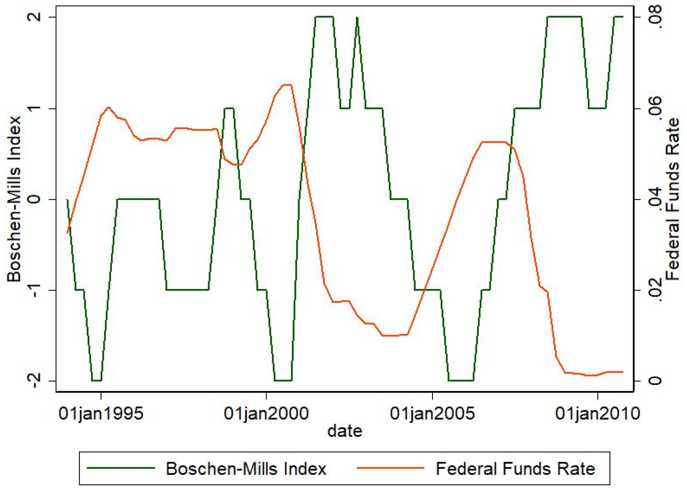
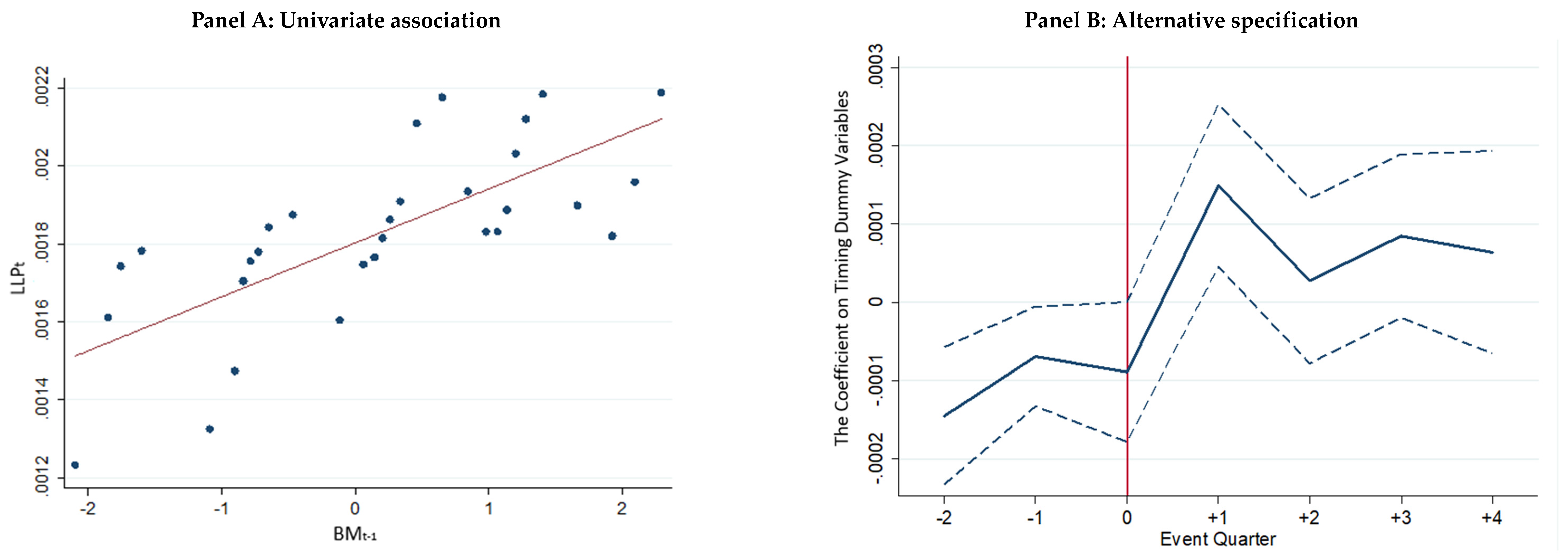
Table 1.
Sample construction.
| Sample Size | |
|---|---|
| Total number of bank-quarters in COMPUSTAT in the period 1995Q1–2010Q416 Less: | 47,919 |
| Drop observations with missing required data in COMPUSTAT | (25,507) |
| Merge with commercial bank call report and bank holding company call report (Y-9C) and drop observations with missing required data | (5853) |
| Merge with CRSP database and drop observations with missing required data | (0) |
| Merge with state and national-level control variables, and exogenous shocks, including Taylor rule residual and drop observations with missing required data17 | (1310) |
| Merge with Adrian and Brunnermeier’s (2016) risk measures and drop observations with missing required data. | (626) |
| The final sample of bank-quarter observations | 14,623 |
Table 1 describes the sample selection process. The sample is collected from the COMPSTAT database and merged with the bank regulatory database (commercial bank call report and bank holding company call report) and CRSP database, including 497 distinct banks and a total number of 14,623 bank-quarter observations in the period 1995Q1–2010Q4.
Table 2.
Summary statistics by policy stances.
| Variable | Non-EMP Periods (BM Index = −2, −1 or 0)18 | EMP Periods19 (BM Index = 1 or 2) | Difference in Means (t-Stat.) | ||||||
|---|---|---|---|---|---|---|---|---|---|
| N | Mean | Std Dev | Median | N | Mean | Std Dev | Median | ||
| LLP | 7930 | 0.001 | 0.001 | 0.001 | 6693 | 0.003 | 0.004 | 0.001 | −45.125 *** |
| CH_NPA | 7930 | 0.000 | 0.003 | 0.000 | 6693 | 0.002 | 0.007 | 0.000 | −24.848 *** |
| SIZE | 7930 | 7.819 | 1.614 | 7.479 | 6693 | 7.824 | 1.530 | 7.498 | −0.587 |
| CH_LOAN | 7930 | 0.034 | 0.057 | 0.024 | 6693 | 0.013 | 0.051 | 0.007 | 23.822 *** |
| CO | 7930 | 0.001 | 0.001 | 0.000 | 6693 | 0.002 | 0.003 | 0.001 | −39.699 *** |
| ALW | 7930 | 0.015 | 0.006 | 0.013 | 6693 | 0.017 | 0.008 | 0.015 | −17.648 *** |
| STD_EBIT | 7930 | 0.001 | 0.002 | 0.001 | 6693 | 0.002 | 0.003 | 0.001 | −20.310 *** |
| EBTP | 7930 | 0.008 | 0.004 | 0.008 | 6693 | 0.006 | 0.005 | 0.006 | 22.563 *** |
| CON | 7930 | 0.010 | 0.019 | 0.004 | 6693 | 0.008 | 0.016 | 0.003 | 8.807 *** |
| COM | 7930 | 0.180 | 0.118 | 0.155 | 6693 | 0.165 | 0.105 | 0.145 | 7.761 *** |
| REAL | 7930 | 0.681 | 0.181 | 0.708 | 6693 | 0.725 | 0.158 | 0.751 | −15.752 *** |
| LOSS | 7930 | 0.023 | 0.150 | 0.000 | 6693 | 0.181 | 0.385 | 0.000 | −33.179 *** |
| TIER1 | 7930 | 0.113 | 0.026 | 0.109 | 6693 | 0.113 | 0.026 | 0.110 | 0.573 |
| BHAR | 7930 | −0.001 | 0.134 | −0.011 | 6693 | −0.004 | 0.225 | −0.008 | 2.918 *** |
| MTB | 7930 | 1.975 | 0.701 | 1.874 | 6693 | 1.391 | 0.806 | 1.300 | 50.662 *** |
| LOGMV | 7930 | −2.517 | 1.812 | −2.891 | 6693 | −2.928 | 1.811 | −3.244 | 14.248 *** |
| CPI | 1604 | 0.007 | 0.007 | 0.007 | 993 | 0.004 | 0.010 | 0.004 | 20.340 *** |
| HOU | 1604 | 0.015 | 0.015 | 0.013 | 993 | 0.002 | 0.019 | 0.005 | 56.819 *** |
| INCOME | 1604 | 0.059 | 0.038 | 0.058 | 993 | 0.026 | 0.051 | 0.032 | 51.926 *** |
| UNEMPLOY | 1604 | 0.005 | 0.168 | −0.023 | 993 | 0.048 | 0.166 | 0.018 | −21.737 *** |
| DEFAULT | 40 | 0.008 | 0.001 | 0.008 | 25 | 0.014 | 0.006 | 0.012 | −80.900 *** |
| GDPGROW | 40 | 0.032 | 0.020 | 0.031 | 25 | 0.013 | 0.032 | 0.021 | 44.537 *** |
Table 2 describes the summary statistics for both the non-EMP periods (i.e., BM Index = −2, −1, or 0) as well as the EMP periods (i.e., BM Index = 1 or 2), including 497 distinct banks and a total of 14,625 bank-quarter observations in the period 1995Q1–2000Q4. All firm-level continuous variables are winsorized at the 1st and 99th percentiles. *** indicates statistical significance at 1%. See Appendix A for variable definitions and measurements.
Table 3.
Baseline regression of discretionary LLP on monetary policy.
| (1) | (2) | (3) | (4) | (5) | (6) | |||||||
| Dependent Variable: | LLPt | LLPt | LLPt | LLPt | LLPt | LLPt | ||||||
| BMt−1 | 0.0092 *** | (5.91) | 0.0117 *** | (3.53) | 0.0108 *** | (3.55) | ||||||
| FFRt−1 | 0.0046 *** | (4.04) | 0.0224 *** | (4.42) | 0.0208 *** | (5.17) | ||||||
| Determinants of nondiscretionary LLP: | ||||||||||||
| CH_NPAt+1 | 0.0204 *** | (4.34) | 0.0191 *** | (4.02) | 0.0190 *** | (3.98) | 0.0223 *** | (4.67) | 0.0192 *** | (4.04) | 0.0191 *** | (3.94) |
| CH_NPAt | 0.0722 *** | (10.09) | 0.0709 *** | (10.32) | 0.0707 *** | (10.18) | 0.0738 *** | (10.27) | 0.0709 *** | (10.27) | 0.0708 *** | (10.15) |
| CH_NPAt−1 | 0.0079 | (1.24) | 0.0059 | (0.91) | 0.0063 | (0.99) | 0.0090 | (1.43) | 0.0062 | (0.97) | 0.0063 | (1.00) |
| CH_NPAt−2 | 0.0123 ** | (2.19) | 0.0101 * | (1.99) | 0.0093 * | (1.71) | 0.0132 ** | (2.31) | 0.0094 * | (1.75) | 0.0089 | (1.60) |
| SIZEt−1 | −0.0000 | (−0.44) | 0.0001 | (1.02) | 0.0001 | (1.04) | −0.0001 | (−1.47) | 0.0001 | (1.15) | 0.0001 | (1.15) |
| CH_LOANt | −0.0007 *** | (−2.83) | −0.0006 ** | (−2.25) | −0.0006 ** | (−2.34) | −0.0008 *** | (−3.46) | −0.0006 ** | (−2.33) | −0.0006 ** | (−2.36) |
| COt | 0.6861 *** | (21.77) | 0.6794 *** | (21.38) | 0.6772 *** | (21.44) | 0.6888 *** | (21.86) | 0.6779 *** | (21.46) | 0.6765 *** | (21.38) |
| ALWt−1 | −0.0493 *** | (−6.20) | −0.0503 *** | (−6.27) | −0.0505 *** | (−6.28) | −0.0514 *** | (−6.18) | −0.0516 *** | (−6.41) | −0.0515 *** | (−6.38) |
| CONt | 0.0032 | (1.56) | 0.0025 | (1.17) | 0.0025 | (1.20) | 0.0032 | (1.54) | 0.0024 | (1.15) | 0.0025 | (1.17) |
| COMt | 0.0021 *** | (3.13) | 0.0021 *** | (3.19) | 0.0021 *** | (3.21) | 0.0022 *** | (3.14) | 0.0022 *** | (3.22) | 0.0022 *** | (3.21) |
| REALt | 0.0010 * | (1.99) | 0.0011 ** | (2.17) | 0.0011 ** | (2.15) | 0.0009 * | (1.69) | 0.0011 ** | (2.16) | 0.0011 ** | (2.14) |
| Determinants of discretionary LLP: | ||||||||||||
| TIER1t−1 | 0.0020 | (1.35) | 0.0021 | (1.64) | 0.0022 * | (1.73) | 0.0015 | (1.02) | 0.0022 * | (1.72) | 0.0023 * | (1.80) |
| EBTPt | 0.0669 *** | (6.71) | 0.0678 *** | (6.93) | 0.0678 *** | (6.91) | 0.0675 *** | (6.61) | 0.0688 *** | (7.04) | 0.0683 *** | (6.97) |
| LOSSt | 0.0029 *** | (14.72) | 0.0029 *** | (14.58) | 0.0029 *** | (14.65) | 0.0029 *** | (14.67) | 0.0029 *** | (14.54) | 0.0028 *** | (14.58) |
| LOGMVt | −0.0001 | (−0.53) | −0.0001 | (−1.45) | −0.0002 | (−1.51) | −0.0000 | (−0.15) | −0.0002 | (−1.64) | −0.0002 * | (−1.67) |
| MTBt | −0.0002 *** | (−4.84) | −0.0001 *** | (−2.86) | −0.0001 *** | (−2.67) | −0.0003 *** | (−5.87) | −0.0001 *** | (−2.83) | −0.0001 ** | (−2.57) |
| STD_Et | 0.0237 | (1.56) | 0.0180 | (1.17) | 0.0169 | (1.08) | 0.0244 | (1.63) | 0.0167 | (1.07) | 0.0160 | (1.02) |
| LLPt−1 | 0.1005 *** | (4.65) | 0.0952 *** | (4.69) | 0.0952 *** | (4.70) | 0.1022 *** | (4.66) | 0.0954 *** | (4.73) | 0.0956 *** | (4.72) |
| State-wide controls: | ||||||||||||
| CPIt | −0.0028 | (−0.80) | −0.0010 | (−0.39) | −0.0030 | (−1.19) | −0.0009 | (−0.40) | ||||
| HOUt | −0.0004 | (−0.25) | 0.0004 | (0.23) | −0.0003 | (−0.25) | −0.0006 | (−0.33) | ||||
| INCOMEt | 0.0003 | (0.75) | 0.0004 | (1.26) | 0.0003 | (0.90) | 0.0003 | (1.10) | ||||
| UNEMPLOYt | −0.0003 ** | (−2.14) | −0.0001 | (−1.14) | −0.0003 *** | (−3.15) | −0.0001 | (−1.20) | ||||
| Nation-wide controls: | ||||||||||||
| BUSCYCLEt | −0.0000 | (−0.24) | 0.0000 | (0.10) | −0.0003 ** | (−2.20) | −0.0003 ** | (−2.39) | ||||
| GDPGROWt | −0.0007 | (−0.72) | −0.0006 | (−0.74) | −0.0003 | (−0.43) | −0.0010 | (−1.21) | ||||
| DEFAULTt | −0.0088 | (−0.72) | 0.0016 | (0.16) | 0.0036 | (0.34) | 0.0050 | (0.55) | ||||
| Lag Macro Controls | No | No | Yes | No | No | Yes | ||||||
| Bank FE | Yes | Yes | Yes | Yes | Yes | Yes | ||||||
| State FE | Yes | Yes | Yes | Yes | Yes | Yes | ||||||
| Year FE | No | Yes | Yes | No | Yes | Yes | ||||||
| Clustered SE | Firm and Quarter | Firm and Quarter | Firm and Quarter | Firm and Quarter | Firm and Quarter | Firm and Quarter | ||||||
| R-squared | 0.80 | 0.81 | 0.81 | 0.80 | 0.81 | 0.81 | ||||||
| N | 14,623 | 14,623 | 14,623 | 14,623 | 14,623 | 14,623 | ||||||
Table 3 reports the results of tests examining the effect of monetary policy on discretionary LLP. The sample consists of bank-quarter observations from 1995 to 2010. All variables are defined in Appendix A. All firm-level continuous variables are winsorized at the 1st and 99th percentiles. All regressions include state, bank, and year-fixed effects. Standard errors are two-way clustered by bank and quarter. t statistics are shown in parentheses. ***, **, and * indicate statistical significance at the 1%, 5%, and 10% levels, respectively. The constant term is not reported.
Table 4.
Expansionary monetary policy and timeliness of LLP.
| Panel A: The effect of EMP on the relation between current LLP and future non-performing loans | ||||||||||||
| (1) | (2) | (3) | (4) | |||||||||
| Dependent Variable: | LLPt | LLPt | LLPt | LLPt | ||||||||
| BMt−1 | 0.0038 *** | (2.59) | 0.0056 * | (1.71) | 0.0048 | (1.60) | 0.0053 * | (1.78) | ||||
| BMt−1*CH_NPA1YR | 0.1449 *** | (2.86) | 0.1097 ** | (2.36) | 0.1023 ** | (2.15) | 0.0866 * | (1.96) | ||||
| BMt−1*CH_NPAt | 1.4046 *** | (3.30) | 1.4077 *** | (2.67) | 1.3862 ** | (2.64) | 1.4129 *** | (2.73) | ||||
| BMt−1*CH_NPAt−1 | 0.5240 | (1.21) | ||||||||||
| BMt−1*CH_NPAt−2 | 0.5174 | (1.31) | ||||||||||
| CH_NPA1YR | 0.0012 ** | (2.17) | 0.0013 ** | (2.41) | 0.0013 ** | (2.48) | 0.0013 ** | (2.49) | ||||
| CH_NPAt | 0.0500 *** | (8.39) | 0.0499 *** | (7.96) | 0.0500 *** | (8.00) | 0.0500 *** | (8.01) | ||||
| CH_NPAt−1 | −0.0032 | (−0.50) | ||||||||||
| CH_NPAt−2 | 0.0015 | (0.27) | ||||||||||
| Bank Controls | Yes | Yes | Yes | Yes | ||||||||
| Macro Controls | Yes | Yes | Yes | Yes | ||||||||
| Lagged Macro Controls | No | No | Yes | No | ||||||||
| Bank FE | Yes | Yes | Yes | Yes | ||||||||
| Year FE | No | Yes | Yes | Yes | ||||||||
| Clustered Standard Error | Bank | Bank, Quarter | Bank, Quarter | Bank, Quarter | ||||||||
| R-squared | 0.80 | 0.80 | 0.80 | 0.80 | ||||||||
| N | 13,987 | 13,987 | 13,987 | 13,987 | ||||||||
| Panel B: The effect of EMP on the relation between current LLP and future net loan charge-offs | ||||||||||||
| (1) | (2) | |||||||||||
| Dependent Variable: | LLPt | LLPt | ||||||||||
| BMt−1 | 0.0094 ** | (2.57) | 0.0045 | (1.43) | ||||||||
| BMt−1*COt+1 | 2.4782 *** | (2.94) | ||||||||||
| COt+1 | 0.0700 *** | (4.66) | ||||||||||
| BMt−1*COt+4 | 1.2594 *** | (3.86) | ||||||||||
| COt+4 | 0.0352 *** | (5.39) | ||||||||||
| BHARt+1 | −0.0003 *** | (−2.95) | ||||||||||
| BHARt+4 | 0.0002 ** | (2.49) | ||||||||||
| Bank-Level Controls | Yes | Yes | ||||||||||
| Macro-Level Controls | Yes | Yes | ||||||||||
| Bank FE | Yes | Yes | ||||||||||
| Year FE | Yes | Yes | ||||||||||
| Clustered Standard Error | Bank, Quarter | Bank, Quarter | ||||||||||
| R-squared | 0.81 | 0.81 | ||||||||||
| N | 14,623 | 13,747 | ||||||||||
Table 4 Panel A reports the effect of monetary policy on the relation between LLP and future, contemporaneous, and past changes in nonperforming loans. Bank and Macros Controls are included. All variables are defined in Appendix A. All firm-level variables are winsorized at the 1st and 99th percentiles. t statistics are shown in parentheses. ***, **, and * indicate statistical significance at the 1%, 5%, and 10% levels, respectively. The constant term is not reported. Table 4, Panel B, reports the correlation between current LLP and future charge-offs in one quarter and one year ahead. Following Hribar et al. (2017), we additionally control for the abnormal return during that period to partial out the unexpected noises in the future charge-off. All variables are defined in Appendix A. All firm-level variables are winsorized at the 1st and 99th percentiles. t statistics are shown in parentheses. ***, **, and * indicate statistical significance at the 1%, 5%, and 10% levels, respectively. The constant term is not reported.
Table 5.
Cross-sectional analyses.
| Panel A: The effect of current bank risk on the relation between LLP and monetary policy | ||||||||||||||||||||||
| (1) | (2) | (3) | ||||||||||||||||||||
| LLPt | LLPt | LLPt | ||||||||||||||||||||
| BMt−1 | 0.0077 ** | (2.31) | 0.0078 ** | (2.29) | 0.0012 | (0.25) | ||||||||||||||||
| BMt−1*STD_Et | 2.3926 *** | (3.56) | ||||||||||||||||||||
| STD_Et | −0.0032 | (−0.23) | ||||||||||||||||||||
| BMt−1*BETAt | 0.0081 *** | (3.52) | ||||||||||||||||||||
| BETAt | 0.0000 | (0.96) | ||||||||||||||||||||
| BMt−1*VaRt | 0.1840 *** | (3.25) | ||||||||||||||||||||
| VaRt | 0.0027 * | (1.92) | ||||||||||||||||||||
| Firm, state, and national controls | Yes | Yes | Yes | |||||||||||||||||||
| Bank, state and year FE | Yes | Yes | Yes | |||||||||||||||||||
| Clustered Standard Error | Firm and Quarter | Firm and Quarter | Firm and Quarter | |||||||||||||||||||
| R-squared | 0.81 | 0.81 | 0.81 | |||||||||||||||||||
| N | 14,625 | 14,625 | 14,625 | |||||||||||||||||||
| Panel B: The moderating effect of historical (past 12 quarters) informativeness of loan loss provisions on the relation between LLP and monetary policy | ||||||||||||||||||||||
| (1) | (2) | |||||||||||||||||||||
| LLPt | LLPt | |||||||||||||||||||||
| BMt−1 | 0.0117 *** | (3.09) | 0.0122 *** | (2.85) | ||||||||||||||||||
| BMt−1*DELRt−1 | 0.0041 *** | (2.71) | ||||||||||||||||||||
| DELRt−1 | 0.0001 *** | (2.99) | ||||||||||||||||||||
| BMt−1*DELR_strictt−1 | 0.0100 *** | (2.88) | ||||||||||||||||||||
| DELR_strictt−1 | 0.0001 *** | (3.55) | ||||||||||||||||||||
| Firm, state, and national controls | Yes | Yes | ||||||||||||||||||||
| Year FE | Yes | Yes | ||||||||||||||||||||
| Clustered Standard Error | Firm and Quarter | Firm and Quarter | ||||||||||||||||||||
| R-squared | 0.80 | 0.78 | ||||||||||||||||||||
| N | 9559 | 4816 | ||||||||||||||||||||
| Panel C: Testing the moderating role of institutional investors | ||||||||||||||||||||||
| (1) LLPt | (2) LLPt | (3) LLPt | (4) LLPt | (5) LLPt | (6) LLPt | |||||||||||||||||
| Monetary Policy (MP) Proxy: | EMPt−1 | EMPt−1 | FFRt−1 | EMPt−1 | FFRt−1 | EMPt−1 | ||||||||||||||||
| MPt−1 | 0.000 | (0.21) | −0.001 ** | (−2.52) | 0.007 | (0.68) | −0.001 ** | (−2.26) | 0.021 ** | (2.01) | −0.001 ** | (−2.46) | ||||||||||
| MPt−1*INSTt (*100) | 0.077 *** | (4.56) | 0.044 *** | (2.86) | 0.013 *** | (3.23) | 0.030 ** | (2.11) | 0.010 ** | (2.47) | −0.001 * | (−1.79) | ||||||||||
| MPt−1*INSTt*FDt (*100) | 0.096 *** | (3.06) | ||||||||||||||||||||
| MPt−1*CH_NPAt+1 | −0.003 | (−0.23) | −0.453 * | (−1.84) | −0.005 | (−0.39) | −0.429 * | (−1.70) | −0.006 | (−0.43) | ||||||||||||
| MPt−1*CH_NPAt | 0.032 ** | (2.35) | 0.132 | (0.43) | 0.030 ** | (2.11) | 0.160 | (0.50) | 0.029 ** | (2.00) | ||||||||||||
| MPt−1*CH_NPAt−1 | 0.008 | (0.88) | −0.107 | (−0.42) | 0.006 | (0.66) | −0.054 | (−0.21) | 0.006 | (0.65) | ||||||||||||
| MPt−1*CH_NPAt−2 | 0.011 | (1.01) | 0.093 | (0.43) | 0.008 | (0.79) | 0.097 | (0.46) | 0.008 | (0.73) | ||||||||||||
| MPt−1*SIZEt−1 | 0.000 ** | (2.32) | −0.001 | (−0.86) | 0.000 ** | (2.50) | −0.001 | (−0.63) | 0.000 *** | (2.69) | ||||||||||||
| MPt−1*CH_LOANt | −0.001 ** | (−2.10) | −0.005 | (−0.30) | −0.001 | (−1.56) | −0.002 | (−0.13) | −0.001 | (−1.66) | ||||||||||||
| MPt−1*COt | 0.255 *** | (5.68) | 4.286 *** | (4.55) | 0.251 *** | (5.48) | 4.172 *** | (4.49) | 0.248 *** | (5.47) | ||||||||||||
| MPt−1*ALWt−1 | −0.020 ** | (−2.47) | −0.649 *** | (−2.68) | −0.018 ** | (−2.23) | −0.591 ** | (−2.57) | −0.016 ** | (−2.05) | ||||||||||||
| MPt−1*CONt | −0.000 | (−0.15) | 0.046 | (1.16) | 0.000 | (0.10) | 0.062 | (1.64) | 0.000 | (0.13) | ||||||||||||
| MPt−1*COMt | 0.001 * | (1.77) | 0.009 | (0.96) | 0.001 | (1.58) | 0.008 | (0.85) | 0.001 * | (1.71) | ||||||||||||
| MPt−1*REALt | 0.001 ** | (2.38) | 0.008 | (1.04) | 0.000 | (1.66) | 0.003 | (0.37) | 0.000 | (1.56) | ||||||||||||
| INSTt | −0.000 | (−0.45) | −0.000 | (−0.51) | 0.001 *** | (2.81) | 0.000 | (0.78) | 0.001 *** | (3.01) | 0.001 ** | (2.21) | ||||||||||
| CH_NPAt+1 | 0.016 *** | (3.01) | 0.018 | (1.65) | 0.009 | (1.20) | 0.019 * | (1.70) | 0.007 | (1.02) | 0.020 * | (1.70) | ||||||||||
| CH_NPAt | 0.075 *** | (9.93) | 0.051 *** | (4.90) | 0.081 *** | (6.90) | 0.052 *** | (4.85) | 0.080 *** | (6.66) | 0.052 *** | (4.80) | ||||||||||
| CH_NPAt−1 | 0.006 | (1.19) | −0.000 | (−0.03) | 0.005 | (0.63) | 0.000 | (0.01) | 0.005 | (0.59) | 0.000 | (0.06) | ||||||||||
| CH_NPAt−2 | 0.012 ** | (2.03) | 0.004 | (0.58) | 0.015 * | (1.75) | 0.004 | (0.58) | 0.013 | (1.54) | 0.004 | (0.53) | ||||||||||
| SIZEt−1 | 0.000 ** | (2.28) | −0.000 | (−0.44) | −0.000 | (−0.74) | 0.000 | (1.60) | 0.000 * | (1.92) | 0.000 | (1.63) | ||||||||||
| CH_LOANt | 0.000 | (−1.35) | 0.000 | (0.73) | −0.001 | (−0.86) | 0.000 | (0.85) | −0.000 | (−0.53) | 0.000 | (0.80) | ||||||||||
| COt | 0.644 *** | (19.65) | 0.453 *** | (11.43) | 0.737 *** | (23.20) | 0.451 *** | (11.23) | 0.728 *** | (23.13) | 0.451 *** | (11.30) | ||||||||||
| ALWt−1 | −0.044 *** | (−5.92) | −0.035 *** | (−5.11) | −0.066 *** | (−6.62) | −0.039 *** | (−5.52) | −0.066 *** | (−7.04) | −0.041 *** | (−5.83) | ||||||||||
| CONt | 0.002 | (0.79) | 0.003 * | (1.71) | 0.004 | (1.41) | 0.002 | (1.00) | 0.004 | (1.21) | 0.002 | (0.91) | ||||||||||
| COMt | 0.002 *** | (2.9) | 0.002 ** | (2.36) | 0.002 *** | (2.78) | 0.002 ** | (2.51) | 0.002 *** | (2.82) | 0.002 ** | (2.45) | ||||||||||
| REALt | 0.001 | (1.35) | 0.000 | (0.22) | 0.000 | (0.78) | 0.000 | (0.87) | 0.001 | (0.99) | 0.000 | (0.82) | ||||||||||
| Other Bank-Level Controls | Yes | Yes | Yes | Yes | Yes | Yes | ||||||||||||||||
| Macro Controls | Yes | Yes | Yes | Yes | Yes | Yes | ||||||||||||||||
| Bank FE | Yes | Yes | Yes | Yes | Yes | Yes | ||||||||||||||||
| Year FE | Yes | No | No | Yes | Yes | Yes | ||||||||||||||||
| SE clustered in | Bank, Quarter | Bank, Quarter | Bank, Quarter | Bank, Quarter | Bank, Quarter | Bank, Quarter | ||||||||||||||||
| R-squared | 0.79 | 0.81 | 0.80 | 0.81 | 0.81 | 0.81 | ||||||||||||||||
| N | 12,281 | 12,281 | 12,281 | 12,281 | 12,281 | 12,281 | ||||||||||||||||
Table 5 Panel A reports the moderating effect of bank risk on the relation between LLP and monetary policy. The risks are measured by either historical book volatility (STD_E) or market-based measures of risks (VaR or BETA). Our sample consists of bank-quarter observations from 1995 to 2010. All variables are defined in Appendix A. All firm-level continuous variables are winsorized at the 1st and 99th percentiles. t statistics are shown in parentheses. ***, **, and * indicate statistical significance at the 1%, 5%, and 10% levels, respectively. The constant term is not reported. Panel B reports the moderating effect of the historical informativeness of loan loss information. While DELRt−1 represents those banks whose estimated future loan losses are less informative and accurate, DELR_strictt−1 proxied for more egregious banks in estimating future loan losses. Our sample consists of bank-quarter observations from 1995 to 2010. All firm-level continuous variables are winsorized at the 1st and 99 percentiles. All variables are defined in Appendix A. t statistics are shown in parentheses. ***, **, and * indicate statistical significance at the 1%, 5%, and 10% levels, respectively. The constant term is not reported. Table 5 Panel C reports the moderating effect of institutional investors on the relation between LLP and monetary policy. The FD dummy variable equals 1 for all the bank-quarter observations subsequent to October 2000, when Reg FD became effective, and 0 otherwise. Our sample consists of bank-quarter observations from 1995 to 2010. The dependent variables are EMPt−1 (a dummy variable that equals 1 when monetary policy is expansionary) and FFRt−1. Column 1 shows the results without allowing the mapping of LLP to its determinants to vary with EMP. Columns 2 and 3 allow the mapping of LLP to its determinants to vary with EMP but do not incorporate year-fixed effects. Columns 4 and 5 allow the mapping of LLP to its determinants to vary with EMP, together with all control variables, bank fixed effects, and year fixed effects. Column 6 repeats the regression in Model 4 but adds the interaction of FDt. Standard errors are clusters at Bank and Quarter. All firm-level continuous variables are winsorized at the 1st and 99th percentiles. All variables are defined in Appendix A. t statistics are shown in parentheses. ***, **, and * indicate statistical significance at the 1%, 5%, and 10% levels, respectively. The constant term is not reported.
Table 6.
The moderating role of bank regulation.
| Panel A: Testing the effect of the FDICIA internal control rule on the relation between EMP and DLLP | |||||||||||||||
| (1) Nearest-Neighbor Matching | (2) Nearest-Neighbor Matching | (3) Epanechnikov Kernel | (4) Epanechnikov Kernel | (5) Nearest-Neighbor Matching | (6) Linear Regression | ||||||||||
| Subsample condition: | ABOVE500 = 1 | ABOVE500 = 0 | ABOVE500 = 1 | ABOVE500 = 0 | EMPt−1 = 1 | Full Sample | |||||||||
| Outcome Var. | DLLP | DLLP | DLLP | DLLP | DLLP | LLP | |||||||||
| ABOVE500 | 0.0305 *** (t = 2.62) | ||||||||||||||
| EMPt−1 | 0.029 ** (t = 2.37) | 0.0099 (t = 0.67) | 0.28 *** (t = 7.30) | 0.0123 (t = 1.56) | |||||||||||
| EMPt−1 × ABOVE500 | 0.0148 ** (t = 2.08) | ||||||||||||||
| Bank, State, and National Control Variables | Yes | Yes | Yes | Yes | Yes | Yes | |||||||||
| Bank and Year FE | No | No | No | No | No | Yes | |||||||||
| Standard Error | AI (2006) | AI (2006) | Bootstrapped | Bootstrapped | AI (2006) | Bank, Quarter | |||||||||
| R-squared | 0.3268 | 0.1781 | 0.3268 | 0.1781 | 0.1467 | 0.7648 | |||||||||
| N | 13,105 | 1503 | 13,105 | 1503 | 6683 | 14,602 | |||||||||
| Panel B: Testing the effect of state regulatory scrutiny on the relation between EMP and DLLP | |||||||||||||||
| (1) | (2) | (3) | (4) | ||||||||||||
| LLPt | LLPt | LLPt | LLPt | ||||||||||||
| (Strict = 1) | (Strict = 0) | (Strict = 1) | (Strict = 0) | ||||||||||||
| BMt−1 | 0.0040 *** | (2.75) | 0.0032 ** | (2.29) | |||||||||||
| BMt−1*StateCharter | 0.0002 | (0.20) | −0.0027 ** | (−2.41) | |||||||||||
| FFRt−1 | 0.0139 *** | (7.99) | 0.0102 *** | (5.85) | |||||||||||
| FFRt−1*StateCharter | 0.0003 | (0.45) | −0.0023 *** | (−3.43) | |||||||||||
| StateCharter | 0.0000 *** | (2.69) | −0.0000 | (−0.15) | 0.0000 * | (1.84) | −0.0001 *** | (−2.73) | |||||||
| Comparison: | BMt−1*StateCharter | FFRt−1*StateCharter | |||||||||||||
| Chi square statistics | 3.39 | 7.47 | |||||||||||||
| p-value | 0.0657 | 0.0063 | |||||||||||||
| Bank, State, and National Control Variables | Yes | Yes | Yes | Yes | |||||||||||
| State and Year FE | Yes | Yes | Yes | Yes | |||||||||||
| R-squared | 0.69 | 0.73 | 0.69 | 0.73 | |||||||||||
| N | 150,283 | 122,346 | 154,563 | 125,285 | |||||||||||
Table 6, Panel A, reports results using various setups of propensity score matching and a linear regression with fixed effects. ABOVE500 is the status of receiving “treatment” from stricter regulation according to the FDICIA rule; it equals one if the bank’s total assets are above USD 500 million. In Columns 1, 2, and 5, treated and control groups are 1-on-4 matched based on lagged real GDP growth, CPI growth, housing price growth, income growth, unemployment growth, and firm-level variables. Columns 3 and 4 use Epanechnikov kernel matching. We impose common support by dropping 10% of the treatment observations at which the p-score density of the control observations is the lowest. We use a caliper of 0.05 (which is 0.25 * the standard deviation of propensity scores) for the nearest-neighbor matchings. Column 5 restricts the subsample to banks under EMP and tests the treatment effect of receiving stricter internal control regulations. Column 6 is a linear regression model with bank and year-quarter fixed effects. All firm-level variables are winsorized at 1% and 99%. ***, **, and * indicate statistical significance at the 1%, 5%, and 10% levels, respectively. All coefficients are multiplied by 100. Table 6, Panel B, reports the results of testing the joint effects of state regulatory strictness and bank charter type (i.e., state vs. national) on the relation between EMP and DLLP. Data from bank call reports are used in these tests to include all commercial banks. StateCharter equals 1 if the bank is state-chartered, and 0 if the bank is a national bank. Strict equals 1 if a state’s regulatory index falls into the highest tercile of the state regulatory index constructed by Agarwal et al. (2014) and 0 if a state’s regulatory index falls into the lowest tercile. The reported Chi square statistics test the significance of differences between the coefficients (BMt−1*StateCharter) in Model (1) and Model (2) and the coefficients (FFRt−1*StateCharter) in Model (3) and Model (4). All firm-level variables are winsorized at 1% and 99%. ***, **, and * indicate statistical significance at the 1%, 5%, and 10% levels, respectively.
Table 7.
Path analysis of the direct and indirect effects of monetary policy.
| Coefficients | t-Stat. | |
|---|---|---|
| Direct Path | ||
| p (TRRt−1, DLLPt) | 0.008 *** | (8.17) |
| Indirect Path | ||
| p (TRRt−1, VaRt) | 0.811 *** | (32.82) |
| p (VaRt, DLLPt) | 0.007 *** | (7.02) |
| Total magnitude of the indirect effect | 0.006 *** | (6.97) |
| Percentage of the direct effect to the total effect | 57.14% | |
| Percentage of the indirect effect to the total effect | 42.85% | |
| Nation-wide and state-wide controls | Yes | |
| Firm-level controls | Yes | |
| N | 14,619 |
Table 7 reports result from a path analysis that examines the direct effect and the indirect effect through increases in bank riskiness. A recursive path model with observable variables is used. ***, **, and * indicate statistical significance at the 1%, 5%, and 10% levels, respectively. The standard error is heteroskedasticity-robust. All firm-level continuous variables are winsorized at the 1st and 99th percentiles. The constant term is not reported.
Table 8.
The relation between monetary policy and DLLP: instrumental variable (2SLS) estimation.
| (1) | (2) | (3) | (4) | |||||
| 1st Stage | 2nd Stage | 1st Stage | 2nd Stage | |||||
| Dependent Variable: | BMt−1 | LLPt | FFRt−1 | LLPt | ||||
| Pred_BMt−1 | 0.0358 *** | (3.08) | ||||||
| Pred_FFRt−1 | 0.0450 *** | (3.09) | ||||||
| SURPRISEt−2 | 0.045 *** | (22.81) | 0.035 *** | (28.05) | ||||
| CH_NPAt+1 | −0.011 | (−1.21) | 0.020 *** | (8.30) | −0.008 *** | (−1.33) | 0.020 *** | (8.31) |
| CH_NPAt | −0.009 | (−0.94) | 0.074 *** | (28.85) | −0.01 *** | (−1.58) | 0.075 *** | (28.97) |
| CH_NPAt−1 | −0.024 ** | (−2.21) | 0.008 *** | (2.70) | −0.015 *** | (−2.16) | 0.008 *** | (2.65) |
| CH_NPAt−2 | −0.016 | (−1.44) | 0.011 *** | (3.85) | 0.009 *** | (1.18) | 0.011 *** | (3.54) |
| SIZEt−1 | −0.001 *** | (−4.85) | 0.000 ** | (2.25) | −0.002 ** | (−9.12) | 0.000 ** | (2.53) |
| CH_LOANt | −0.001 | (−1.13) | −0.001 ** | (−2.20) | 0.000 ** | (−0.36) | −0.001 ** | (−2.33) |
| COt | 0.023 | (0.78) | 0.695 *** | (89.62) | 0.062 *** | (3.29) | 0.693 *** | (89.01) |
| ALWt−1 | 0.032 ** | (2.45) | −0.055 *** | (−15.70) | 0.056 *** | (6.59) | −0.056 *** | (−15.79) |
| CONt | 0.005 | (0.92) | 0.003 * | (1.81) | 0.002 * | (0.6) | 0.003 * | (1.88) |
| COMt | −0.001 | (−0.84) | 0.002 *** | (5.70) | −0.001 *** | (−0.55) | 0.002 *** | (5.67) |
| REALt | 0.000 | (−0.17) | 0.001 *** | (4.27) | 0.000 *** | (0.24) | 0.001 *** | (4.24) |
| TIER1t−1 | −0.003 | (−1.09) | 0.003 *** | (3.32) | −0.007 *** | (−3.65) | 0.003 *** | (3.56) |
| EBTPt | 0.033 * | (1.94) | 0.065 *** | (14.06) | −0.003 *** | (−0.25) | 0.066 *** | (14.45) |
| LOSSt | 0.000 | (0.44) | 0.003 *** | (46.34) | 0.000 *** | (3.18) | 0.003 *** | (45.83) |
| LOGMVt | 0.001 *** | (4.69) | −0.000 *** | (−3.71) | 0.002 *** | (11.56) | −0.000 *** | (−4.11) |
| MTBt | −0.001 *** | (−5.98) | −0.000 *** | (−3.58) | 0.000 *** | (−5.08) | −0.000 *** | (−3.89) |
| STD_Et | 0.016 | (0.62) | 0.017 ** | (2.47) | 0.057 ** | (3.43) | 0.015 ** | (2.16) |
| LLPt−1 | −0.032 | (−1.22) | 0.087 *** | (12.53) | −0.035 *** | (−2.04) | 0.088 *** | (12.62) |
| CPIt | −0.23 *** | (−30.29) | 0.006 | (1.63) | −0.114 | (−23.16) | 0.003 | (0.97) |
| HOUt | 0.046 *** | (9.01) | −0.001 | (−0.35) | 0.071 | (21.27) | −0.002 | (−1.24) |
| INCOMEt | −0.024 *** | (−19.29) | 0.001 ** | (2.47) | −0.009 * | (−11.68) | 0.001 * | (1.83) |
| UNEMPLOYt | −0.003 *** | (−6.28) | −0.000 | (−0.42) | −0.001 | (−4.32) | −0.000 | (−0.80) |
| BUSCYCLEt | 0.011 *** | (35.95) | −0.000 * | (−1.87) | 0.019 ** | (95.61) | −0.001 *** | (−2.58) |
| GDPGROWt | −0.009 ** | (−2.57) | −0.001 | (−0.77) | 0.010 | (4.13) | −0.001 | (−1.52) |
| DEFAULTt | −1.265 *** | (−38.2) | 0.034 ** | (2.03) | −0.803 * | (−37.51) | 0.025 * | (1.74) |
| Lagged Macro Controls | Yes | Yes | Yes | Yes | ||||
| Bank FE | Yes | Yes | Yes | Yes | ||||
| Year FE | Yes | Yes | Yes | Yes | ||||
| Cragg–Donald F-stat | 520.43 | 786.93 | ||||||
| R-squared | 0.06 | 0.77 | 0.06 | 0.77 | ||||
| N | 13,122 | 13,122 | 13,122 | 13,122 | ||||
Table 8 reports the regression results of the relation between monetary policy and DLLP, based on an instrumental variable (2SLS) approach. SURPRISE is the negative of the three-month-ahead Fed funds futures surprises reported in Gertler and Karadi (2015). Following Kuttner (2001) and Gorodnichenko and Weber (2016), we use lagged SURPRISE at t−2 as the instrumental variable for the actual monetary policy at t−1. In Column 1, we report the results of the first-stage regression, where we regress BMt−1 on SURPRISEt−2 as the instrument and other control variables in the main regression with bank and year fixed effects. In Column 2, we report the second-stage results using the predicted value of BMt−1 from the first stage. In Columns 3 and 4, we repeat the 2SLS regressions but using FFRt−1 as the proxy for monetary policy. The detailed definitions of all variables are provided in Appendix A. The t-statistics reported in parentheses are based on standard errors clustered by banks. ***, **, and * indicate significance at the 1%, 5%, and 10% levels (two-tailed), respectively.
Table 9.
The consequences of conservative loan loss provisioning.
| (1) | (2) | (3) | (4) | (5) | (6) | |
| Dependent Var: | CH_VaRt+4/t | CH_VaRt+4/t | CH_VaRt+4/t | CH_VaRt+4/t | ΔσROAt | ΔZScoret |
| Proxy for DLLP: | n/a | HIGHDLLP | POSDLLP | DLLP | DLLP | DLLP |
| BMt−1 | 0.454 *** | 0.524 *** | 0.531 *** | 0.460 *** | 0.008 | 0.004 |
| (13.08) | (12.32) | (12.63) | (13.17) | (1.45) | (0.22) | |
| DLLP_PROXY*BMt−1 | −0.132 *** | −0.149 *** | −70.43 *** | −16.141 *** | −28.248 ** | |
| (−2.97) | (−3.39) | (−3.17) | (−3.67) | (−2.52) | ||
| DLLP_PROXY | −0.001 | −0.001 * | −0.317 | −0.225 *** | −0.465 *** | |
| (−1.38) | (−1.76) | (−0.99) | (−3.19) | (−3.31) | ||
| CONt−1 | −0.007 | −0.007 | −0.007 | −0.006 | −0.010 | 0.009 |
| (−0.42) | (−0.39) | (−0.42) | (−0.36) | (−1.26) | (0.48) | |
| COMt−1 | −0.007 | −0.008 | −0.008 | −0.007 | 0.013 * | 0.017 * |
| (−0.79) | (−0.84) | (−0.86) | (−0.73) | (1.94) | (1.65) | |
| REALt−1 | 0.007 | 0.007 | 0.007 | 0.008 | 0.008 * | 0.003 |
| (1.00) | (0.96) | (0.93) | (1.06) | (1.90) | (0.41) | |
| ROAt−1 | 0.363 *** | 0.367 *** | 0.368 *** | 0.387 *** | 0.167 *** | 0.264 *** |
| (3.95) | (3.98) | (3.98) | (4.03) | (6.29) | (5.18) | |
| DEPOSITt−1 | 0.002 | 0.002 | 0.002 | 0.002 | −0.002 ** | −0.010 *** |
| (0.56) | (0.54) | (0.54) | (0.52) | (−2.47) | (−3.61) | |
| SIZEt−1 | −0.002 | −0.002 | −0.002 | −0.002 | 0.000 | 0.003 |
| (−1.27) | (−1.34) | (−1.34) | (−1.31) | (0.31) | (1.37) | |
| CH_LOANt | 0.010 * | 0.010 * | 0.010 * | 0.009 | −0.003 * | −0.007 ** |
| (1.69) | (1.68) | (1.68) | (1.63) | (−1.94) | (−2.30) | |
| EBTPt | 0.658 *** | 0.650 *** | 0.647 *** | 0.627 *** | 0.314 *** | 0.684 *** |
| (4.36) | (4.33) | (4.31) | (4.18) | (8.33) | (7.99) | |
| TIER1t−1 | −0.066 *** | −0.065 *** | −0.065 *** | −0.063 *** | −0.026 *** | −0.055 ** |
| (−3.03) | (−3.00) | (−2.99) | (−2.88) | (−3.20) | (−2.45) | |
| BETAt | 0.000 | 0.000 | 0.000 | 0.000 | 0.000 | −0.000 |
| (0.24) | (0.24) | (0.25) | (0.34) | (0.05) | (−0.62) | |
| ILLIQUIDITYt | −0.005 *** | −0.005 *** | −0.005 *** | −0.005 *** | −0.000 ** | −0.000 |
| (−10.61) | (−10.60) | (−10.61) | (−10.64) | (−2.19) | (−0.02) | |
| Bank FE | Yes | Yes | Yes | Yes | Yes | Yes |
| Year FE | Yes | Yes | Yes | Yes | Yes | Yes |
| Clustered SE | Bank | Bank | Bank | Bank | Bank | Bank |
| R-squared | 0.31 | 0.31 | 0.31 | 0.31 | 0.28 | 0.35 |
| N | 11,672.00 | 11,672.00 | 11,672.00 | 11,663.00 | 12,575.00 | 7576.00 |
Table 9 reports the effect of DLLP on the relationship between expansionary monetary policy and future changes in bank risk and the effect of long-term commitment on LLP timeliness. In column 1, CH_VaRt+4/t is regressed on BMt−1 without any interactions. In columns 2, 3, and 4, CH_VaRt+4/t is regressed on the interaction between BMt−1 and different proxies of DLLP to examine the effect of DLLP on the relation between monetary policy and future changes in bank risk. In columns 5 and 6, ΔσROA and ΔZScoret are used as dependent variables. All variables are defined in Appendix A. All firm-level continuous variables are winsorized at the 1st and 99th percentiles. t statistics are shown in parentheses. ***, **, and * indicate statistical significance at the 1%, 5%, and 10% levels, respectively. The constant term is not reported.
Table 10.
The consequences of a long-term commitment to timely LLP versus a temporary change to timely LLP.
Table 10.
The consequences of a long-term commitment to timely LLP versus a temporary change to timely LLP.
| (1) | (2) | (3) | (4) | (5) | (6) | |||||||
| Dependent Variable: | CH_VaRt+4/t | CH_VaRt+4/t | CH_VaRt+4/t | CH_VaRt+4/t | CH_VaRt+4/t | CH_VaRt+4/t | ||||||
| Proxy for MPt−1 | BMt−1 | EMPt−1 | TRRt−1 | BMt−1 | EMPt−1 | TRRt−1 | ||||||
| Sub-Sample Condition | TIMELYt+11/t = 1 | TIMELYt+11/t = 1 | TIMELYt+11/t = 1 | TIMELYt+11/t = 1 | TIMELYt+11/t = 1 | TIMELYt+11/t = 1 | ||||||
| EMPt−1 | 0.632 *** | (9.96) | 0.036 *** | (13.83) | −0.111 *** | (−4.50) | 0.611 *** | (9.30) | 0.036 *** | (12.63) | −0.121 *** | (−5.06) |
| DLLPt | 0.008 | (1.04) | −0.008 | (−1.26) | 0.012 | (1.29) | 0.007 | (1.03) | −0.003 | (−0.59) | 0.016 | (1.62) |
| EMPt−1*DLLPt | 1.056 | (1.55) | 0.019 | (1.12) | −0.133 | (−0.54) | 0.691 | (1.52) | 0.008 | (0.59) | −0.159 | (−0.63) |
| TIMELYt+23/t | −0.001 | (−1.31) | −0.002 * | (−1.78) | 0.003 *** | (2.99) | ||||||
| TIMELYt+23/t*EMPt−1 | −0.220 *** | (−3.41) | 0.002 | (1.11) | −0.305 *** | (−8.88) | ||||||
| TIMELYt+23/t*DLLPt | −0.014 | (−1.44) | 0.005 | (0.60) | −0.001 | (−0.09) | ||||||
| TIMELYt+23/t*EMPt−1*DLLPt | −2.552 *** | (−3.02) | −0.046 ** | (−2.22) | −0.959 ** | (−2.33) | ||||||
| TIMELYt+35/t | −0.003 * | (−1.81) | −0.003 ** | (−2.06) | 0.002 | (1.60) | ||||||
| TIMELYt+35/t*EMPt−1 | −0.187 *** | (−2.85) | 0.002 | (0.84) | −0.294 *** | (−8.18) | ||||||
| TIMELYt+35/t*DLLPt | −0.015 | (−1.59) | −0.002 | (−0.26) | −0.007 | (−0.62) | ||||||
| TIMELYt+35/t*EMPt−1*DLLPt | −2.255 *** | (−3.27) | −0.034 * | (−1.77) | −0.907 ** | (−2.23) | ||||||
| CONt−1 | 0.009 | (0.30) | −0.007 | (−0.29) | 0.009 | (0.27) | 0.002 | (0.07) | −0.015 | (−0.62) | 0.010 | (0.29) |
| COMt−1 | −0.006 | (−0.37) | −0.004 | (−0.27) | −0.004 | (−0.31) | −0.006 | (−0.37) | −0.005 | (−0.31) | −0.003 | (−0.18) |
| REALt−1 | 0.005 | (0.41) | 0.001 | (0.07) | 0.004 | (0.40) | 0.004 | (0.29) | −0.001 | (−0.05) | 0.007 | (0.58) |
| ROAt−1 | 0.401 *** | (3.54) | 0.408 *** | (3.83) | 0.332 *** | (2.90) | 0.401 *** | (3.54) | 0.413 *** | (3.89) | 0.327 *** | (2.86) |
| DEPOSITt−1 | 0.001 | (0.14) | −0.000 | (−0.02) | −0.000 | (−0.05) | 0.001 | (0.17) | −0.000 | (−0.03) | −0.001 | (−0.14) |
| SIZEt−1 | −0.002 | (−0.97) | −0.003 | (−1.19) | −0.000 | (−0.09) | −0.003 | (−1.07) | −0.003 | (−1.34) | 0.000 | (0.00) |
| CH_LOANt | 0.008 | (1.01) | 0.008 | (1.04) | 0.009 | (1.14) | 0.008 | (1.05) | 0.008 | (1.00) | 0.009 | (1.10) |
| EBTPt | 0.846 *** | (3.31) | 0.937 *** | (3.80) | 0.737 *** | (3.18) | 0.839 *** | (3.29) | 0.935 *** | (3.80) | 0.733 *** | (3.17) |
| TIER1t−1 | −0.111 *** | (−3.44) | −0.118 *** | (−3.81) | −0.111 *** | (−3.51) | −0.106 *** | (−3.30) | −0.115 *** | (−3.74) | −0.110 *** | (−3.51) |
| BETAt | 0.003 *** | (2.88) | 0.002 ** | (2.27) | 0.003 *** | (3.20) | 0.003 *** | (2.99) | 0.002 ** | (2.33) | 0.003 *** | (3.26) |
| ILLIQUIDITY | −0.004 *** | (−5.27) | −0.005 *** | (−5.68) | −0.003 *** | (−4.52) | −0.004 *** | (−5.25) | −0.005 *** | (−5.66) | −0.003 *** | (−4.53) |
| MTBt | 0.001 | (0.74) | 0.001 | (0.78) | −0.000 | (−0.03) | 0.001 | (0.73) | 0.001 | (0.73) | 0.000 | (0.04) |
| Constant | 0.015 | (0.65) | 0.009 | (0.40) | 0.003 | (0.15) | 0.018 | (0.78) | 0.013 | (0.59) | 0.001 | (0.04) |
| Bank FE | Yes | Yes | Yes | Yes | Yes | Yes | ||||||
| Year FE | Yes | Yes | Yes | Yes | Yes | Yes | ||||||
| Clustered SE | Bank | Bank | Bank | Bank | Bank | Bank | ||||||
| R-squared | 0.39 | 0.44 | 0.42 | 0.39 | 0.44 | 0.42 | ||||||
| N | 5085 | 5085 | 5085 | 5085 | 5085 | 5085 | ||||||
Table 10 reports the moderating effect of long-term commitment to timely LLP on the risk-disciplinary effect of DLLP when exposed to expansionary monetary policy. DLLPt is scaled by 100 for display purposes. All variables are defined in Appendix A of the paper. t statistics are shown in parentheses. ***, **, and * indicate statistical significance at the 1%, 5%, and 10% levels, respectively. The constant terms are not reported.
Table 11.
Sensitivity Tests.
| (1) | (2) | (3) | (4) | (5) | (6) | |
| States NOT highly correlated with U.S. economy | States highly correlated with U.S. economy | Crisis period | Non-crisis period | Periods with more bank failures | Periods with less bank failures | |
| BMt−1 | 0.0150 *** | 0.0126 *** | 0.0415 *** | 0.0121 *** | 0.0680 ** | 0.0104 *** |
| (3.55) | (3.87) | (4.46) | (3.93) | (2.81) | (4.46) | |
| Firm Level Control | Yes | Yes | Yes | Yes | Yes | Yes |
| State Level Control | Yes | Yes | Yes | Yes | Yes | Yes |
| National Level Control | Yes | Yes | Yes | Yes | Yes | Yes |
| Bank FE | Yes | Yes | Yes | Yes | Yes | Yes |
| State FE | Yes | Yes | Yes | Yes | Yes | Yes |
| Year FE | No | No | No | No | No | No |
| Clustered Standard Error | Bank and Quarter | Bank and Quarter | Bank and Quarter | Bank and Quarter | Bank and Quarter | Bank and Quarter |
| R-squared | 0.69 | 0.67 | 0.74 | 0.68 | 0.68 | 0.52 |
| N | 9150 | 5331 | 2084 | 12,372 | 3444 | 11,030 |
Table 11 reports the result of the sensitivity test. Our sample consists of bank-quarter observations from 1995 to 2010. All variables are defined in Appendix A. All firm-level continuous variables are winsorized at the 1st and 99th percentiles. All regressions include state, bank, and year-fixed effects. Standard errors are two-way clustered by bank and quarter. T statistics are shown in parentheses. ***, **, and * indicate statistical significance at the 1%, 5%, and 10% levels, respectively. The constant term is not reported.
Table 12.
Nonparametric and nonlinear tests, sample composite tests, and heterogeneous effects.
| Panel A: Nonparametric and nonlinear tests | |||||||
| (1) Nearest-Neighbor Matching (N = 4) | (2) Epanechnikov Kernel | (3) Heckman Treatment Effect Model | |||||
| EMPt−1 | 0.0151 *** (3.39) | 0.0198 *** (4.00) | 0.0308 *** (7.68) | ||||
| Bank FE | No | No | No | ||||
| State FE | No | No | No | ||||
| Year FE | No | No | No | ||||
| Rho | −0.0332 | ||||||
| Standard Error | AI (2006) | Bootstrapped | Bootstrapped | ||||
| R-squared | 0.2729 | 0.719 | 0.719 | ||||
| N | 14,608 | 14,608 | 14,608 | ||||
| Panel B: Sample composite tests and heterogeneous effects | |||||||
| (1) | (2) | (3) | (4) | ||||
| Weighted by 1/Frequency of Year | Weighted by 1/Frequency of Bank | Allow macroeconomic variables to have heterogeneous effects | Allow firm characters to have heterogeneous effects | ||||
| BMt−1 | 0.0137 *** (3.21) | 0.0226 *** (4.20) | 0.0313 *** (3.87) | 0.0346 *** (2.90) | |||
| Bank FE | Yes | Yes | Yes | Yes | |||
| State FE | Yes | Yes | Yes | Yes | |||
| Year FE | Yes | Yes | Yes | Yes | |||
| Standard Error | Bank and Quarter | Bank and Quarter | Bank and Quarter | Bank and Quarter | |||
| R-squared | 0.719 | 0.719 | 0.719 | 0.719 | |||
| N | 14,623 | 14,623 | 14,623 | 14,623 | |||
Panel A of Table 12 reports results using nonparametric methods, nonlinear methods, and weighted least squares regression. EMPt−1 is the status of receiving “treatment” for monetary expansion. It equals 1 when the BM index in the t−1 quarter equals 1 or 2, and 0 otherwise. In the propensity score matching, the dependent variable is unexplained discretionary loan loss provision. The treated and control groups are one-on-one matched based on lagged real GDP growth, CPI growth, housing price growth, income growth, and unemployment growth, as well as firm-level variables such as earnings, Tier-1 capital, and market-to-book ratios. In Column 1, we implement nearest-neighbor matching for the observations, with EMPt−1 equal to 1. The standard errors are Abadie and Imbens (2012) robust. In Column 2, we implement the Epanechnikov kernel matching for all the observations in our sample. The standard errors are bootstrapped. Propensity scores are calculated using the logit function. We impose common support by dropping 10 percent of the treatment observations at which the p-score density of the control observations is the lowest. We use a caliper of 0.25 for both matches. In the Hackman treatment effect (Column 3), the first-stage treatment variable is estimated based on two measures of exogenous variations of monetary policy along with all the macroeconomic variables. In both stages, the standard error is bootstrapped. Panel B of Table 12 reports results using nonparametric methods, nonlinear methods, and weighted least squares regression. In Columns 1 and 2, we implement the weighted least square. The weighting is the inverse of year frequency and that of bank frequency. In Columns 3 and 4, we allow macroeconomic variables and firm characteristics that determine accounting discretions to have heterogeneous effects on LLP in response to different policy stances. ***, **, and * indicate statistical significance at the 1%, 5%, and 10% levels, respectively. The constant term is not reported. All firm-level continuous variables are winsorized at the 1st and 99th percentiles.
Table 13.
Additional robustness tests.
| Panel A: Results of baseline regression using exogenous variations in monetary policy | ||||||||
| (1) | (2) | |||||||
| LLPt | LLPt | |||||||
| TRRt−1 | 0.0042 *** | (3.02) | ||||||
| RRSt−1 | 0.0003 *** | (4.95) | ||||||
| Firm and Macro controls | Yes | Yes | ||||||
| Bank, State, and Year FE | Yes | Yes | ||||||
| Clustered Standard Error | Firm and Quarter | Firm and Quarter | ||||||
| R-squared | 0.81 | 0.65 | ||||||
| N | 14,623 | 11,071 | ||||||
| Panel B: Timing of response to monetary policy change | ||||||||
| (1) Placebo Test | (2) Placebo Test | (3) Cumulative effect | (4) Cumulative effect | |||||
| TRRt+1 | −0.0017 | |||||||
| (−1.08) | ||||||||
| RRSt+1 | 0.0001 * | |||||||
| (1.74) | ||||||||
| 0.0193 *** (16.74) | ||||||||
| 0.0189 *** (15.16) | ||||||||
| Lagged and Current Macroeconomic | Yes | Yes | Yes | Yes | ||||
| Bank, State, and year FE | Yes | No | Yes | Yes | ||||
| Clustered Standard Error | Bank and Quarter | Bank and Quarter | Bank and Quarter | Bank and Quarter | ||||
| R-squared | 0.81 | 0.64 | 0.81 | 0.81 | ||||
| N | 14,623 | 11,071 | 14,623 | 14,623 | ||||
Table 13, Panel A, reports the results of tests in which we follow Dell’Ariccia et al. (2017) and replace the interest rate with two measures of exogenous monetary policy. Romer and Romer’s (2004) exogenous shock is available until 2007. The rest of the sample consists of bank-quarter observations from 1995 to 2010. All variables are defined in Appendix A. All firm-level continuous variables are winsorized at the 1st and 99th percentiles. All regressions include state, bank, and year-fixed effects. Standard errors are two-way clustered by bank and quarter. t statistics are shown in parentheses. ***, **, and * indicate statistical significance at the 1%, 5%, and 10% levels, respectively. The constant term is not reported. Table 13, Panel B, shows the results of testing the timing of the response to monetary policy change. In Columns 1 and 2, we perform placebo tests to check the robustness of our exogenous monetary variables. In Columns 3 and 4, we consider the cumulative effect of monetary policy and use the current term along with five lagged terms. The sums of coefficients are shown for the policy variables. F-test statistics are shown in the parentheses. ***, **, and * indicate statistical significance at the 1%, 5%, and 10% levels, respectively. All firm-level continuous variables are winsorized at the 1st and 99th percentiles. The constant term is not reported.
Disclaimer/Publisher’s Note: The statements, opinions and data contained in all publications are solely those of the individual author(s) and contributor(s) and not of MDPI and/or the editor(s). MDPI and/or the editor(s) disclaim responsibility for any injury to people or property resulting from any ideas, methods, instructions or products referred to in the content. |
© 2023 by the authors. Licensee MDPI, Basel, Switzerland. This article is an open access article distributed under the terms and conditions of the Creative Commons Attribution (CC BY) license (https://creativecommons.org/licenses/by/4.0/).
Share and Cite
MDPI and ACS Style
Guo, M.; Jia, X.; Jin, J.Y.; Kanagaretnam, K.; Lobo, G.J. Expansionary Monetary Policy and Bank Loan Loss Provisioning. J. Risk Financial Manag. 2024, 17, 8. https://doi.org/10.3390/jrfm17010008
AMA Style
Guo M, Jia X, Jin JY, Kanagaretnam K, Lobo GJ. Expansionary Monetary Policy and Bank Loan Loss Provisioning. Journal of Risk and Financial Management. 2024; 17(1):8. https://doi.org/10.3390/jrfm17010008
Chicago/Turabian StyleGuo, Mengyang, Xiaoran Jia, Justin Yiqiang Jin, Kiridaran Kanagaretnam, and Gerald J. Lobo. 2024. "Expansionary Monetary Policy and Bank Loan Loss Provisioning" Journal of Risk and Financial Management 17, no. 1: 8. https://doi.org/10.3390/jrfm17010008