
Machine Learning the Carbon Footprint of Bitcoin Mining


1
Department of Economics, Highfield Campus, University of Southampton, Southampton SO17 1BJ, UK
2
Centre for Population Change (CPC), Institut Louis Bachelier (ILB), 75002 Paris, France
3
Centre for Economic Policy Research (CEPR), London EC1V 0DX, UK
4
Department of Economic Analysis, Universidad de Zaragoza, 50009 Zaragoza, Spain
*
Authors to whom correspondence should be addressed.
J. Risk Financial Manag. 2022, 15(2), 71; https://doi.org/10.3390/jrfm15020071
Submission received: 11 December 2021
/
Revised: 19 January 2022
/
Accepted: 28 January 2022
/
Published: 5 February 2022
(This article belongs to the Section Sustainability and Finance)
Abstract
:Building on an economic model of rational Bitcoin mining, we measured the carbon footprint of Bitcoin mining power consumption using feed-forward neural networks. We found associated carbon footprints of 2.77, 16.08 and 14.99 MtCO2e for 2017, 2018 and 2019 based on a novel bottom-up approach, which (i) conform with recent estimates, (ii) lie within the economic model bounds while (iii) delivering much narrower prediction intervals and yet (iv) raise alarming concerns, given recent evidence (e.g., from climate–weather integrated models). We demonstrate how machine learning methods can contribute to not-for-profit pressing societal issues, such as global warming, where data complexity and availability can be overcome.
1. Introduction
Does Bitcoin mining contribute to climate change? Participation in the Bitcoin blockchain validation process1 requires specialized hardware and vast amounts of electricity, translating into a significant carbon footprint. Mora et al. (2018) estimated that the 2017 carbon footprint of Bitcoin reached 69 million metric tons of CO2 equivalent (MtCO2e), forecasting a violation of the Paris COP21 UNFCCC Agreement2 by 2040 due to Bitcoin’s cumulative emissions alone. At the heart of the controversy sparked, with various contributions revising downward the projections obtained by Mora et al. (2018) (e.g., Houy 2019; Masanet et al. 2019; Stoll et al. 2019), lies the difficulty in measuring the power consumption of the Bitcoin mining network and the associated carbon emissions (De Vries 2018, 2019, 2020). Bitcoin miners are globally geo-located, facing very different energy costs, and employ hardware with unknown energy intensities. To overcome the significant constraints in estimating the carbon emissions of daily power consumption associated with Bitcoin’s blockchain, here, we use machine learning (ML) methods, demonstrating their usefulness for pressing societal issues, such as climate change.
A subset of ML methods, feed-forward neural networks are becoming increasingly popular due to their unrivaled performance in prediction tasks. Feedforward neural networks, also called multilayer perceptrons (MLPs), have been developed since the mid-twentieth century, relying on joint advances from computer science, applied mathematics and information and probability theory. Their recent success stems from their theoretical ability to approximate unknown data generating processes (Universal Approximation Theorem and its variants), while handling large and complex datasets. They approximate or learn some unknown function of the data (or inputs) that generates an output, such as the CO2 emissions of Bitcoin network energy consumption, assuming that information “feeds forward” from the input, through the unknown function, to the output.3 They are called neural networks (NNs) because they are composed of many functions connected in a chain, where each link is called a layer, each of which consists of an array of nodes (or units). By adding layers and nodes within each layer, feed-forward NNs (or deep neural networks, DNNs) can approximate functions of increasing complexity. CO2 emissions are complex to forecast, but having a reliable general-purpose method to do so in a timely manner can inform progress towards keeping global temperatures from rising above 1.5 °C, in addition to net-zero carbon emissions. Our main contribution is to provide a robust measure of the carbon footprint associated with producing increasingly popular cryptocurrencies, such as bitcoin (BTC), as well as of the uncertainty associated with that measure currently lacking in the literature, conveying the likelihood of potentially alarming scenarios.
The carbon footprint of daily Bitcoin network electricity consumption is obtained from multiplying the carbon intensity of the geo-located operating Bitcoin miners times their daily power consumption, which is then added across regions/countries (our novel bottom-up approach). To gauge the sensitivity of our bottom-up greenhouse gas emissions to uncertainty in carbon intensities, we report the emissions obtained from adopting a top-down approach instead, the current standard in the literature. To estimate a realistic level of daily electricity consumption to produce Bitcoins, we first calculated a lower and an upper limit based on Hayes’ (2017) economic model of rational Bitcoin mining decisions. The lower limit corresponds to the lowest marginal cost for mining Bitcoins, as defined by a scenario in which all miners use the most efficient available hardware. The upper limit is obtained when the least efficient technology for mining Bitcoins is employed instead. Based on IPO filings of major hardware manufacturers, insights on mining facility operations and mining pool compositions, our DNN adopts as target output the carbon footprint of the market-share-weighted average of the daily energy efficiency deployed by operating miners, identified by their IP addresses. Our estimated level of electricity consumption is thus a conservative one, closely tracking Hayes’ (2017) lower limit. As inputs, our DNN admits a comprehensive range of factors previously found to drive Bitcoin prices in different currencies, such as (i) fundamental factors advocated by monetary economics (e.g., its usage in trade, money supply, or price level), (ii) factors driving investors’ interest in/attention to the crypto-currency (e.g., speculation or Bitcoin’s role as safe haven); and (iii) exchange rate hedging motives (see Kristoufek 2015; Liu and Tsyvinski 2018; McNally et al. 2018; Jang and Lee 2017), together with (iv) novel supply-side factors for both Bitcoin and ASIC mining chips producers, related to for-profit mining decisions, but excluding those employed in the construction of the upper and lower limits. Aggregated at the yearly frequency, we found Bitcoin mining energy consumption, ranging between 5.2 and 56.8 TWh in 2017, between 25.1 and 93.3 TWh in 2018 and between 27.1 and 91.1 TWh in 2019 according to Hayes’ (2017) upper and lower bounds. Obtaining mean point estimates of daily power consumption within those economically meaningful limits provides substantial gains in accuracy relative to recent contributions in the literature, while externally validating our ML approach.4
Crucially, our novel approach also enables the construction of prediction intervals (PIs) around the estimated carbon footprint of Bitcoin mining, substantially narrowing down the associated uncertainty, currently measured by the difference between the carbon footprint of Hayes’ (2017) upper and lower bounds, capturing the difference between the expected marginal revenue and the marginal cost of Bitcoin network operating miners. When aggregated at a yearly frequency, the corresponding CO2 estimates (and associated PIs) are, for the year 2017, MtCO2e; for 2018, MtCO2e; and, for 2019, MtCO2e. To provide an order of magnitude, the Bitcoin mining estimated fossil fuels emissions for the year 2018 are higher than the annual levels of fossil fuel emissions of (i) the US states of Maine (15.6 MtCO2e), New Hampshire (13.6 MtCO2e), Rhode Island (10.1 MtCO2e) or South Dakota (14.6 MtCO2e), or of (ii) those of smaller countries, such as Bolivia, Sudan or Lebanon (Global Carbon Atlas 2020).5
Relative to the aforementioned literature, the reported point estimates (and PIs) also represent a downward revision of the results reported by Mora et al. (2018) and are broadly in line with figures from Foteinis (2018), reporting global emissions for Bitcoin and Ethereum for 2017 of MtCO2, or from Stoll et al. (2019), reporting annual carbon emissions for Bitcoin mining in 2018 in the range from 22.0 to 22.9 MtCO2. Our estimates further revise downward the 2017 estimates provided by Houy (2019) or Dittmar and Praktiknjo (2019), reporting 15.5 MtCO2e for 2017, or those from Masanet et al. (2019), who reported, for 2017, an estimate of 15.7 MtCO2e. What makes them nevertheless worrying is recent evidence, e.g., from integrated weather–climate models (CMIP6), feeding into the Sixth Assessment Report of the Intergovernmental Panel on Climate Change (IPCC) 2021 reported in Williams et al. (2020). According to them, global temperatures may rise as much as 5 °C, prompting the recent global call to urgent policy measures by IMF’s Chief Economist Gita Gopinath in Davos (Switzerland, 2020).
The topic is controversial, considering the growing interest of national governments on cryptocurrencies (e.g., China) and the possibility of issuing financial instruments solely on blockchain technologies (e.g., Bank of Australia and World Bank bond-i), while respecting the Paris Agreement. Before incentivizing the wide-scale adoption of blockchain technologies, the SCC associated with proof-of-work protocols and their effect on rising global temperatures need to be ascertained through better carbon intensity measurements. Besides the gains in accuracy, here, we argue that ML methods present additional significant advantages for enabling timeless public decision making regarding pressing complex social issues, just as they do in private-sector for-profit decisions, e.g., business analytics, new technology design, improvement or product adaptation and/or marketing. Being able to process bigger and increasingly complex data in raw form, ML techniques return tailored solutions in an automated manner. The significant `entry cost’ in terms of conceptual difficulty and computational time has significantly decreased over the last ten years, thanks to advancements in computational capacity, user-friendly software and increasing resources devoted to training and technology adoption, rendering their use commonplace.
The rest of the paper is organized as follows: Section 2 reports the novel methodology used in this paper based on a bottom-up approach and the implementation of ML methods for measuring CO2 emissions, briefly discussing the data used. Section 3 demonstrates the usefulness for predicting the carbon footprint associates with Bitcoin mining of our deep learning approach (“optimized ReLU DNN”), delivering substantially narrower bounds that increase the reliability of the provided estimates. Section 4 validates the empirical results in terms of out-of-sample accuracy. Section 5 concludes. Appendix A simulates the level of CO2 emissions based on the novel bottom-up approach. Appendix B reports a review of the machine learning literature adopted in the present paper.
2. CO2 Emissions from Bitcoin Mining
There are three primary ways one can obtain BTCs, the most popular and widely accepted of the so-called cryptocurrencies, i.e., buy them outright, accept them in exchange, or produce them by “mining”. Mining for Bitcoins requires computer hardware and software specifically designed to solve the cryptographic algorithm underlying the Bitcoin protocol. Such computational effort mainly consumes electricity. Each unit of mining effort has a fixed sunk cost involved in the purchase, transportation and installation of the mining hardware. Existing literature (De Vries 2018) reports different prices of available models of mining hardware, such as the Antminer S9. Mining effort also has a variable cost which is the direct expense of electricity consumption. Since, at any point in time, different miners operate hardware and software with varying levels of energy efficiency, measuring the overall network power consumption involved in Bitcoin production remains a challenge to date. As an example, “A hashrate of 14 terahashes per second (TH/s) can either come from a single Antminer S9 running on just 1372 W, or more than half a million PlayStation-3 devices running on 40 MW (as a single PlayStation-3 device has a hashrate of 21 megahashes per second and a power use of 60 W)” (De Vries 2018). To estimate a realistic level of daily electricity consumption to produce Bitcoins based on a feed-forward neural network, we first calculated a lower and an upper limit (Hayes 2017) within which our mean predicted electricity consumption must “travel" between the 1 January 2017 and the 1 January 2020. The lower limit corresponds to the lowest marginal cost for mining Bitcoins and is defined by a scenario in which all miners use the most efficient available hardware. The upper limit is obtained when, instead, the least efficient technology for mining Bitcoins is employed, i.e., the break-even point of mining revenues and electricity costs. Obtaining mean point estimates of daily power consumption within those economically meaningful limits provides substantial gains in accuracy relative to recent contributions in the literature, while externally validating our ML approach.
Our feed-forward deep neural network (DNN) is a supervised ML algorithm that adopts, as target output, the carbon emissions associated with the market-share-weighted average of the daily energy efficiency deployed by operating miners. We obtained the computational power (usually provided in terahashes per second, TH/s) and the electricity consumed (in Watts per second, W/s) by ASIC chips used for Bitcoin mining from AsicIndex. Only mining chips that performed the SHA-256 algorithm were considered (Asin Miner Index 2020). Our daily level of electricity consumption was a conservative one in that it followed the approach of the lower limit and is based on the anticipated energy efficiency of the network, on hardware sales and on auxiliary losses. These are energy losses associated with cooling and investment in new IT equipment. They were computed on the basis of the methodology employed by the existing literature (Cambridge 2020; Stoll et al. 2019, 2020).
2.1. Power Bounds in Bitcoin Production
Bitcoin production resembles a competitive market (Hayes 2017), where risk-neutral rational miners produce until their marginal costs equal the value of their expected marginal products. To produce Bitcoins, a miner directs computational effort at solving a difficult cryptologic “puzzle” in competition with other miners in the network, to confirm and validate transactions. Moreover, computational effort mainly consumes electrical power, measured in Watts, W. The marginal cost (MC) of producing Bitcoins per day (in USD/day) depends on the cost of electricity (price in USD per kWh, or in USD per Wh) and the energy efficiency of mining (denoted by e and measured in W per unit of “mining effort”, or “hashing power” ).
In return for their work of validating the blockchain, miners are rewarded with a block of “coins”, or “block reward” (measured in BTC per block, ). When analyzing the reward obtained from mining, it is important to consider the phenomenon of halving (Bitcoin halving) where the reward from mining Bitcoins is halved. Halving occurs every blocks (every four years). Within our sample, the last halving happened on 9 July 2016 with the mining revenue halved from USD to USD .
The halving is an important event not only for determining the Bitcoin price (reduction in Bitcoin supply, with unchanged demand) and the break-even energy efficiency level of mining production, but also because it produces a jump or discontinuity in the historical observations at hand. The time interval considered 2017–2019 ensures that there are no observed halvings. Starting from 9 July 2016, the block reward is Bitcoin per block. Per day, miners can then expect to earn an amount of bitcoins (BTC/day), or expected marginal product (MP), the value of which depends on the market price of Bitcoin ( in USD per BTC), the block reward , the transaction fees f, the hashing power employed by a miner (normalized at 1000 GH/s = 1 TH/s, for conformity with the MC units) and the “difficulty” of mining (denoted by ) which captures how much aggregate effort other operating miners are putting.
where is the number of seconds in one hour, is the number of hours in a day and is the normalized probability of a single hash solving a block, given that the mining algorithm is the SHA-256 algorithm.
Daily data for the Bitcoin network difficulty and network hash rate H were retrieved using the publicly available API (accessed on 2 February 2020) from blockchain.com.6 The network statistics are reported together with their distributions, in Figure 1, as well as for the daily Bitcoin price and the daily value in USD of the number of bitcoins obtained by the overall network from mining (BTC/USD), as defined in Equation (2). Notice that, although the network hash rate and the network difficulty are strongly positively correlated, they nevertheless correspond to two different variables relevant to Bitcoin mining.
Given the market price of Bitcoin , a rational miner would produce bitcoins until if mining for bitcoins is competitive. Since the actual energy efficiency e of the Bitcoin network miners is unknown, the theoretical relationship can be used to obtain the break-even level of energy efficiency e below which the marginal cost of mining is above the market value of the marginal product, driving rational miners out of business. Hence, equating (1) to (2) and solving for e,
denotes the break-even daily energy efficiency production of bitcoins, which characterizes the upper limit of daily electricity consumption of the Bitcoin network when multiplied by the overall network hash rate H (measured in hashes per second, H/s, corresponding to per 1TH/s) and the power usage effectiveness (PUE) of mining hardware, capturing the auxiliary energy efficiency losses due, for example, to cooling systems.
Instead of an average PUE of 1.05, we considered a value of (i.e., the upper limit of daily electricity consumption was constructed considering the upper limit, or most inefficient, PUE observed).
Similarly, it is possible to define the lower limit of daily electricity consumption of the Bitcoin network, assuming that all miners operate instead with the most energy efficient hardware with no auxiliary energy efficiency loss, (because the most efficient mining hardware is adopted).
To date, the most energy-efficient dedicated computer hardware embeds application-specific integrated circuit (ASIC) chips. Monthly data about the mining chips’ daily efficiency, measured (in J/GH) as the ratio between the energy used by the ASIC chip (in Joules, J) and the number of iterations performed by the SHA-256 algorithm (in gigahashes per second, GH/s)for different mining rigs are displayed in Figure 2’s lower-right panel for the period between 1 January 2017 and 1 January 2020 (the data can be retrieved online (accessed on 2 February 2020) from https://asic-dex.com); then, corresponds to the lowest monthly energy efficiency of ASIC chips, which, as time passes, tends to decrease—except for a few outliers—due to an increase in the network hash rate, thus in the difficulty in producing new bitcoins.
Figure 2 reports the number of bitcoins mined per day by the network (i.e., the average in Equation (2), excluding the Bitcoin price ) and the associated upper and lower limits of daily electricity consumption obtained from Equations (4) and (5) after multiplying them by (to convert them into mega Watts, MW), respectively. Although the upper limit of daily power consumption is more volatile as it follows the market price of Bitcoin, the lower limit is more stable, being defined by hardware efficiency and the network hash rate. The difference between the upper and lower limits provides a sense of the uncertainty associated with the actual daily hardware efficiency in electricity consumption deployed by the Bitcoin production network of miners. The annual electricity consumption corresponding to the lower and upper bounds and is obtained by summing the daily electricity consumption over the year of interest; for 2017, it ranges between 5.2 and 56.8 TWh; for 2018, between 25.1 and 93.3 TWh; and, for 2019, between 27.1 and 91.1 TWh.
Notice, from Figure 2, the decreasing gap between and , converging to a point of almost equality in 2019; miners with less efficient ASIC chips were then mining at a loss as a result of the significant decrease in Bitcoin prices that can be observed in the upper left panel of Figure 1. One would expect the same narrowing in the difference between the two daily limits as we get closer to May 2020 (outside of our data window), when the halving of the “block reward” happened. By then, miners will have had to run twice the number of computations to mine the same number of bitcoins, doubling their electricity usage. This would reduce the break-even level of energy efficiency , reducing , until new and more efficient ASIC chips are introduced.
We computed electricity prices, , as a weighted average of the annual electricity prices in the countries where Bitcoin miners are located, using, as weights, the share of miners located in each country. We exploited the Internet of Things (IoT) search engine Shodan.io (accessed on 2 February 2020) to locate the geographic area of the Bitcoin miners IP addresses over the period examined (Shodan.io 2020). Being antminer the primary tool for Bitcoin mining, by mapping the instances Digest real = “antMiner Configuration”, we were able to map the IP addresses of the Bitcoin miners.
Figure 3 reports the countries with the highest number of miners, Venezuela (91), China (162), Russia (158), Iran (122) and USA (75). Venezuela, Iran, Russia and (some regions of) China were the countries with the lowest electricity prices in the World (in USD per kWh). We collected historical data on electricity prices for the USA, China and Russia from Bloomberg Terminal up to 2018 and the electricity prices for 2019 from GlobalPetrolPrices.com (accessed on 2 February 2020). Figure 4 reports the evolution of the yearly electricity prices for different usages (residential, industrial and other) in China, the United States and Russia. When available and clearly indicated, we only considered the residential electricity price. When unavailable, or unclear (e.g., China), we computed the average of the electricity prices corresponding to the different levels of usage.
For Venezuela and Iran, it was not possible to collect historical prices; since electricity prices (approximated to two digits) are generally constant over a three-year horizon, we applied the 2019 electricity price over the three-year time window examined. The household electricity price in Iran was USD/kWh; for Venezuela, the business electricity price was USD/kWh ( VEF/kWh). Figure 4 reports the employed electricity price , computed as a weighted average of the electricity prices in the United States, China, Russia, Venezuela and Iran, where the weights were determined by the proportion of Antminer IP addresses of Bitcoin miners located in those countries. In total, 39% of the IP addresses operating in the Bitcoin network were attributed to the remaining 44 countries.
2.2. The Carbon Footprint of Power Bounds in Bitcoin Production
We computed the CO2 upper () and lower () limits of the Bitcoin network daily emissions (measured in ktCO2e), associated with the daily electricity consumption upper and lower limits, and , from Equations (4) and (5) respectively, as follows:
where I is the average emission factor, or carbon intensity, of power generation (measured in kgCO2 per kWh), which is obtained from weighting the C country-specific emission factors, , by the computing power share, , of Bitcoin miners’ IP addresses located in each country c, . captures the approximate emissions associated with the annual Bitcoin network overall disposal of hardware employed in mining bitcoins. A daily value of ktCO2 was obtained (De Vries 2018).7
In the reminder of the paper, we refer to Equations (6) and (7) as implementing a top-down approach, the current standard in the literature. According to the methodology reported in Volume 2 of the 2006 IPCC Guidelines for National Greenhouse Gas Inventories, when computing the emission of greenhouse gas from stationary sources (electricity and power consumption), the source consumption must be multiplied by the corresponding emission factor. Since Bitcoin network mining spans many different countries, the contribution of the miners located in each country to the overall network hash rate is needed to construct country-specific upper and lower limits of electricity consumption that can then be aggregated into a world total, i.e., a bottom-up approach. However, because miners are particularly secretive about their locations, a country-specific break-even upper bound was difficult to obtain.
Because one of the biggest sources of uncertainty in computing Bitcoin network mining CO2 emissions is the translation of the overall network energy consumption into carbon emissions, we exploit the information provided by the Cambridge Bitcoin Electricity Consumption Index (CBECI) and the IoT search engine Shodan.io to obtain “clean energy” country-specific emission factors (accessed on 2 February 2020), . The US Energy Information Administration (EIA) considers biomass-, hydro-, solar- and wind-based electricity sources to be carbon neutral, i.e., associated with a zero-carbon intensity. Exploiting data on the distribution of the overall network hashrate within countries—by Mapping the instances Digetreal = “antMiner Configuration” in the IoT search engine Shodan.io (accessed on 2 February 2020), we obtained the Bitcoin network hashrate distribution for China and the US as of 20 August 2020, reported in Figure 5 and Figure 6—we were able to identify (to some extent) the heterogeneous sources of electricity employed to mine bitcoins when and where regional emission factors were available. For example, they were not available for Russia, Venezuela or Iran, for which we assumed that a homogeneous source of electricity was available and well captured by their reported country-specific emission factors, . Figure 5 and Figure 6 report the distribution of Bitcoin miners within China by province and within the US by state, respectively.
Focusing on China (The Economist Intelligence Group 2018), as of 2016, provinces in the eastern and northern parts of China essentially employ coal-based energy sources, due to the absence of precipitation (making hydro-power unprofitable) and the difficulty of installing wind-power generation in these mountainous regions. Shanghai and Tianjin provinces produced almost 100% of their electricity from non-renewable thermal power, while Inner Mongolia and Xinjiang almost 90%. At the other extreme, Yunnan and Sichuan provinces produced 83% and 87% of their electricity from hydro-power sources, respectively, having a surplus of hydro-power during the wet season; Tibet generated 97% of its electricity from clean energy sources and Quinghai province is the biggest producer of solar energy.
Although existing literature (Bendiksen and Gibbons 2019) observes that Chinese miners relocate during the rainy season (from May to September) to hydro-power surplus provinces, such as Sichuan, Yunnan and Guizhou, from low-cost coal-based energy provinces, such as Xinjiang and Inner Mongolia, we ignored such seasonal relocations for two reasons. Firstly, it is not yet fully understood how relocation costs influence miners’ seasonal migration. Secondly, reliable measures of such relocation costs are needed to compute the economic upper bound (Hayes 2017).
Turning now to the US, Figure 6 reports Tennessee, with 0.18, California, with 0.14, Oregon, with 0.18, and Washington state, with 0.12, as those states with the highest concentration of the overall US mining activity. Coupled with the reports in Bitcoin Magazine (Willms 2019), the exact location of mining centers can be identified to better understand the source of electricity used for mining; e.g., focusing on Washington state, the Shodan IoT search engine located Bitcoin miners in the cities of East Wentchee and Everett, where it was reported (Willms 2019) that Salcido Enterprise had three mining centers that used inexpensive hydroelectric power from dams in the Columbia River. Similarly, Bitmain invested USD 20 million for the construction of five mining buildings equipped with 1620 antMiners (Willms 2019). Focusing on California, we located Bitcoin miners close to the city of Los Angeles, thus close to the California’s Mojave District where Plouton Mining invested in mining using solar power (Willms 2019). Focusing on Oregon, we located a high concentration of Bitcoin miners in the proximity of Portland, close to the Columbia River. We assumed that, also in this state, most of the mining activity was hydro-power based. Finally, a high concentration of Bitcoin miners in the cities of Knoxville and Chattanooga, where there are the biggest dams in the state of Tennessee, the Norris and Chickamauga dams, led our presumption that, also in the state of Tennessee, Bitcoin miners use clean energy sources.
Based on the above analysis, the more conservative conversion factor was computed as follows: using the weights provided by CBECI, we obtained as the “clean energy” carbon intensity for China, computed as a weighted mean of the Chinese emission factor of for the polluting provinces and the carbon intensity of for the non-polluting provinces {Yunnan, Sichuan, Gansu, Qinghai} with weights of 0.0834, 0.265, 0.0253 and 0.004, respectively. Similarly, exploiting the information provided by Willms (2019), the “clean energy” carbon intensity for the US was obtained from , where the non-polluting US states {Tennessee, California, Oregon, Washington}, with weights of 0.18, 0.14, 0.18 and 0.12, respectively. Combining both, we obtained a new overall average carbon intensity of .
Figure 7 displays the evolution of the upper and lower limits of the Bitcoin network daily carbon footprint (measured in ktCO2) under both scenarios, I (“brown”, in black) and (in “green”), over the 2017-2019 period. The annual Bitcoin network carbon footprint lower and upper limits were obtained from adding the corresponding daily CO2 emissions over the year, for each year considered, reported in million tons of CO2, MtCO2. Under scenario I (“brown”, in black), the annual Bitcoin mining emissions range between 3.2 and 35.1 MtCO2 for 2017, between 15.5 and 57.7 MtCO2 for 2018 and between 16.7 and 56.3 MtCO2 for 2019. Instead, under a “clean energy” scenario (in green), the estimated annual emission bounds are: between 2.5 and 27.2 MtCO2 for 2017; between 12 and 44.6 MtCO2 for 2018; and between 12.9 and 43.6 MtCO2 for 2019.
3. Machine Learning the Carbon Footprint of Bitcoin Mining
Deploying supervised ML deep learning methods narrows down the uncertainty around the carbon footprint of Bitcoin mining and provides more accurate quantitative point predictions. A deep neural network with rectified linear unit activation functions (ReLU DNN) exploits a comprehensive set of inputs to (i) estimate the Bitcoin mining carbon footprint associated with a realistic level of electricity consumption and energy efficiency (Stoll et al. 2019) as target output and (ii) assess its statistical reliability, conveyed by 95% prediction intervals (PIs) (see Gal and Ghahramani 2016). For a comparison with the literature (Mora et al. 2018; Houy 2019; Masanet et al. 2019; De Vries 2018, 2019, 2020), the current “top-down” approach to the output target construction is presented first and evaluated with “clean energy” carbon intensities (Stoll et al. 2019), to then present our novel (partial) “bottom-up” techno-economic approach.
When the top-down approach (Stoll et al. 2019) is implemented, our ReLU DNN adopts, as target output y, a “realistic” level of CO2 emissions, , from the Bitcoin network daily electricity consumption associated with a “realistic” energy efficiency use of hardware, .
where is the power usage of electricity, with being the share of facility of type j, which can be small (S), medium (M) or large (L); and is the corresponding power usage effectiveness of type j facility, with , and . The “realistic” energy efficiency is obtained as a weighted mean of the average energy efficiency of all the reported ASIC mining chips at a given date, . Considering M rational miners operating in the network, it is assumed that, when a new mining chip is available, miner m invests in updating the hardware. Therefore, the computational power of a particular mining chip at a given date is considered indicative of the energy efficiency of the ASIC producer m, until the release of a new chip. The weights associated with each ASIC mining chip producer, , were identified by the market share in terms of either computing power or revenue and were obtained from the IPO filings disclosed in 2018 by Bitmain, in 2019 by Canaan and in 2020 by Ebang (Bitmain 2018; Canaan 2019; Ebang 2020). For 2017, Frost and Sullivan reported that Bitmain accounted for 74.5% of the revenue of the global ASIC mining hardware, Company E for 6.2% and Company F for 4.5% (E and F’s companies names were undisclosed).
Based on these estimates, Figure 8 reports the actual weights, , between 2017 and 2020, assuming that they were constant during a given calendar year. As of November 2018, Bitmain accounted for 76% of the network computing power (Stoll et al. 2019) and Canaan and Ebang accounted for 12%. Finally, looking at the IPO filings disclosed in November 2019 by Canaan, Frost and Sullivan reported that, as of July 2019, Bitmain accounted for 65.2% of the computing power of the market, Canaan for 21.9% and Ebang 7.9%.
An even more conservative realistic target was obtained when, instead of I, a “clean energy” weighted carbon intensity was considered in (8).
Our novel bottom-up approach (BU) to CO2 emissions’ output target y for our ReLU DNN was obtained, instead, from multiplying the share of ASIC mining operators m in a given region c, , by the “clean energy” weighted carbon intensities in each region, , multiplied by that region’s share of the overall network hashrate, , and then aggregating across regions and operators.
Based on the incomplete information collected from the 2017-9 IPO filings, it was possible to obtain the geographical distribution of the computing power shares of the main Bitcoin network mining operators {BITMAIN, EBANG, CANAAN, Other} by region {America(US), Asia (excl. China), Europe, China}, imputing the missing shares as if uniformly distributed across the remaining regions (marked with an “*”).
Within each country/region the country/region-specific factor can be further decomposed, i.e., , where is the share of the Bitcoin overall network hash rate H that is employed in region/country c. For example, considering , since most Bitcoin miners were concentrated in the US and Venezuela, . Moreover, a similar process can be conducted for the other regions/countries c. When considering “clean energy" carbon intensities , since we only had data for the US and China, when Asia (excl. China), Europe}. In addition, , because we did not have information on “clean energy” power sources for other countries in the America region other than the US, i.e., , .
For comparison, Figure 9 displays the “observed” daily evolution of the three different “realistic” levels of CO2 emissions, in black, in green and in red, from Bitcoin miners operating in the network over the period. The novel (partial) “bottom-up” improves upon the most recent techno-economic approach advanced in the literature (Stoll et al. 2019; Quin et al. 2021), correcting for “e-waste” and covering all operators and world regions, with different electricity prices and carbon intensities, disaggregating the network hashrate at the country, province (China; CBECI) and state (US; own computations) levels on the basis of the 2017-9 IPO filings and the IoT search engine Shodan.io. Although the three of them were adopted separately as target outputs y to be learned by our supervised ML ReLU DNN on the basis of the collected input data X, Figure 9 only displays (in blue) the ReLU DNN point estimates of Bitcoin daily emissions when was the target (as opposed to its “observed”—or not— ML-predicted, in red).
Because Bitcoin is a cryptocurrency based on a fundamentally new technology not fully understood—“blockchain”—while performing similar functions with other, more traditional assets, one key advantage of our ML-based approach is that it can handle big and complex input data in raw form, . The factors considered as input data range from (i) standard fundamental factors advocated by monetary economics and the quantity theory of money, such as predictors of the Bitcoin price level; (ii) factors driving investors’ interest in/attention to the cryptocurrency (Figure 10), such as speculation or the role of Bitcoin as a safe haven; (iii) exchange rates with other currencies, to capture investors’ hedging motives, e.g., the tight connection between the USD and the CNY markets; or (iv) supply-side factors for the costs incurred by Bitcoin and ASIC mining chips producers, related to rational for-profit mining decisions. The resulting novel input dataset for the period 1 January 2017–31 December 2019 covers a comprehensive set of factors found in the related literature (Liu and Tsyvinski 2018; Kristoufek 2015; McNally et al. 2018; Jang and Lee 2017), adding some novel supply-side ones, described next.
3.1. Input Data
Because Bitcoin prices determine the upper limit of emissions generated by the break-even electricity consumption of rational Bitcoin network miners, we start with the predictors of Bitcoin prices identified in the literature. The complete list of variables (obtained from Bloomberg) is reported in Table 1 and explained as follows:
- Commodity prices of gold, platinum and crude oil were included (, and in Table 1) because of the common traits shared with cryptocurrencies such as limited supply and high price volatility, but also because it is believed that Bitcoin could serve as an alternative to these commodities either as a store of value or as a hedging instrument (Dyhrberg 2016). The daily future price of crude oil and the spot prices of platinum (USD/ounce) and gold (USD/ounce) were obtained from Bloomberg.
- Macroeconomic factors in different markets, such as consumption, production and personal income growth (in USD), measure the extent to which Bitcoin is perceived as a traditional financial asset, such as the stock market. The , , , and indices, measuring the volume of output in the industries of mining and quarrying, manufacturing and public utilities (electricity, gas and water supply) for the USA, the UK, China, Japan and Singapore, as well as the indices and , measuring the income received by households including wages and salaries, investment income, rental income and transfer payments in the USA and China, were included. Finally, the index quantifying the price changes for goods and services purchased by consumers in the USA was also considered.
- Relative asset market performance measures capture the extent to which Bitcoin is similarly exposed to factors driving the returns of traditional assets. Based on Figure 3, we included the major stock market indices of the countries most relevant for Bitcoin mining, the USA, China, Venezuela and Europe. For this reason, the indices S&P 500, Dow Jones, Nasdaq, Euro Stoxx 50, Shanghai Stock Exchange (SSE), Nikkei 225, FTSE 100, Caracas Stock Exchange () and were considered as predictors (e.g., , , , , , , and in Table 1).
- Investor attention, measured by ”Bitcoin” word Google searches ( in Table 1). Empirical studies (Liu and Tsyvinski 2018; Garcia et al. 2014; Bouoiyour and Selmi 2017) have shown that only cryptocurrency market specific factors—momentum and the proxies for investor attention—consistently explain the variations in cryptocurrency returns, suggesting that investors do not perceive them as traditional assets. Figure 10 reports the geographic location of daily data returned from Google Trends search queries for the word “Bitcoin”, which quantifies the interest in the form of an index between 0 and 100. A value of 100 corresponds to peak popularity and of 0 to insufficient data for Google to quantify any interest in the term “Bitcoin”. With the exception of Nigeria, the country that receives the highest interest index, one could notice the similarity with Figure 3, where the geographical location of Bitcoin miners’ IP addresses from the IoT search engine Shodan.io can be visualized, suggesting that a high value of the interest index is associated with Bitcoin mining activities.
- Exchange rates were included because of the popular belief that Bitcoin, if sufficiently adopted, may replace existing fiat currencies as a medium of exchange. The exposure of the cryptocurrency returns to major currencies was captured by the inclusion of the spot exchange rates between the USD and units of foreign currency, for the Australian Dollar (), the Euro (), the British Pound (), the Canadian Dollar (), the Singapore Dollar (), the Swiss Franc (), the Japanese Yen (), the Chinese Yuan Renminbi () and the Chinese Yuan (), all collected from Bloomberg. Being the Bitcoin price denominated in USD, an appreciation of the USD against the above currencies could result in an appreciation against the Bitcoin, thereby affecting mining decisions through the reduction in the price of the cryptocurrency (Ciaian et al. 2016). We excluded the exchange rates of Bitcoin against other cryptocurrencies, such as Ethereum or Ripple, because they are less popular, were introduced later and there is little evidence of significant arbitrage activity with respect to Bitcoin.
- The FED financial stress index () is a popular measure of financial uncertainty. Its inclusion was intended to capture the possibility that Bitcoin is perceived as a safe haven (Kristoufek 2015). The weekly series was built from 18 different series of data at a weekly frequency, seven interest rate series, six yield spreads and five other indicators, each of which captures a different aspect of “financial stress”. The FSI is centered around 0 (“normal financial stress”), with negative values indicating unusual calmness and positive ones “abnormally high” levels of financial uncertainty (Federal Reserve 2020).
Finally, supply factors that proxy for the costs of Bitcoin mining and ASIC mining chips producers were also included as follows:
- 7.
- ASIC mining chips producers offer mining hardware (e.g., Antminers), the profitability of which is directly related to the marginal costs that can be expected from Bitcoin mining. Being electricity the most important input in mining for bitcoins, we included the weighted average of the daily stock returns of 25 electricity companies in the USA and of 65 electricity companies in China ( and in Table 1) and the daily stock returns of Sinopec () (Liu and Tsyvinski 2018). Sinopec had missing at random values at a daily frequency, which were inputted using the MissForest algorithm (Stekhoven 2013).8 The Out-Of-Bag (OOB) estimates of the imputation error in terms of normalized root-mean-squared error (NRMSE) was .
- 8.
- To proxy for the cost of inputs relevant for manufacturing Antminers, we included the aluminum ( USD/Mt) and copper ( USD/Mt) prices—from Bloomberg—and predictors of the supply of coltan by its largest producers, namely, the index, measuring the value (USD) of the mining and oil production in the Democratic Republic of Congo; and the and indices, measuring the value and the volume (USD) of trade of coltan from Rwanda. Copper is largely used for the production of electrical wires due to its high conductivity, heat resistance and low cost. Aluminum wires are used for power transmission and distributions (generally not used in households). Coltan is employed in the production of tantalum capacitors, which are essential to manufacture mining hardware and computers.
Table 1 reports the main descriptive statistics of the 42 series considered. When referring to “price” data, due to the non-sationarity of the series, they were converted into log returns, which are stationary and for which the descriptive statistics are reported. With the exception of the variables and , all the variables reported in Table 1 were collected from Bloomberg, for which institutional or private access must be obtained. The reported variable names in Table 1 correspond to the exact Bloomberg tickers (used to download them) for the time span from 1 January 2017 to 1 January 2020, to ease replication. The variables and report the average returns from the major electricity companies—in terms of minimum market capitalization—in the USA (25) and in China (65). The stock returns were obtained using the function EQS in Bloomberg terminals after filtering by market capitalization. Alternatively, the 90 tickers to be used were available from the authors upon request. The variable FSI is publicly available from the St. Louis Federal Reserve database (); the variable is publicly available from the Google statistics webpage.
4. Empirical Results
We deployed supervised ML methods to better and more reliably measure Bitcoin mining carbon emissions, nesting within and improving upon the state-of-the-art techno-economic approach.9 Faced with the unobservability of miners geolocation and actual hardware and source of energy efficiency used, supervised ML is a statistical approach that overcomes the difficulty of providing prediction intervals that are robust to model misspecification mistakes, by automating model selection and estimation under a high-quality approximation constraint given by the class of functions considered. While deep learning (DL) builds on the class of feed-forward neural networks (or multi-layer perceptrons, characterized by the number of neurons arranged in different layers of possibly different widths), random forests (RFs) build instead on the recursive partitioning tree-structured class of functions. The two ML methodologies were chosen as they enable the construction of prediction intervals without resorting to bootstrapping methods, as opposed to other popular ML approaches (e.g., SVM, Lasso, or XGBoost). Both aim at minimizing the prediction error (e.g., measured by the MAE or R/MSE statistics) on “unseen” (or “out-of-sample”) data of the uncovered/approximated/estimated function between the output target y and the input data (Section 3.1), . The statistical error term captures the presence of unobserved factors to the researcher attempting to measure the associated carbon emissions of Bitcoin mining.
Adopting, as target outputs, y expressions (8)–(10), both RFs and DL nest the techno-economic approach within them under the additional restriction , i.e., that the researcher has no additional information to exploit beyond what is contained in the construction of the target y (Figure 9 reports the observed targets (8) in black, (9) in green and (10) in red, as well as the DL-estimated CO2 emission levels when (10) is the target, at a daily frequency).
Because both DL and RFs are “data hungry” methods, the standard practice is to divide the available sample into two disjoint parts, a training/learning subsample, , where is obtained, and a test/out-of subsample, , where is tested in terms of its predictive performance on the subsample, not used to estimate it. Once we established the predictive outperformance of our Relu DNN DL method, we deployed Monte Carlo dropout to obtain the 95% prediction intervals (PIs) around the CO2 emission point estimates reported at an annual frequency in Section 4.1 below.
Both DL and RFs are different classes of functions (“dictionaries”) characterized by parameters (to be estimated) and hyperparameters (to be “fine tuned” by the optimization algorithm, e.g., Adam or RMSProp) that are obtained/estimated from the training/learning subsample, . Because both DL and RFs methods are “data hungry”, the “fine tuning"/optimizing of the hyperparameters is conducted on different random splits of the training subsample, also called “cross-validation”. Due to the high number of hyperparameters and the limited training subsample size, four random splits of the training subsample, or “four-fold cross-validation” over a randomized gridsearch are implemented. Optimal ReLU DNN architectures only cross-validate a subset of the hyperparameters, after performing a combinatorial optimization (with RStudio software) on the number of neural network nodes (“size”) allocated across (“depth”) and within (“width”) layers, which maximizes the expressivity (or “goodness of fit”) of the neural network architecture. To validate this novel methodology, it is benchmarked against (cv) cross-validated ReLU DNNs, the current state-of-the-art, below.
4.1. DL and RF Hyperparameters
ReLU DNN: Different architecture sizes Z, optimization algorithms (Adam, RMSProp), weight initialization values (), learning rates , dropout rates q and training epochs were considered during training. In particular, the different architecture sizes considered were . The learning rates , , , , , for the Adam optimizer (), for the stochastic gradient descent (SGD) with Nesterov momentum of and for the RMSProp optimizer with were tuned. When the Adam optimizer was considered, the He normal initializer drew samples from a truncated normal distribution with and , where ”Indim” is the number of input units in the weight tensor (Keras documentation, 2020); when, instead, the SGD was tuned, a truncated normal distribution with and was considered. The maximum numbers of training epochs analyzed were 500, 1000, 2000, 5000 and 8000 and early stopping was applied. Different dropout rates were tuned for all hidden layers. The default “minibatch” size of was adopted and not tuned.
RF hyperspace parameters in (rf): (a) the number of variables to be randomly sampled at each sample split was defined in the interval , by intervals of 2; (b) the minimum size of the terminal nodes in , by intervals of 2; and (c) the number of trees to grow in the interval , by intervals of 50.
When the target was , as defined by Equation (8), the cross-validated NN architecture size that minimized the out-of-sample MSE was found to be , with an optimal depth of and optimal allocation of hidden units . The cross-validated hyperparameters were: RMSProp optimizer with ; learning rate, ; dropout rate, for all hidden layers; and number of epochs, 5000.
The same optimal hyperparameters were selected when considering, instead, , defined by Equation (9). Finally, when the bottom-up target was adopted, in (10), the optimal hyperparameters were: RMSProp optimizer with ; learning rate, ; dropout rate, for all hidden layers; and number of epochs, 5000. The four-fold cross-validation returned an optimal architecture of . Figure 11 returns the training and validation MAE of the different neural networks considered in the empirical application.
4.2. Validation Methods
To internally validate our ML approach, Figure 12 shows that our ML-based mean predictions (10) (in blue) lie within the Bitcoin carbon footprint upper and lower bounds (6) and (7) (in black), obtained from basic economic principles, despite having excluded factors associated with the blockchain network operation from the set of inputs X, such as the network hash rate, difficulty or block reward, because they were used in the construction of the target variable.
To externally validate the results obtained, we tested the performance of the novel bottom-up target (10), with “unseen” data (or out-of-sample) against (i) “top-down” targets (8) and (9), (ii) the current approach in the literature and (iii) state-of-the-art ML methods, i.e., DNN cross-validated architectures (cv) and random forests. The test data consisted of daily observations for (each of three) target output(s) and the input variables between 1 November 2019 and 31 December 2019. An optimal ReLU DNN was fitted for each of the three different targets, corresponding to Equations (8)–(10). Since our inputs were standardized, the current approach in the literature was nested within the ML approach when no input data were used, i.e., when the inputs were evaluated at their means of zero (“Optimal ReLU, no inputs”). For each case, the out-of-sample mean absolute error (MAE), mean squared error (MSE) and square root of the MSE (RMSE) are reported, showing the predictive outperformance of (third row) against (i) (first two rows), (ii) (fourth row) and (iii) (fifth and sixth rows).
To perform a pairwise comparison in terms of predictive ability, a Diebold Mariano test was performed to obtain a test statistic of the difference in out-of-sample MSEs. The implemented test returned a test statistic of (with an associated p-value ) for our optimal ReLU DNN against the (rf) random forest and of (with an associated p-value of ) against the (cv) equally sized cross-validated ReLU DNN, with levels of statistical confidence above five percent. Hence, better measurements of the carbon footprint of Bitcoin mining were obtained using our deep learning ML approach when adopting our novel bottom-up target, building and improving upon the last contribution in the techno-economic literature.
CO2 Emission Levels and Prediction Intervals
More reliable measurements were also obtained as follows: our deep learning approach enabled the construction of 95% prediction intervals (PIs) around our ML-CO2 point estimates, which were substantially narrower than the economics-based bounds. Implementing Monte Carlo (MC) dropout (Gal and Ghahramani 2016), the following point estimates and associated prediction intervals (PIs) for the yearly Bitcoin mining CO2 emissions were obtained (see also Appendix B for a review of MC dropout methods):
Figure 12 visually conveys the substantial reduction in the uncertainty around the estimated CO2 emission values from our bottom-up target relative to the economic upper and lower bounds (Hayes 2017) (upper panel), when compared to the associated 95% PIs (lower panel), for the overall period at a daily frequency.
5. Conclusions
There is growing concern about climate change. Recent evidence (e.g., from integrated weather–climate models) magnifies the contribution of greenhouse emissions, making a compelling, urgent call to cut on those (Williams et al. 2020). By focusing on the CO2 emissions associated with Bitcoin mining, here, we show that its measurement is controversial and subject to significant uncertainty, as conveyed by Figure 7. There, the uncertainty surrounding the actual CO2 emissions generated by Bitcoin production was measured by the difference between the upper and lower limits, corresponding to the expected marginal revenue and the marginal cost of Bitcoin network operating miners, respectively (Hayes 2017). This uncertainty stems from the difficulty in (i) determining the carbon intensity of the source of energy employed and in (ii) estimating the actual power consumption of a globally geo-located network of miners.
Here, we demonstrate how ML methods could be successfully exploited to contribute to the ongoing academic and policy debate in a timely manner. Building on an economic model of rational Bitcoin mining, we propose a novel bottom-up approach to compute a realistic conservative output target of the associated carbon footprint, combining spatial information on the geo-location of miners and carbon intensities of energy sourced, with information from IPO filings. Exploiting a large set of inputs/features, our novel approach enabled the construction of prediction intervals (PIs) around the estimated carbon footprint of Bitcoin mining, that, aggregated at a yearly frequency, delivered CO2 estimates (and associated PIs) of MtCO2e for the year 2017;, of MtCO2e for 2018 and of MtCO2e for 2019. To provide an order of magnitude, the estimated Bitcoin mining fossil fuel emissions for 2018 are higher than the annual levels of emissions of (i) the US states of Maine (15.6 MtCO2e), New Hampshire (13.6 MtCO2e), Rhode Island (10.1 MtCO2e) or South Dakota (14.6 MtCO2e), or of (ii) those of smaller countries, such as Bolivia, Sudan or Lebanon (Global Carbon Atlas 2020).
The reported estimates (and PIs) conform with recent literature downward revisions of the original estimate (Mora et al. 2018) of 69 MtCO2e for 2017, e.g., down to 15.5 MtCO2e when excluding unprofitable mining rigs (Houy 2019), or to 15.7 MtCO2e (Masanet et al. 2019); they also conform with those for 2018, e.g., down to 43.9 MtCO2e (for Bitcoin and Ethereum, Foteinis 2018), or the lower and upper bounds of 22.0 (device IP method) and 22.9 (pool IP method) MtCO2e for Bitcoin mining activity (Stoll et al. 2019). Furthermore, the differences in the estimated yearly carbon footprints reported here can be attributed to the different approaches adopted in the literature to compute the targets, decomposing into the following: (i) the contribution of carbon intensity uncertainty, keeping the approach constant, i.e., reported differences between and estimates are solely due to adopting a “clean” energy source carbon intensity; (ii) the effect of changing from a top-down to a bottom-up approach, keeping a “clean” source of carbon intensity, i.e., reported differences between and .
Recalling that the GHG estimates reported here are the result of adopting a conservative target, one could conclude that the economic social cost associated with the proof-of-work algorithm is nevertheless significant and raising alarmingly (see Future Projections, in Appendix A). Future work assessing how fast and how much Bitcoin GHG levels are forecast to increase on the basis of the ML methods deployed, as well as the counterfactual policy evaluation scenarios that they promise to handle (Farrell et al. 2021), can timely inform policies targeting Bitcoin mining GHG emissions that do not jeopardize the Paris agreement target.
Author Contributions
Conceptualization, H.F.C.-P., T.M. and J.O.; methodology, H.F.C.-P. and T.M.; software, T.M.; validation, H.F.C.-P., T.M. and J.O.; formal analysis, T.M.; investigation, H.F.C.-P.; resources, H.F.C.-P. and T.M.; data curation, T.M.; writing—original draft preparation, H.F.C.-P.; writing—review and editing, H.F.C.-P., T.M. and J.O.; visualization, T.M.; supervision, H.F.C.-P. and J.O.; project administration, H.F.C.-P.; funding acquisition, H.F.C.-P. and J.O. All authors have read and agreed to the published version of the manuscript.
Funding
The APC was funded by J.B.O. Author Voucher discount code (df149a0768e7508d) and by the University of Southampton, Hartley Library, Southampton SO171BJ, UK.
Institutional Review Board Statement
Not applicable.
Informed Consent Statement
Not applicable.
Data Availability Statement
All data and code (written in Tensorflow and Keras for R) supporting the findings of this study are available for replication from GitHub (https://github.com/TullioM94/PhD-code).
Acknowledgments
H.C.-P. acknowledges financial support from ESRC grant ES/R009139/1; T.M. acknowledges financial support from the University of Southampton Presidential Scholarship and J.B.O. from “Fundación Agencia Aragonesa para la Investigación y el Desarrollo”.
Conflicts of Interest
The authors declare no conflict of interest.
Appendix A. Future Projections
Although a proper ML-based forecasting exercise is beyond the scope of the current contribution, for a comparison with the most recent reported emission forecasts (Jiang et al. 2021), Figure A1 (lower panel) illustrates how our ML approach can also deliver reasonable forecasts of Bitcoin mining CO2 emission levels based on the evolution of the overall Bitcoin network hashrate (Cocco and Marchesi 2016) (instead of, e.g., gold-like market capitalization growth rates (Quin et al. 2021) or older technologies’ rates of adoption (Mora et al. 2018). The energy required to mine cryptocurrencies in a proof-of-work scheme is measurable in the hashrates of the network, which increase with the larger participation of miners and with the increasing difficulty of the calculations (Krause and Tolaymat 2018). Figure A1 below (upper panel) reports the results of simulating, only four years ahead (in red), the overall Bitcoin network hashrate on the basis of an exponential trend found in the data (observed, in black) at a daily frequency, between the 1 January 2017 and 31 December 2019 (“white area”, upper panel). When benchmarked against a linear trend model, we obtained an estimated regression coefficient of (t-statistic of ) for the quadratic trend term, providing strong statistical evidence in favor of a deterministic exponential trend model, relative to a linear one. By benchmarking against a unit root (with or without drift), an associated augmented Dickey–Fuller test statistic of (p-value ) was obtained, also rejecting the deterministic linear trend model. The lower panel displays the corresponding ML-based projections four years ahead of the Bitcoin mining carbon footprint for the three reported targets, as follows: in black, ; in green, ; and, in blue, , keeping all other (input and target output) variables at their means. According to our most conservative novel bottom-up approach, , Bitcoin mining GHG annual emission levels were forecast to increase to 29.05 by the end of 2021, to 50.46 by 2022 and to 83.41 by 2023, to reach an alarming 132.01 by the end of 2024, all in MtCO2e. External validation of these forecasts comes from the 130.5 MtCO2e forecast obtained from a top-down techno-economic flow system approach in the “business as usual” scenario (for China alone, concentrating ∼70% of global Bitcoin mining operations, Jiang et al. 2021).
Figure A1.
The top panel reports the simulated (in red) and observed (in black) Bitcoin network hashrate. The white area was used for fitting the exponential trend with estimated coefficients and , for initial values, and . The green area tests its goodness of fit on unseen data, between 1 January 2020 and 23 October 2020. The bottom panel reports the projected daily level of CO2 emissions in ktCO2 for the novel “clean energy” bottom-up (in blue), “brown energy” top-down (in black) and “green energy” top-down (in green) approaches. In red, we report the observed level of CO2 emissions displayed in red in Figure 9.

Appendix B. Deep Learning Basics
Machine learning (ML) technology is widespread nowadays, from web searches to content filtering on social networks to recommendations on e-commerce websites. ML identifies objects in images, transcribes speech into text, matches news items, posts or products with users’ interests and selects relevant results of the search, making use of a class of techniques called deep learning. Deep learning allows computational models that are composed of multiple processing layers to learn representations of big complex datasets, uncovering intricate structures within them. These methods have dramatically improved the state of the art in many domains, such as drug discovery and genomics, being increasingly present in consumer products such as cameras, smartphones or computerized personal assistants. For example, Apple’s Siri, Amazon’s Alexa, Google Now or Microsoft’s Cortana employ deep neural networks to recognize, understand and answer human questions. However, so far, they have not been widely adopted to solve societal pressing issues, such as quantifying greenhouse emissions to better ascertain their effect on climate change. After framing deep learning within the ML literature, this section swiftly presents the methodology for architecture optimization (Calvo-Pardo et al. 2020) and construction of associated prediction intervals (e.g., Gal and Ghahramani 2016), deployed to predict/now-cast the carbon footprint of Bitcoin mining.
Appendix B.1. Machine Learning Basics
ML aims to uncover/learn a relationship between P inputs (predictors, features, explanatory or independent variables), , and one output (dependent or response variable), y, for predicting values for y given only the values of in the presence of U unobserved/uncontrolled quantities .
To reflect the uncertainty associated with the unobserved inputs , the above relationship is replaced by the statistical model
where denotes the expectation of y conditional on . For a given set of observed input values , (A1) specifies a distribution of output y-values, the conditional mean of which is the target function . Input and output variables can be real or categorical, but categories can always be converted into “indicators” or “dummies” that are real-valued. An example of an output variable y is the carbon footprint of Bitcoin mining, the input variables of which are electricity prices, the energy efficiency of available mining hardware, drivers of Bitcoin prices, foreign currencies exchange rates against the USD, or the country-specific carbon intensities of electricity consumed, among others. Finally, examples of unobserved inputs are the actual energy efficiency of mining hardware or the carbon intensities of different sources of electricity effectively employed.
ML algorithms can be broadly categorized as unsupervised or supervised. Unsupervised learning algorithms aim at uncovering useful properties of the structure of the input dataset, i.e., there is no and, given that the true data generating process (DGP) is unknown, the goal is to learn it, or some useful properties of it, from a random sample of realizations of input data only, , on the basis of which the empirical distribution is obtained. Instead, supervised learning algorithms aim to obtain a useful approximation to the true (unknown) “target” function in (A1), by modifying (under constraints) the input/output relationship that it produces, in response to differences (errors) between the predicted and real system outputs.
where is the “loss function”, or a measure of distance (error) between and . Notice that (A2) is the available sample analog to solving for the global prediction error in (A1).
where is the unknown true data generating process. Problem (A3) defines the target performance measure for prediction in supervised learning/function approximation; as new input-only observations become available, collected in a prediction or test sample “⊤”, , we want to predict (estimate) a likely output value using , where was obtained from (A2) exploiting the available sample, Then, computing allows the researcher to evaluate the out-of-sample performance of the algorithm/function approximation , showing that accurate approximation and prediction are one and the same objective. As more data are unavailable, the standard practice is to divide the available sample into two disjoint parts, a training/learning sample “⌞” in (A2) where is obtained, and a prediction/test sample , where the out-of-sample predictive performance of is evaluated, so that More complex forms of the unknown target function naturally call for bigger training samples to obtain better representations/approximations . However, this comes at the expense of increasing the chances of “overfitting”. Overfitting happens when a model that represents the training data very well represents very poorly unseen data in the “prediction/test phase”.
Because is finite, problem (A2) does not have a unique solution; if , we would directly compute from (A1) predicting the mean of y for each value of . Therefore, one must restrict the set of admissible functions to a smaller set than the set of all possible functions . “Universal approximators” for the class of all continuous target functions are classes of functions that could exactly represent if the sample size were not finite, i.e., for some set of expansion coefficient values . If the training sample size were infinite, with ; therefore, (“Oracle property”). However, because the training sample size is finite, and Then, choosing Z corresponds to “model selection”; as entries are added, the approximation is able to better fit the training data, increasing the variance component of (A3) but decreasing the bias. The bias decreases because adding entries enlarges the function space spanned by the approximation . With a finite sample size, the goal is to choose a small Z that keeps the variance and the bias small, so that (A3) can be expected to remain small.
In general, the choice of the set of admissible functions is based on considerations outside the data and is usually conducted by the choice of a learning method. The class of functions are commonly known as “dictionaries”. The choice of a learning method selects a particular dictionary. Examples of dictionaries that are universal approximators are feed-forward neural networks, radial basis functions, recursive partitioning tree-structured methods and tensor product methods (Friedman 1994). Choosing a learning method can be modeled as adding a penalty term to restrict solutions to (A2).
where (the “regularization parameter”) modulates the strength of the penalty functional over all possible functions . The choice of a penalty functional is made on the basis of “outside the data information” about the unknown target . For example, restricting (“universal approximators”) is achieved by setting with (with the convention that ), since, when , we have , i.e., learning in (A2) reduces to parameter learning, , where . Another important example is choosing on the basis of a prior over the class of models , .
Appendix B.2. Deep Learning Basics
Among the others, deep learning constitutes a relevant class of techniques in the ML learning universe. Deep learning builds on feed-forward neural networks (NNs) or multi-layer perceptrons (MLPs) to learn unknown target functions of increasing complexity. MLPs are then compositions of single-layer/shallow NNs, each hidden unit of which (or “neuron”) is fully connected to the hidden units of the subsequent layer, to capture the fact that information flows forward from the inputs to the output y. Accordingly, the network is free of cycles or feedback connections that pass information backward.
Single-layer/shallow NNs are universal approximators (Hornik 1991; Cybenko 1989) and have dictionaries of functions of the form , where is a vector-valued “activation function” (i.e., applied unit-wise), mapping the output from the single hidden layer and the bias of each hidden unit in the single hidden layer, , into the output, , with the weights and bias being the parameters of the function class defined above, i.e., . Adding hidden units results in “wider” single-layer NNs that are better able to approximate the unknown target, Popular choices for the activation function include (i) rectified linear units (ReLU), (ii) Softplus, (iii) hard tanh, (iv) sigmoid or “logistic”, or (v) maxout, where the number of hidden units z in layer l, , is divided into groups of k values, and is the set of indices into the inputs for group All activation functions have in common that a certain threshold must be overcome for information to be passed forward, much as neurons in the human brain, that need to receive a certain amount of stimuli in order to be activated. The threshold hurdle creates a non-linearity that allows artificial NNs to learn non-linear and non-convex unknown target functions .
A DNN is constructed by adding hidden layers, each subsequent one taking, as inputs, the outputs of the previous ones. More formally, a DNN approximation of size with hidden layers and nodes per layer l is of the form
where is the vector-valued activation function that maps the output from the previous hidden layer and the bias of each hidden unit in the last hidden layer , into the output layer , with weights and bias unit . The matrices contain the weights of each hidden unit for each hidden layer with , the dimension of the input vector is the collection of parameters and sets of hyperparameters and to be learned and/or “fined tuned" by the optimization algorithm. in the last equality simply conveys that a DNN can be expressed as the composition of L-single layer/“shallow” NNs.
Adding hidden layers then results in parameter addition, increasing the variance and reducing the bias. The overall effect on performance (i.e., on generalization/test error) depends on how well the resulting dictionary matches the unknown target function . Recent advances in the deep learning literature (Montufar et al. 2014; Pascanu et al. 2013) show how the depth and the width of a DNN play a pivotal role in determining the approximation power of a neural network. However, “tuning” or optimizing the neural network architecture is a daunting task in terms of processing time and computational capacity, e.g., determining the optimal depth (number of layers L) and nodes per layer () for architectures of a given size Z involves solving an NP-hard combinatorial optimization problem, because , i.e., are integer values (Judd 1990).
Here, the structure of the deep feed-forward neural network used for the estimation of the carbon footprint of Bitcoin mining is instead identified implementing a novel methodology (Calvo-Pardo et al. 2020). There, we show that recent advances in combinatorial optimization software (RStudio) can be exploited to optimally allocate hidden units () within (“width”) and across layers in deep architectures of a given size . Adopting the lower bound (Montufar et al. 2014) on the maximal number of linear regions that ReLU DNNs can approximate as the maximization criterion, , the optimal depth and width of a DNN is identified from
The optimization (A5) finds the optimal depth and number of hidden units per layer (or optimal width, layer-wise) given the network architecture size, . Since the optimization (A5) is conditional on the architecture size, note that bigger and more complex datasets would naturally summon architectures with more hidden units, Z.
Appendix B.3. Uncertainty and Deep Learning
Despite their unrivaled success in prediction tasks, deep learning models struggle in conveying the uncertainty or degree of statistical confidence/reliability associated with those forecasts. Some recent contributions in the ML literature have made progress in the provision of prediction intervals for the point forecasts provided by deep learning models trained with dropout. For example, recent literature (Montufar et al. 2014) shows that an NN with arbitrary depth and nonlinearities, with dropout applied before every hidden layer and a parametric penalty , minimizes the Kullback–Leibler divergence between an approximate (variational) distribution, —over matrices with columns randomly set to zero, —-and the posterior of a deep Gaussian process, which is intractable.
where the first and second terms in the sum are approximated. In the first term, each element of the sum over N is approximated by Monte Carlo integration with a single sample to obtain an unbiased estimate of . In the second, l denotes prior length-scale and model precision, i.e., and variance–covariance matrix , with the identity matrix. The sampled result in realizations from the Bernoulli distribution equivalent to the binary variables in the dropout case, i.e., sampling B sets of vectors of realizations from the Bernoulli distribution with , giving with which the first two moments of the predictive distribution are estimated (by moment matching). The first moment, , is known as Monte Carlo (MC) dropout and, in practice, it corresponds to performing B stochastic forward passes through the NN and averaging the results (model averaging). The second moment, , equals the sample variance of B stochastic forward passes through the NN plus the inverse model precision, providing a measure of the uncertainty attached to the deep NN point prediction.
Under the assumption that the approximation error is negligible, the predictive variance can be estimated as
with a consistent estimator of under homoscedasticity of the error term (Montufar et al. 2014; Kendall and Gal 2017).
Therefore, under the assumption that is normally distributed, the (with significance level) prediction intervals of the CO2 emissions are obtained from
| 1 | The revolutionary element of Bitcoin is the underlying “blockchain” technology. Instead of a trusted third party, incentivized network participants validate transactions and ensure the integrity of the network via the decentralized administration of a data protocol (also called “proof-of-work”). The distributed ledger protocol created has since then been called the “first blockchain”. |
| 2 | The Paris Agreement is an agreement within the United Nations Framework Convention on Climate Change (UNFCCC), dealing with greenhouse gas (GHG) emissions mitigation, adaptation and finance, signed in 2016. It sets out a global framework to avoid dangerous climate change by limiting global warming to well below 2 °C and pursuing efforts to limit it to 1.5 °C. It also aims to strengthen countries’ ability to deal with the impacts of climate change and support them in their efforts. Ongoing efforts to implement measures to reduce global warming beyond 1.5 °C are currently under discussion in Glasgow as part of the Glasgow climate conference in November 2021. |
| 3 | This is in contrast to recurrent neural networks, where information is allowed to feed-back from the output to the model itself. |
| 4 | For daily estimates of the electricity consumption by the Bitcoin network, the University of Cambridge recently added a new source, the Cambridge Bitcoin Electricity Consumption Index (CBECI, https://www.cbeci.org), which is an alternative to the already existing Bitcoin Energy Consumption Index (BECI). De Vries (2020) reports that “As per 30 September 2019, these two [respectively] estimated the network was consuming 73.1 to 78.3 terawatt-hours (TWh) of electrical energy annually. For a single Bitcoin transaction, this translates to an electrical energy footprint roughly equal to the electrical energy consumption of a British household in two months”. |
| 5 | A measure of the magnitude of the economic problem can be obtained from adopting the social cost of carbon (SCC) estimate of USD 62 per metric ton of CO2 equivalent (Interagency Working Group, IWG, 2016) in 2007 in USD; yearly, the Bitcoin mining SCC reliably ranged USD in 2017, USD in 2018 and USD in 2019. |
| 6 | Since, for the time interval 18 July 2018–3 August 2018, those network statistics are missing, they were imputed using the MissForest algorithm (Stekhoven 2013), with a maximum number of trees to be grown in each forest equal to 500, a maximum number of nodes per tree equal to 100 and a maximum number of iterations of 50. The MissForest algorithm is agnostic about the distribution of the variables, estimating the missing values by fitting a random forest trained on the observed values. The Out-Of-Bag (OOB) estimates of the imputation error in terms of normalized root-mean-squared error (NRMSE) was and convergence was achieved. |
| 7 | As of October 2018, 3.91 M antminer S9 machines were needed to produce the overall Bitcoin network total of 54.7 exahashes per second (at its peak), with each antminer producing an output of 14 TH/s. Since each antminer S9 machine weighs 4.2 kg and lasts an average of 1.5 years, after which it needs to be replaced/disposed of, a total of 16,442 metric tons of weight of mining displays are to be disposed of every 1.5 years, or 10,948 metric tons per year. To convert these into CO2 emissions, the Climate Institute reports that, for every ton of cathode-ray tube (CRT) display products manufactured, 2.9 metric tons of carbon were released. When properly recycled, only 10 percent of greenhouse gas emissions are released. Therefore, a total of 10,948 metric tons of Bitcoin e-waste times 2.9 metric tons of CO2 per ton of weight yields 31,749.2 metric tons of greenhouse gas emissions per year, which, when properly recycled, results in only 10%, or 3174.9 metric tons of CO2 released per year. Dividing by 365 days, we obtain a daily figure of ktCO2 per day, per TH/s. |
| 8 | The maximum number of trees to be grown in each forest is set equal to 500, the maximum number of nodes for each tree is equal to 500 and the maximum number of iterations is 20. |
| 9 | The interested reader is referred to Appendix B and to Calvo-Pardo et al. (2020) for a review of the topics. |
References
- Asic Miner Index. 2020. Available online: https://asic-dex.com/ (accessed on 2 February 2021).
- Bendiksen, Christoper, and Samuel Gibbons. 2019. The Bitcoin mining network: Trends, Average Creation Costs, Electricity Consumption & Sources. CoinShare 5: 2018. [Google Scholar]
- Bitmain. 2018. IPO Prospectus. Available online: https://templatelab.com/bitmain-ipo-prospectus/ (accessed on 2 February 2021).
- Bouoiyour, Jamal, and Refk Selmi. 2017. The Bitcoin price formation: Beyond the fundamental sources. arXiv arXiv:1707.01284. [Google Scholar]
- Calvo-Pardo, Hector F., Tullio Mancini, and Jose Olmo. 2020. Optimal Deep Neural Networks by Maximization of the Approximation Power. Available online: https://ssrn.com/abstract=3578850 (accessed on 2 February 2021).
- Cambridge. 2020. Cambridge Bitcoin Electricity Consumption Index. Available online: https://www.cbeci.org/ (accessed on 2 February 2020).
- Canaan. 2019. Form F-1 Registration Statement. Available online: https://www.sec.gov/Archives/edgar/data/1780652/000119312519276263/d773846df1.htm#rom773846_14 (accessed on 2 February 2021).
- Ciaian, Pavel, Miroslava Rajcaniova, and d’Artis Kancs. 2016. The economics of BitCoin price formation. Applied Economics 48: 1799–815. [Google Scholar] [CrossRef] [Green Version]
- Cocco, Luisanna, and Michele Marchesi. 2016. Modeling and Simulation of the Economics of Mining in the Bitcoin Market. PLoS ONE 11: e0164603. [Google Scholar] [CrossRef] [PubMed]
- Cybenko, George. 1989. Approximation by superpositions of a sigmoidal function. Mathematics of Control, Signals and Systems 2: 303–14. [Google Scholar] [CrossRef]
- De Vries, Alex. 2018. Bitcoin’s growing energy problem. Joule 2: 801–5. [Google Scholar] [CrossRef] [Green Version]
- De Vries, Alex. 2019. Renewable energy will not solve bitcoin’s sustainability problem. Joule 3: 893–98. [Google Scholar] [CrossRef] [Green Version]
- De Vries, Alex. 2020. Bitcoin’s energy consumption is underestimated: A market dynamics approach. Energy Research & Social Science 70: 101721. [Google Scholar]
- Dittmar, Lars, and Aaron Praktiknjo. 2019. Could Bitcoin emissions push global warming above 2 °C? Nature Climate Change 8: 931–33. [Google Scholar] [CrossRef]
- Dyhrberg, Anne Haubo. 2016. Bitcoin, gold and the dollar—A GARCH volatility analysis. Finance Research Letters 16: 85–92. [Google Scholar] [CrossRef] [Green Version]
- Ebang. 2020. Form F-1 Registration Statement. Available online: https://www.sec.gov/Archives/edgar/data/1799290/000121390020010071/ea121021-f1_ebanginter.htm#a_013 (accessed on 2 February 2021).
- Farrell, Max H., Tengyuan Liang, and Sanjog Misra. 2021. Deep neural Networks for Estimation and Inference. Econometrica 89: 181–213. [Google Scholar] [CrossRef]
- Federal Reserve. 2020. Federal Reserve Bank of St. Louis, St. Louis Fed Financial Stress Index [STLFSI]. Retrieved from FRED, Federal Reserve Bank of St. Louis. Available online: https://fred.stlouisfed.org/series/STLFSI (accessed on 22 March 2020).
- Foteinis, Spyros. 2018. Bitcoin’s alarming carbon footprint. Nature 554: 169. [Google Scholar] [CrossRef] [Green Version]
- Friedman, Jerome H. 1994. An overview of predictive learning and function approximation. In From Statistics to Neural Networks. Berlin/Heidelberg: Springer, pp. 1–61. [Google Scholar]
- Gal, Yarin, and Zoubin Ghahramani. 2016. Dropout as a bayesian approximation: Representing model uncertainty in deep learning. Paper presented at International Conference on Machine Learning, New York, NY, USA, June 19–24; pp. 1050–59. [Google Scholar]
- Garcia, David, Claudio J. Tessone, Pavlin Mavrodiev, and Nicolas Perony. 2014. The digital traces of bubbles: Feedback cycles between socio-economic signals in the Bitcoin economy. Journal of the Royal Society Interface 11: 20140623. [Google Scholar] [CrossRef]
- Global Carbon Atlas. 2020. Available online: http://www.globalcarbonatlas.org/en/CO2-emissions (accessed on 2 February 2021).
- Hayes, Adam S. 2017. Cryptocurrency value formation: An empirical study leading to a cost of production model for valuing bitcoin. Telematics and Informatics 34: 1308–21. [Google Scholar] [CrossRef]
- Hornik, Kurt. 1991. Approximation capabilities of multilayer feedforward networks. Neural Networks 4: 251–57. [Google Scholar] [CrossRef]
- Houy, Nicolas. 2019. Rational mining limits Bitcoin emissions. Nature Climate Change 9: 655. [Google Scholar] [CrossRef]
- Jang, Huisu, and Jaewook Lee. 2017. An empirical study on modeling and prediction of bitcoin prices with bayesian neural networks based on blockchain information. IEEE Access 6: 5427–37. [Google Scholar] [CrossRef]
- Jiang, Shangrong, Yuze Li, Quanying Lu, Yongmiao Hong, Dabo Guan, Yu Xiong, and Shouyang Wang. 2021. Policy assessments for the carbon emission flows and sustainability of Bitcoin blockchain operation in China. Nature Communications 12: 1938. [Google Scholar] [CrossRef]
- Judd, J. Stephen. 1990. Neural Network Design and the Complexity of Learning. Cambridge and Boston: MIT Press. [Google Scholar]
- Kendall, Alex, and Yarin Gal. 2017. What uncertainties do we need in bayesian deep learning for computer vision? Advances in Neural Information Processing Systems, 5574–84. [Google Scholar]
- Krause, Max J., and Thabet Tolaymat. 2018. Quantification of energy and carbon costs for mining cryptocurrencies. Nature Sustainability 1: 711–18. [Google Scholar] [CrossRef]
- Kristoufek, Ladislav. 2015. What are the main drivers of the Bitcoin price? Evidence from wavelet coherence analysis. PLoS ONE 10: e0123923. [Google Scholar] [CrossRef]
- Liu, Yukun, and Aleh Tsyvinski. 2018. Risks and Returns of Cryptocurrency. No. w24877. Cambridge and Boston: National Bureau of Economic Research. [Google Scholar]
- Masanet, Eric, Arman Shehabi, Nuoa Lei, Harald Vranken, Jonathan Koomey, and Jens Malmodin. 2019. Implausible projections overestimate near-term Bitcoin CO2 emissions. Nature Climate Change 9: 653–54. [Google Scholar] [CrossRef]
- McNally, Sean, Jason Roche, and Simon Caton. 2018. Predicting the price of bitcoin using machine learning. Paper presented at 2018 26th Euromicro International Conference on Parallel, Distributed and Network-Based Processing (PDP), Cambridge, UK, March 21–23; pp. 339–43. [Google Scholar]
- Montufar, Guido, Razvan Pascanu, Kyunghyun Cho, and Yoshua Bengio. 2014. On the number of linear regions of deep neural networks. Advances in Neural Information Processing Systems, 2924–32. [Google Scholar]
- MMora, Camilo, Randi L. Rollins, Katie Taladay, Michael B. Kantar, Mason K. Chock, Mio Shimada, and Erik C. Franklin. 2018. Bitcoin emissions alone could push global warming above 2 C. Nature Climate Change 8: 931–33. [Google Scholar] [CrossRef]
- Pascanu, Razvan, Guido Montufar, and Yoshua Bengio. 2013. On the number of response regions of deep feed forward networks with piece-wise linear activations. arXiv arXiv:1312.6098. [Google Scholar]
- Qin, Shize, Lena Klaaßen, Ulrich Gallersdörfer, Christian Stoll, and Da Zhang. 2021. Bitcoin’s Future Carbon Footprint. Available online: https://arxiv.org/ftp/arxiv/papers/2011/2011.02612.pdf (accessed on 2 October 2021).
- Shodan.io. 2020. IoT-Search Engine. Available online: https://www.shodan.io/ (accessed on 2 February 2021).
- Stekhoven, Daniel J. 2013. missForest: Nonparametric Missing Value Imputation Using Random Forest, R Package Version 1.4.0.
- Stoll, Christian, Lena Klaaßen, and Ulrich Gallersdörfer. 2019. The carbon footprint of bitcoin. Joule 3: 1647–61. [Google Scholar] [CrossRef]
- Stoll, Christian, Lena Klaaßen, and Ulrich Gallersdörfer. 2020. Energy Consumption of Cryptocurrencies Beyond Bitcoin. Joule 4: 1843–46. [Google Scholar]
- The Economist Intelligence Group. 2018. Regional China: Energy structure. The Economist 5: 2018. [Google Scholar]
- Williams, Keith, Alan Hewitt, and Alejandro Bodas-Salcedo. 2020. Use of short-range forecasts to evaluate fast physics processes relevant for climate sensitivity. Journal of Advances in Modeling Earth Systems 12. [Google Scholar] [CrossRef] [Green Version]
- Willms, Jesse. 2019. Bitcoin Mining In North America: A New Gold Rush In The New World. Bitcoin Magazine, December 3. [Google Scholar]
Figure 1.
The figure reports the average USD market price across major Bitcoin exchanges (upper left), the mining reward in terms of Bitcoin (lower left), the hash rate in terms of estimated number of terahashes per second the Bitcoin network performs (upper right) and the difficulty in terms of hashing power employed by the network miners (lower right). Source: authors’ calculations on publicly available data.

Figure 2.
The figure reports the upper and lower bounds of the energy consumption associated with Bitcoin mining (upper left and upper right, respectively), the number of bitcoins mined per day (lower left) and the energy efficiency in terms of J/Gh of the ASIC mining chips that use the SHA-256 algorithm (lower right). Source: authors’ calculations on publicly available data.

Figure 3.
Location of Bitcoin Miners as of 31 January 2020. Source: authors’ computation using RStudio (v.3.5.2) https://www.rstudio.com/.
Figure 3.
Location of Bitcoin Miners as of 31 January 2020. Source: authors’ computation using RStudio (v.3.5.2) https://www.rstudio.com/.

Figure 4.
The figure reports the energy prices (USD/kWh) for the countries China (upper left), United States (upper right) and Russia (lower left), as well as the computed weighted average of the energy prices (USD/kWh) across the countries United States, China, Russia, Venezuela and Iran (lower right). Source: authors’ calculations on publicly available data.

Figure 5.
Distribution of Bitcoin miners within the Chinese borders; % Hashrate by province in China. Source: authors’ computation using RStudio (v.3.5.2) https://www.rstudio.com/.
Figure 5.
Distribution of Bitcoin miners within the Chinese borders; % Hashrate by province in China. Source: authors’ computation using RStudio (v.3.5.2) https://www.rstudio.com/.

Figure 6.
Distribution of Bitcoin miners within the US borders; % Hashrate by US states. Source: authors’ computation using RStudio (v.3.5.2) https://www.rstudio.com/.
Figure 6.
Distribution of Bitcoin miners within the US borders; % Hashrate by US states. Source: authors’ computation using RStudio (v.3.5.2) https://www.rstudio.com/.

Figure 7.
The figure reports the lower and upper bounds for the daily CO2 Bitcoin mining emission levels obtained from adopting a “brown” carbon intensity I (in black) instead of a “green” carbon intensity (in green).
Figure 7.
The figure reports the lower and upper bounds for the daily CO2 Bitcoin mining emission levels obtained from adopting a “brown” carbon intensity I (in black) instead of a “green” carbon intensity (in green).

Figure 8.
The figure reports the yearly weights applied between 2017 and 2020 to the weighted mean of the energy efficiency of the different ASIC mining hardware. Source: authors’ calculations on publicly available data.
Figure 8.
The figure reports the yearly weights applied between 2017 and 2020 to the weighted mean of the energy efficiency of the different ASIC mining hardware. Source: authors’ calculations on publicly available data.

Figure 9.
The figure reports the realistic daily CO2 emission levels (in ktCO2) for the “brown” (energy intensity I, CO2 in black) and “green/clean” (energy intensity , in green) top-down approaches, as well as our “green” bottom-up approach ( in red). For comparison, the ReLU DNN point estimates for are reported in blue.

Figure 10.
The figure reports the Google search ”Bitcoin” using 100 as reference for the maximum interest. Source: authors’ computation using RStudio (v.3.5.2) https://www.rstudio.com/.
Figure 10.
The figure reports the Google search ”Bitcoin” using 100 as reference for the maximum interest. Source: authors’ computation using RStudio (v.3.5.2) https://www.rstudio.com/.

Figure 11.
The figure reports the training (in red) and validation (in green) MAE for the fitted optimal neural network with realistic targets (in panels): (top left), (top right) and (bottom left), while (bottom right) reports instead a cross-validated architecture for target .
Figure 11.
The figure reports the training (in red) and validation (in green) MAE for the fitted optimal neural network with realistic targets (in panels): (top left), (top right) and (bottom left), while (bottom right) reports instead a cross-validated architecture for target .

Figure 12.
The top panel reports the economic upper and lower bounds for daily emissions (in black) and within them, the “green/clean” bottom-up ReLU DNN-based daily emissions point estimates, , in blue. The bottom panel reports the 95% prediction intervals (in black), on a different left-hand scale for visibility and comparability with the upper panel “distance” between bounds.


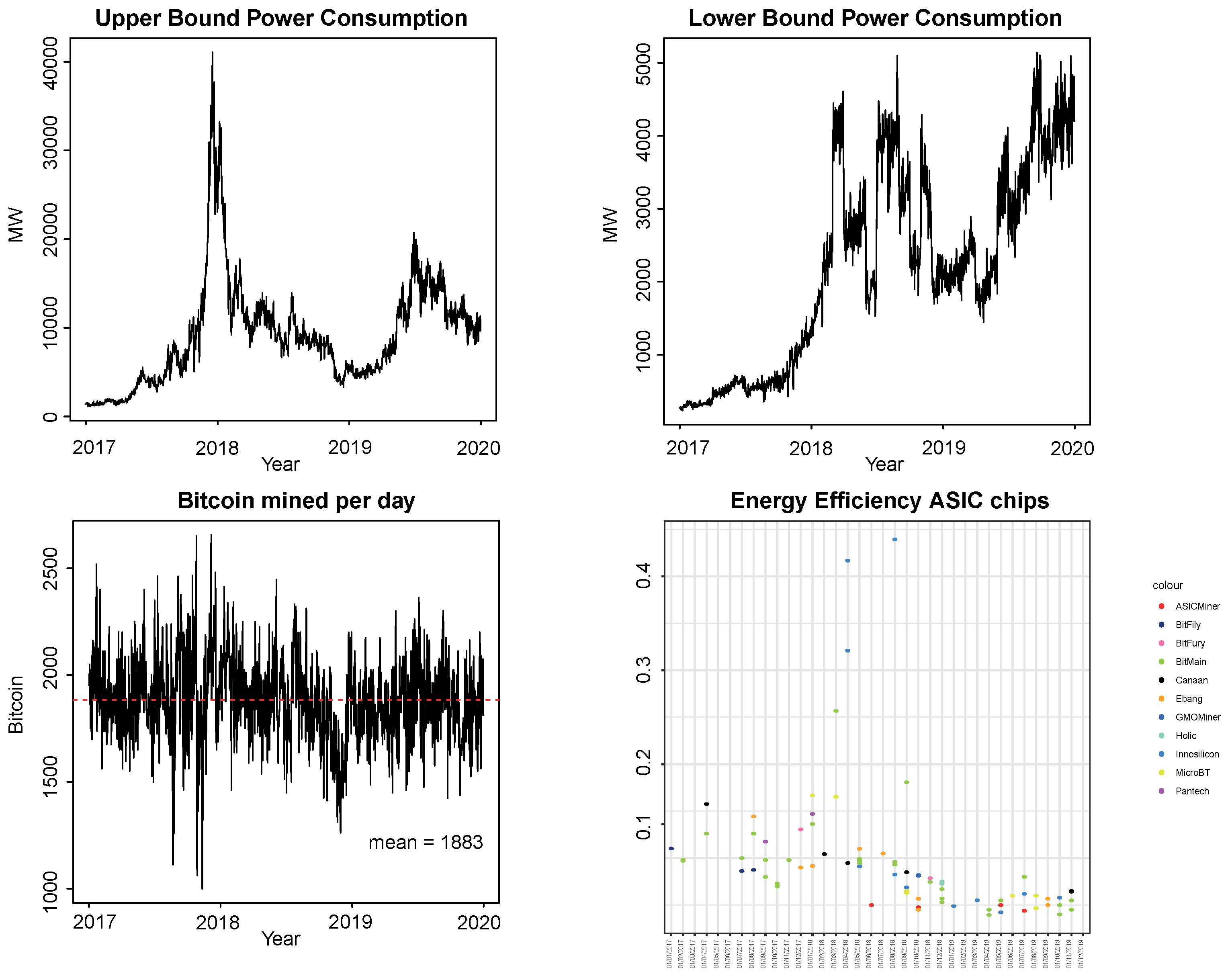
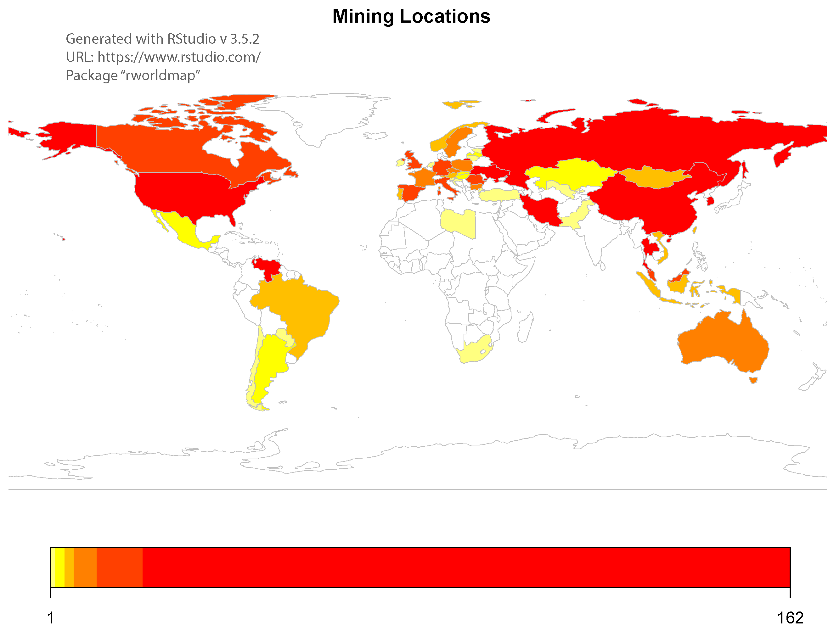
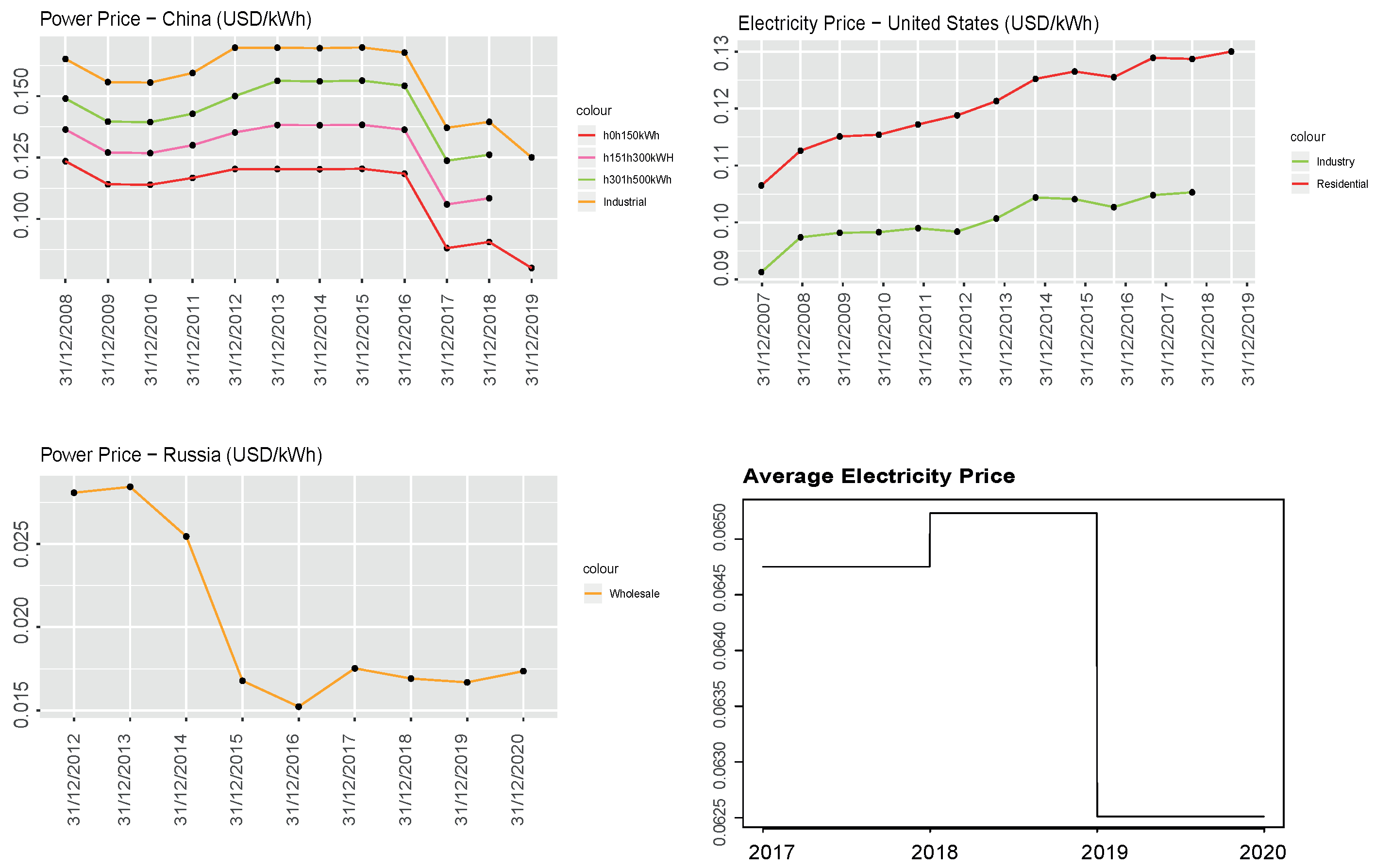
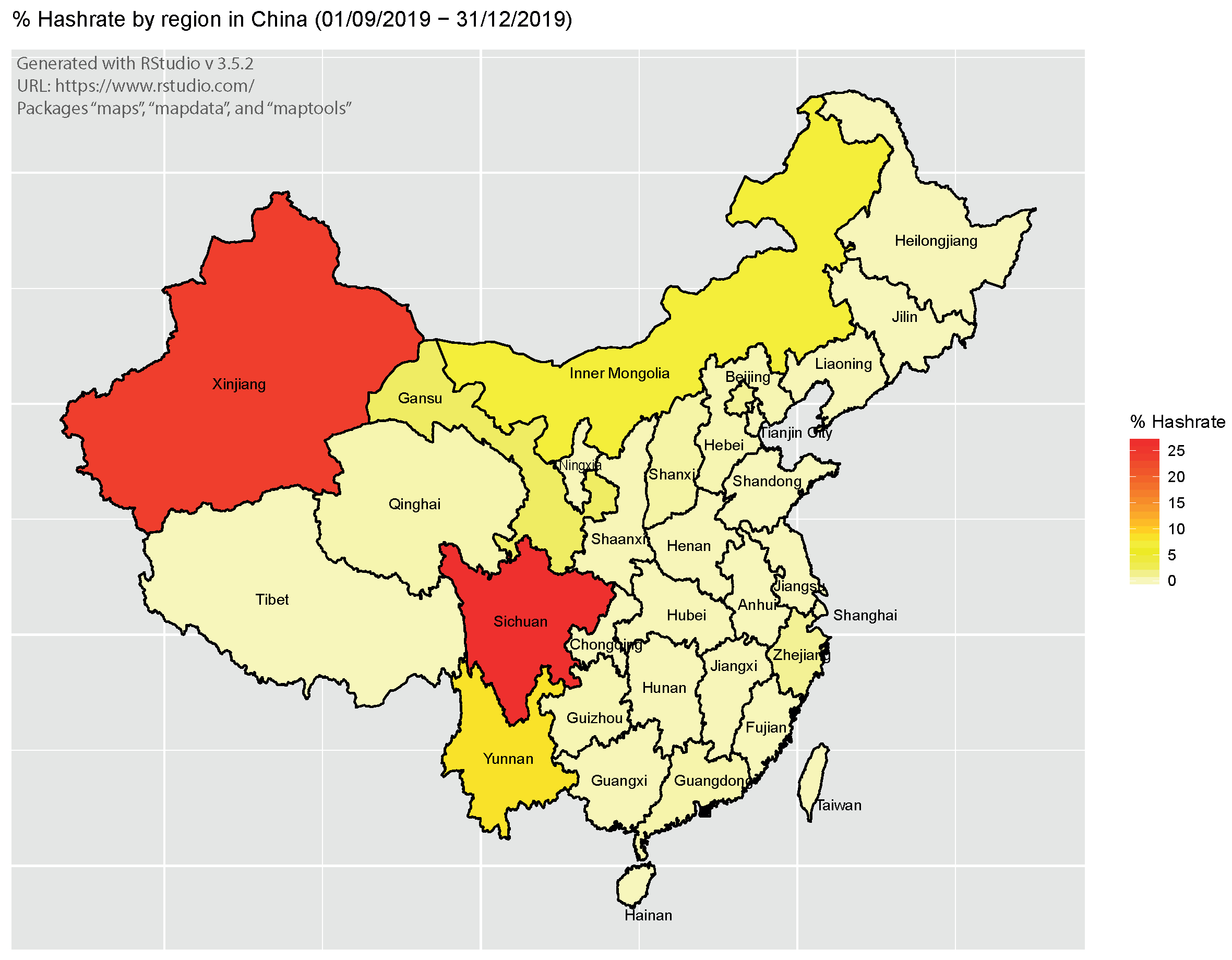
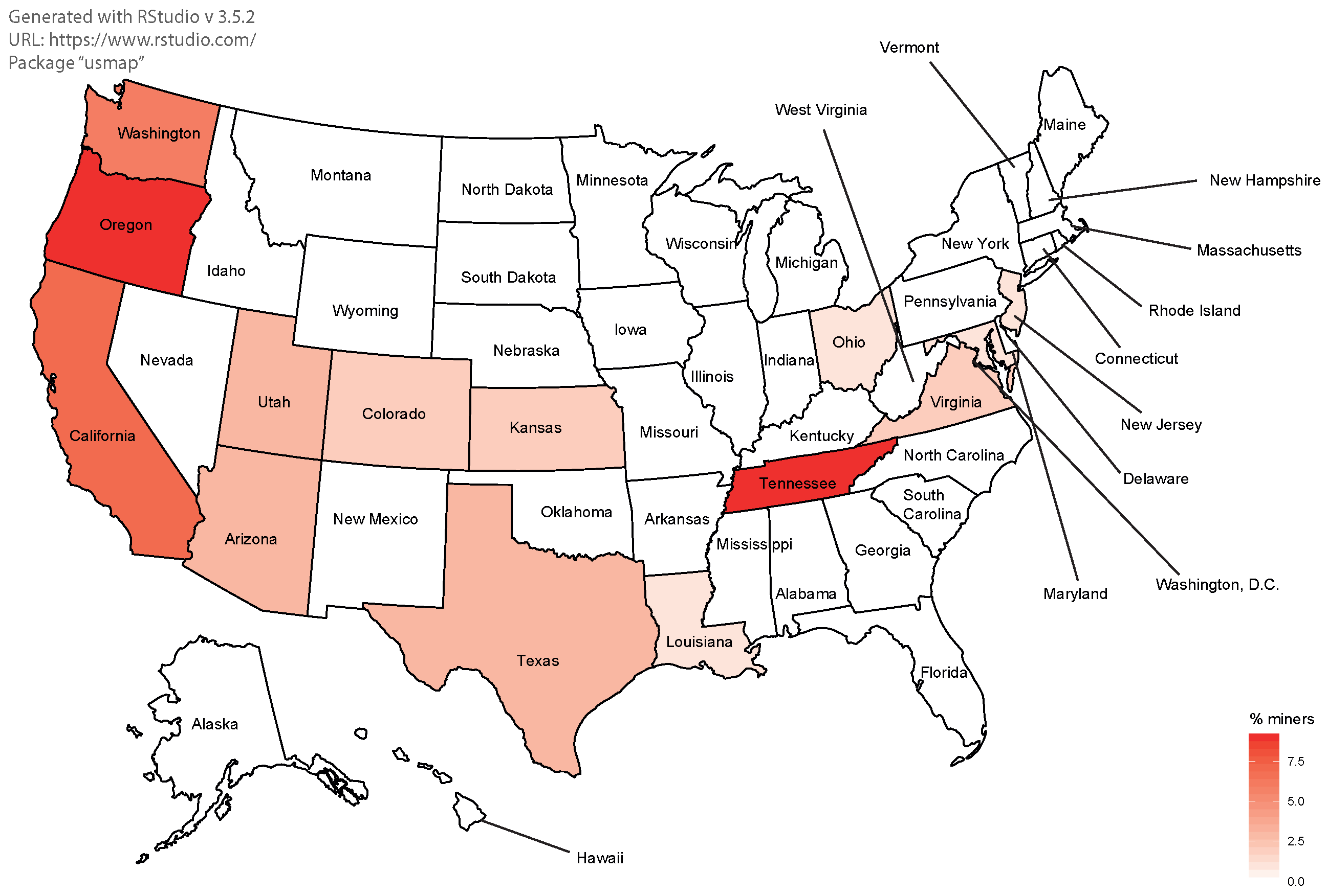
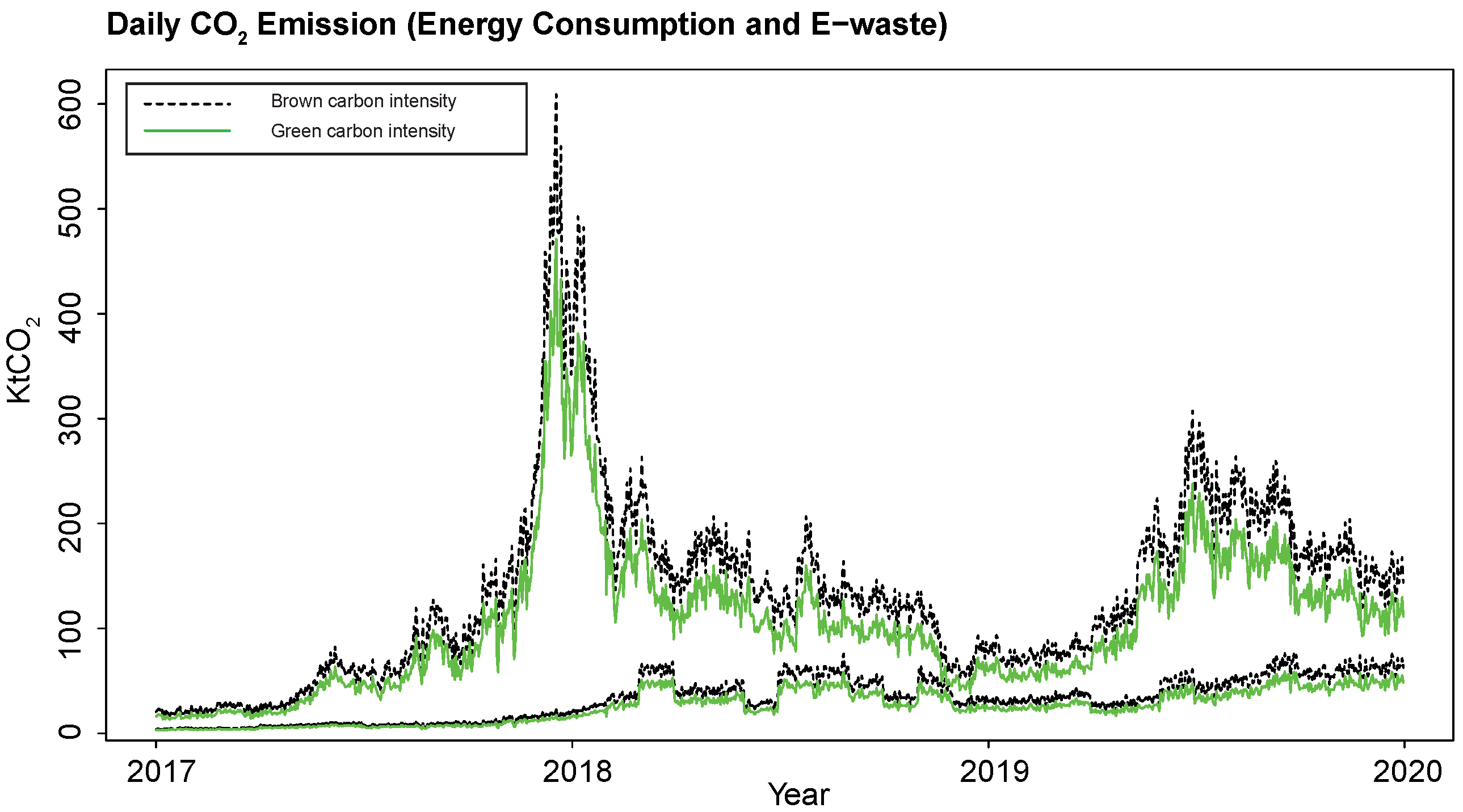
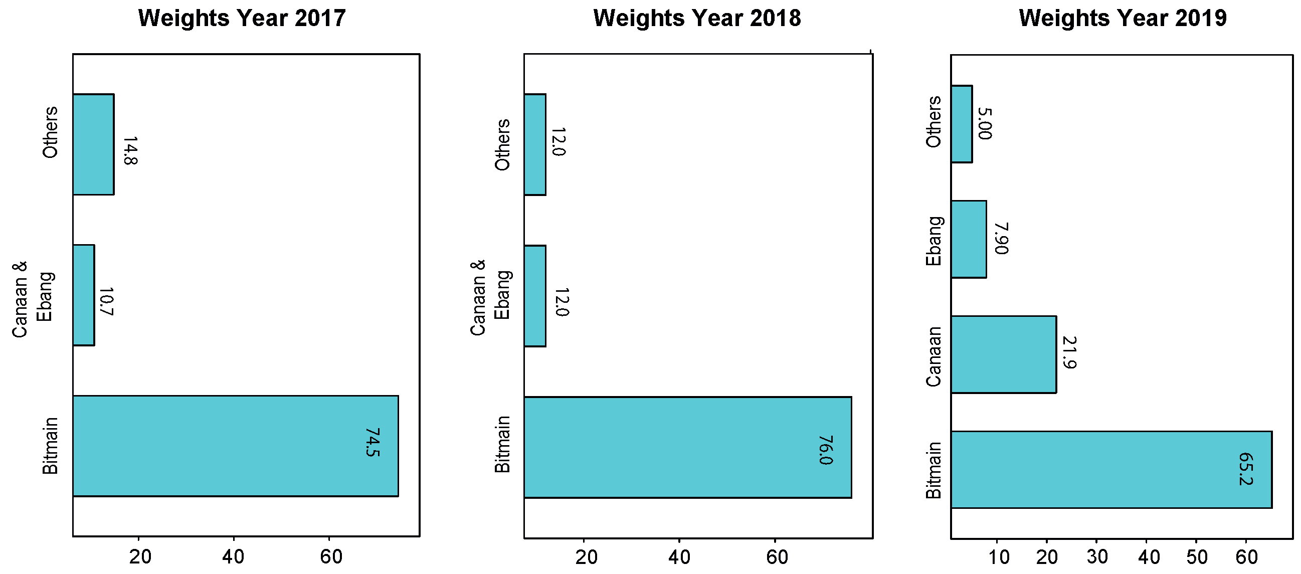
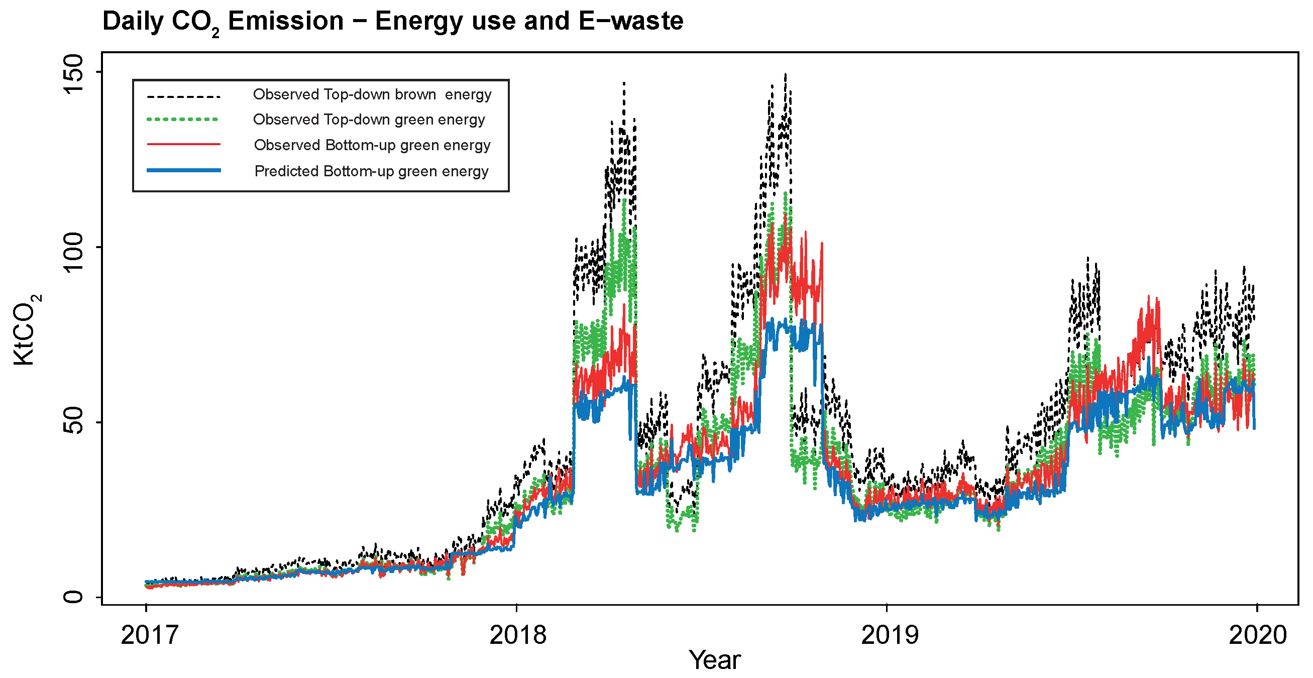
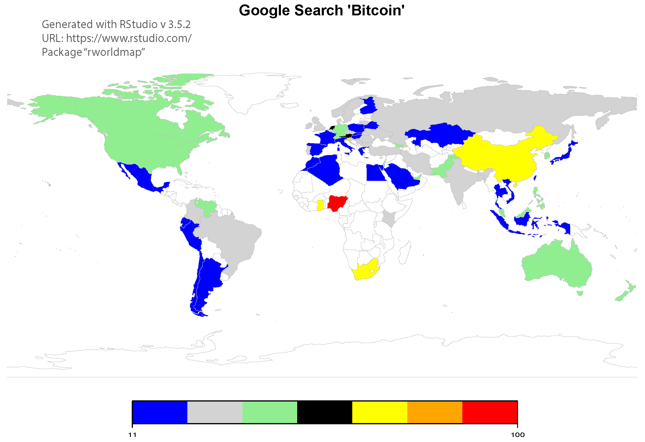
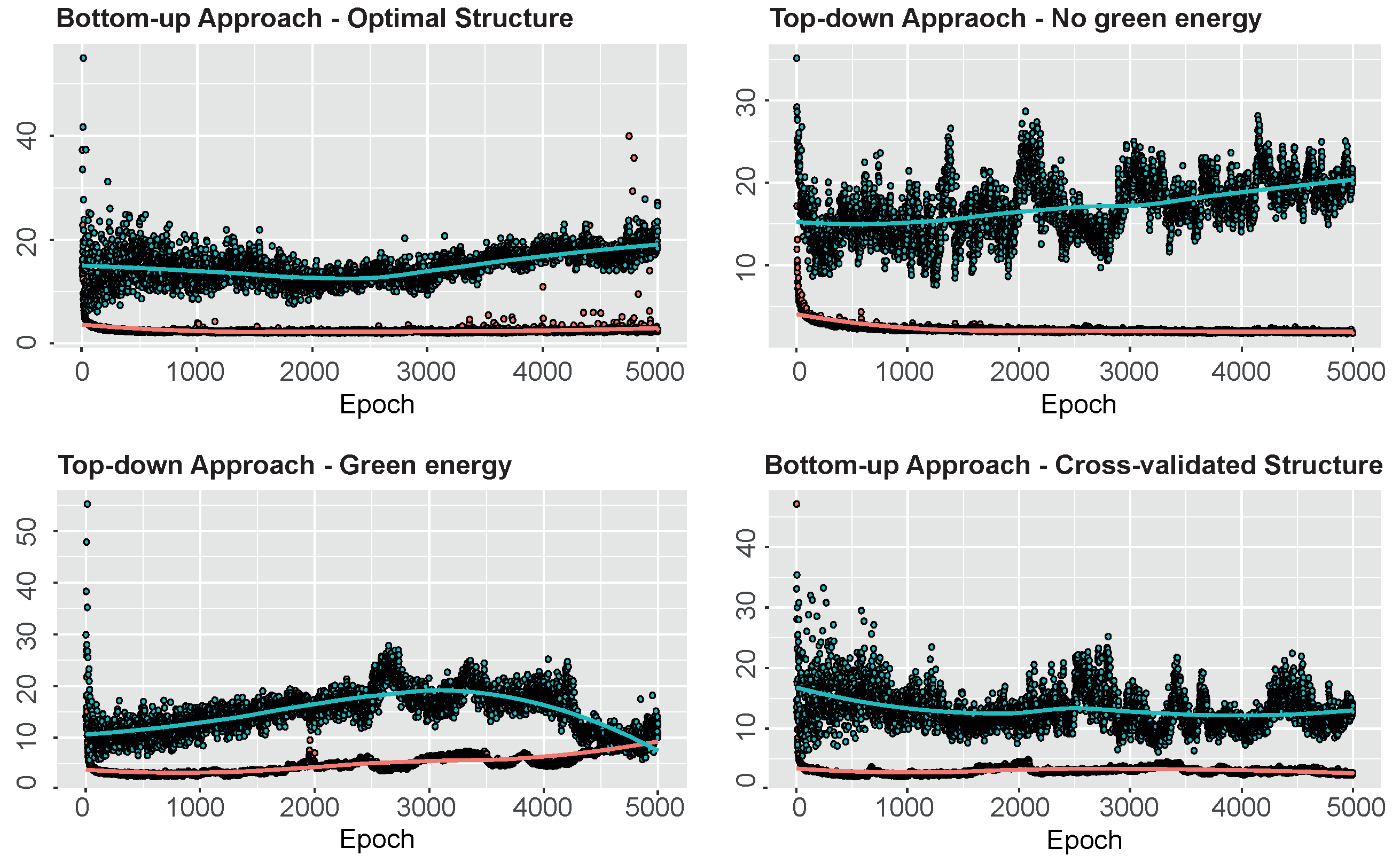
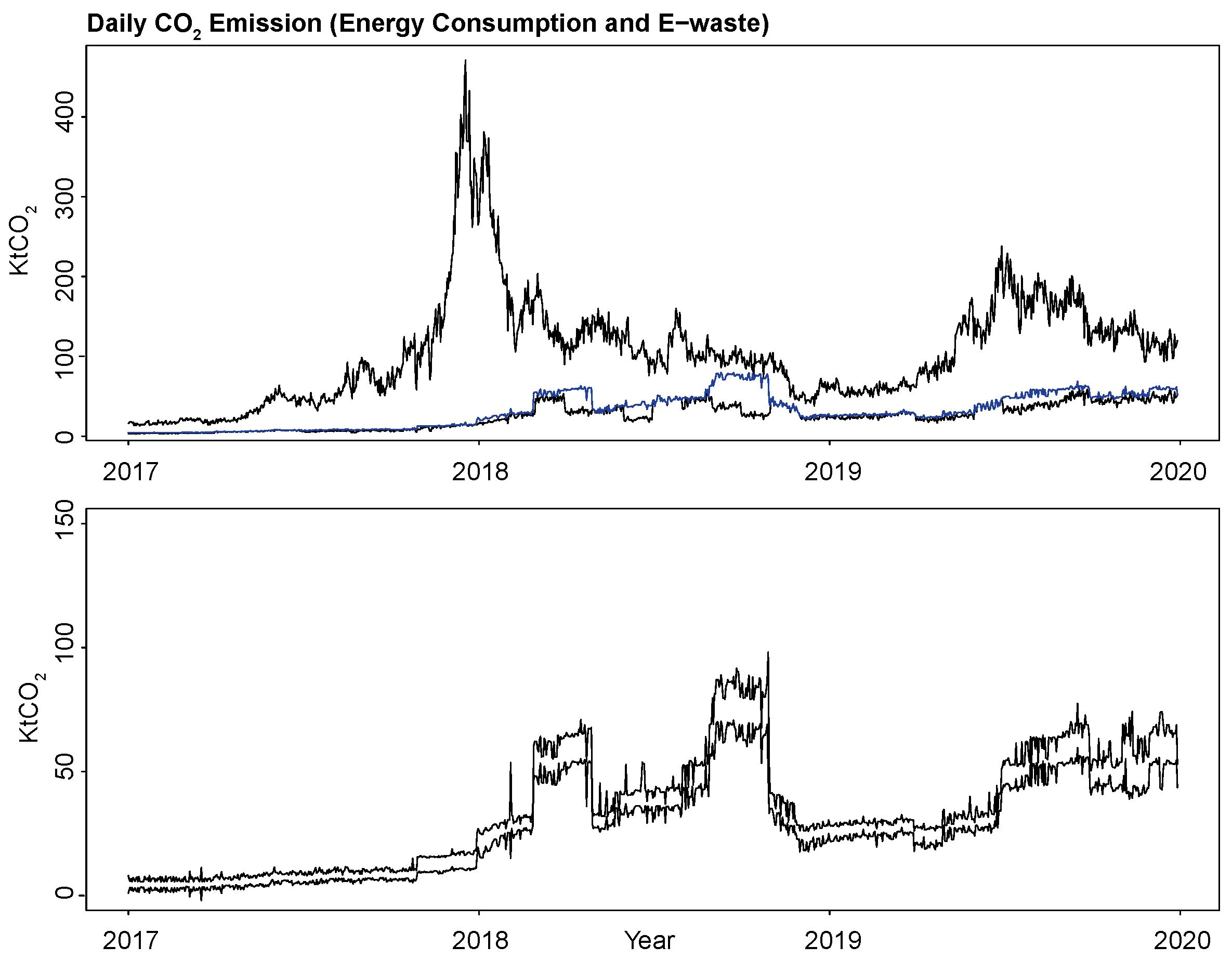
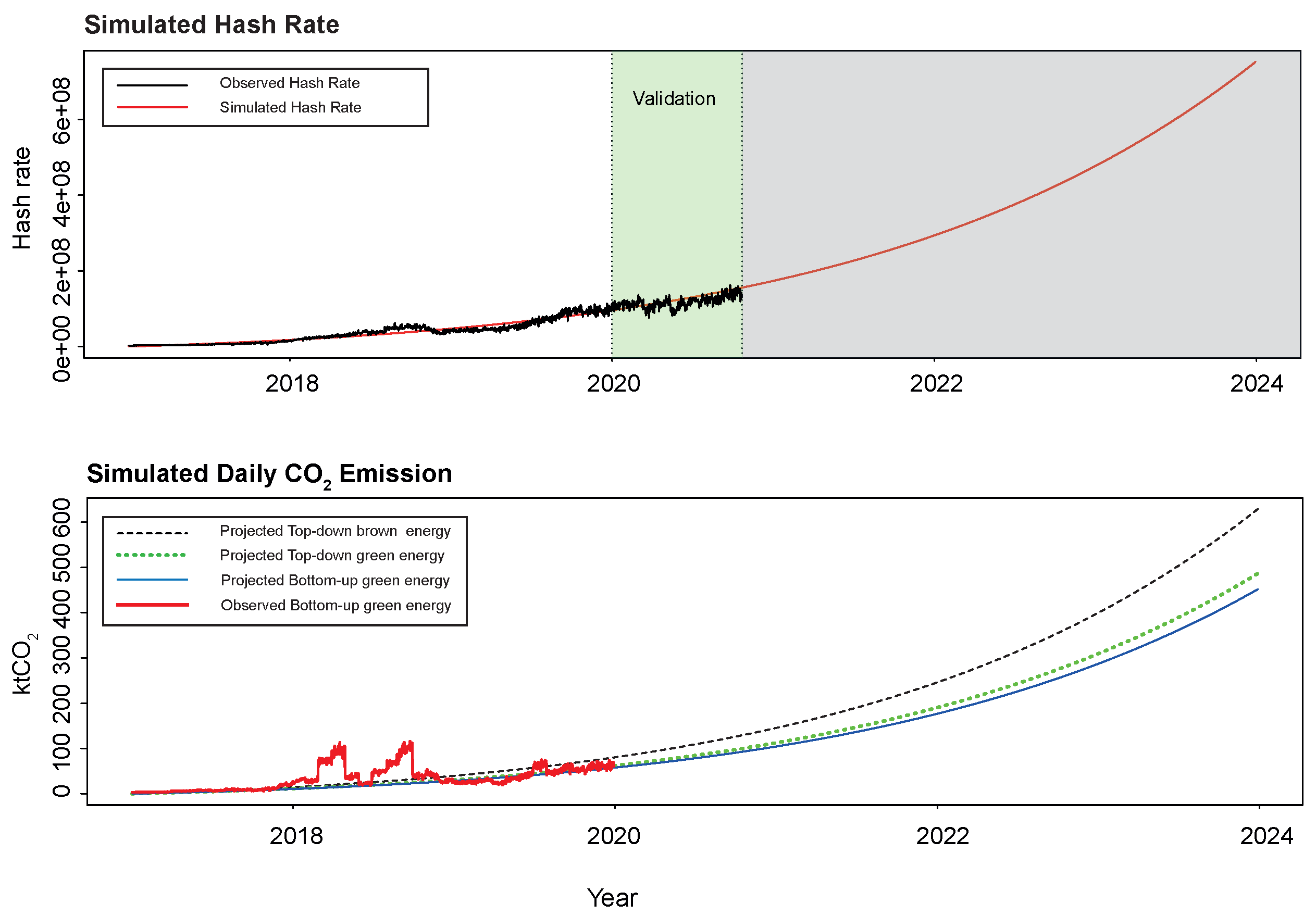
Table 1.
The table reports the descriptive statistics for the 42 input series considered. The “price” data were converted into log returns before standardizing for the training of the network. The column Shapiro–Wilk reports the p-value associated with the Shapiro–Wilk test for normality. Sources: Bloomberg, St. Louis Federal Reserve database and Google statistics webpage.
| Mean | Median | Std. Dev. | Min | Max | 0.25 Q. | 0.75 Q. | Shapiro–Wilk | |
|---|---|---|---|---|---|---|---|---|
| AUDCurncy | −2.94E-05 | 0 | 4.84E-03 | −1.80E-02 | 1.96E-02 | −3.32E-03 | 3.16E-03 | 4.53E-03 |
| EURCurncy | 8.96E-05 | 8.85E-05 | 4.10E-03 | −1.91E-02 | 1.40E-02 | −2.54E-03 | 2.53E-03 | 1.39E-03 |
| GBPCurncy | 9.82E-05 | 7.57E-05 | 5.25E-03 | −1.69E-02 | 3.00E-02 | −3.29E-03 | 2.91E-03 | 3.59E-10 |
| CADCurncy | 4.39E-05 | −0.0001498 | 4.05E-03 | −1.72E-02 | 1.66E-02 | −2.32E-03 | 2.23E-03 | 1.02E-05 |
| SGDCurncy | 9.60E-05 | 0.00014304 | 2.49E-03 | −9.98E-03 | 1.05E-02 | −1.42E-03 | 1.47E-03 | 1.62E-07 |
| CHFCurncy | 7.32E-05 | −0.000102 | 3.97E-03 | −1.46E-02 | 1.30E-02 | −2.38E-03 | 2.48E-03 | 7.75E-04 |
| JPYCurncy | 1.01E-04 | 9.14E-05 | 4.30E-03 | −1.79E-02 | 2.05E-02 | −2.47E-03 | 2.29E-03 | 1.67E-08 |
| CNHCurncy | 2.46E-06 | −8.72E-05 | 3.06E-03 | −1.74E-02 | 1.35E-02 | −1.64E-03 | 1.37E-03 | 2.67E-15 |
| CNYCurncy | −3.35E-06 | 0 | 2.52E-03 | −1.58E-02 | 1.12E-02 | −1.13E-03 | 1.24E-03 | 1.21E-15 |
| XAUCurncy | 3.58E-04 | 0.00039595 | 6.51E-03 | −2.18E-02 | 2.46E-02 | −3.48E-03 | 4.27E-03 | 8.83E-05 |
| CL1Comdty | 1.64E-04 | 0.0015186 | 1.88E-02 | −8.23E-02 | 1.37E-01 | −8.88E-03 | 1.05E-02 | 2.39E-17 |
| PL1Comdty | 9.55E-05 | 0.00023764 | 1.19E-02 | −5.25E-02 | 4.58E-02 | −6.77E-03 | 6.95E-03 | 3.28E-08 |
| LMAHDS03Comdty | 8.56E-05 | 0 | 1.07E-02 | −7.31E-02 | 5.34E-02 | −6.23E-03 | 6.22E-03 | 2.90E-13 |
| LMCADS03Comdty | 1.40E-04 | 0 | 1.06E-02 | −4.23E-02 | 4.52E-02 | −6.15E-03 | 6.38E-03 | 6.48E-08 |
| CDMNCLTIndex | 1.63E+02 | 153.5 | 5.61E+01 | 5.86E+01 | 3.30E+02 | 1.34E+02 | 1.92E+02 | 1.88E-25 |
| RWEXCLVAIndex | 4.94E+06 | 5,019,960 | 2.11E+06 | 2.38E+05 | 9.65E+06 | 3.76E+06 | 6.37E+06 | 6.11E-09 |
| RWEXCLVOIndex | 1.31E+05 | 128,133 | 4.48E+04 | 1.06E+04 | 2.40E+05 | 1.09E+05 | 1.58E+05 | 3.97E-13 |
| CAIPMOMIndex | 1.32E-01 | 0.17 | 7.04E-01 | −1.42E+00 | 1.50E+00 | −3.30E-01 | 6.10E-01 | 6.09E-12 |
| UKIPIMOMIndex | −3.46E-02 | 0 | 8.09E-01 | −3.30E+00 | 1.70E+00 | −4.00E-01 | 2.00E-01 | 1.21E-27 |
| IPCHNGIndex | 2.03E-01 | 0.14 | 5.22E-01 | −7.90E-01 | 1.52E+00 | −2.50E-01 | 5.70E-01 | 1.48E-11 |
| JNIPMOMIndex | −7.57E-02 | 0.1 | 1.67E+00 | −4.50E+00 | 2.60E+00 | −1.00E+00 | 1.10E+00 | 2.17E-17 |
| SIIPMOMIndex | 8.95E-02 | −0.3 | 4.54E+00 | −9.80E+00 | 1.01E+01 | −3.60E+00 | 3.40E+00 | 1.28E-07 |
| CAPIPDINIndex | 8.99E+05 | 906,041.5 | 4.41E+04 | 8.42E+05 | 9.50E+05 | 8.42E+05 | 9.50E+05 | 7.31E-31 |
| PITLIndex | 1.77E+04 | 17,796.58 | 7.44E+02 | 1.64E+04 | 1.89E+04 | 1.70E+04 | 1.84E+04 | 5.09E-18 |
| PCECMOMIndex | 1.42E-01 | 0.15 | 7.72E-02 | −1.10E-01 | 2.80E-01 | 1.10E-01 | 1.90E-01 | 5.55E-16 |
| PITLCHNGIndex | 4.01E-01 | 0.4 | 2.08E-01 | 0.00E+00 | 9.00E-01 | 3.00E-01 | 5.00E-01 | 3.49E-16 |
| SPXIndex | 4.70E-04 | 0.00050924 | 7.94E-03 | −4.18E-02 | 4.84E-02 | −2.17E-03 | 4.38E-03 | 3.58E-22 |
| SX5EIndex | 2.49E-04 | 0.00056771 | 8.25E-03 | −3.31E-02 | 5.29E-02 | −4.23E-03 | 5.06E-03 | 1.16E-11 |
| INDUIndex | 4.71E-04 | 0.00041741 | 8.16E-03 | −4.71E-02 | 4.86E-02 | −2.45E-03 | 4.36E-03 | 9.20E-22 |
| CCMPIndex | 6.54E-04 | 0.00071221 | 9.97E-03 | −4.53E-02 | 5.67E-02 | −2.85E-03 | 6.04E-03 | 3.79E-19 |
| SHCOMPIndex | −2.66E-05 | 0 | 1.08E-02 | −6.19E-02 | 5.82E-02 | −4.53E-03 | 5.53E-03 | 7.34E-18 |
| VIXIndex | −2.39E-05 | −0.0029895 | 8.09E-02 | −3.00E-01 | 7.68E-01 | −4.27E-02 | 3.16E-02 | 3.81E-23 |
| NKYIndex | 3.61E-04 | 0.00018195 | 8.99E-03 | −4.28E-02 | 4.12E-02 | −4.06E-03 | 5.77E-03 | 1.00E-12 |
| UKXIndex | 1.62E-04 | 0.00033114 | 7.58E-03 | −3.36E-02 | 3.00E-02 | −3.99E-03 | 4.69E-03 | 2.18E-10 |
| GoogleBitcoin | 5.02E+01 | 52 | 2.23E+01 | 8.00E+00 | 1.00E+02 | 3.40E+01 | 6.70E+01 | 2.66E-09 |
| Gold | 3.58E-04 | 0.000163 | 6.68E-03 | −2.28E-02 | 3.53E-02 | −3.22E-03 | 4.03E-03 | 2.71E-10 |
| SHASHRIndex | −2.57E-05 | 0 | 1.08E-02 | −6.19E-02 | 5.82E-02 | −4.51E-03 | 5.55E-03 | 7.43E-18 |
| IBVCIndex | −2.45E-03 | 0 | 2.30E-01 | −5.75E+00 | 4.31E-01 | −1.46E-02 | 3.08E-02 | 1.44E-49 |
| Sinopec | −2.34E-04 | −0.0003256 | 1.47E-02 | −7.47E-02 | 5.95E-02 | −7.56E-03 | 8.04E-03 | 6.97E-13 |
| FSI | −1.19E+00 | −1.219 | 1.97E-01 | −1.49E+00 | −4.71E-01 | −1.34E+00 | −1.06E+00 | 2.20E-16 |
| Average (USA) | 6.77E-04 | 0.00021563 | 1.11E-02 | −4.48E-02 | 5.49E-02 | −5.07E-03 | 6.78E-03 | 3.70E-11 |
| Average (China) | 1.40E-04 | 8.16E-05 | 1.35E-02 | −9.17E-02 | 1.38E-01 | −5.11E-03 | 5.98E-03 | 4.11E-30 |
Publisher’s Note: MDPI stays neutral with regard to jurisdictional claims in published maps and institutional affiliations. |
© 2022 by the authors. Licensee MDPI, Basel, Switzerland. This article is an open access article distributed under the terms and conditions of the Creative Commons Attribution (CC BY) license (https://creativecommons.org/licenses/by/4.0/).
Share and Cite
MDPI and ACS Style
Calvo-Pardo, H.F.; Mancini, T.; Olmo, J. Machine Learning the Carbon Footprint of Bitcoin Mining. J. Risk Financial Manag. 2022, 15, 71. https://doi.org/10.3390/jrfm15020071
AMA Style
Calvo-Pardo HF, Mancini T, Olmo J. Machine Learning the Carbon Footprint of Bitcoin Mining. Journal of Risk and Financial Management. 2022; 15(2):71. https://doi.org/10.3390/jrfm15020071
Chicago/Turabian StyleCalvo-Pardo, Hector F., Tullio Mancini, and Jose Olmo. 2022. "Machine Learning the Carbon Footprint of Bitcoin Mining" Journal of Risk and Financial Management 15, no. 2: 71. https://doi.org/10.3390/jrfm15020071