What Coins Lead in the Cryptocurrency Market: Using Copula and Neural Networks Models


1
Division of Mathematics and Computer Science, University of South Carolina Upstate, Spartanburg, SC 29303, USA
2
Department of Mathematics, University of North Carolina Asheville, Asheville, NC 28804, USA
3
Statistics Discipline, Division of Science and Mathematics, University of Minnesota-Morris, Morris, MN 56267, USA
4
Department of Finance, Ziegler College of Business, Bloomsburg University, Bloomsburg, PA 17815, USA
*
Author to whom correspondence should be addressed.
J. Risk Financial Manag. 2019, 12(3), 132; https://doi.org/10.3390/jrfm12030132
Submission received: 10 July 2019
/
Revised: 31 July 2019
/
Accepted: 5 August 2019
/
Published: 8 August 2019
(This article belongs to the Special Issue Machine Learning Applications in Finance)
Abstract
:Exploring dependence structures between financial time series has been important within a wide range of applications. The main aim of this paper is to examine dependence relationships among five well-known cryptocurrencies—Bitcoin, Ethereum, Litecoin, Ripple, and Stella—by a copula directional dependence (CDD). By employing a neural network autoregression model to avoid the serial dependence in each individual cryptocurrency, we generate residuals of the fitted models with time series of daily log-returns in percentage of the five cryptocurrencies and then we apply a Gaussian copula marginal beta regression model to the residuals to explore the CDD. The results show that the CDD from Bitcoin to Litecoin is highest among all ordered directional dependencies and the CDDs from Ethereum to the other four cryptocurrencies are relatively higher than the CDDs to Ethereum from those cryptocurrencies. This finding implies that the return shocks of Bitcoin have the most effect on Litecoin and the return shocks of Ethereum relatively influence the shocks on the other four cryptocurrencies instead of being affected by them. This allows investors to build the market-timing strategies by observing the directional flow of return shocks among cryptocurrencies.
Keywords:
Directional dependence; Copula; Neural Network; Beta regression; Cryptocurrencies; Bitcoin1. Introduction
Cryptocurrency is a digital or virtual currency that is exchanged between peers without the need of a third party. Transactions of the cryptocurrency involve no centralized authority, clearing house, or institution. For example, the first cryptocurrency, Bitcoin, operates with block chain technology, in which a transparent and secure system of accounting is used that transfers ownership. Because cryptocurrencies have exploded in value and the use of cryptocurrencies has increased for various reasons such as investment purposes, cryptocurrency has received growing attention from the media, academia, and the finance industry. Since the inception of Bitcoin in 2009, over 2000 alternative digital currencies have been developed and there have been a number of studies on the analysis of the exchange rates of cryptocurrency.
The early work on cryptocurrencies naturally concentrated on Bitcoin. Kristoufek (2013) used vector autoregression (VAR) and vector error correction (VEC) models to search for the relationship between Bitcoin’s price and the interest in Bitcoin represented by Google Trends and Wikipedia search queries, and found that there is the statistically significant bi-directional relationship between Bitcoin and Google Trends, while the relationship between Bitcoin and Wikipedia is not significant. The results also indicate that, if the price of Bitcoin increases, so does the public interest in it pushing the Bitcoin price to increase even more. Hencic and Gourieroux (2015) proposed a non-causal autoregressive process with Cauchy errors to predict the exchange rates of the Bitcoin electronic currency against the US Dollar. Dyhrberg (2016) applied the generalized autoregressive conditional heteroskedasticity (GARCH) model to examine Bitcoin’s capabilities of being a financial asset and found that it is more characteristic of an asset rather than a currency and it also possesses risk management and hedging capabilities. Gkillas and Katsiampa (2018) studied the tail behavior of returns of five major cryptocurrencies (Bitcoin, Bitcoin Cash, Ethereum, Litecoin, and Ripple) using extreme value analysis and estimating Value-at-Risk and Expected Shortfall as tail risk measures. They found that Bitcoin Cash is the riskiest, while Bitcoin and Litecoin are the least risky cryptocurrencies. Meanwhile, Katsiampa (2017) compared GARCH-type models to examine which conditional heteroskedasticity model can describe the Bitcoin price volatility better and proposed the AR-CGARCH model to estimate the volatility of Bitcoin.
Despite all these various efforts to analyze the forecasting performances of cryptocurrencies, understanding the relationship among cryptocurrencies is important for investors whose investment portfolios contain a portion of cryptocurrencies as well as for policymakers whose role is to maintain the stability of financial markets. Bação et al. (2018) used a VAR modelling approach to investigate transmission between cryptocurrencies and Corbet et al. (2018) explored the dynamic relationships between cryptocurrencies and other financial assets. Katsiampa (2019) employed an asymmetric Diagonal BEKK model (the acronym comes from synthesized work on multivariate models by Baba, Engle, Kraft and Kroner); studied the volatility dynamics of Bitcoin, Ethereum, Litecoin, Ripple, and Stellar to examine interdependencies within cryptocurrency markets for those five major cryptocurrencies; and found evidence of significant interdependencies in the cryptocurrency market. Given the dramatic Bitcoin price rise in 2016 and 2017 and fadeaway in 2018, Bouri et al. (2019a) detected multiple periods of explosivity in cryptocurrencies and investigated whether price explosivity in one cryptocurrency affects the explosivity of other cryptocurrencies using the generalized supremum augmented Dickey–Fuller test of Phillips et al. (2015) and the logistic regression. They revealed evidence of co-explosivity and showed the probability of the explosivity in one cryptocurrency generally depends on the presence of explosivity in other cryptocurrencies. Bouri et al. (2019b) studied the presence of herd investing behavior in the cryptocurrency market. Results from the static model inspired by the approach of Chang et al. (2000) suggest no significant herding. However, with a time-varying rolling-window approach (Stavroyiannis and Babalos 2017), they found significant herding behavior and showed that the cryptocurrency market is subject to herding behavior that tends to occur as uncertainty increases.
Instead of using aforementioned approaches to examine the association and/or causality between financial time series, using a copula-based approach, however, has several attractive properties and copula models have been widely used to model dependence between financial time series (Cherubini et al. 2011). Among several references on dynamic dependence using copulas, Masarotto and Varin (2012) developed the class of Gaussian copula models for marginal regression analysis of non-normal dependent observations. This class provides a natural extension of traditional linear regression models with normal correlated errors. Ferrari and Cribari-Neto (2004) proposed a beta regression model for continuous variables that assumes values in the standard unit interval as practitioners often encounter bounded time series consisting of rates or proportions in practice, and Guolo and Varin (2014) proposed a practical approach to analyze bounded time series through a beta regression model. Using the Gaussian copula marginal regression method by Masarotto and Varin (2012) and the beta regression model by Guolo and Varin (2014), Kim and Hwang (2017) proposed a new copula directional dependence and explored a relationship between two financial time series via the Gaussian copula marginal beta regression model.
In this paper, we explore directional dependence among the five well-known cryptocurrencies using the Gaussian copula beta regression model and neural networks. First, we apply a neural network autoregression model to the data and generate residuals. Through this procedure we avoid the serial dependence in the component of a cryptocurrency (Kojadinovic and Yan 2010). Then, the two sets of residuals are transformed to two uniform distributions, and we perform directional dependence via the Gaussian copula marginal beta regression.
Our proposed approach provides several advantages. First, it is common that financial asset returns are generally fat-tailed and have negative skewness and that financial time series volatility is correlated in a non-Gaussian way. In addition, due to the occurrence of extreme observations and the complex structure of the dependence among asset returns, traditional approaches often fail to incorporate the influences of asymmetries in individual distributions and in dependence. By introducing a copular function linking univariate marginals to their multivariate distribution, these issues can be treated properly.
Secondly, our approach allows us to examine the direction of contemporary dependences among return series rather than dynamic dependences and also to obtain the more randomized residuals for the input of our copula model by employing the neural network autoregression model. We can apply GARCH models to generate the marginal distribution of the data. However, we show that the fitting of the GARCH to return series of cryptocurrencies is inferior to the neural network model. The residuals obtained from traditional time series analysis such as GARCH and/or VAR may be contaminated by other explainable portions of the volatility of the return series, but the neural network model allows a great deal of flexibility and complexity in identifying directional dependence for the joint marginal distributions.
Finally, the proposed method is based on the copula regression model using a beta regression, which can effectively and flexibly detect nonlinear relationships. To the best of our knowledge, our paper is the first study to apply this methodological approach to the cryptocurrency data and this paper contributes to the existing literature by investigating the directional connections between major cryptocurrencies.
The remainder of this paper is organized as follows. Section 2 describes the neural network autoregression model, directional dependence by copula, and Gaussian copula marginal beta regression. In Section 3, we illustrate the proposed method on the five cryptocurrencies. Section 4 concludes the paper with some discussions.
2. Methods
2.1. Neural Network Autoregression Model
Neural networks (NNs) have been vigorously promoted in the computer science literature for solving a wide variety of scientific problems, and recently many people have started to investigate whether NNs are useful for tackling their various research problems (Faraway and Chatfield 1998). A brief introduction of NNs can be found in the works of Hertz et al. (1991) and Ripley (1996), and financial perspectives are provided by Azoff (1994) and Kuan and White (1994) among others.
In time series forecasting, lagged values of the time series can be used as inputs to a neural network just as we use lagged values in a linear autoregression model, and we want to predict future observations by using some functions of these past lagged values of observations. One key point about NNs is that this function need not be linear, so that an NN can be considered as a nonlinear autoregressive model. We call this a neural network autoregression or NNAR model.
We consider one popular form of NNs called the feed-forward networks with one hidden layer. To be specific, the nonlinear feed-forward neural network model for lagged time series can be written as
where L is the lag order, f is a neural network with H nodes in the hidden single layer, and the error process is assumed to be homoscedastic. The neural network model with L lags and H nodes is denoted by NNAR(L,H). For example, an NNAR(9,5) model is a neural network with the last nine observations used as inputs for forecasting the output , and with five neurons in the hidden single layer. An NNAR() model is equivalent to an ARIMA() model but without the restrictions on the parameters to ensure stationarity.
The model parameters L and H are determined automatically by default values, i.e., L by the optimal value according to the Akaike information criterion (AIC) for a linear model and H by half of the number of input values plus one. After fitting the neural network model in Equation (1) to the data, the fitted values, , are the predicted values which can be written as
The term denotes a value randomly drawn from normal distributions, which can be used for obtaining prediction intervals. We have because we do not need predicted values for . The residuals can be written as
The residuals, , can be considered to be not serially correlated. In the preprocessing step to explore a copula directional dependence between two financial time series, the autocorrelation in the time series data should be modeled and removed. However, we find that the fitting of the GARCH or VAR to return series of cryptocurrencies is inferior to the neural network model. The residuals obtained from traditional time series analysis such as GARCH may be contaminated by other explainable portions of the volatility of the return series, but the neural network model allows a great deal of flexibility and complexity in identifying directional dependence for the joint marginal distribution. We adopt the aforementioned neural network approach for estimating nonlinear autocorrelations in the data by using the nnetar function in R package forecast by (Hyndman et al. 2019).
2.2. Copula and Directional Dependence
A copula is a multivariate distribution function defined on the unit with uniformly distributed marginals. It is a useful approach for understanding and modeling dependent random variables to extract the dependence structure of random variables from the joint distribution function. In this paper, we focus on a bivariate (two-dimensional) copula, where . A 2-dimensional copula is a function with the following properties:
- For all , if at least one coordinate of is 0;
- , , for and
- C is 2-increasing (see Nelsen 2006).
Sklar (1973) showed that any bivariate distribution function, , can be represented as a function of its marginal distributions of X and Y, and , by using a two-dimensional copula . More specifically, the copula may be written as
where u and v are the continuous empirical marginal distribution functions and , respectively. It is clear that the copula determines the dependency structure between two random variables X and Y. Therefore, the copula function represents how the function is coupled with its marginal distribution functions, and . Moreover, since and have uniform distributions on , the copula is independent of marginal distributions and any one-to-one transformations of them.
Sungur (2005) defined the concept of directional dependence in bivariate regression setting by using copulas and considered general measurements of the directional dependence. Let be a random pair with uniform marginals on the and their copula C. Let denote the conditional distribution function for V given as
The copula regression function of V given U, denoted by , is the conditional expectation of V given , which can be expressed by the copula as
The directional dependence from U to V is defined by using the copula regression function on V as
which can be interpreted as the proportion of total variation of V that has been explained by the copula regression of V on U. In similar way, we can define the copula regression function of U given V
where is the conditional distribution function for U given
Then, the directional dependence from V to U is defined by using the copula regression function on U as
Note that, if U and V are independent, and and are equal to 0.5, which implies that the directional dependence in Equations (2) and (3) can be interpreted as a measure of deviation from independence. Moreover, we can compare the two directional dependences to identify which copula regression can explain more variances and has higher prediction capabilities. Thus, copula models have been widely used to model dependence between macroeconomic and financial time series (Cherubini et al. 2011).
2.3. Gaussian Copula Marginal Beta Regression
Proposed by Ferrari and Cribari-Neto (2004), the beta regression for time series assumes that the dependent variable in the standard unit interval given is beta-distributed, , with the mean parameter and the precision parameter . It follows that the density function of is
where is the gamma function. Dependence of the response on the covariates is obtained by some useful link function such as a logit function for the mean parameter,
The parameters and can be estimated based on maximum likelihood approaches. By using the beta distribution, we can model a wide variety of distributions with various locations and shapes over bounded intervals (see Ferrari and Cribari-Neto 2004; Masarotto and Varin 2012; and Guolo and Varin 2014 for more details).
To model directional dependencies by copula, it is necessary to determine an appropriate and efficient parametric form of the copula regression function for the inference of a dependence structure from data. Among several references on dynamic dependence using copulas, Jondeau and Rockinger (2006) proposed the copula-GARCH model of conditional dependencies, and following the Sungur (2005) general measures for the directional dependence in joint behavior, Kim and Hwang (2017) proposed a copula directional dependence (CDD) to measure a directional dependence between two financial time series by using the Guolo and Varin (2014) marginal extension of the beta regression model for time series and the cumulative distribution function of a normal variable. Kim and Hwang (2017) used a beta logit function with one continuous covariate by utilizing the Gaussian copula regression model. Before applying a Gaussian copula beta regression model with a single continuous covariate to financial data, they preprocessed the financial data exhibiting conditionally heteroskedasticity to the white noise process by employing an asymmetric GARCH model.
Now, we show how to estimate the CDD between two cryptocurrencies. Let and be two cryptocurrency time series. Assume that NNARs are fitted to generate the residuals, and . Through doing this procedure, we try to avoid the serial dependence in the component cryptocurrencies. By using the empirical cumulative distribution function, the two sets of residuals are transformed to two random variable data, and , in . We perform the directional dependence by the Gaussian copula marginal beta regression model fitted. Thus, we assume that follows a beta distribution with the mean parameter and precision parameter . The dependence of the response on the covariate is obtained by assuming a logit model for the mean parameter
so that and with the correlation matrix of the errors corresponding to the white noise process. Then, the directional dependence is obtained by
We use Gaussian copula marginal regression R package gcmr (Masarotto and Varin 2017) and choose beta marginal distribution to find the estimates of from Gaussian marginal regression. With these estimates of and the covariate , we compute and then calculate and . With these computed values, we compute the estimation of in Equation (4). In a similar way, the directional dependence is obtained.
3. Data Analysis
3.1. Data and Summary Statistics
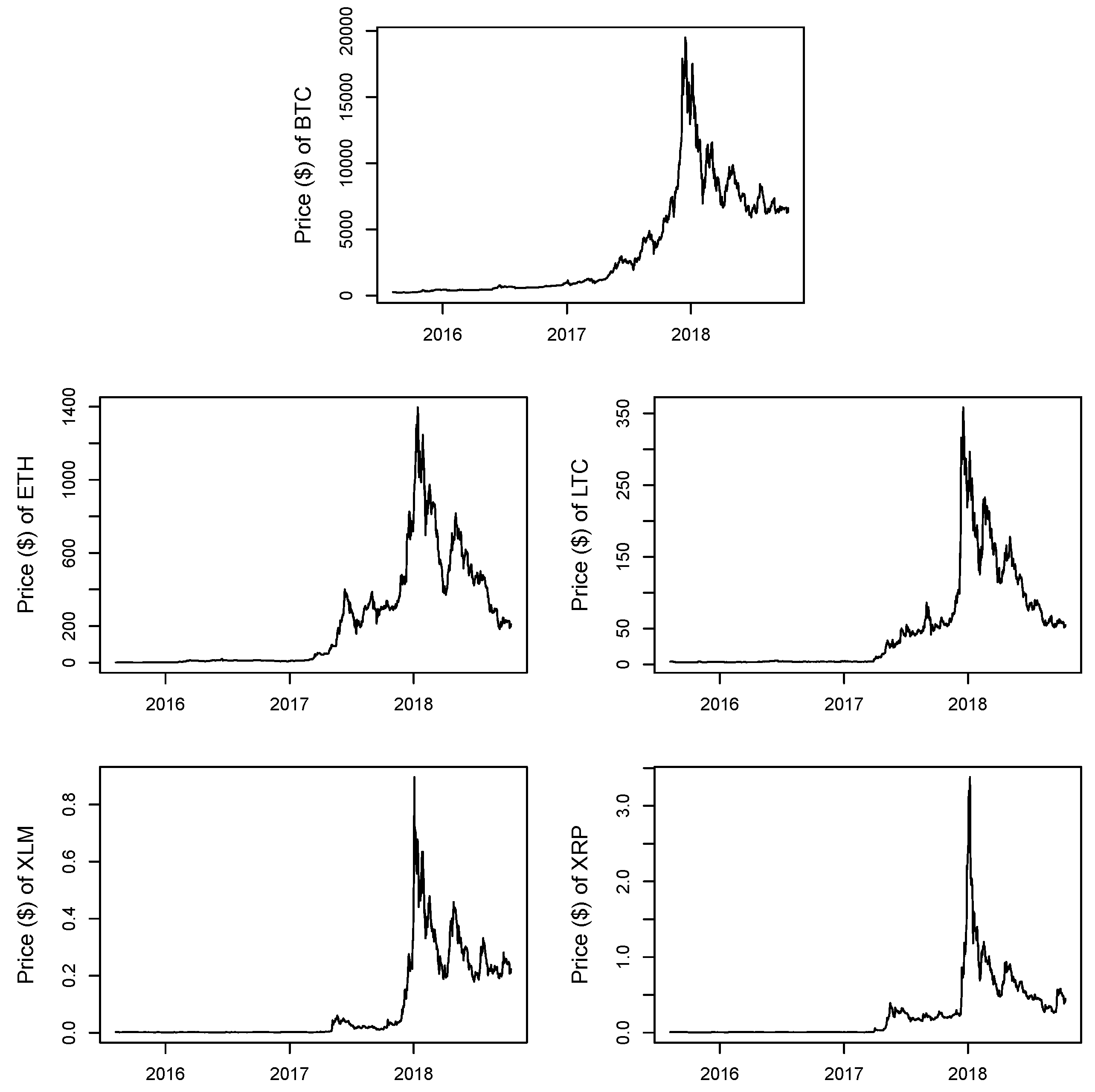
We apply the proposed method to five cryptocurrencies daily data consisting of Bitcoin (BTC), Ethereum (ETH), Litecoin (LTC), Stella (XLM), and Ripple (XRP). The data are obtained from a financial website (https://coinmarketcap.com/coins/) with time series spanning from 8 August 2015 to 15 October 2018. The dataset consists of the daily historical prices and volumes of the five cryptocurrencies. The plot of daily prices of the five cryptocurrencies is given in Figure 1. The five prices show the same pattern that, after an unprecedented boom in 2017, the prices collapsed from their peak in January 2018. For analysis, we use daily log-returns in percentage, so that the daily log-returns of Bitcoin, Ethereum, Litecoin, Stella, and Ripple are denoted as LBTC, LETH, LLTC, LXML, and LXRP, respectively. Table 1 and Table 2 provide descriptive statistics for the five daily log-returns in percentage and their correlation coefficients.
In general, daily log-returns are the fat-tail distributions, one of the common characteristics found in the return series of financial assets. Based on the kurtosis statistics in Table 1, the fat-tailed distribution is observed in all five cryptocurrencies, although the degree of the fat-tail is quite different among them. LBTC and LETH have a similar degree, while LXRP has the highest. As opposed to the kurtosis, the skewness is generally positive except LBTC, which is a bit negatively skewed. This is an interesting fact because most of financial assets’ returns show a negative skewness. This might be explained by the fact that the most recent bull market period in the crypto market, late 2017 to early 2018, is covered in the data period and the positive returns during the period dominate the negative returns before and after the bull market in terms of the magnitude of the size. This observation can be supported by the minimum and maximum value of log-returns.
Pearson’s correlation coefficients, r and coefficients of determination, among the five cryptocurrencies are shown in Table 2. Generally, the correlation coefficients are high as expected because this so-called “BTC-coupling” phenomenon is quite well-known given the dominant role of the BTC in the market. The highest correlation pair is between BTC and LTC, 0.591, and the next is between XLM and XRP, 0.540. Given the relationship of the pairs, this is expected since LTC is a spin-off project of BTC and XLM is a spin-off project of XRP. Similarly, ETH tends to have lower coefficients with the other cryptocurrencies, which supports the fact that the ETH project has started rather independently unlike the ones trying to improve original blockchain projects such as the LTC–BTC and XLM–XRP pairs. The results of Table 1 and Table 2 show a clear indication that the return series of cryptocurrencies are non-normal distributions and, thus, approaches other than the ones assuming normality should be explored. In addition, the linearity, another assumption, is easily threatened in this kind of time series data. Though several approaches other than ordinary least squares as well as its remedy versions are introduced to address the dependence among time series data, the Gaussian copula marginal beta model along with the neural network model allows us to remove the serial dependence among financial time series data and to examine the directional dependence using the residuals generated by the neural network autoregression models.
3.2. Results
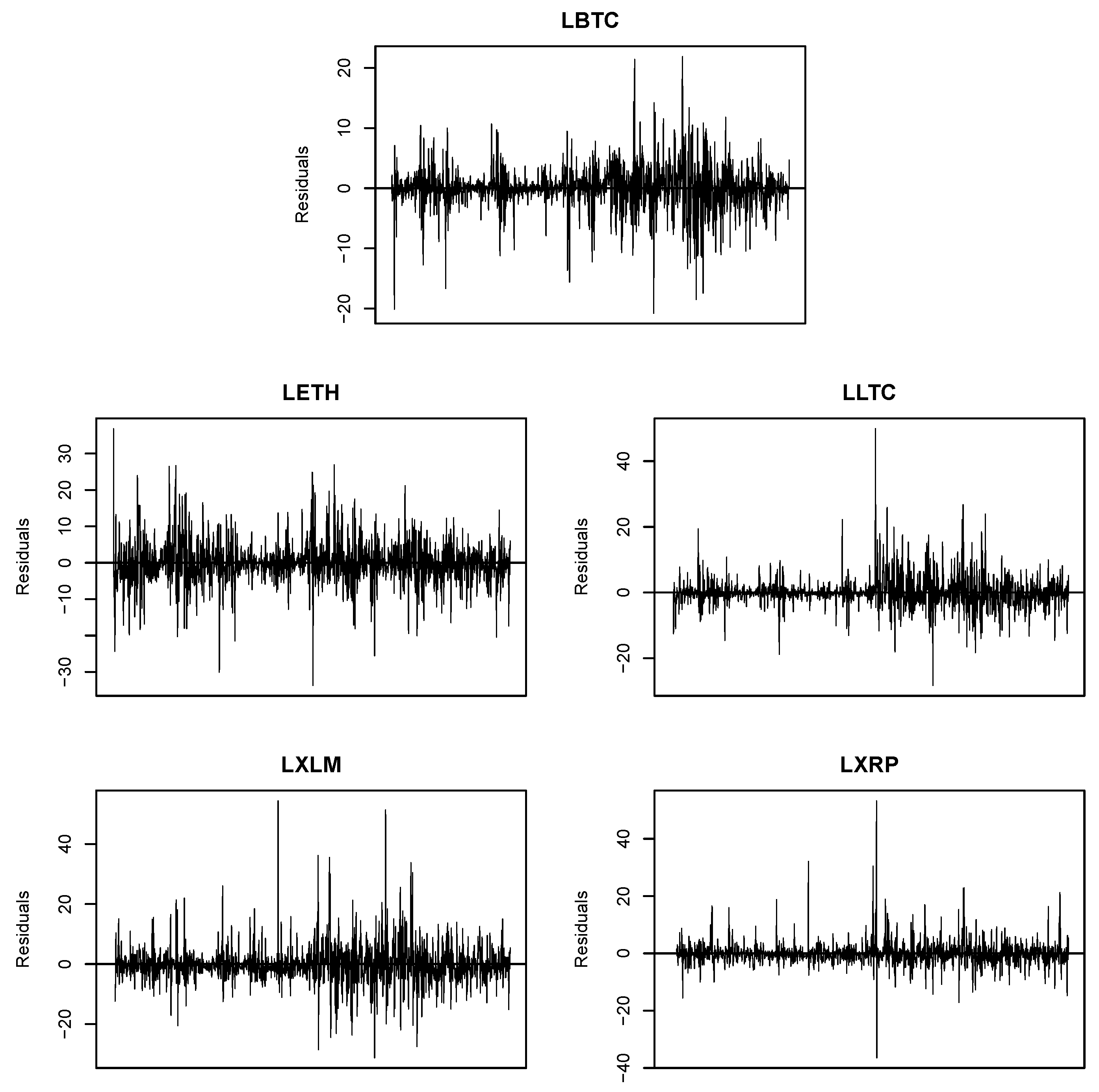
The autocorrelation in the time series data should be modeled and removed before estimating a copula direction dependence. We adopt the neural network approach for estimating nonlinear autocorrelations in the data. The neural network autoregression models used for the five daily log-returns in percentage are given in Table 3. Among them, the XRP log-return is more consistently influenced by past log-returns (18 lagged time series (L = 18)) with the more complicated model structure with 10 hidden layers (H = 10) while the BTC log-return is with L = 1 and H = 1. Figure 2 shows the residuals of log-returns using the neural network autoregression models. The results show that the residuals are close to a white-noise signal, implying that the NNAR models effectively remedy the serial correlation of the time series data. Using the residuals generated by the NNAR models, the contemporary directional dependencies among the five cryptocurrencies are examined using the Gaussian copular beta regression model, and the results are summarized in Table 4 and Figure 3. The results are obtained as follows: The total observation of log-returns for each cryptocurrency we consider is . We take 70% of the total observations () with random sampling from and perform 1000 replications with sample size for computing copula directional dependence. We compute 1000 difference of , which is denoted by Diff. With these 1000 values, we perform the bootstrapping method so that we have 3000 bootstrap replicates to compute Estimate (Diff), Bias (Diff), Std. Error (Diff), MSE (Diff), and 95% bootstrapping confidence interval of Diff.
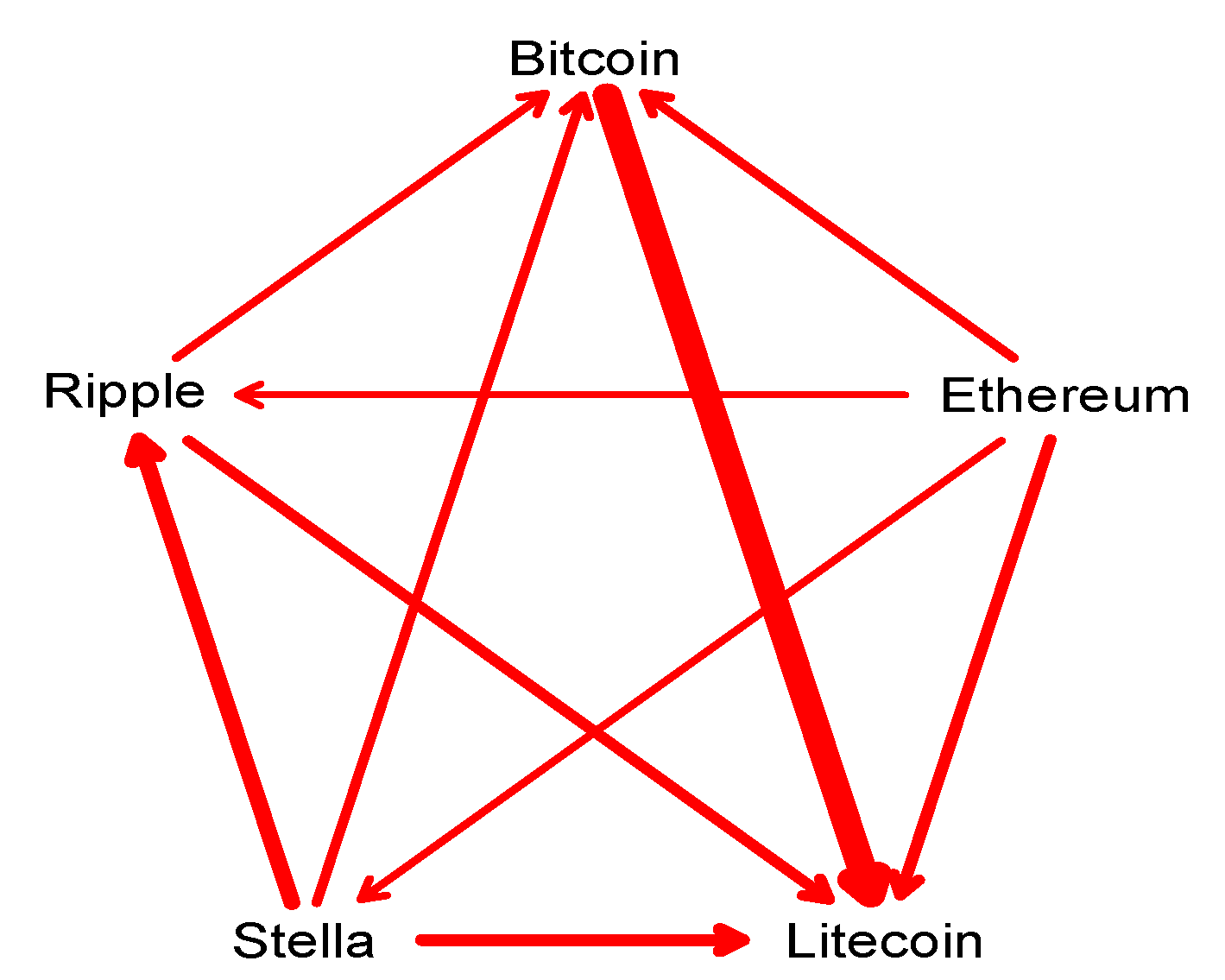
The results in Table 4 show that, overall, moderate directional dependence exists among the five cryptocurrencies. It appears that the Bitcoin–Litecoin pair has the greatest dependence, followed by the Ripple–Stella pair, and, among all ordered directional dependencies, the CDD from Bitcoin to Litecoin is highest (0.3890) and the CDD from Ripple to Ethereum is lowest (0.0893). As expected, the dependence between Bitcoin and Litecoin is generally stronger than among others because Litecoin is a spin-off project of Bitcoin. The CDD from Stellar to Ripple is relatively high (0.2208) among all pairwise directional dependencies and the CDDs from Ethereum to the other four cryptocurrencies are higher than the CDDs to Ethereum from those cryptocurrencies. To better visualize the structure of directional dependence, Figure 3 only provides the stronger CDD between pairwise directions. The thickness of the arrows reflects the strength of copula directional dependence, with thicker arrows indicating stronger pairwise directional dependence. This finding implies that the return shocks of Bitcoin have the most effect on Litecoin, Stellar has relatively stronger impact on Ripple, and the return shocks of Ethereum relatively influence the shocks of the other four cryptocurrencies instead of being influenced by them.
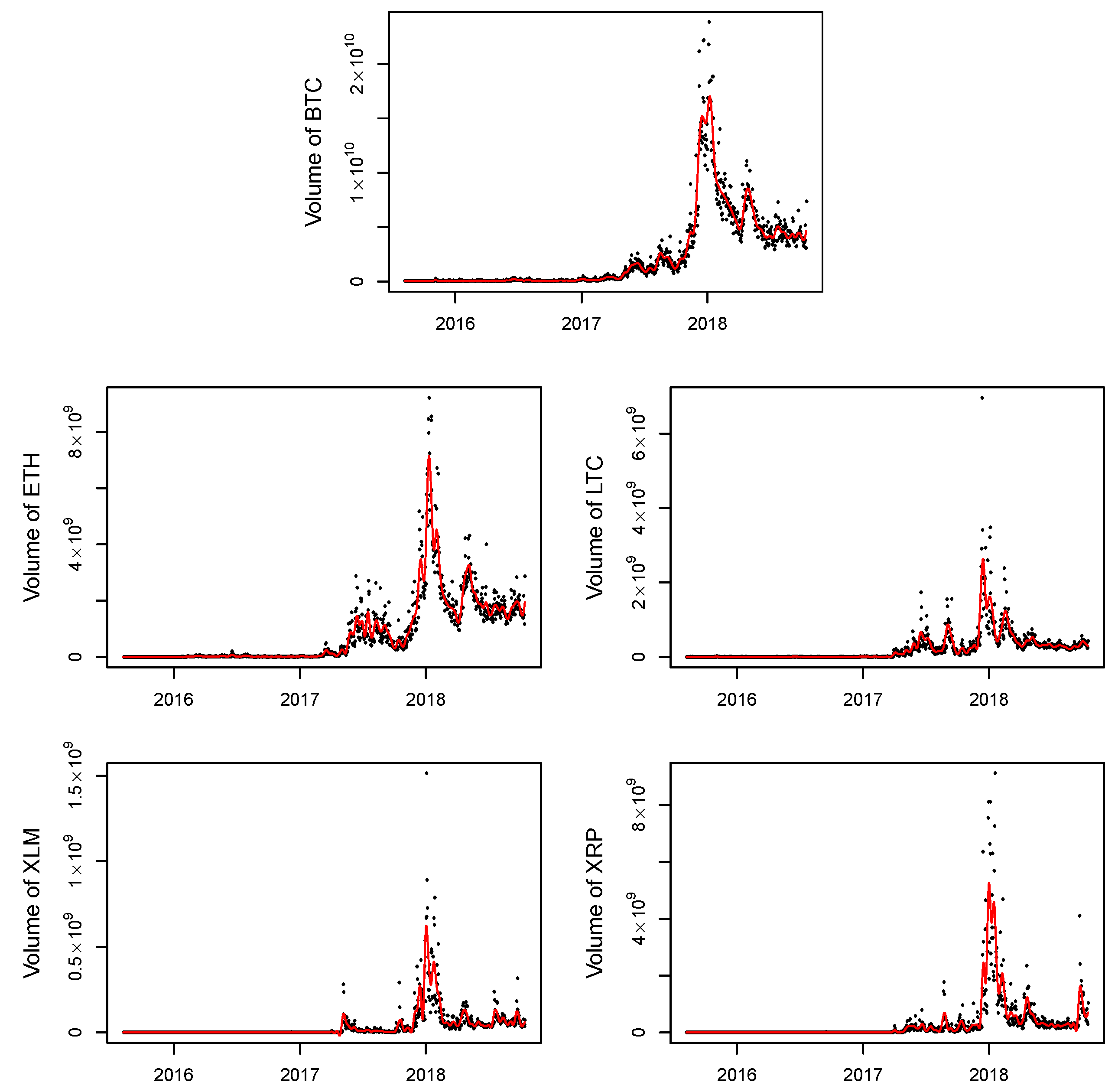
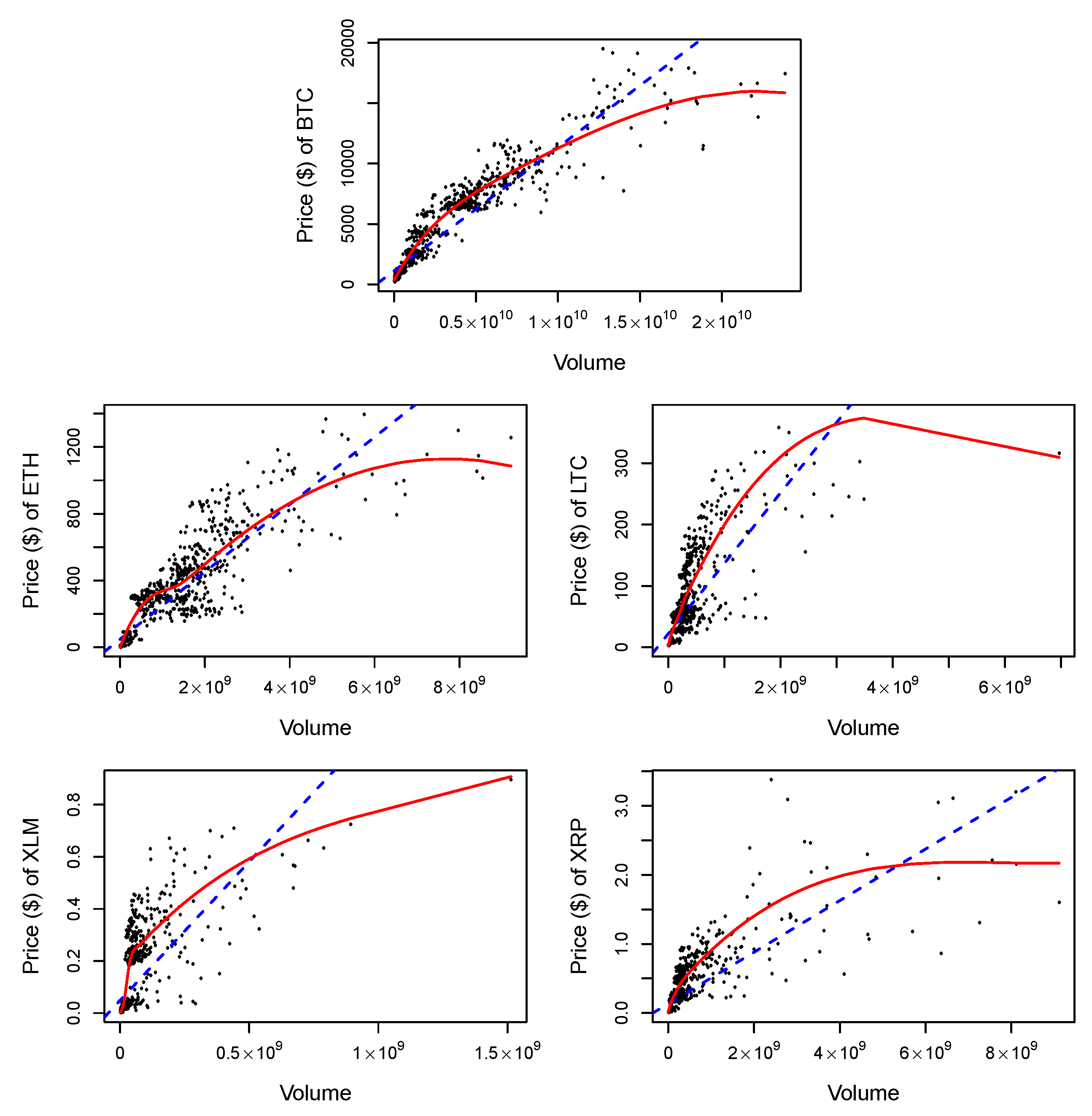
Finally, it seems natural to study trading volume in the market. We examine the volumes of the five cryptocurrencies. Table 5 provides descriptive statistics for the volumes of the five cryptocurrencies. We fit smoothing splines to the data in Figure 4. The study of the relationship between price and volume is also important because both daily price and volume data are generally available, and these data provide valuable information about future market movements since volume is deemed to lead the trend of prices. In Figure 5, we present linear and LOESS regression fits to the data. The estimated correlation coefficient and determination of coefficient are presented in Table 6 with the pseudo value defined by the squared correlation between the observed price values and the fitted values.
As illustrated in Figure 5, nonlinear fits (LOESS) between prices and volumes (in $) show better fitness compared to the linear regression models. These findings are supported by higher values of pseudo of LOESS fits compared to of the linear models in Table 6. Bitcoin shows the highest while the volatility of Ripple prices is least explained by trading volumes (in $), which is also addressed in Figure 5.
4. Discussion
Understanding the dependence structures among cryptocurrencies is important to both investors and policymakers. In this paper, we discuss the directional dependency of five cryptocurrencies by using the bivariate Gaussian copula beta regression with the neural network model for marginal distribution. To the best of our knowledge, our paper is the first study to analyze directional dependence among cryptocurrencies using neural networks autoregression and copular regression models. We argue that the proposed methods allow us to deal with problems by violations of traditional model assumptions in financial data analysis and are even superior to other remedies introduced in the literature. Using the daily log-returns, the major finding of our analysis is that, overall, directional dependence among the five cryptocurrencies exists and the return shocks of Bitcoin have the most effect on Litecoin. In addition, Stellar has relatively stronger impact on Ripple and the return shocks of Ethereum relatively influence the shocks of the other four cryptocurrencies instead of being influenced by them. This finding is somewhat opposed to the public perception that Bitcoin has consistently been leading and influencing all other cryptocurrencies (per se Altcoins) including Ethereum. Based on what we found, however, at least during our sample period, Ethereum has more influence on the other four cryptocurrencies rather than being impacted by them.
In recent literature, Ziȩba et al. (2019) examined interdependencies between log-returns of cryptocurrencies applying the two-step analysis, minimum spanning tree method and vector autoregression model. They found that, despite Bitcoin’s dominance in the market, changes in Bitcoin price do not affect and are not affected by changes in prices of other cryptocurrencies. The most influential ones are Litecoin and Dogecoin. They, however, indicate that findings obtained for Bitcoin shall not be generalized to the entire cryptocurrency market. Ji et al. (2019) studied a set of measures developed by Diebold and Yilmaz (2012, 2016) to examine returns-connectedness and volatility-connectedness networks among six large cryptocurrencies. The results show that Litecoin plays a central role of return and volatility connectedness instead of the largest cryptocurrency, Bitcoin. They suggested that this finding is evidence that the dominance of Bitcoin in the cryptocurrency market has been weakened. Bouri et al. (2019c) also examined the linkages among the volatility surprises of eight large cryptocurrencies (Bitcoin, Ethereum, Litecoin, Ripple, Stellar, Monero, Nem, and Dash) via the Granger-causality in the frequency-domain of Breitung and Candelon (2006). They showed that Bitcoin does not necessarily cause volatility surprises of the other cryptocurrencies and some cryptocurrencies (Stellar and Dash) show relatively independent price volatility.
These findings go along with our results where the Bitcoin has weakened its dominance in the crypto world and the market structure has been evolved rapidly. Some results, however, do not concord with our findings in part. One plausible explanation is that this could come from either still not sufficient knowledge on cryptocurrencies or different statistical procedures and analytical methods. It would be worthwhile to compare our findings from these studies. We claim, however, that these contradictory results also address the dynamic market structure in the cryptocurrency market. These areas will be addressed in future phases of this project.
Cryptocurrencies are still new to the public but have gradually captured its attention. The techniques we use in the paper may prove useful to others interested in examining the dependence relationships among cryptocurrencies. Our findings can assist crypto-investors by providing the directional dependence among major cryptocurrencies. This allows the investors to build the market-timing strategies by observing the directional flow of return shocks among cryptocurrencies. In addition, by addressing how significantly the return shock of one cryptocurrency influences one another, investors may improve their portfolio diversification.
Author Contributions
Conceptualization, J.L., S.H.,and J.-M.K.; methodology, J.-M.K.; software, S.H. and J.-M.K.; validation, S.H. and J.-M.K.; formal analysis, S.H. and J.-M.K.; investigation, J.L. and C.J.; resources, J.L. and J.-M.K.; data curation, S.H. and J.K.; writing—original draft preparation, J.L., S.H., and J.-M.K.; writing—review and editing, S.H., J.-M.K., and C.J.; visualization, S.H.; supervision, C.J.; project administration, C.J.; and funding acquisition, C.J.
Funding
This research received no external funding.
Acknowledgments
We are thankful to two anonymous referees for their meaningful comments and constructive suggestions that have improved the paper.
Conflicts of Interest
The authors declare no conflict of interest.
References
- Azoff, E. Michael. 1994. Neural Network Time Series Forecasting of Financial Markets. New York: John Wiley and Sons. [Google Scholar]
- Bação, Pedro, António Duarte, Helder Sebastião, and Srdjan Redzepagic. 2018. Information Transmission Between Cryptocurrencies: Does Bitcoin Rule the Cryptocurrency World? Scientific Annals of Economics and Business 65: 97–117. [Google Scholar] [CrossRef]
- Bouri, Elie, Syed Jawad Hussain Shahzad, and David Roubaud. 2019a. Co-explosivity in the cryptocurrency market. Finance Research Letters 29: 178–83. [Google Scholar] [CrossRef]
- Bouri, Elie, Rangan Gupta, and David Roubaud. 2019b. Herding behaviour in cryptocurrencies. Finance Research Letters 29: 216–21. [Google Scholar] [CrossRef]
- Bouri, Elie, Brian Lucey, and David Roubaud. 2019c. The volatility surprise of leading cryptocurrencies: Transitory and permanent linkages. Finance Research Letters. [Google Scholar] [CrossRef]
- Breitung, Jörg, and Bertrand Candelon. 2006. Testing for short-and long-run causality: A frequency-domain approach. Journal of Econometrics 132: 363–78. [Google Scholar] [CrossRef]
- Chang, Eric C., Joseph W. Cheng, and Ajay Khorana. 2000. An examination of herd behaviour in equity markets: An international perspective. Journal of Banking & Finance 24: 1651–99. [Google Scholar]
- Cherubini, Umberto, Fabio Gobbi, Sabrina Mulinacci, and Silvia Romagnoli. 2011. Dynamic Copula Methods in Finance, 1st ed. New York: John Wiley and Sons. [Google Scholar]
- Corbet, Shaen, Andrew Meegan, Charles Larkin, Brian Lucey, and Larisa Yarovaya. 2018. Exploring the dynamic relationships between cryptocurrencies and other financial assets. Economics Letters 165: 28–34. [Google Scholar] [CrossRef]
- Diebold, Francis X., and Kamil Yilmaz. 2012. Better to give than to receive: Predictive directional measurement of volatility spillovers. International Journal of Forecasting 28: 57–66. [Google Scholar] [CrossRef]
- Diebold, Francis X., and Kamil Yilmaz. 2016. Trans-Atlantic equity volatility connectedness: U.S. and European financial institutions, 2004–2014. Journal of Financial Econometrics 14: 81–127. [Google Scholar] [CrossRef]
- Dyhrberg, Anne Haubo. 2016. Bitcoin, gold and the dollar-A GARCH volatility analysis. Financial Research Letters 16: 85–92. [Google Scholar] [CrossRef]
- Faraway, Julian, and Chris Chatfield. 1998. Time series forecasting with neural networks: A comparative study using the airline data. Applied Statistics 47: 231–50. [Google Scholar] [CrossRef]
- Ferrari, Silvia, and Francisco Cribari-Neto. 2004. Beta regression for modelling rates and proportions. Journal of Applied Statistics 31: 799–815. [Google Scholar] [CrossRef]
- Gkillas, Konstantinos, and Paraskevi Katsiampa. 2018. An Application of Extreme Value Theory to Cryptocurrencies. Economics Letters 164: 109–11. [Google Scholar] [CrossRef]
- Masarotto, Guido, and Cristiano Varin. 2017. Gaussian Copula Regression in R. Journal of Statistical Software 77: 1–26. [Google Scholar] [CrossRef]
- Guolo, Annamaria, and Cristiano Varin. 2014. Beta regression for time series analysis of bounded data, with application to Canada Google Flu Trends. The Annals of Applied Statistics 8: 74–88. [Google Scholar] [CrossRef]
- Hencic, Andrew, and Christian Gouriéroux. 2015. Noncausal Autoregressive Model in Application to Bitcoin/USD Exchange Rate. In Econometrics of Risk. Studies in computational intelligence. Cham: Springer, vol. 583, pp. 17–40. [Google Scholar]
- Hertz, John, Anders Krogh, and Richard Palmer. 1991. Introduction to the Theory of Neural Computation. Redwood City: Addison-Wesley. [Google Scholar]
- Hyndman, Rob, George Athanasopoulos, Chrisoph Bergmeir, Gabriel Caceres, Leanne Chhay, Mitchell O’Hara-Wild, Fotios Petropoulos, Slava Razbash, Earo Wang, and Farah Yasmeen. 2019. Forecast: Forecasting Functions for Time Series and Linear Models, R Package Version 8.8; Available online: http://pkg.robjhyndman.com/forecast (accessed on 5 August 2019).
- Ji, Qiang, Elie Bouri, Chi Keung Lau, and David Roubaud. 2019. Dynamic connectedness and integration in cryptocurrency markets. International Review of Financial Analysis 63: 257–72. [Google Scholar] [CrossRef]
- Jondeau, Eric, and Michael Rockinger. 2006. The copula-garch model of conditional dependencies: An international stock market application. Journal of International Money and Finance 25: 827–53. [Google Scholar] [CrossRef]
- Katsiampa, Paraskevi. 2017. Volatility estimation for Bitcoin: A comparison of GARCH models. Economics Letters 158: 3–6. [Google Scholar] [CrossRef] [Green Version]
- Katsiampa, Paraskevi. 2019. An empirical investigation of volatility dynamics in the cryptocurrency market. Research in International Business and Finance 50: 322–35. [Google Scholar] [CrossRef]
- Kim, Jong-Min, and Sun-Young Hwang. 2017. Directional Dependence via Gaussian Copula Beta Regression Model with Asymmetric GARCH Marginals. Communications in Statistics: Simulation and Computation 46: 7639–53. [Google Scholar] [CrossRef]
- Kojadinovic, Ivan, and Jun Yan. 2010. Modeling multivariate distributions with continuous margins using the copula R package. Journal of Statistical Software 34: 1–20. [Google Scholar] [CrossRef]
- Kristoufek, Ladislav. 2013. Bitcoin meets Google Trends and Wikipedia: Quantifying the relationship between phenomena of the Internet era. Scientific Reports 3: 3415. [Google Scholar] [CrossRef]
- Kuan, Chung-Ming, and Halbert White. 1994. Artificial neural networks: An econometric perspective (with discussion). Econometric Reviews 13: 1–143. [Google Scholar] [CrossRef]
- Masarotto, Guido, and Cristiano Varin. 2012. Gaussian copula marginal regression. Electronic Journal of Statistics 6: 1517–49. [Google Scholar] [CrossRef]
- Nelsen, Roger B. 2006. An Introduction to Copulas, 2nd ed. New York: Springer. [Google Scholar]
- Phillips, Peter, Shuping Shi, and Jun Yu. 2015. Testing for multiple bubbles: Historical episodes of exuberance and collapse in the S&P 500. International Economic Review 56: 1043–78. [Google Scholar]
- Ripley, Brian D. 1996. Pattern Recognition and Neural Networks. Cambridge: Cambridge University Press. [Google Scholar]
- Sklar, Abe. 1973. Random variables, joint distribution functions, and copulas. Kybernetika 9: 449–60. [Google Scholar]
- Stavroyiannis, Stavros, and Vassilios Babalos. 2017. Herding, faith-based investments and the global financial crisis: Empirical evidence from static and dynamic models. Journal of Behavioral Finance 18: 478–489. [Google Scholar] [CrossRef]
- Sungur, Engin A. 2005. A note on directional dependence in regression setting. Communications in Statistics: Theory and Methods 34: 1957–65. [Google Scholar] [CrossRef]
- Ziȩba, Damian, Ryszard Kokoszczyński, and Katarzyyna Śledziewska. 2019. Shock transmission in the cryptocurrency market. Is Bitcoin the most influential? International Review of Financial Analysis 64: 102–25. [Google Scholar] [CrossRef]
Figure 1.
Prices of the five cryptocurrencies from 8 August 2015 to 15 October 2018.

Figure 2.
Residuals from neural network autoregression NNAR models to the daily log-returns in percentage of the five cryptocurrencies.
Figure 2.
Residuals from neural network autoregression NNAR models to the daily log-returns in percentage of the five cryptocurrencies.

Figure 3.
Copula directional dependence among the five cryptocurrencies. The thickness of the arrows reflects the strength of copula directional dependence, with thicker arrows indicating stronger pairwise directional dependence.
Figure 3.
Copula directional dependence among the five cryptocurrencies. The thickness of the arrows reflects the strength of copula directional dependence, with thicker arrows indicating stronger pairwise directional dependence.

Figure 4.
Smoothing spline fit to the volumes of the five cryptocurrencies.

Figure 5.
Linear and LOESS regression models between prices and volumes of the five cryptocurrencies: linear fit (dashed line) and LOESS fit (solid line).
Figure 5.
Linear and LOESS regression models between prices and volumes of the five cryptocurrencies: linear fit (dashed line) and LOESS fit (solid line).


Table 1.
Descriptive statistics of the five cryptocurrencies. The sample consists of 1165 daily log-returns of the five cryptocurrencies from 8 August 2015 to 15 October 2018.
Table 1.
Descriptive statistics of the five cryptocurrencies. The sample consists of 1165 daily log-returns of the five cryptocurrencies from 8 August 2015 to 15 October 2018.
| LBTC | LETH | LLTC | LXLM | LXRP | |
|---|---|---|---|---|---|
| Minimum | −20.7530 | −31.5469 | −39.5151 | −36.6358 | −61.6273 |
| Q1 | −0.9719 | −2.6806 | −1.6928 | −3.2394 | −2.1367 |
| Q2 | 0.2967 | −0.0894 | 0.0000 | −0.4066 | −0.3564 |
| Mean | 0.2775 | 0.4836 | 0.2283 | 0.3886 | 0.3407 |
| Q3 | 1.8199 | 3.2674 | 1.7673 | 3.1298 | 1.8960 |
| Maximum | 22.5119 | 41.2337 | 51.0348 | 72.3102 | 102.7356 |
| Skewness | −0.2519 | 0.5072 | 1.3240 | 2.0427 | 2.9787 |
| Kurtosis | 7.9613 | 7.6037 | 16.1616 | 18.0902 | 40.6386 |
Table 2.
Correlation coefficients, r and the coefficients of determination, . This table presents the Pearson’s correlation coefficients and the coefficients of determination of log-returns of the five cryptocurrencies.
Table 2.
Correlation coefficients, r and the coefficients of determination, . This table presents the Pearson’s correlation coefficients and the coefficients of determination of log-returns of the five cryptocurrencies.
| r | |||||||||
|---|---|---|---|---|---|---|---|---|---|
| LETH | LLTC | LXLM | LXRP | LETH | LLTC | LXLM | LXRP | ||
| LBTC | 0.369 | 0.591 | 0.342 | 0.285 | LBTC | 0.136 | 0.350 | 0.117 | 0.081 |
| LETH | 0.359 | 0.257 | 0.239 | LETH | 0.129 | 0.066 | 0.057 | ||
| LLTC | 0.366 | 0.345 | LLTC | 0.134 | 0.119 | ||||
| LXLM | 0.540 | LXLM | 0.292 | ||||||
Table 3.
The Optimal model structure using neural networks autoregression models, . This table shows the optimal model structure of estimating nonlinear autocorrelations in log-returns of five cryptocurrencies. The p and k represent the lags and hidden nodes, respectively, used in the model.
Table 3.
The Optimal model structure using neural networks autoregression models, . This table shows the optimal model structure of estimating nonlinear autocorrelations in log-returns of five cryptocurrencies. The p and k represent the lags and hidden nodes, respectively, used in the model.
| LBTC | LETH | LLTC | LXLM | LXRP |
|---|---|---|---|---|
| NNAR(1,1) | NNAR(4,2) | NNAR(8,4) | NNAR(9,5) | NNAR(18,10) |
Table 4.
The results of copula directional dependence. The higher value of copula directional dependence between each direction is highlighted in bold.
Table 4.
The results of copula directional dependence. The higher value of copula directional dependence between each direction is highlighted in bold.
| (U,V) | V → U | U→ V | Diff = (V→ U - U→ V) | ||||
|---|---|---|---|---|---|---|---|
| Estimate (Diff) | Bias (Diff) | Std. Error (Diff) | MSE (Diff) | Boot 95% CI of Diff | |||
| (LBTC, LETH) | 0.1325 | 0.1028 | 0.0295 | 0.000002 | 0.000175 | 0.00000003 | (0.0291, 0.0298) |
| (LBTC, LLTC) | 0.3852 | 0.3890 | −0.0037 | 0.000003 | 0.000360 | 0.00000013 | (−0.0044, −0.0030) |
| (LBTC, LXLM) | 0.1299 | 0.1159 | 0.0143 | 0.000001 | 0.000180 | 0.00000003 | (0.0139, 0.0146) |
| (LBTC, LXRP) | 0.1141 | 0.1006 | 0.0138 | 0.000004 | 0.000186 | 0.00000003 | (0.0134, 0.0142) |
| (LETH, LLTC) | 0.1240 | 0.1578 | −0.0333 | 0.000007 | 0.000197 | 0.00000004 | (−0.0337, −0.0329) |
| (LETH, LXLM) | 0.1016 | 0.1090 | −0.0075 | −0.000003 | 0.000161 | 0.00000003 | (−0.0078, −0.0072) |
| (LETH, LXRP) | 0.0893 | 0.0974 | −0.0082 | −0.000002 | 0.000160 | 0.00000003 | (−0.0085, −0.0079) |
| (LLTC, LXLM) | 0.1863 | 0.1611 | 0.0250 | −0.000001 | 0.000219 | 0.00000005 | (0.0246, 0.0255) |
| (LLTC, LXRP) | 0.1587 | 0.1450 | 0.0134 | −0.000006 | 0.000224 | 0.00000005 | (0.0129, 0.0138) |
| (LXLM, LXRP) | 0.2111 | 0.2208 | −0.0093 | 0.000004 | 0.000208 | 0.00000004 | (−0.0097, −0.0089) |
Table 5.
Summary statistics of the volumes of the five cryptocurrencies. Daily trading volumes (in $) of Bitcoin (BTC), Ethereum (ETH), Litecoin (LTC), Stella (XLM), and Ripple (XRP) are shown in the table.
Table 5.
Summary statistics of the volumes of the five cryptocurrencies. Daily trading volumes (in $) of Bitcoin (BTC), Ethereum (ETH), Litecoin (LTC), Stella (XLM), and Ripple (XRP) are shown in the table.
| BTC | ETH | LTC | XLM | XRP | |
|---|---|---|---|---|---|
| Minimum | 12,712,600 | 102,128 | 507,480 | 491 | 24,819 |
| Q1 | 68,338,000 | 8,933,050 | 2,374,230 | 31,416 | 722,260 |
| Q2 | 277,084,992 | 69,245,600 | 12,755,200 | 543,934 | 5,013,190 |
| Mean | 2,347,742,132 | 821,315,142 | 224,843,171 | 37,125,273 | 307,798,172 |
| Q3 | 3,961,080,064 | 1,475,939,968 | 302,471,008 | 40,041,100 | 249,264,000 |
| Maximum | 23,840,899,072 | 9,214,950,400 | 6,961,679,872 | 1,513,270,016 | 9,110,439,936 |
Table 6.
Pearson’s correlation coefficient r, determination of coefficients of linear regression models between prices and volumes, and pseudo values from LOESS fit are provided in the table.
Table 6.
Pearson’s correlation coefficient r, determination of coefficients of linear regression models between prices and volumes, and pseudo values from LOESS fit are provided in the table.
| BTC | ETH | LTC | XLM | XRP | |
|---|---|---|---|---|---|
| r | 0.937 | 0.893 | 0.763 | 0.706 | 0.778 |
| 0.879 | 0.797 | 0.582 | 0.499 | 0.606 | |
| 0.950 | 0.862 | 0.757 | 0.774 | 0.778 |
© 2019 by the authors. Licensee MDPI, Basel, Switzerland. This article is an open access article distributed under the terms and conditions of the Creative Commons Attribution (CC BY) license (http://creativecommons.org/licenses/by/4.0/).
Share and Cite
MDPI and ACS Style
Hyun, S.; Lee, J.; Kim, J.-M.; Jun, C. What Coins Lead in the Cryptocurrency Market: Using Copula and Neural Networks Models. J. Risk Financial Manag. 2019, 12, 132. https://doi.org/10.3390/jrfm12030132
AMA Style
Hyun S, Lee J, Kim J-M, Jun C. What Coins Lead in the Cryptocurrency Market: Using Copula and Neural Networks Models. Journal of Risk and Financial Management. 2019; 12(3):132. https://doi.org/10.3390/jrfm12030132
Chicago/Turabian StyleHyun, Steve, Jimin Lee, Jong-Min Kim, and Chulhee Jun. 2019. "What Coins Lead in the Cryptocurrency Market: Using Copula and Neural Networks Models" Journal of Risk and Financial Management 12, no. 3: 132. https://doi.org/10.3390/jrfm12030132