
Headland Rip Modelling at a Natural Beach under High-Energy Wave Conditions


CNRS, UMR 5805 EPOC, University of Bordeaux, 33615 Pessac, France
*
Author to whom correspondence should be addressed.
J. Mar. Sci. Eng. 2021, 9(11), 1161; https://doi.org/10.3390/jmse9111161
Submission received: 13 September 2021
/
Revised: 11 October 2021
/
Accepted: 15 October 2021
/
Published: 21 October 2021
(This article belongs to the Section Marine Energy)
Abstract
:A XBeach surfbeat model is used to explore the dynamics of natural headland rip circulation under a broad range of incident wave conditions and tide level. The model was calibrated and extensively validated against measurements collected in the vicinity of a 500-m rocky headland. Modelled bulk hydrodynamic quantities were in good agreement with measurements for two wave events during which deflection rips were captured. In particular, the model was able to reproduce the tidal modulation and very-low-frequency fluctuations (≈1 h period) of the deflection rip during the 4-m wave event. For that event, the synoptic flow behaviour shows the large spatial coverage of the rip which extended 1600 m offshore at low tide, when the surf zone limit extends beyond the headland tip. These results emphasize a deflection mechanism different from conceptualised deflection mechanisms based on the boundary length to surf zone width ratio. Further simulations indicate that the adjacent embayment is responsible for the seaward extent of the rip under energetic wave conditions. The present study shows that the circulation patterns along natural rugged coastlines are strongly controlled by the natural variability of the coastal morphology, including headland shape and adjacent embayments, which has implications on headland bypassing expressions.
1. Introduction
Rip currents are narrow and intense offshore-directed flows that can extend from the surf zone to potentially far seaward of the breaking point [1]. One of the main driving mechanisms for rip currents is alongshore variations in breaking wave heights [2]. These variations can be induced by different causes [3], which include alongshore variations of surf zone morphology (channel rips; e.g., [4]) or a shadowing effect due to the presence of a rigid boundary (shadow rips; e.g., [5]). Apart from alongshore variations in breaking wave heights, the deflection of a longshore current against a rigid boundary can also drive a rip current (deflection rips; e.g., [6]). Compared to transient hydrodynamically-controlled rips, bathymetrically-controlled and boundary-controlled rips are persistent in time and space. This makes them a critical component of the transport and the dispersion of sediments, pollutants or nutrients between the surf zone and the inner shelf along wave-exposed coasts. Channel rips have received much attention due to their ubiquity along open sandy beaches e.g., [7,8,9]. On the other hand, there is still a scarcity of studies along embayed beaches where boundary-controlled rips can potentially extend much further seaward than other types of rips [10].
Embayed beaches are ubiquitous along rugged coastlines where beaches are bounded by natural rocky headlands e.g., [11,12], and along artificial coastlines where man-made structures such as jetties or groynes are present e.g., [5,6]. Embayments may host a variety of circulation patterns depending on surf zone width and embayment length [13], as well as incident wave obliquity [14]. For obliquely incident waves, a prominent feature of coastal embayments is boundary-controlled rips, hereafter referred to as headland rips. Depending on the offshore wave obliquity with respect to the boundary, a headland deflection rip or a headland shadow rip flows against the boundary. Very few studies focusing on headland rips have been based on in-situ hydrodynamic measurements e.g., [5,6,15,16,17]. The field data-based studies of McCarroll et al. [16] and Scott et al. [6] have pointed out the large offshore extent of headland deflection rips along embayed beaches, compared to other types of rips (e.g., channel rips). For instance, McCarroll et al. [16] highlighted the presence of a deflection rip extending from two to three surf zone widths offshore under low-energy waves (with a significant wave height of 1 m) along a headland-bounded beach. For the same wave conditions, the authors showed that the shadow rip consisted of a closed circulation cell with low offshore exit rates. Their findings are in line with the modelling study along idealised embayed beaches of Castelle and Coco [10] who identified deflection rips as the main conduit for transporting floating materials offshore along wide embayments. For rips flowing against groynes, the experimental and modelling study of Scott et al. [6] emphasised the large offshore extent of deflection rips and pointed out the key role of the boundary length (distance from shoreline to boundary offshore tip) to surf zone width ratio in determining the circulation pattern. For a situation with a single groyne, the authors developed the following conceptualised deflection mechanism: the longshore current is fully transmitted to the other side of the boundary when < 0.5 (no deflection scenario), a part of the longshore current is deflected offshore while the other part is transmitted to the other side of the boundary when 0.5 < < 1.25, and the longshore current is fully deflected offshore by the boundary when > 1.25 (full deflection scenario). It should be noted that this deflection mechanism has been established for idealised boundaries with sharp and well-defined edges. Therefore, it must be validated with natural coasts where complex rocky headland morphologies and adjacent embayment geometry resulting from inherited geology may alter the traditional deflection pattern.
The field data-based studies to date have addressed the headland rip dynamics for low- to moderate-energy wave conditions (i.e., < 2 m) and for weakly-varying wave and tide conditions, thus preventing to frame an extensive synoptic view of these rips. In addition, the modulation of rip flows at the very-low-frequency time scale (VLF; period higher than tens of min) has been well investigated for channel rips along open sandy beaches e.g., [4], but has never been described for headland rips. Accordingly, the spatio-temporal variability of headland rips at a natural beach is poorly understood (e.g., magnitude, spatial scales, tidal and VLF modulation, response to varying incident wave conditions), in particular under high-energy obliquely-incident waves. Such understanding is crucial for better assessing sediment pathways along headlands and, in turn, evaluating embayment sediment budget. Indeed, few morphological studies suggest that headland rips can transport significant sediment quantities offshore [18] and to the adjacent embayment through headland sand bypassing mechanisms [17,19]. Headland rip channels can be sustained for long periods (e.g., several months; [20]), implying that headland rip flow may persistently transport sediment offshore. Headland deflection rips may provide sediment connections between adjacent embayments [21], and thus impact multi embayment-scale dynamics.
Overall, the headland deflection rip dynamics is still poorly understood and needs to be further addressed. With the aim of bridging such a knowledge gap, a three-week field experiment was conducted at La Petite Chambre d’Amour beach (PCA; Anglet, Southwest France) in October 2018 with the collection of an extensive dataset of waves and currents in the vicinity of a 500-m rocky headland [22]. Among the three main circulation configurations identified by Mouragues et al. [23], the deflection configuration featured an intense tidally-modulated rip flowing against the headland from the surf zone to far offshore, in particular during energetic wave conditions. For instance, under 4-m oblique waves, time- and depth-averaged velocities of the deflection rip reached up to 0.7 m/s 800-m offshore in 12-m depth. At that location, VLF fluctuations were remarkably energetic, increasing velocities up to two to three times their mean values. These measurements, which were limited in both time and space, suggest that the rip extended very far seaward of the headland tip.
Following the dataset analysis of Mouragues et al. [23], a coupled wave-circulation model is used to give a detailed and large-scale description of the nearshore circulation and also new insight into natural headland rip flow under a broad range of incident wave conditions and tide level. The goals are: (1) to frame a synoptic flow behaviour of the large-scale deflection rips; (2) to assess the validity of idealised deflection rip patterns for a natural beach with complex adjacent embayment and natural headland shape and (3) to explore the spatio-temporal variability of natural headland rips such as its VLF and tidal modulation along with its hydrodynamic response under a broad range of incident wave conditions.
2. Materials and Methods
2.1. Field Site and Experimental Dataset
From the 3 to the 26 of October 2018, a field experiment was conducted at La Petite Chambre d’Amour (PCA) beach located in Anglet along the Aquitaine south coast (SW France; Figure 1a). This rugged coast is a mesotidal high-energy environment that is regularly exposed to energetic Atlantic swells coming from the W-NW direction [24]. The average tidal range reaches 3.94 m for spring tides and 1.69 m for neap tides. PCA is a double-barred sandy beach located at the southern end of a 4-km embayment, comprising six groynes, bounded by the Adour dike to the North and by the Saint Martin 500-m rocky headland to the South (Figure 1b). The goal of the experiment was to study wave-induced circulation at a high-energy geologically-constrained beach. To do so, Acoustic Doppler Current Profilers (ADCPs; see SIG1, SIG2, SIG3 and AQ in Figure 1c) and surf-zone drifters were deployed to collect spatially dense and high-frequency Eulerian and Lagrangian velocity measurements. A more detailed description of the field site and the experiment can be found in Mouragues et al. [22], Mouragues et al. [23].
The dataset collected during two events for which a deflection rip was measured (hereafter referred to as deflection events) is used to calibrate and validate a coupled wave-circulation model. Both deflection events are presented in Section 2.2.2 while the model is described in the following section.
2.2. Numerical Modelling
2.2.1. XBeach Model
The open-source XBeach model (version 2015-10-22 v1.22.4867 Kingsday) is set up at PCA to investigate the deflection rip dynamics. XBeach is a morphodynamic model initially developed to reproduce storm response on sandy beaches where infragravity swash is dominant [25]. It solves the coupled two-dimensional horizontal (2DH) equations for wave propagation, flow, sediment transport and bottom changes. In this paper, the last two modules are disabled as only the deflection rip hydrodynamics is investigated. The so-called surfbeat approach (XB-SB) is used and resolves motions at the wave group (infragravity) scale while short waves are phase-averaged. This approach allows computing the low-frequency variability of hydrodynamic processes with a lower computational cost compared to the phase-resolving approach (see Appendix A for a brief description of the model). XB-SB is therefore suitable for modelling both the tidal modulation and VLF fluctuations of the deflection rip while being computationally efficient for large domains (>O(1) ) and events lasting several hours, as in the present study. XB-SB has been widely used to address bathymetrically-controlled rip currents along natural open sandy beaches e.g., [26] and boundary-controlled rips along artificial coastlines e.g., [6]. The surfbeat approach has also been found to correctly reproduce mean infragravity and VLF velocities along open rip-channelled beaches [27,28].
The XBeach model includes a number of free parameters that require to be calibrated with measurements. A prior sensitivity study was conducted to identify the hydrodynamic free parameters having the greatest impact on the deflection rip dynamics by comparing modelled and measured bulk hydrodynamic quantities (see Section 2.3). Two free parameters were chosen for further calibration: the breaking parameter controlling the surf zone width, and a bed friction Chezy coefficient C indirectly controlling the alongshore current magnitude. These two parameters were calibrated by minimizing, for both deflection events, residuals between the measured and modelled bulk quantities. Best agreements between the model and measurements were achieved with = 0.50 and C = 45 /s. Hereafter, these two parameters are set to their calibrated values while all other parameters are set to their default XBeach value. It should be noted that, in the present study, the viscosity was also set to its default XBeach value which is a constant value of 0.5 m/s. This sensitivity study included changing wave breaking and roller dissipation formulas and the associated free parameter values. The latter did not strongly altered model results.
2.2.2. Model Implementation
- Bathymetry
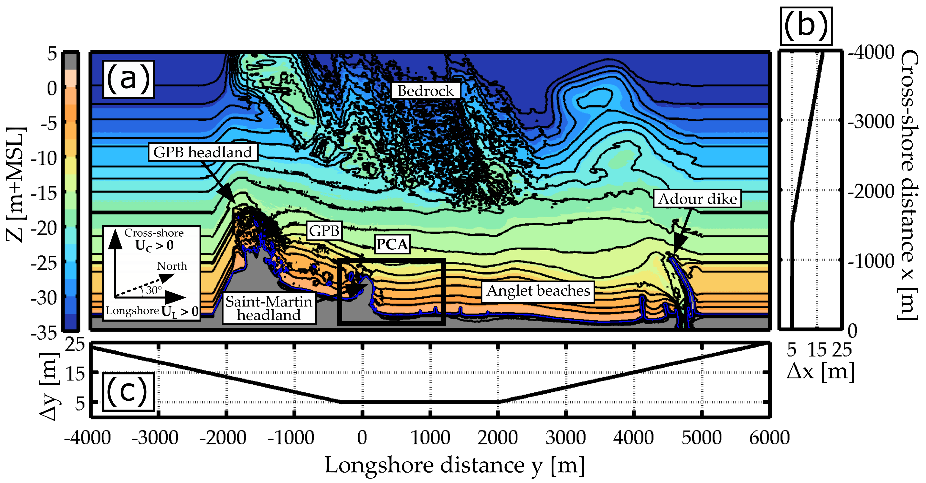
XB-SB was implemented on a regular grid rotated by to a local coordinate system extending 4000 m and 10,000 m in the cross-shore x and longshore y direction, respectively (Figure 2a). The computational domain comprises offshore small-scale bedrock and a sand deposit lobe (x < −2000 m) which play an important role in wave transformation [29,30]. Close to the shore, the domain comprises the Adour dike, the six groynes within Anglet beaches, the field site PCA and the Saint-Martin headland, the GPB adjacent embayment and its southern headland (GPB headland). Because the Anglet beach bathymetry was not available, the latter was manually filled by the alongshore-averaged cross-shore transect of PCA, from the southernmost groyne to the Adour dike (1000 m < y < 5000 m). To apply periodic conditions at the lateral boundaries and to avoid boundary effects under high-energy wave forcing, the bathymetry was extended in the longshore direction at both boundaries using an alongshore-averaged cross-shore transect from the northern part of the Adour dike. These lateral extensions were made large enough (2000 m and 1000 m at the southern and the northern boundary, respectively) to prevent side effects due to the presence of the GPB headland and the Adour dike. The mesh step size was set to 5 m at PCA, gradually increasing to 25 m close to the boundaries (Figure 2b,c).
- Modelled scenarios
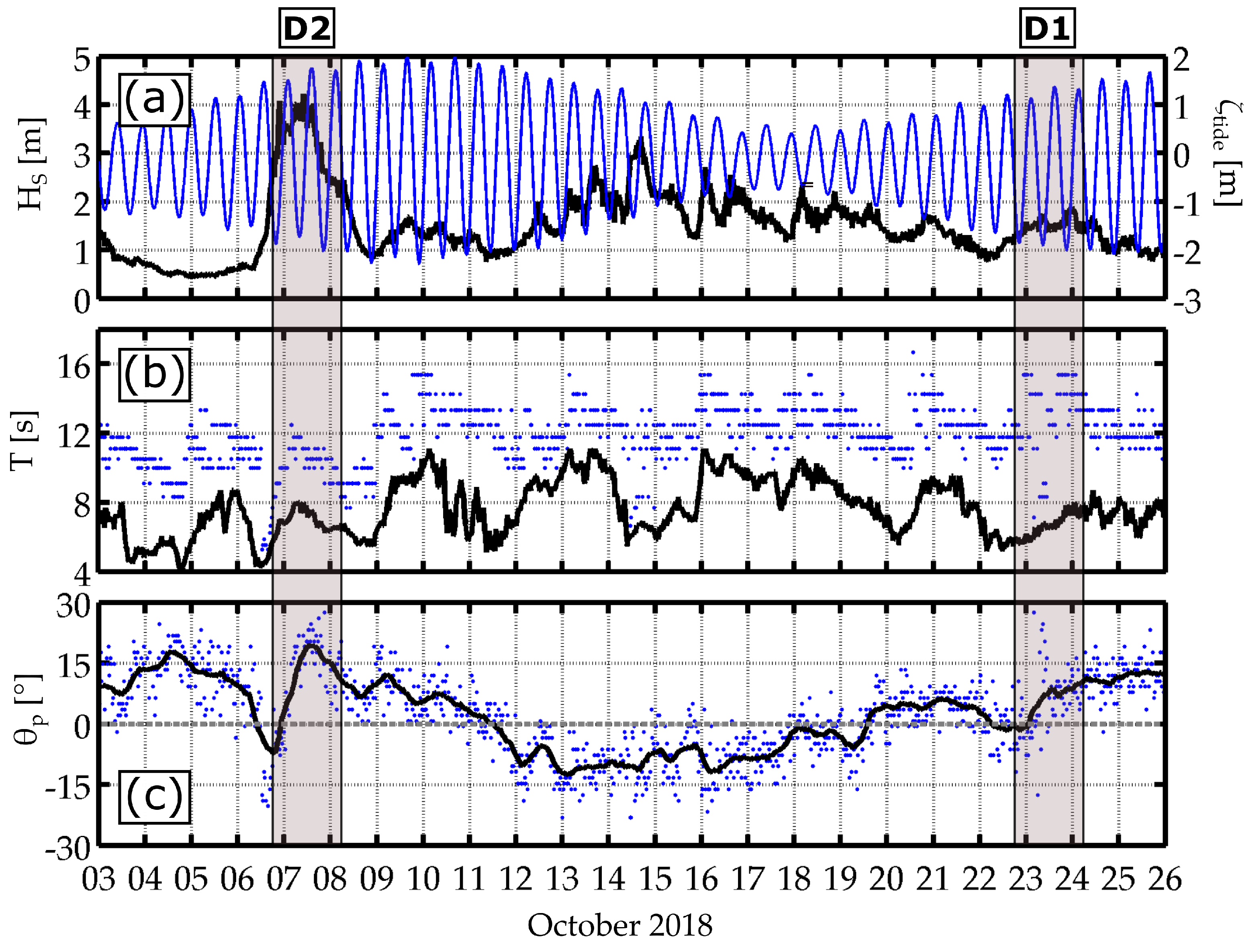
Modelled scenarios consist of two wave events for which a deflection rip was measured [23]. Both deflection events are characterized by different offshore wave conditions (hereafter, event D1 and D2 in Figure 3). During both events, the measured deflection rip flow was strongly modulated by the tide due to the control of tidal level on wave breaking patterns and also extended well beyond the surf zone. During event D1 ( m and ), the deflection rip extended at least 1000-m offshore in 14-m depth where mean Lagrangian surface velocities reached 0.3 m/s during the rising tide. During event D2 ( m and ), time- and depth-averaged Eulerian velocities displayed energetic VLF fluctuations, with periods of energy peaks of around 30 min and 1 h, increasing velocities up to 0.7 m/s at SIG1 located 800-m offshore in 12-m depth at low tide. At that same location, velocities decreased below 0.1 m/s around full high tide which indicated a strong tidal modulation. Events D1 and D2 are hereafter referred to as the low- and high-energy deflection event, respectively, and are used for the calibration and the validation of the model.
- Model forcing datasets
XB-SB was forced by the time-varying directional wave spectrum measured by a permanent directional wave buoy (Candhis buoy number 06402) moored in 50 m water depth and located along the open boundary x = −4000 m. The input wave spectrum is extrapolated to the entire open boundary. Based on the input wave spectrum, XB-SB uses a random phase summation procedure to reconstruct time series of short-wave energy varying at the wave-group scale, which were used to force the spectral wave model (see Appendix A).
The wave model is coupled, through a radiation stress gradients approach, with a circulation model which is forced by the incoming bound wave computed from Herbers et al. [31]. It should be noted that, due to the random phase summation procedure, times series of modelled infragravity surface elevation and velocities can vary between one simulation to another. To assess such variability, the model was run ten times using the same input spectrum but using ten different set of phases (i.e., ten different time series of short-wave energy and bound wave phases) which are randomly select by the model. Standard deviation of modelled outputs computed from these ten simulations was calculated for each simulated wave event (see Section 2.3).
Offshore wave spectrum and water level during events D1 and D2 are used to investigate the deflection rip dynamics (Figure 3). For model calibration and validation, the input water level corresponds to the time-varying tidal signal. In Section 3.4, the water level is kept constant to investigate the headland rip response to varying incident wave conditions. To avoid initial transient effects which, based on preliminary tests are less than 4 h, wave and current characteristics were computed over the last 28 h out of the total 32 h event duration. Because the wind speed during event D1 was low (<0.05 m/s; [23]), wind effects were not included in the event D1 modelling experiment. During event D2, the wind dataset was not available. For the latter high-energy event, wave breaking is the main driving mechanism for the nearshore circulation.
2.3. Bulk Hydrodynamic Quantities
To assess the model skill in reproducing the headland rip dynamics, the following wave and current bulk quantities were computed from the dataset (subscript M) and XBeach (subscript XB): the significant short wave height ( and ), the significant infragravity wave height ( and ) and time-averaged velocities.
Significant short and infragravity wave heights were calculated over 30-min bursts. For each burst, the measured significant wave heights were computed as four times the bandpass-filtered surface elevation standard deviation:
where and refer to the measured surface elevation that has been filtered within the gravity band (between and 0.5 Hz) and within the infragravity band (0.005 Hz and ), respectively. The split frequency is set to 60% of the peak frequency ( where is the peak frequency of the most offshore instrument). Note that surface elevation spectra of both events were qualitatively checked to ensure that corresponds to the frequency where energy between the gravity and infragravity band is minimum. The modelled significant wave heights were computed following [32]:
where corresponds to the 30-min time-averaging operator. is the modelled root-mean-square height computed as where is the instantaneous wave energy, the water density and g the gravitational constant. and are the modelled bandpass-filtered surface elevations, with similar gravity and infragravity frequency bands as for the measured wave heights.
Time-averaged velocities were defined as: 30 min-averaged Eulerian velocity magnitudes ( and ) to quantitatively assess the model skill in reproducing the tidal modulation of the rip flow and 5-min running-averaged Eulerian velocities (cross-shore and longshore) to look into the modulation of the rip at the VLF scale. Time-averaged Lagrangian velocities were also used to compare modelled mean velocity patterns with drifter measurements. To quantify the variability due to the random phase procedures, the time series of the standard deviation velocity resulting from the ten simulations was computed. A confidence interval of velocities was computed, with the upper (lower) limit of the confidence interval defined as the time series of the velocity from one individual simulation plus (minus) one standard deviation.
The correlation coefficient (), the root-mean-squared error (RMSE) and its normalized value (NRMSE) were used to quantitatively assess the model performance. The RMSE was computed as:
where X corresponds to one of the bulk hydrodynamic quantities. For (), the NRMSE corresponds to the RMSE divided by the average of all (). For , the NRMSE ocrresponds to the RMSE divided by the maximum of all . The latter definition prevents from obtaining biased errors when velocities are near zero.
3. Results
3.1. Model Assessment
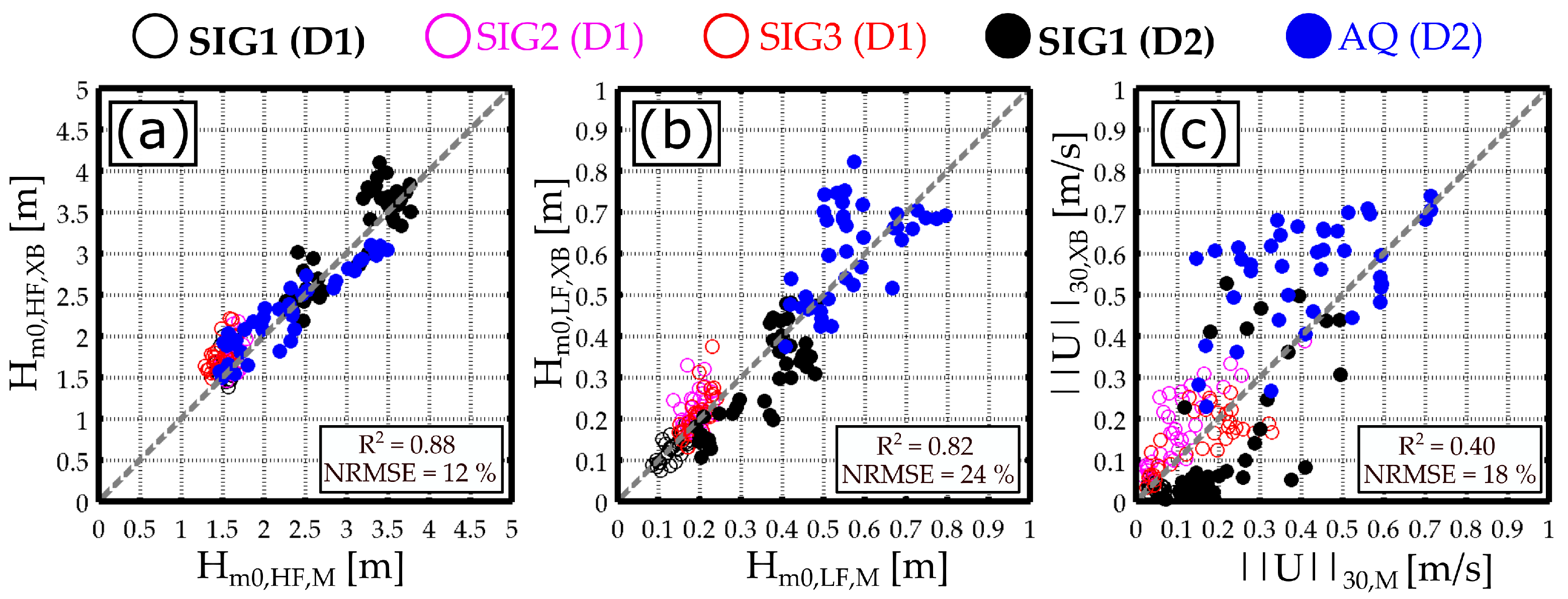
In this section, the calibrated model is compared against measurements for both deflection events. Figure 4 shows the measured and modelled significant short wave heights, significant infragravity wave heights and 30 min-averaged Eulerian velocity magnitudes for both events at each instrument location. Note that AQ was not measuring during event D1 while SIG2 and SIG3 were not measuring during event D2 [22]. Overall, both significant short and infragravity wave heights are well predicted by XB-SB with above 0.8 and relatively low RMSE (Figure 4a,b). XB-SB is also able to fairly well reproduce the mean Eulerian magnitude for both events ( = 0.40), with the same order of magnitude between the model and the dataset (NRMSE = 18%; Figure 4c).
Table 1 shows the RMSE and NRMSE of each bulk quantities, for each event and at each instrument location. It should be reminded that, for the sake of consistency, the model calibration was conducted to find a single couple of free parameters ( and C) fitting bulk quantities for both deflection events, as opposed to finding one couple of free parameters for one deflection event. This explains why some model performance statistics presented in Table 1 are only fair. For instance, errors can be relatively high (>20%) due to tidal modulation being slightly over- or under-estimated depending on deflection events. However, these errors are associated with low velocities. Overall, the model fairly reproduces all quantities considering the complexity of the study site which comprises headland, sandbars and rocky outcrops all affecting the nearshore circulation. To investigate the XB-SB ability to model both tidal and VLF modulations of deflection rips, the 5-min running-averaged Eulerian velocities at each ADCP location computed from the model are compared against the dataset for each event.
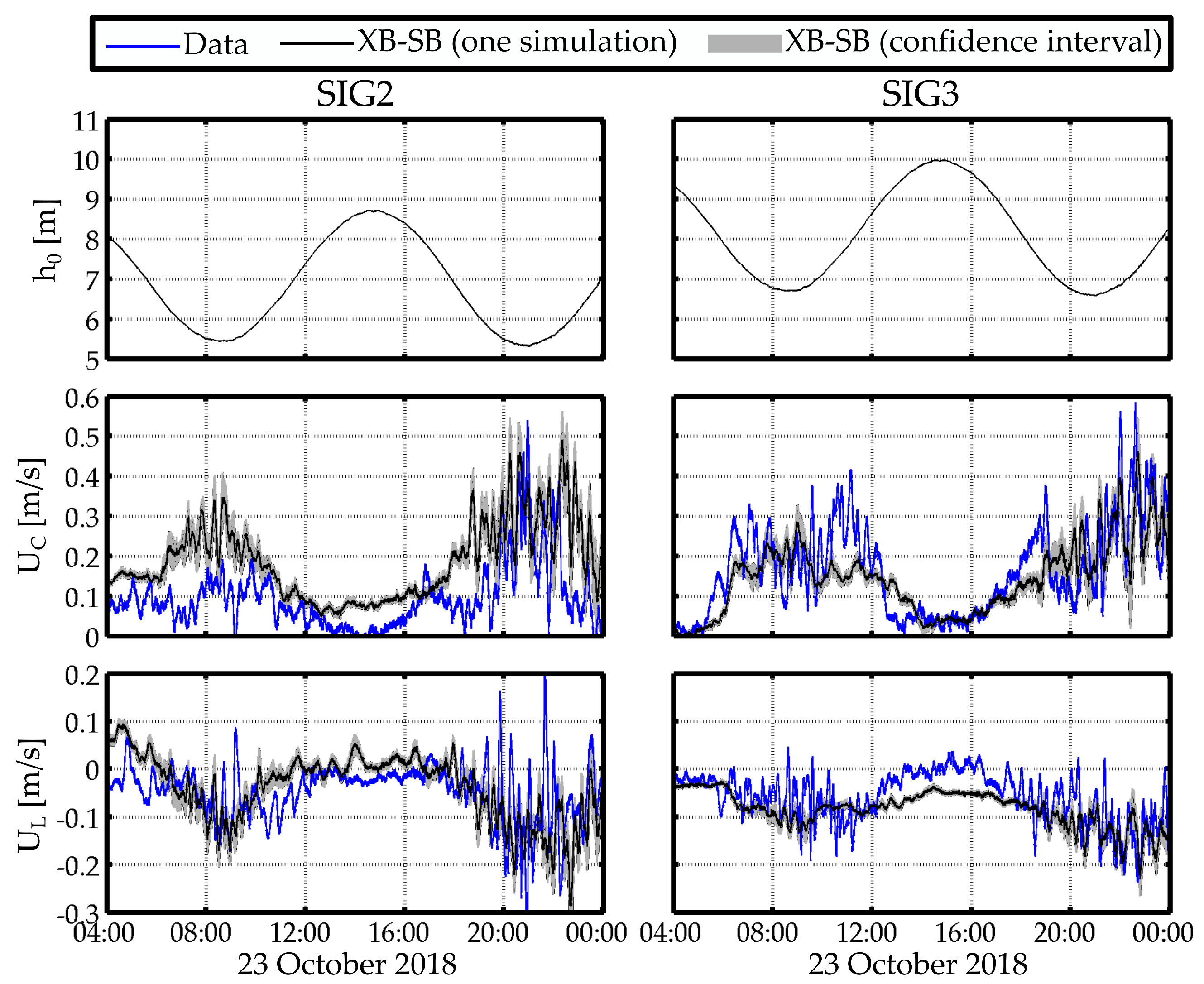
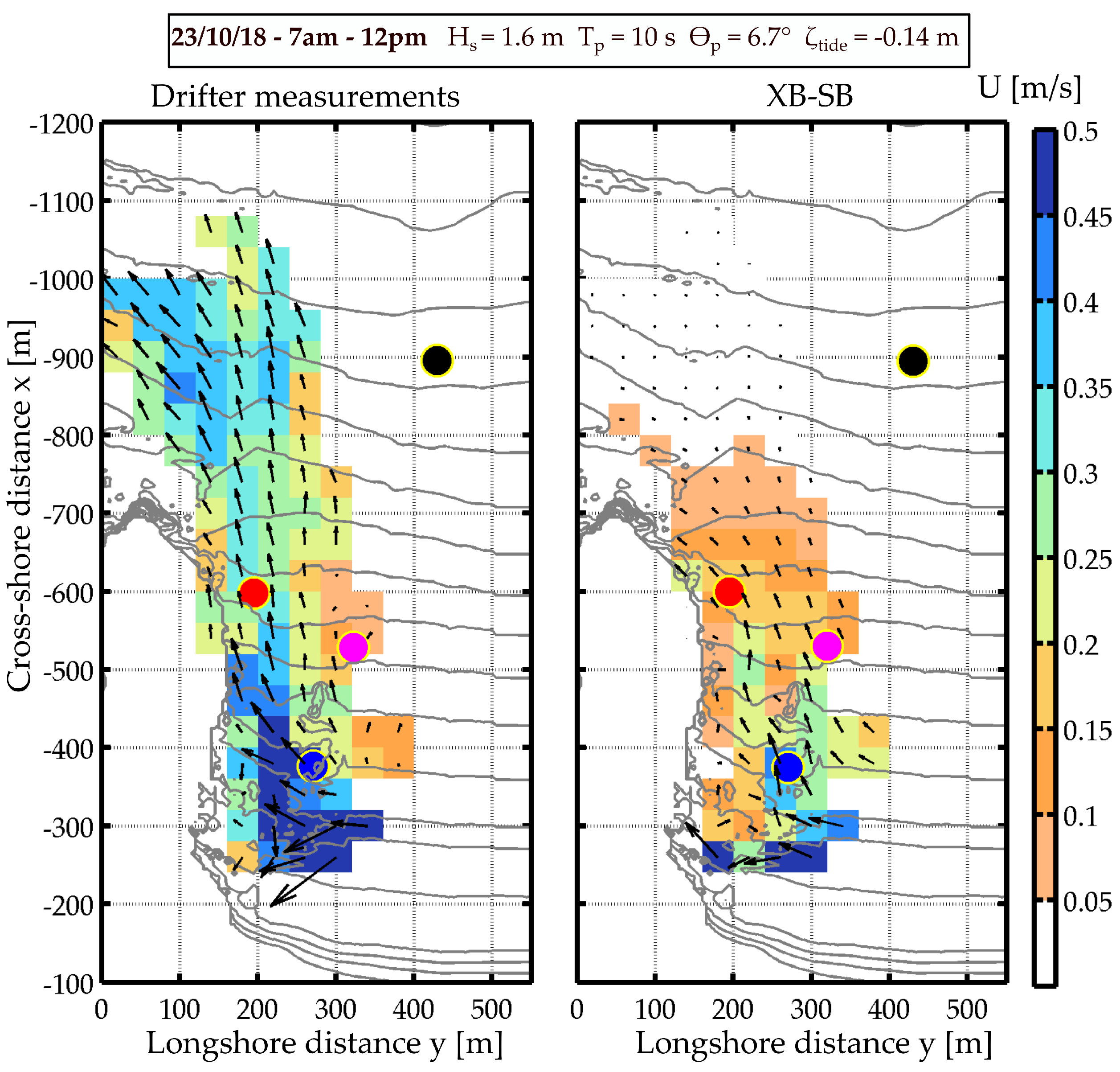
During event D1, both cross-shore and longshore velocity components of the deflection rip are fairly well predicted by the model (Figure 5). The model is able to reproduce the tidal modulation of the rip, with high velocities (>0.2 m/s) around low tide and near-zero velocities at high tide. At each instrument location, the confidence interval of velocity is relatively narrow suggesting that incident wave group and bound wave phases barely affect time series of the running-averaged velocities. During the first low tide, the cross-shore velocity at SIG2 is moderately overestimated by the model while the latter reproduces fairly well both velocity components at SIG3. This period corresponds to when surf-zone drifters were deployed close to the headland. This deployment allowed to map the measured mean Lagrangian surface currents (Figure 6a; [23]), emphasising the large spatial coverage of the deflection rip during the low-energy event. For the sake of model-data comparison, the mean Lagrangian depth-averaged currents modelled by XB-SB are interpolated onto the drifter spatial grid (Figure 6b). An analysis of the vertical variability of the flow has shown that the deflection rip flow measured at SIG2 and SIG3 was depth-uniform (not presented here). The drifter-derived surface currents are therefore representative of the flow inside the water column, at least onshore of SIG2 and SIG3 locations i.e., inside the surf zone and the deflection rip neck (x > −600 m). Within this area, the measured Lagrangian surface currents and the modelled Lagrangian depth-averaged currents are in good agreement, with both modelled and measured flow magnitude reaching around 0.2–0.3 m/s. Further offshore (inside the deflection rip head; x < −600 m), the flow magnitude predicted by the model is considerably underestimated. The modelled magnitude drops below 0.05 m/s 100 m seaward of the headland tip while the drifter surface magnitude reaches 0.4 m/s 300 m seaward of the tip. For such a low-energy deflection event, the model is therefore unable to reproduce the seaward extension of the rip, which will be discussed in Section 4.
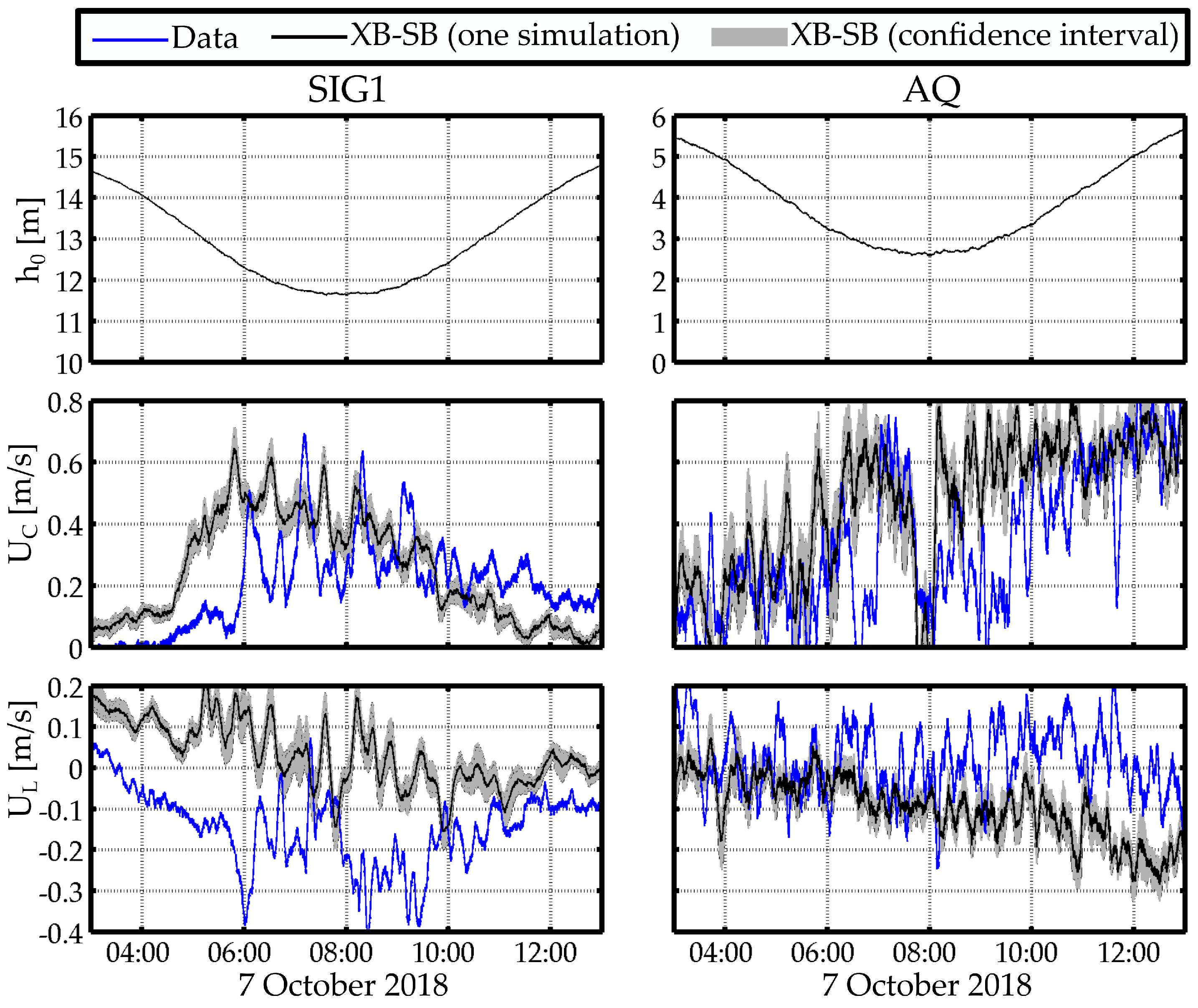
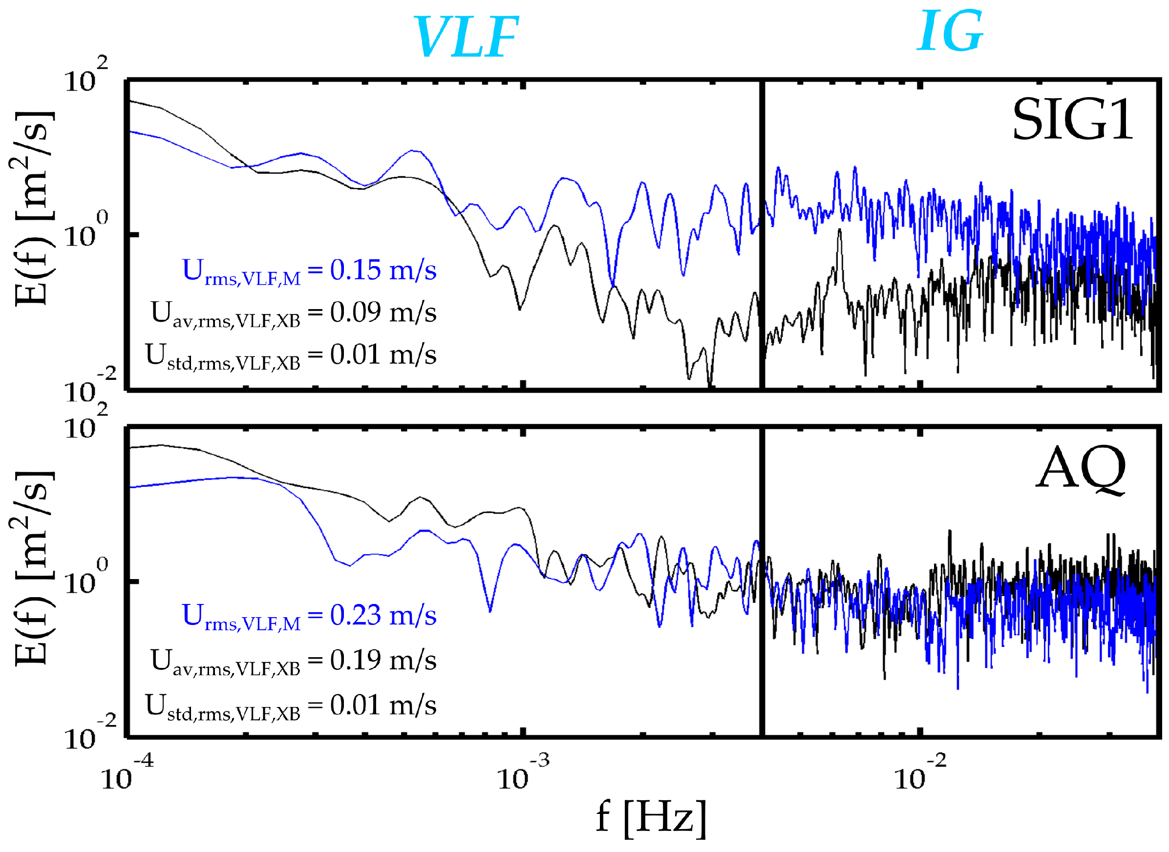
During event D2, modelled velocities of the deflection rip are in fair agreement with measurements, both inside the surf zone (AQ) and inside the rip head (SIG1; Figure 7). Well seaward of the outer edge of the surf zone, the strong tidal modulation is correctly reproduced by the model with intense velocities around low tide and near-zero velocities at high tide. Discrepancies between the model and measurements are however observed, such as the weak negative longshore current component at SIG1 which is not captured by the model. This indicates that the modelled rip head is directed offshore while the measured rip head is slightly directed toward the south. Lastly, while the modelled energy within the infragravity band is underestimated at SIG1, the energetic VLF fluctuations of the deflection rip are well computed by the model. Levels of energy and characteristic (peak) periods (order of 1 h and 30 min) of the measured and modelled VLF are of the same order (Figure 8). In line with the narrow confidence interval shown in Figure 7, the standard deviation of the root-mean-squared VLF magnitude computed from ten simulations is relatively low at both instrument locations (0.01 m/s; Figure 8).
Overall, the calibrated model is able to correctly reproduce wave and current characteristics as well as their tidal modulation for both deflection events. The energetic VLF fluctuations captured during the high-energy deflection event are also well computed by the model. During the low-energy deflection event, XB-SB is not able to reproduce the seaward extension of the rip.
3.2. Deflection Mechanism
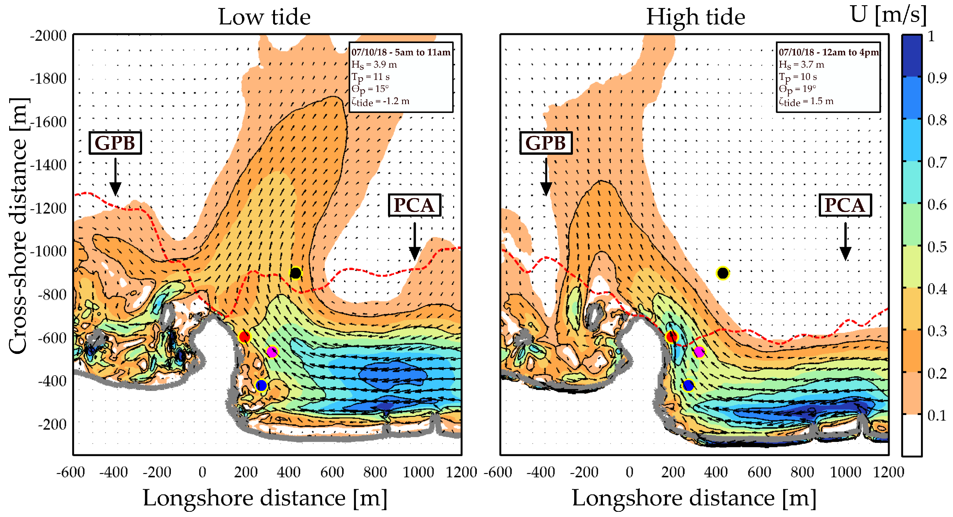
The model is now used to investigate the deflection rip flow pattern at PCA under high-energy wave conditions. Figure 9 shows the modelled velocity field averaged at low tide and high tide during event D2. These mean velocity patterns highlight the tidal modulation and the large spatial scales of the deflection rip at PCA. At low tide, the combination of a wide surf zone (≈600 m) and a strong longshore current (0.5–1.0 m/s) induces a wide deflection rip extending around 1600 m offshore in 19-m water depth where its magnitude reaches 0.2 m/s. Along the adjacent embayment (GPB), a longshore current is flowing towards PCA at low tide. This GPB current is 200-m wide and is relatively strong, with a magnitude reaching 0.–0.5 m/s. It contributes to the seaward deflection of the remaining portion of the PCA longshore current that is not deflected by the headland. This mechanism is ubiquitous at low tide when the surf zone extends beyond the headland tip ( < 1). At high tide ( > 1), the deflection rip and the surf zone are narrow and the PCA longshore current is fully deflected offshore against the headland. The GPB current is still intense but directed offshore which has a much weaker impact on the deflection pattern than at low tide.
These results emphasise a new deflection mechanism that is different from the previous mechanism conceptualised for rips flowing around groynes based on [6]. The circulation at PCA shows a full deflection scenario, regardless of . These results suggest that the adjacent embayment and, more generally, the prominent morphological features may exert significant control on the deflection rip pattern.
3.3. Morphological Control on Deflection Rip Pattern
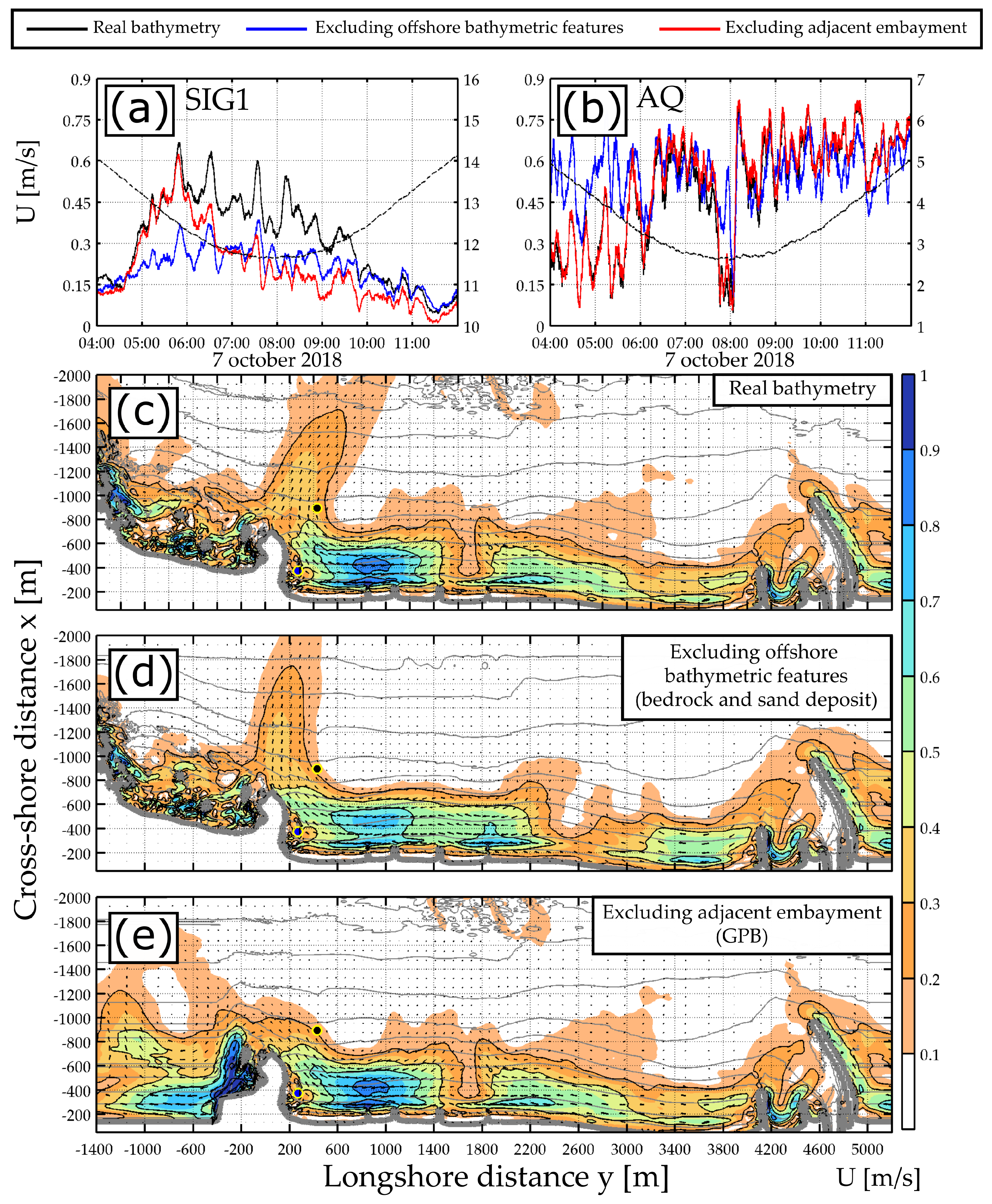
To assess the morphological control on the deflection pattern, the model is run on an idealised bathymetry excluding the most prominent morphological features of the field site. Four different idealised bathymetry scenarios are considered: (1) excluding the six groynes along Anglet beaches, (2) excluding both the groynes and the Adour dike, (3) excluding the offshore small-scale bedrock and sand deposit lobe (hereafter referred to as offshore bathymetric features) and (4) excluding the adjacent embayment. The model is forced by the same time series of short-wave energy and long-wave surface elevation at the offshore boundary as during event D2 to examine the potential effect of morphology on the very-low-frequency fluctuations which occurred at SIG1 and AQ. While idealised scenarios 1 and 2 do not affect the deflection rip dynamics (not presented here), the mean flow patterns are substantially altered in idealised scenarios 3 and 4.
The upper panels of Figure 10 show time series of the modelled velocity magnitude at SIG1 (a) and AQ (b) for the real bathymetry and for scenarios 3 and 4. The other panels show the large-scale modelled velocity field averaged at low tide for each considered scenario in the upper panels. Excluding the morphological features leads to a considerable drop of velocity magnitude at SIG1, as mean values are halved (Figure 10a). This is because SIG1 is nearly outside the deflection rip head for both idealised scenarios (Figure 10d,e). The presence of offshore bathymetric features leads to a significant longshore variability of the longshore current magnitude along Anglet beaches (at y ≈ 1600 m in Figure 10a). Such a variability is caused by the longshore variability of wave height and wave angle of incidence at breaking, enforced by wave refraction across the offshore bedrocks and sand deposit lobe (not shown here; in line with [29,30]). Excluding offshore bathymetric features leads to the smoothing of the longshore variability of the longshore current but does not significantly affect the deflection pattern. A change of the deflection rip head, becoming fully offshore-directed, is to be noted. On the other hand, excluding the adjacent embayment strongly alters the deflection pattern (Figure 10e). For such a scenario, the PCA longshore current is not deflected offshore and is transmitted to the other side of the headland, as anticipated by the conceptualised mechanism of [6] when < 1.25. These findings highlight the crucial role of the adjacent embayment in the full deflection scenario at PCA during event D2.
3.4. Headland Rip Response to Varying Incident Wave Conditions
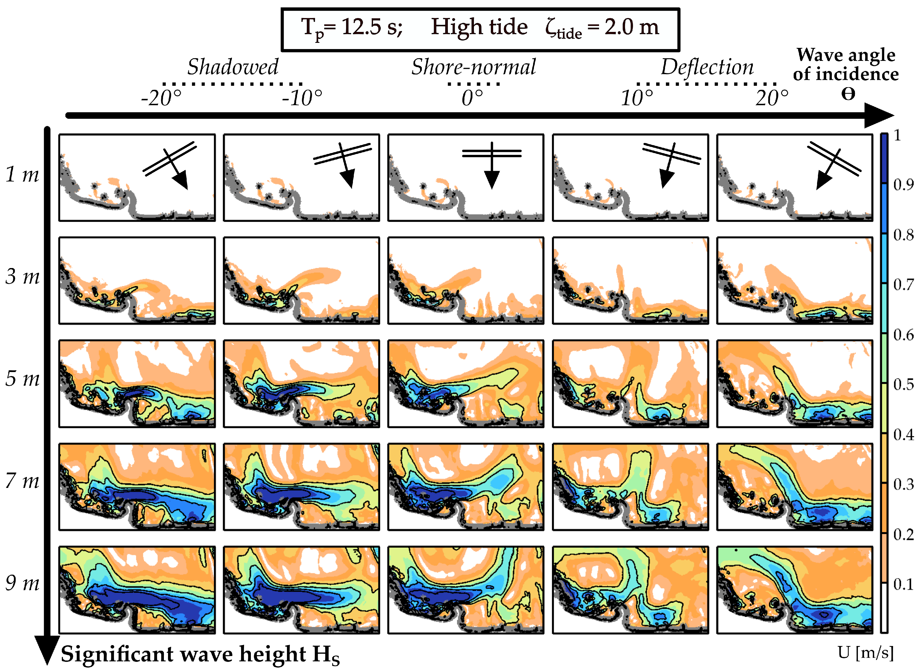
The deflection mechanism along PCA-GPB has been identified for one specific wave event. To explore the headland rip pattern response under a broader range of offshore wave conditions, the model is forced by a Jonswap spectrum with varying offshore significant wave height and angle of incidence. The offshore significant wave height is varied from 1 to 9 m while the offshore angle of incidence is varied from to , therefore including the shadowed, shore-normal (relative to PCA) and deflection configuration (Figure 11). The tide level is kept constant and is set to 2.0 m corresponding to a high tide. The other Jonswap parameter values are kept as default: the offshore peak wave period is set to 12.5 s, the peak enhancement factor to 3.3 and the directional wave spreading to . It should be noted that changing the value of does not significantly change modelled mean flow patterns (not shown).
Figure 11 emphasises contrasting circulation patterns depending on offshore wave conditions, in particular the angle of wave incidence. Overall, for shadowed configurations and < 5 m, the longshore current coming from GPB is deflected seaward by the headland creating a deflection rip directed towards PCA. The seaward portion of deflected longshore current decreases as the offshore wave height increases ( > 5 m). For very large waves, the longshore current is essentially transmitted to the other side of the headland. This mechanism is similar to the one from Scott et al. [6]. Note that the angle of wave incidence , which is not included within , plays an important role in determining the circulation pattern for natural, asymmetric, headland/embayments. For a given , the longshore current at GPB will be more deflected seaward by the headland as waves become shore-normal relative to PCA. For deflection configurations, the PCA longshore current is fully deflected seaward, regardless of and . The deflection rip head inclination is affected by the offshore wave angle of incidence, with a more skewed rip head as waves become more oblique. These results indicate that the deflection mechanism identified in Section 3.2 is also present for any deflection configuration.
4. Discussion
In this study, a 2DH wave group-resolving model was calibrated and validated against wave and current measurements collected against a 500-m rocky headland during two deflection wave events. During the low-energy wave event, the offshore extent of the rip was underestimated by the model (Figure 6) and may result from the vertical shear of the flow far offshore the breaking point. Such depth dependence has been previously identified for channel rips e.g., [33] and typically consists of a depth-uniform and -varying flow inside and outside the surf zone, respectively. Outside the surf zone, the depth-varying rip flow is commonly characterised by high velocities near the surface and low velocities near the bottom, therefore resulting in underestimated surface flow velocities in the depth-averaged model. The latter constitutes a model limitation that could be potentially improved using three-dimensional (3D) modelling approaches. Such approaches are still computationally expensive for large domains and long event durations making phase-averaged 3D models the most suitable approach to study deflection rips at Anglet-Biarritz.
During the high-energy wave event, VLF fluctuations of the rip were very energetic. Energy levels and characteristic periods of these fluctuations measured 800-m offshore around low tide were well reproduced by the surfbeat model. A sensitivity study of the morphology to nearshore flow patterns has shown that the presence of offshore bedrocks and the sand deposit lobe leads to longshore variations of the longshore current along Anglet beaches which was found to be related to longshore variations of wave heights at the breaking point (not shown). While the mean deflection patterns were not strongly impacted by such variations, the latter can contribute, through longshore variations of radiation stress gradients, to very-flow-frequency motions [34]. The present paper serves as a model validation step for reproducing VLF motions and the driving mechanism of these motions is currently under investigation.
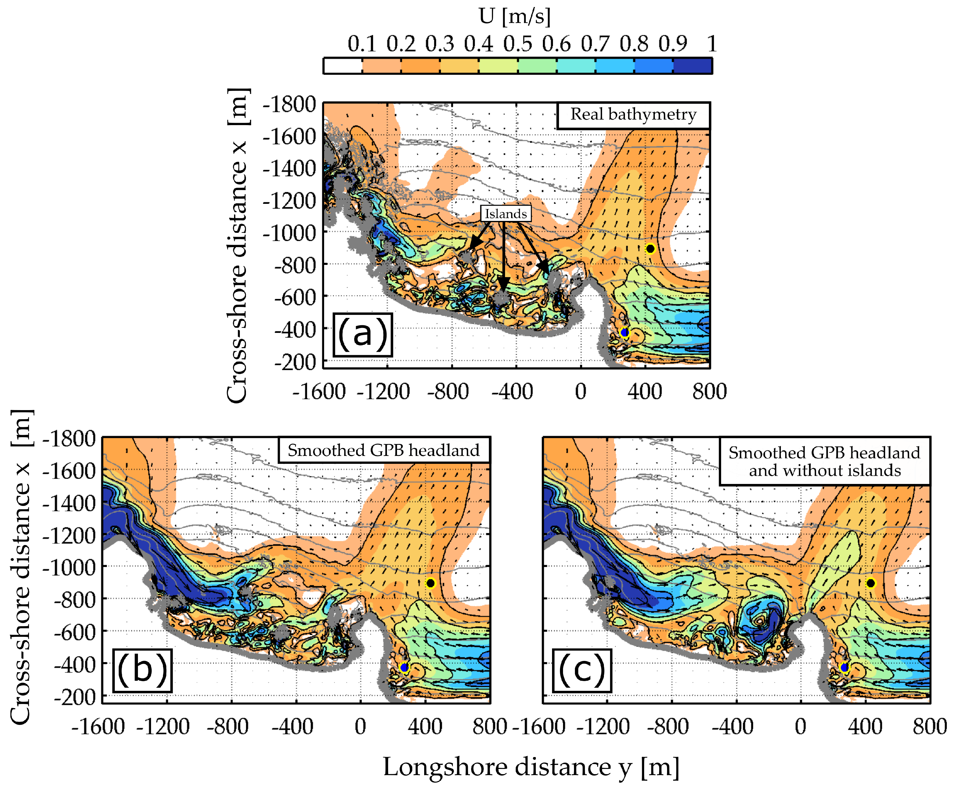
The synoptic flow behaviour during the high-energy wave event indicates that the deflection rip extended approximately 1400 m seawards, corresponding to two to three surf zone widths, at both low tide and high tide (Figure 9). At low tide, the surf zone edge extended seaward of the headland tip and the longshore current was fully deflected offshore by the headland and the current coming from the adjacent embayment. The intensity of adjacent embayment current may be potentially overestimated by the model as the modelled and measured deflection rip head orientations were slightly different. Further instrument deployments are required to better characterise the rip flow along the adjacent embayment. The synoptic flow behaviour essentially highlights a deflection mechanism different from traditional deflection patterns conceptualized around groynes. Simulations on idealised bathymetries pointed out the crucial role of adjacent embayments in the deflection pattern under high-energy wave conditions. Further simulations with smoothed bathymetry were performed to assess the morphological control on the circulation along the adjacent embayment (see Appendix B). They suggest that the morphological setup of the GPB (e.g., curved shape, orientation) is responsible for the longshore current along the adjacent embayment. More broadly, this paper shows that circulation patterns against headlands and along embayments are strongly controlled by the natural variability of the morphology. The results of this study have implications for headland bypassing which is a critical component of the embayment sediment budget. Based on the findings of [6,35] attempted to parametrise headland bypassing along an isolated headland as a function of the boundary length to surf zone width ratio. Their empirical formula was further tested against 29 natural headlands and extended to include morphological parameters such as the headland toe depth [19]. Here, the adjacent embayment is shown to be a critical morphological parameter for the quantification of headland bypassing. For high-energy wave events examined in this paper, multi-embayment circulation occurs, under which adjacent embayment circulation interacts with the rip against the headland of interest. This type of circulation was first described by McCarroll et al. [36] and further identified by Valiente et al. [37]. Under these conditions, bypass formulas should be applied with caution [35]. Further modelling is required to include the effect of adjacent embayment into headland bypassing expression.
5. Conclusions
An XBeach surfbeat model was implemented to explore the dynamics of natural headland rips under a broad range of incident wave conditions and tide level. The model was calibrated and extensively validated against data collected in the vicinity of a 500-m rocky headland during two deflection wave events. Overall, the bulk hydrodynamics parameters were well computed by the model for both events. In particular, the model was able to reproduce time-averaged velocities and the strong tidal modulation of deflection rips. During the high-energy wave event, the amplitude and period of fluctuations of the rip at the VLF time scale were successfully simulated by the 2DH wave group-resolving model. These findings indicate that a 2DH model is able to reproduce the spatio-temporal variability of natural headland rips. The use of 3D phase-averaged models to potentially improve the results of this study will be tested in the future.
The validated model was further used to draw a synoptic flow behaviour of the large-scale deflection rips and examine the spatio-temporal variability of natural headland rips under different wave conditions. Unlike traditional deflection rip patterns, the longshore current was found to be fully deflected offshore, regardless of the boundary length to surf zone width ratio, creating a deflection rip extending two to three surf zone widths offshore. Under deflection configurations, the deflection pattern identified during one specific high-energy event was similar when varying the offshore wave height and angle of incidence. Simulations on idealised bathymetries allowed to assess the morphological control on the deflection rip patterns and showed the adjacent embayment to be responsible for the seaward extent of the headland rip under energetic wave conditions. More broadly, this study shows that the circulation patterns along natural rugged coastlines are strongly controlled by the natural variability of the coastal morphology, including headland shape and adjacent embayment(s). In this context, headland bypassing expression should be applied with caution and further refined to take into account these characteristics.
Author Contributions
Conceptualization, A.M., P.B., B.C. and K.M.; methodology, A.M., P.B., B.C. and K.M.; software, A.M. and K.M.; validation, A.M., P.B., B.C. and K.M.; formal analysis, A.M., P.B., B.C. and K.M.; investigation, A.M., P.B., B.C. and K.M.; resources, P.B. and B.C.; data curation, A.M.; writing—original draft preparation, A.M.; writing—review and editing, A.M., P.B., B.C. and K.M.; visualization, A.M.; project administration, P.B.; funding acquisition, P.B. All authors have read and agreed to the published version of the manuscript.
Funding
This research was funded by the projet MEPELS (contract number 18CP05), performed under the auspices of the DGA and led by SHOM.
Institutional Review Board Statement
Not applicable.
Informed Consent Statement
Not applicable.
Conflicts of Interest
The authors declare no conflict of interest.
Appendix A. Model Description
Based on the input offshore directional wave spectrum, times series of the free surface elevation are generated using random phase summation along the offshore wave boundary. They are Hilbert-transformed to obtain time series of the incoming short-wave energy varying at the wave group scale. Such energy is then propagated and dissipated through the model domain using the following wave-action balance:
where x and y are the cross-shore and longshore coordinates, respectively. , and are the wave action, the wave energy density and the radial frequency, respectively. The mean wave direction and the group velocity are both computed using a stationary wave model [32]. This method allows to preserve wave groupiness over large distances, which in turn allows to properly compute nearshore infragravity motions.
The dissipation of wave energy due to breaking is computed following [38] as function of the so-called breaking parameter . To take into account the roller effect on the circulation, acts as a source term in the roller energy balance which is fully described in [25,39].
Spatial gradients of radiation stress including both wave and roller contributions force currents and surface elevation varying at the wave-group (infragravity) scale with the following non-linear shallow water equations:
In Equation (A2), and are the cross-shore and longshore components of radiation stress gradients, respectively. is the surface elevation, and are the cross-shore and longshore Lagrangian velocities, respectively. Along the offshore boundary, Equation (A2) are forced with the incoming bound wave computed following [31].
The bottom friction associated with currents and infragravity waves is parametrised with
where , and are the Eulerian velocities and the orbital velocity, respectively. is a dimensionless bottom friction coefficient:
with C the Chezy value constant over space and time.
The lateral momentum mixing is parametrized using an eddy viscosity . The latter can be set as a constant value over space and time or can be varied over space and time using the Smagoringsky model. In the present study, the eddy viscosity was set to its default value which a constant value of 0.5 m/s.
Appendix B. Morphological Control on the Circulation along the Adjacent Embayment
Figure A1.
Modelled velocity fields along the adjacent embayment for three idealised bathymetries: real bathymetry (a), smoother GBP headland (b) and removing the GPB islands (c).
Figure A1.
Modelled velocity fields along the adjacent embayment for three idealised bathymetries: real bathymetry (a), smoother GBP headland (b) and removing the GPB islands (c).

References
- Shepard, F.P.; Emery, K.O.; La Fond, E.C. Rip Currents: A Process of Geological Importance. J. Geol. 1941, 49, 337–369. [Google Scholar] [CrossRef]
- Bowen, A.J. Rip currents: 1. Theoretical investigations. J. Geophys. Res. 1969, 74, 5467–5478. [Google Scholar] [CrossRef]
- Castelle, B.; Scott, T.; Brander, R.; McCarroll, R. Rip current types, circulation and hazard. Earth-Sci. Rev. 2016, 163, 1–21. [Google Scholar] [CrossRef]
- Bruneau, N.; Castelle, B.; Bonneton, P.; Pedreros, R.; Almar, R.; Bonneton, N.; Bretel, P.; Parisot, J.P.; Sénéchal, N. Field observations of an evolving rip current on a meso-macrotidal well-developed inner bar and rip morphology. Cont. Shelf Res. 2009, 29, 1650–1662. [Google Scholar] [CrossRef]
- Pattiaratchi, C.; Olsson, D.; Hetzel, Y.; Lowe, R. Wave-driven circulation patterns in the lee of groynes. Cont. Shelf Res. 2009, 29, 1961–1974. [Google Scholar] [CrossRef]
- Scott, T.; Austin, M.; Masselink, G.; Russell, P. Dynamics of rip currents associated with groynes — field measurements, modelling and implications for beach safety. Coast. Eng. 2016, 107, 53–69. [Google Scholar] [CrossRef] [Green Version]
- MacMahan, J.H.; Thornton, E.B.; Stanton, T.P.; Reniers, A.J. RIPEX: Observations of a rip current system. Mar. Geol. 2005, 218, 113–134. [Google Scholar] [CrossRef] [Green Version]
- Austin, M.; Scott, T.; Brown, J.; Brown, J.; MacMahan, J.; Masselink, G.; Russell, P. Temporal observations of rip current circulation on a macro-tidal beach. Cont. Shelf Res. 2010, 30, 1149–1165. [Google Scholar] [CrossRef]
- Castelle, B.; Michallet, H.; Marieu, V.; Leckler, F.; Dubardier, B.; Lambert, A.; Berni, C.; Bonneton, P.; Barthélemy, E.; Bouchette, F. Laboratory experiment on rip current circulations over a moveable bed: Drifter measurements. J. Geophys. Res. 2010, 115, C12008. [Google Scholar] [CrossRef] [Green Version]
- Castelle, B.; Coco, G. Surf zone flushing on embayed beaches: EMBAYED BEACH FLUSHING. Geophys. Res. Lett. 2013, 40, 2206–2210. [Google Scholar] [CrossRef] [Green Version]
- Short, A.D. Role of geological inheritance in Australian beach morphodynamics. Coast. Eng. 2010, 57, 92–97. [Google Scholar] [CrossRef]
- Scott, T.; Masselink, G.; Russell, P. Morphodynamic characteristics and classification of beaches in England and Wales. Mar. Geol. 2011, 286, 1–20. [Google Scholar] [CrossRef] [Green Version]
- Short, A.D.; Masselink, G. Embayed and structurally controlled beaches. In Handbook of Beach and Shoreface Morphodynamics; Wiley: New York, NY, USA, 1999; pp. 230–250. [Google Scholar]
- Castelle, B.; Coco, G. The morphodynamics of rip channels on embayed beaches. Cont. Shelf Res. 2012, 43, 10–23. [Google Scholar] [CrossRef]
- Coutts-Smith, A.J. The Significance of Mega-Rips Along an Embayed Coast. Ph.D. Thesis, University of Sydney, Sydney, Australia, 2004. [Google Scholar]
- McCarroll, R.J.; Brander, R.W.; Turner, I.L.; Power, H.E.; Mortlock, T.R. Lagrangian observations of circulation on an embayed beach with headland rip currents. Mar. Geol. 2014, 355, 173–188. [Google Scholar] [CrossRef]
- McCarroll, R.J.; Brander, R.W.; Scott, T.; Castelle, B. Bathymetric Controls on Rotational Surfzone Currents. J. Geophys. Res. Earth Surf. 2018, 123, 1295–1316. [Google Scholar] [CrossRef]
- Valiente, N.G.; McCarroll, R.J.; Masselink, G.; Scott, T.; Wiggins, M. Multi-annual embayment sediment dynamics involving headland bypassing and sediment exchange across the depth of closure. Geomorphology 2019, 343, 48–64. [Google Scholar] [CrossRef]
- King, E.V.; Conley, D.C.; Masselink, G.; Leonardi, N.; McCarroll, R.J.; Scott, T.; Valiente, N.G. Wave, Tide and Topographical Controls on Headland Sand Bypassing. J. Geophys. Res. Ocean. 2021, 126. [Google Scholar] [CrossRef]
- Loureiro, C.; Ferreira, Ó.; Cooper, J.A.G. Extreme erosion on high-energy embayed beaches: Influence of megarips and storm grouping. Geomorphology 2012, 139–140, 155–171. [Google Scholar] [CrossRef]
- Vieira da Silva, G.; Toldo, E.E.; Klein, A.H.d.F.; Short, A.D.; Woodroffe, C.D. Headland sand bypassing—Quantification of net sediment transport in embayed beaches, Santa Catarina Island North Shore, Southern Brazil. Mar. Geol. 2016, 379, 13–27. [Google Scholar] [CrossRef]
- Mouragues, A.; Bonneton, P.; Castelle, B.; Marieu, V.; Barrett, A.; Bonneton, N.; Detand, G.; Martins, K.; McCarroll, J.; Morichon, D.; et al. Field Observations of Wave-induced Headland Rips. J. Coast. Res. 2020, 95, 578. [Google Scholar] [CrossRef]
- Mouragues, A.; Bonneton, P.; Castelle, B.; Marieu, V.; McCarroll, R.J.; Rodriguez-Padilla, I.; Scott, T.; Sous, D. High-energy surf zone currents and headland rips at a geologically-constrained mesotidal beach. J. Geophys. Res. Ocean. 2020. [Google Scholar] [CrossRef]
- Abadie, S.; Butel, R.; Dupuis, H.; Brière, C. Paramètres statistiques de la houle au large de la côte sud-aquitaine. Comptes Rendus Geosci. 2005, 337, 769–776. [Google Scholar] [CrossRef]
- Roelvink, D.; Reniers, A.; van Dongeren, A.; van Thiel de Vries, J.; McCall, R.; Lescinski, J. Modelling storm impacts on beaches, dunes and barrier islands. Coast. Eng. 2009, 56, 1133–1152. [Google Scholar] [CrossRef]
- Austin, M.J.; Scott, T.; Russell, P.; Masselink, G. Rip Current Prediction: Development, Validation, and Evaluation of an Operational Tool. J. Coast. Res. 2012, 29, 283. [Google Scholar] [CrossRef] [Green Version]
- Reniers, A.; MacMahan, J.; Thornton, E.; Stanton, T. Modelling infragravity motions on a rip-channel beach. Coast. Eng. 2006, 53, 209–222. [Google Scholar] [CrossRef] [Green Version]
- Reniers, A.J.H.M.; MacMahan, J.H.; Thornton, E.B.; Stanton, T.P. Modeling of very low frequency motions during RIPEX. J. Geophys. Res. 2007, 112, C07013. [Google Scholar] [CrossRef] [Green Version]
- Bellafont, F.; Morichon, D.; Roeber, V.; André, G.; Abadie, S. Infragravity period oscillations in a channel harbor near a river mouth. Coast. Eng. Proc. 2018, 1. [Google Scholar] [CrossRef]
- Varing, A.; Filipot, J.F.; Delpey, M.; Guitton, G.; Collard, F.; Platzer, P.; Roeber, V.; Morichon, D. Spatial distribution of wave energy over complex coastal bathymetries: Development of methodologies for comparing modeled wave fields with satellite observations. Coast. Eng. 2020, 169. [Google Scholar] [CrossRef]
- Herbers, T.H.C.; Elgar, S.; Guza, R.T. Infragravity-Frequency (0.005–0.05 Hz) Motions on the Shelf. Part I: Forced Waves. J. Phys. Oceanogr. 1994, 24, 917–927. [Google Scholar] [CrossRef]
- Roelvink, D.; McCall, R.; Mehvar, S.; Nederhoff, K.; Dastgheib, A. Improving predictions of swash dynamics in XBeach: The role of groupiness and incident-band runup. Coast. Eng. 2018, 134, 103–123. [Google Scholar] [CrossRef]
- Haas, K.A.; Svendsen, I.A. Laboratory measurements of the vertical structure of rip currents. J. Geophys. Res. Ocean. 2002, 107, 15-1–15-9. [Google Scholar] [CrossRef]
- Newberger, P.A.; Allen, J.S. Forcing a three-dimensional, hydrostatic, primitive-equation model for application in the surf zone: 2. Application to DUCK94. J. Geophys. Res. 2007, 112, C08019. [Google Scholar] [CrossRef] [Green Version]
- McCarroll, R.J.; Masselink, G.; Valiente, N.G.; King, E.V.; Scott, T.; Stokes, C.; Wiggins, M. An XBeach derived parametric expression for headland bypassing. Coast. Eng. 2021, 165, 103860. [Google Scholar] [CrossRef]
- McCarroll, R.; Masselink, G.; Valiente, N.; Scott, T.; King, E.; Conley, D. Wave and Tidal Controls on Embayment Circulation and Headland Bypassing for an Exposed, Macrotidal Site. J. Mar. Sci. Eng. 2018, 6, 94. [Google Scholar] [CrossRef] [Green Version]
- Valiente, N.G.; Masselink, G.; McCarroll, R.J.; Scott, T.; Conley, D.; King, E. Nearshore sediment pathways and potential sediment budgets in embayed settings over a multi-annual timescale. Mar. Geol. 2020, 427, 106270. [Google Scholar] [CrossRef]
- Roelvink, J. Dissipation in random wave groups incident on a beach. Coast. Eng. 1993, 19, 127–150. [Google Scholar] [CrossRef]
- Reniers, A.J.H.M. Morphodynamic modeling of an embayed beach under wave group forcing. J. Geophys. Res. 2004, 109, C01030. [Google Scholar] [CrossRef]
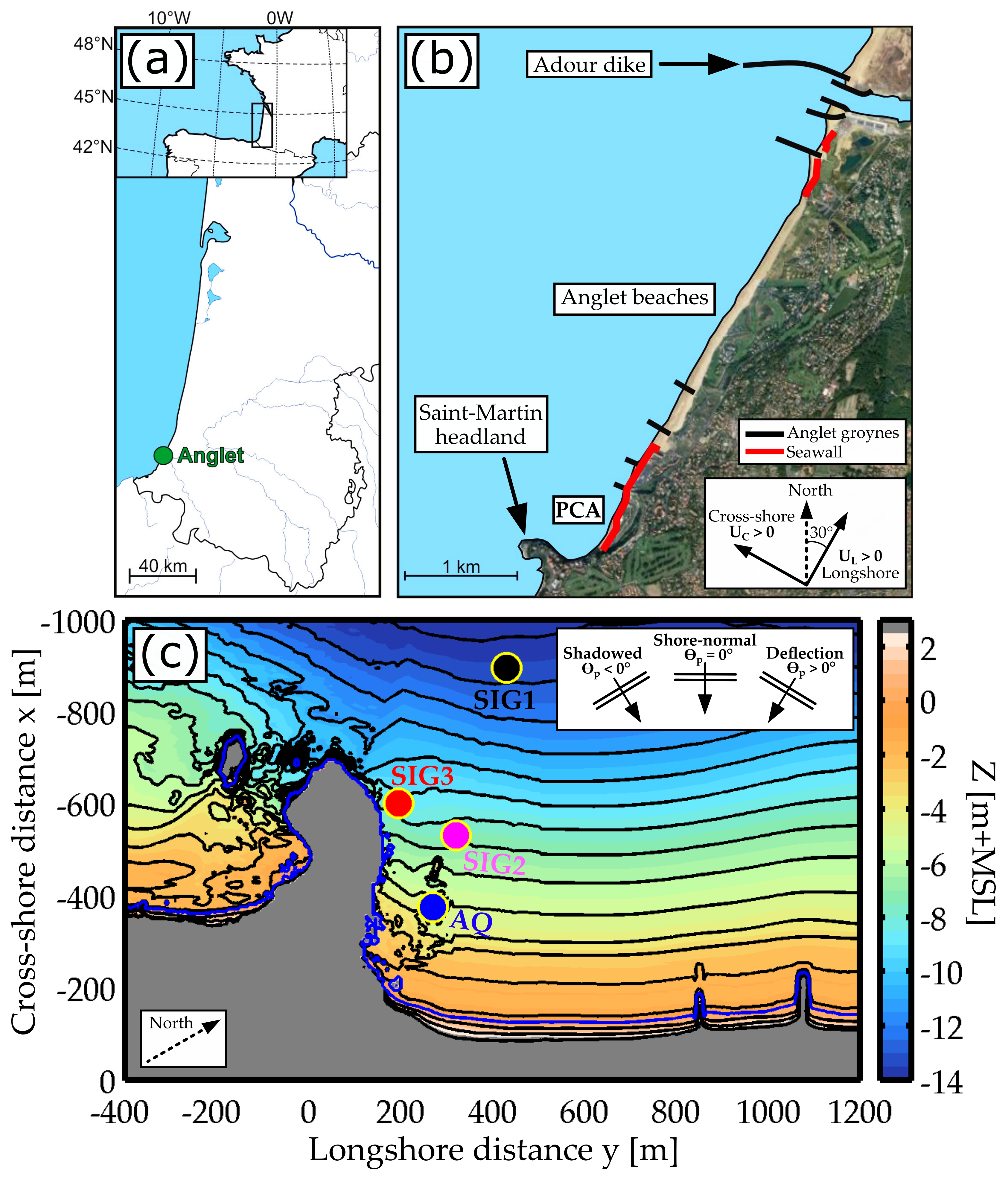
Figure 1.
(a) Location of Anglet along the Aquitaine south coast (SW France). (b) Map of Anglet beaches showing the location of PCA, the Saint Martin headland, the groynes and the Adour dike. and are the cross-shore and longshore velocities, respectively. (c) Bathymetry map of the field site. Colour indicates elevation (Z) relative to mean sea level (MSL), with the blue contour showing the MSL. Black contours are at 1-m separation. Coloured points show measurement locations (SIG1, SIG2, SIG3 and AQ).

Figure 2.
(a) Bathymetry used within the model. Colour indicates elevation (m + MSL), with the blue contour showing the MSL. Black contours are at 2-m separation. (b,c) show the cross-shore () and longshore () mesh step size, respectively.
Figure 2.
(a) Bathymetry used within the model. Colour indicates elevation (m + MSL), with the blue contour showing the MSL. Black contours are at 2-m separation. (b,c) show the cross-shore () and longshore () mesh step size, respectively.

Figure 3.
Offshore wave and tide conditions during the field experiment, with low- and high-energy deflection event (D1 and D2 shown by shaded areas). (a) Tidal level (; blue line; see right axis) and significant wave height (; black line). (b) Peak wave period (; blue dots) and mean wave period (; black line). (c) Peak wave angle of incidence with respect to the shore normal (; blue dots) and its 12h-averaged values (black line). Positive values mean a deflection configuration (see Figure 1c).

Figure 4.
Measurements (subscript M) versus model (subscript XB) for events D1 and D2 and for each instrument. (a) Significant short wave height ( and ); (b) Significant infragravity wave height ( and ); (c) 30 min-averaged velocity magnitude ( and ). The corresponding coefficient of correlation and normalized root-mean-squared error (NRMSE) are indicated in each panel.

Figure 5.
Modelled mean water depth (; top panels). Modelled (black) and measured (blue) 5 min running-averaged cross-shore (; middle panels) and longshore velocities (; bottom panels) for event D1 at SIG2 and SIG3 locations. Note that AQ was not measuring at this time. Black line and grey area show the modelled velocities of one simulation and the confidence interval computed from ten simulations (see Section 2.3).

Figure 6.
Mean Lagrangian velocity field measured at the surface (Drifter measurements; left panel) and mean modelled velocity field (XB-SB; right panel) interpolated onto the drifter grid. The top white square shows the period of averaging and the corresponding offshore wave conditions (, , ) and tide level ().

Figure 7.
Modelled mean water depth (; top panels). Modelled (black) and measured (blue) 5 min running-averaged cross-shore (; middle panels) and longshore velocities (; bottom panels) for event D2 at SIG1 and AQ locations. Note that measurements at SIG2 and SIG3 were not available at this time. Black line and grey area show the modelled velocities of one simulation and the confidence interval computed from ten simulations (see Section 2.3).

Figure 8.
Modelled (black; one simulation) and measured (blue) velocity magnitude spectrum at low tide of event D2. Black vertical lines indicate the very low frequency band (VLF; f < 0.004 Hz) and the infragravity band (IG; 0.004 Hz < f < 0.04 Hz) at SIG1 and AQ (top and bottom panels, respectively). For each panel, the root mean square VLF velocity magnitudes computed following Reniers et al. [28] are indicated. is the data while and are the mean rms magnitude averaged over ten simulations and its corresponding standard deviation, respectively.

Figure 9.
Modelled velocity field averaged at low tide (left) and high tide (right) of the high-energy deflection event. For each panel, the top-right white square shows the period of averaging, the corresponding offshore wave conditions (, , ) and tide level (). The red line represents the outer edge of the surf zone computed as the cross-shore location where wave dissipation reaches 10% of its cross-shore maximum (similar to [6]).

Figure 10.
Model output at low tide of event D2 for three bathymetries: real bathymetry, excluding offshore bathymetry features and excluding the adjacent embayment. Top panels: modelled 5 min-running averaged velocity magnitudes during the first low tide of event D2 at SIG1 (a) and AQ (b) locations. Bottom panels (c–e): modelled mean velocity field plotted on the magnitude contours (0.2-m/s spaced; black lines) and the bathymetry contours (2-m spaced; grey lines), averaged at low tide of event D2. The black and blue points indicate SIG1 and AQ locations, respectively.

Figure 11.
Modelled mean velocity field under various offshore significant wave height and wave angle of incidence at high tide ( = 2.0 m). Black lines indicate the 0.4, 0.6, 0.8 and 1.0 m/s contours. The grey line shows the mean sea level contour.
Figure 11.
Modelled mean velocity field under various offshore significant wave height and wave angle of incidence at high tide ( = 2.0 m). Black lines indicate the 0.4, 0.6, 0.8 and 1.0 m/s contours. The grey line shows the mean sea level contour.


Table 1.
Root-mean-squared error (RMSE) and its normalized value (NRMSE) computed for each event and at each instrument location.
Table 1.
Root-mean-squared error (RMSE) and its normalized value (NRMSE) computed for each event and at each instrument location.
| Events | Statistics | Bulk Quantities | SIG1 | SIG2 | SIG3 | AQ |
|---|---|---|---|---|---|---|
| D1 | RMSE | 0.19 m | 0.20 m | 0.29 m | - | |
| 0.02 m | 0.05 m | 0.04 m | - | |||
| 0.03 | 0.09 | 0.06 | - | |||
| NRMSE (%) | 12.5 | 12.8 | 19.9 | - | ||
| 15.0 | 27.4 | 21.0 | - | |||
| 28.9 | 22.1 | 20.2 | - | |||
| D2 | RMSE | 0.29 m | - | - | 10.1 m | |
| 0.08 m | - | - | 15.7 m | |||
| 0.15 | - | - | 0.20 | |||
| NRMSE (%) | 9.4 | - | - | 11.1 | ||
| 24.3 | - | - | 19.6 | |||
| 30.5 | - | - | 28.4 |
Publisher’s Note: MDPI stays neutral with regard to jurisdictional claims in published maps and institutional affiliations. |
© 2021 by the authors. Licensee MDPI, Basel, Switzerland. This article is an open access article distributed under the terms and conditions of the Creative Commons Attribution (CC BY) license (https://creativecommons.org/licenses/by/4.0/).
Share and Cite
MDPI and ACS Style
Mouragues, A.; Bonneton, P.; Castelle, B.; Martins, K. Headland Rip Modelling at a Natural Beach under High-Energy Wave Conditions. J. Mar. Sci. Eng. 2021, 9, 1161. https://doi.org/10.3390/jmse9111161
AMA Style
Mouragues A, Bonneton P, Castelle B, Martins K. Headland Rip Modelling at a Natural Beach under High-Energy Wave Conditions. Journal of Marine Science and Engineering. 2021; 9(11):1161. https://doi.org/10.3390/jmse9111161
Chicago/Turabian StyleMouragues, Arthur, Philippe Bonneton, Bruno Castelle, and Kévin Martins. 2021. "Headland Rip Modelling at a Natural Beach under High-Energy Wave Conditions" Journal of Marine Science and Engineering 9, no. 11: 1161. https://doi.org/10.3390/jmse9111161
Note that from the first issue of 2016, this journal uses article numbers instead of page numbers. See further details here.