Monitoring and Forecasting the Ocean State and Biogeochemical Processes in the Black Sea: Recent Developments in the Copernicus Marine Service

Abstract

The Black Sea Monitoring and Forecasting Center (BS-MFC) is the European reference service for the provision of ocean analyses, forecasts, and reanalyses in the Black Sea basin. It is part of the Copernicus Marine Environment and Monitoring Service (CMEMS) and ensures a high level of efficiency in terms of operations, science, and technology for predictions and the monitoring of physical and biogeochemical processes in the Black Sea. The operational BS-MFC framework is based on state-of-the-art numerical models for hydrodynamics, biogeochemistry, and waves; analysis, forecast, and reanalysis are provided on a spatial grid with about 3 km of horizontal resolution that covers the whole Black Sea basin (the Azov Sea is not included). The scientific assessment of BS-MFC products is performed by implementing a product quality dashboard that provides pre-qualification and operational model skills according to GODAE/OceanPredict standards. Novel interfaces based on high-resolution models are part of the scientific development plan to ensure a strong connection with the nearest seas from a modelling point of view, in particular with the Mediterranean Sea. To improve forecasting skills, dedicated online coupled systems are being developed, which involve physics, biogeochemistry, and waves together with the atmosphere and, in the future, with ensemble forecasting methodologies and river-ocean interfaces.

1. Introduction

Understanding, predicting, and reconstructing the ocean state is globally one of the most challenging objectives for operational oceanography, especially to support user needs as well as down-stream services and applications for what is termed the Blue Growth and the Blue Economy for a Blue Society. In the European panorama, the Black Sea, together with the Azov Sea, the Marmara Sea, and the Mediterranean Sea, is part of a peculiar complex system of marginal seas that is functional to ocean monitoring and climate. Due to particular physical and biogeochemical processes, the Black Sea deserves a more dedicated focus so as to be able to set up a reliable modelling system and observing network for the next generation of operational ocean forecasting systems.

This baseline is one of the main priorities pursued within the Copernicus Marine Environment and Monitoring Service (CMEMS, [1]). The Black Sea Monitoring and Forecasting Center (BS-MFC) is the CMEMS operational service dedicated to the regional needs of the Black Sea, which has been operational since the end of 2016 and serves about 60 “active users” (i.e., users that regularly download CMEMS data) from academia (~30%), public sectors and organizations (~20%), and the business and private sectors (~50%). The main objective of the BS-MFC is to serve the specific needs of the Black Sea countries in decision-making by developing new operational services that are able to protect the marine ecosystem, contrasting pollution and environmental emergencies, supporting maritime safety and routing, and promoting a science-driven cooperation for user-driven applications from the regional to the coastal scale. Access to high-quality operational data related to forecasting and reconstruction of past ocean states in the Black Sea is a pre-requisite for achieving these targets. The BS-MFC is a joint venture between the Institute of Oceanology-Bulgarian Academy of Sciences (IO-BAS, Bulgaria) in the role of coordinator, and the following institutes and universities: the Euro-Mediterranean Center on Climate Change Foundation (CMCC, Italy), the University of Liege (ULiege, Belgium), the Helmholtz-Zentrum Hereon (HEREON, Germany), the Sofia University “St. Kliment Ohridski” (USOF, Bulgaria), and the National Institute of Hydrology and Water Management (NIHWM, Romania).

BS-MFC delivers products for analysis, simulation, forecast, and reanalysis through the CMEMS and maintains a level of efficiency and robustness in operations, ensuring new advances in science for the development of specific products. The BS-MFC catalogue offers products for the Blue Ocean (physics and waves) and the Green Ocean (biogeochemistry) at the regional scale. These include: (a) near-real-time (NRT) datasets—analysis and forecast fields at different frequencies for supporting daily services and down-stream applications; and (b) multi-year (MY) datasets—reanalysis and long-term simulations—at different frequencies to provide an estimate of climate variability and trends.

The present paper provides a complete overview of the current BS modelling systems together with a description of the main operational products delivered through CMEMS interfaces. A detailed description of the BS-MFC components (PHY, BIO, and WAV) is also provided, together with a description of the models and data assimilation capabilities used to improve the accuracy of multi-year and forecasting products (Section 2). Product quality and monitoring capacity are described in Section 3 by showing the operational dashboard used to evaluate the accuracy of the BS-MFC products. The last part of this paper summarizes the main scientific challenges and ongoing developments for the next generation of BS-MFC operational systems (Section 4) together with the conclusions (Section 4).

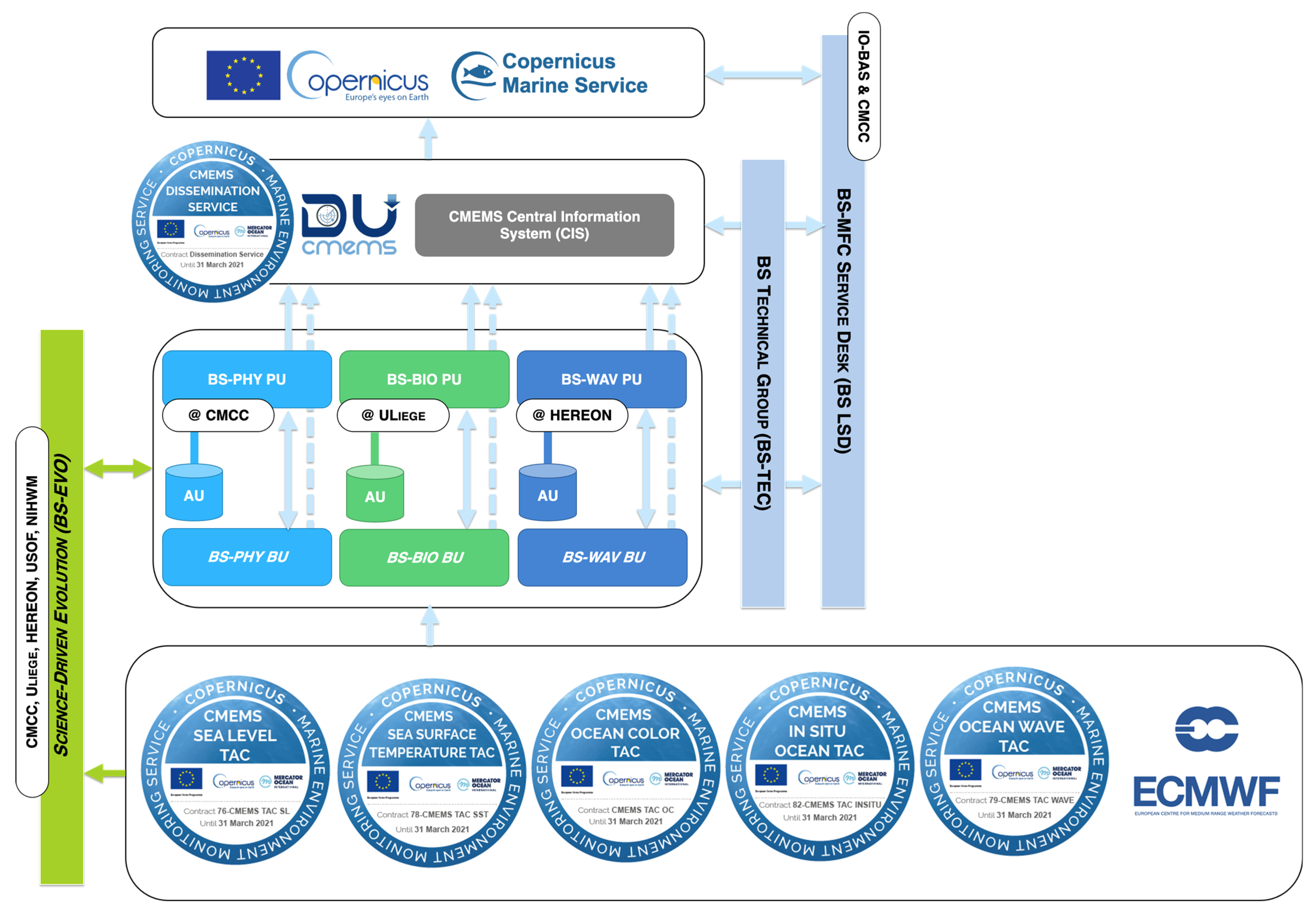
2. The Black Sea MFC High-Level Architecture and Components

The BS-MFC systems provide NRT and MY products over the Black Sea domain (Figure 1), excluding the Azov Sea and the Bosporus Strait, at a resolution of 1/27° in the zonal direction and 1/36° in the meridional direction.

The BS-MFC uses an operational framework based on a high-level architecture, represented in Figure 2. Three production units (PU) are responsible for the system and operational services, including evolutions of the physics (BS-PHY PU), biogeochemistry (BS-BIO PU), and wave (BS-WAV PU) components (run by CMCC, ULiege, and HEREON, respectively). Each PU is connected to its own archiving unit (AU) for the long-term storage of the BS-MFC products, and to a backup unit (BU) in the case of nominal operational failures and recoveries in order to guarantee the continuity of operational services. Additionally, each PU implements dedicated interfaces: (a) with the BS-MFC technical group, for the technical implementation of the product catalogue (BS TEC), (b) with the dissemination unit (DU) through the delivery buffer zone, for the operational delivery of the products (CMEMS CIS), and (c) with the BS-MFC service desk (BS LSD), for user support through the CMEMS service desk. Service evolution activities, aimed at R&D activities, are implemented at the PU level, with the collaboration of USOF and NIHWM (BS-EVO). Observations used by BS-MFC systems for assimilation and validation purposes are summarized in

Table 1. Upstream data dependency for the BS-MFC: for each type of observation, provider and product ID are given as well as the BS component—PHY, BIO, WAV—and product category—NRT and MY—which up-take it for assimilation (A) and/or validation (V).

Type of Observation	Provider	Product ID (If Available)	BS-PHY	BS-BIO	BS-WAV
Temperature and salinity profiles (in situ)	CMEMS	INSITU_BS_NRT_OBSERVATIONS_013_034	A, V (NRT)	V (NRT)	V (NRT)
		INSITU_GLO_TS_REP_OBSERVATIONS_013_001_B	A, V (MY)	V (MY)	A, V (MY)
	SeaDataNet	NA, see [2]	A (MY)
Sea surface temperature (satellite)	CMEMS	SST_BS_SST_L4_NRT_OBSERVATIONS_010_006	A (NRT)
		SST_BS_SST_L3S_NRT_OBSERVATIONS_010_013	V (NRT)
		SST_BS_SST_L4_REP_OBSERVATIONS_010_022	A, V (MY)
Sea level anomaly (satellite)	CMEMS	SEALEV-EL_EUR_PHY_L3_NRT_ OBSERVATIONS_008_059	A, V (MY)
		SEALEV-EL_BS_PHY_L4_REP_OBSERVATIONS_008_042	A, V (MY)
Chlorophyll (satellite)	CMEMS	OCEANCOL-OUR_BS_CHL_L3_NRT_OBSERVATIONS_009_045		A (NRT)
		OCEANCOL-OUR_BS_OPTICS_L3_NRT_OBSERVATIONS_009_04		V (NRT)
		OCEANCOL-OUR_BS_CHL_L3_REP_OBSERVATIONS_009_079		V (MY)
Significant wave height (satellite)	CMEMS	WAVE_GLO_WAV_L3_SWH_NRT_OBSERVATIONS_014_001			V (NRT), A, V (MY)

.

2.1. Physics

The Black Sea physical analysis and forecasting system (BS-PHY NRT) as well as the reanalysis system (BS-PHY MY) are free-surface versions of the NEMO ocean general circulation model (Nucleus for European Modelling of the Ocean, [3]), coupled online with a 3D-variational data assimilation scheme, the OceanVar [4,5]. The model’s governing equations are discretized over a regular grid with about 3 km of horizontal resolution, using 31 z-levels with partial steps over the spatial domain, as shown in Figure 1.

The BS-PHY NRT [6] core model is based on NEMO v3.4. The bottom topography was reconstructed from the GEBCO 1 min resolution dataset [7]. It is forced by water, heat, and momentum fluxes, interactively computed by bulk formulae, implemented for the Mediterranean Forecasting System [8] and modified for the Black Sea to account for the Brunt–Berliand formula for the net longwave radiation, as in [9]. It uses monthly climatological precipitation from the GPCP dataset [10,11] and the 3–6 h and 0.125° operational analysis and forecast atmospheric fields provided by the European Centre for Medium-Range Weather Forecasts (ECMWF) through the Italian Aeronautica Militare.

The model includes 72 rivers, distributed as source points along the Black Sea coastline; major rivers such as the Danube, the Dnieper, and the Dniester are implemented over multi-grid points due to their wide delta and inflow contribution. The river discharge values are provided as monthly climatologies by [12] within the framework of the EU SESAME project, while a zero salinity value is accounted for at the river mouths. Initial conditions for the pre-operational run come from [13] as the climatology for January interpolated on the BS-PHY spatial grid. The model configuration is closed at the Bosporus Strait. Vertical mixing is parameterized according to the turbulent kinetic energy closure scheme.

The assimilation time window is one day. Background error covariances are decomposed into vertical covariances and horizontal correlations through 15-mode multivariate empirical orthogonal functions (EOFs). Observations, assimilated in the BS-PHY NRT, include (Table 1): (i) in situ temperature and salinity profiles (ARGO floats) from the CMEMS INS TAC. If profiles are disseminated at a high vertical resolution, a vertical thinning is applied to the profile before ingestion in OceanVar; (ii) along-track sea level anomaly L3 data, currently from AltiKa, Cryosat-2, and Jason-2/3, Sentinel3A/3B, distributed by the CMEMS SL TAC; (iii) gridded sea surface temperature SST L4 observations provided by the CMEMS SST TAC. Assimilation of SST satellite data is performed at the first model level. For satellite observations (SLA, SST), a horizontal thinning is also applied to retain approximately one observation only every 6 km.

The BS-PHY NRT processing system consists of two different cycles, run every day. One cycle consists of a 3-day analysis (e.g., a simulation performed with ECMWF analysis atmospheric forcing and assimilation correction), a 1-day simulation (e.g., a run performed with ECMWF analysis atmospheric forcing without assimilation correction), and a 10-day forecast (e.g., a run performed with ECMWF forecast atmospheric fields). The other cycle takes place once a week: the system performs a 14-day analysis in order to ingest a larger number of observations through the data assimilation and produce the best initial condition for the forecasting run. The system produces hourly and daily means of 3D temperature, salinity, and currents as well as 2D sea surface height, mixed layer depth, and bottom temperature, with the nominal start of the forecast at 00:00Z (i.e., averaged daily fields are centered at 12:00Z of each run day).

The BS-PHY MY [14] core model is based on NEMO v3.6 over the same spatial grid as the corresponding NRT. The bottom topography has been improved in relation to the NRT system and is based on a GEBCO 30” resolution dataset [15], with the blending of a high-resolution bathymetric dataset around the Bosporus exit [16] to better represent the connection between the Black Sea and the Marmara Sea, and consequently, the Mediterranean Sea. BS-PHY MY system is forced by ECMWF ERA5 atmospheric reanalysis and GPCP monthly climatological precipitation [10,11].

Similarly to the NRT, the BS-PHY MY system imposes a closed boundary condition at the Bosporus Strait. To account for the Mediterranean water inflow into the Black Sea, the model solution is relaxed to temperature and salinity vertical profiles extracted from the high-resolution time series presented in [17]. The model is coupled online with OceanVar to assimilate (i) in situ temperature and salinity profiles (ARGO floats) pro-vided by the CMEMS INS TAC and the historical SeaDataNet dataset [2], (ii) along-track sea level anomaly L3 data distributed by CMEMS SL TAC. The SST is also relaxed to a gridded sea surface temperature SST L4 product produced by the CMEMS SST TAC. The time series covers the period of January 1993–December 2019 and provides monthly and daily means for the 3D temperature, salinity, current and 2D sea-surface height and mixed-layer depth.

2.2. Biogeochemistry

The Black Sea biogeochemical forecasting (BS-BIO NRT, [18]) and reanalysis (BS-BIO MY, [19]) systems are based on the online-coupled Biogeochemical Model for Hypoxic and Benthic Influenced areas (BAMHBI, [20,21,22]) and NEMO v3.6 ([3], version aligned with BS-PHY NRT). The coupled model is run over the same grid as used by BS-PHY NRT, with 31 vertical levels using z-layer vertical coordinates. BAMHBI describes the food web from bacteria to gelatinous carnivores through 24 state variables, including three groups of phytoplankton: diatoms, small phototrophic flagellates, and dinoflagellates; two zooplankton groups: micro- and mesozooplankton; two groups of gelatinous zooplankton: omnivorous and carnivorous forms; and an explicit representation of the bacterial loop: bacteria, labile and semi-labile dissolved organic matter, and particulate organic matter. The model simulates oxygen, nitrogen, silicate, and carbon cycling, and explicitly represents processes in the anoxic layer.

Biogeochemical processes in anaerobic conditions are represented using an approach similar to that used in the modelling of diagenetic processes in sediments, lumping together all the reduced substances in one state variable. Processes in the upper oxygenated layer are thus fully coupled with anaerobic processes in the deep waters, which enable long-term simulations to be performed. This full coupling between aerobic and anaerobic processes is key to performing the long-term reanalysis. Processes typical of anaerobic environments such as denitrification, anaerobic ammonium oxidation (ANAMMOX), and reduced decomposition efficiency are explicitly represented [20,21].

BAMHBI involves a module describing the carbonate dynamics based on the approach proposed by [23]. The model solves for DIC and the Excess Negative charge from which the Total Alkalinity is computed (considering the contribution of sulfide), as well as pH, the speciation of DIC ([HCO₃]⁻, [CO₃]²⁻, [CO₂]), and CO₂ air–sea flux. The model also includes a representation of diagenetic processes [22] using a computationally efficient representation, as proposed by [24].

The incorporation of a benthic module allows for a better representation of the impact of the sedimentary compartment in important biogeochemical processes such as sediment oxygen consumption (which is responsible for the generation of hypoxic conditions in summer), the active degradation of organic matter that determines the vigor of the shelf ecosystem (~30% of the primary production in shelf waters is degraded in the sediment), and the intense consumption of nitrate by benthic denitrification, which filters a substantial part (~50%) of the nitrogen carried by the north-western shelf rivers (the Danube being the most important one) and modulates primary production in the deep basin. In addition to a representation of diagenesis, the biogeochemical model represents the transport of sediments by waves. This is an important feature that is necessary to sustain the primary production of the deep basin.

Every day, the BS-BIO NRT system runs one day of analysis and 10 days of forecasts. Once a week, BS-BIO NRT performs a 10-day analysis during which the model assimilates daily L3 satellite chlorophyll observations (Table 1) via an Ocean Assimilation Kit (OAK) [25], developed as part of the SANGOMA project. The assimilation increments are three-dimensional, i.e., the analysis also modifies the model variables below the surface layer. The BS-BIO NRT system uses ECMWF analysis and forecast atmospheric fields to compute air–sea fluxes, while the BS-BIO MY system uses ECMWF ERA5 reanalysis. Atmospheric fields are used to force NEMO to compute the air–sea exchanges of O₂ and CO₂.

The atmospheric deposition of inorganic nitrogen [26] is also considered. Such a process has a similar order of magnitude as the river inputs and is needed in order to sustain the primary production in the deep basin. For the rivers, due to the absence of operational data, the BS-BIO NRT system uses climatological averages of river flows, inorganic nutrients, and organic material inputs computed from the long-term series of data provided by [12]. In its current configuration, BS-BIO systems (both NRT and MY) involve river inputs from six main rivers: the Danube (split into three branches), Dniepr, Dniestr, Rioni, Sakarya, and Kizilirmak. Water discharges are provided as monthly climatology to capture seasonal signal. The Bosporus Strait is considered an open boundary as in [27] and [28]. The velocity and salinity are determined in such a way that total sea water and salt are conserved in the Black Sea domain.

BS-BIO NRT and MY systems generate the following six datasets:

• NUTR: phosphorus, nitrate;
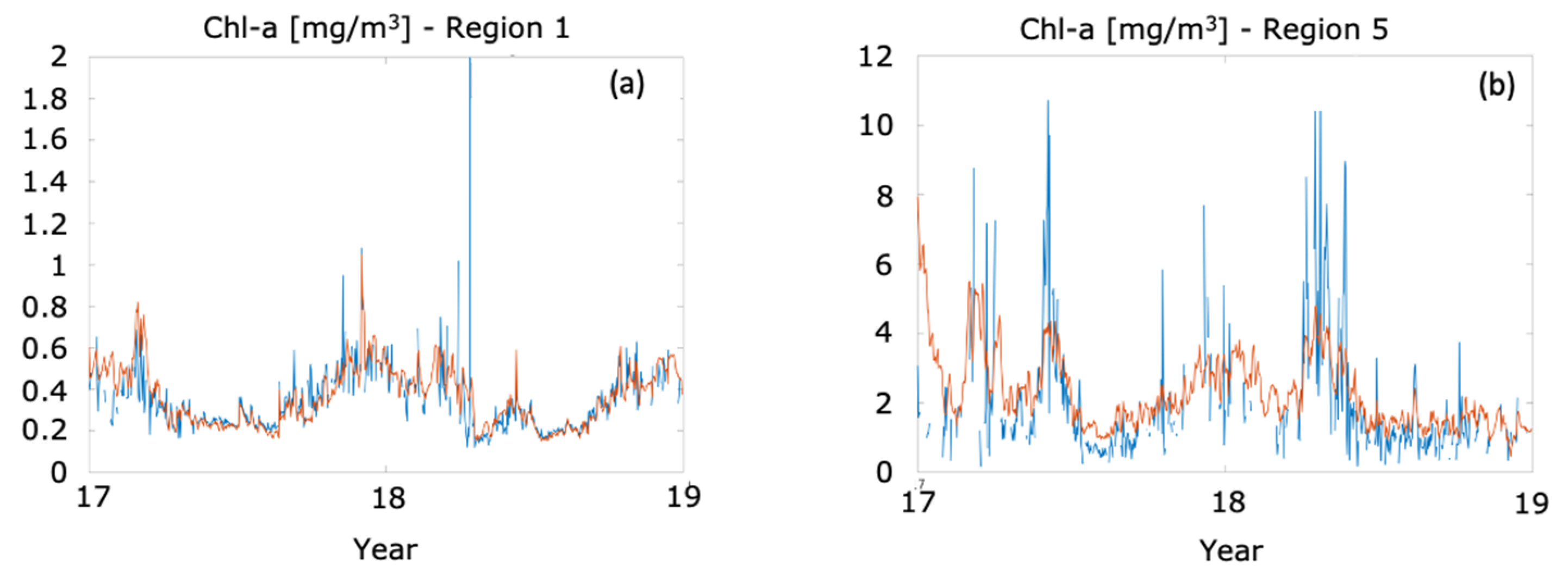
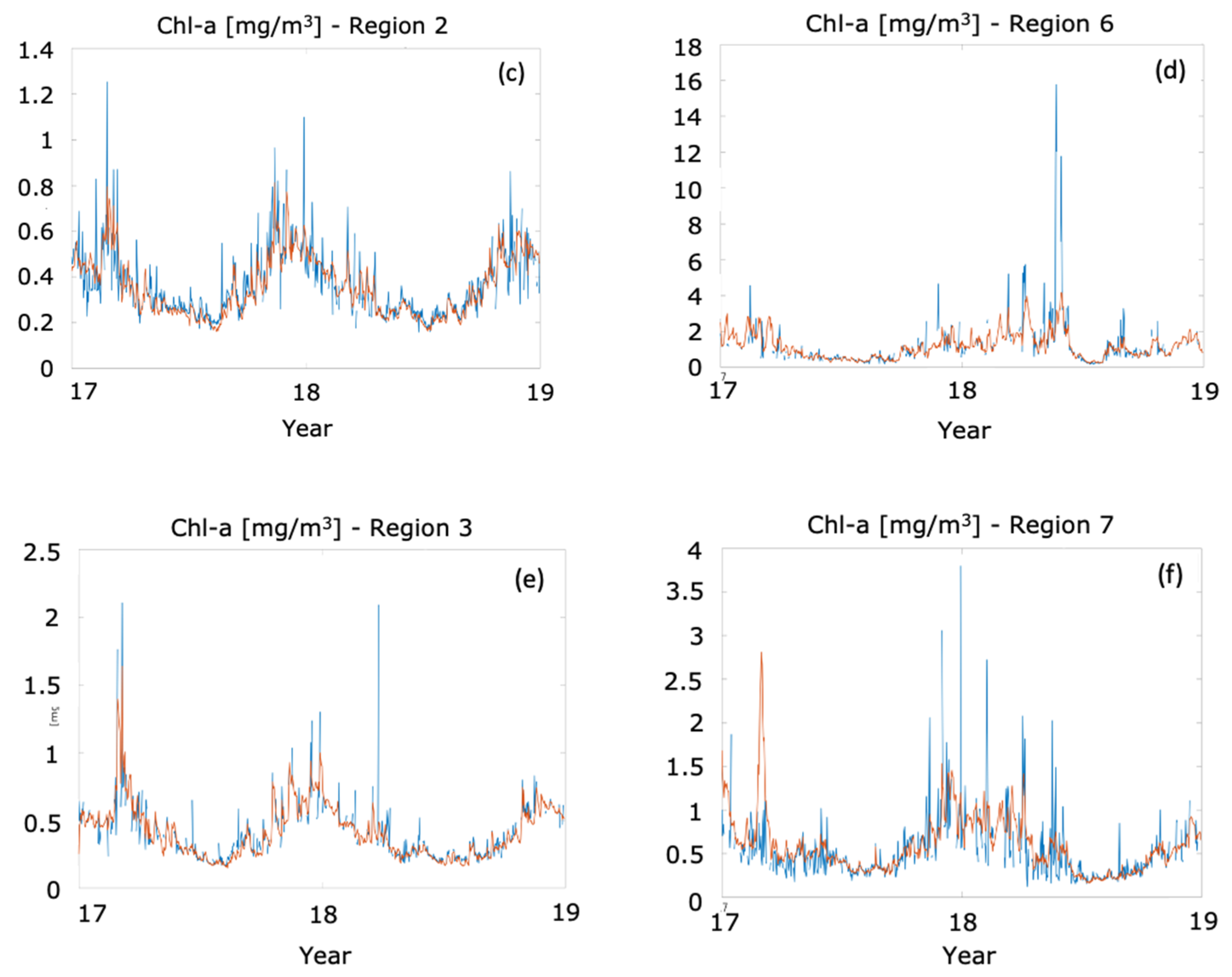
• PFTC: chlorophyll and phytoplankton biomass;
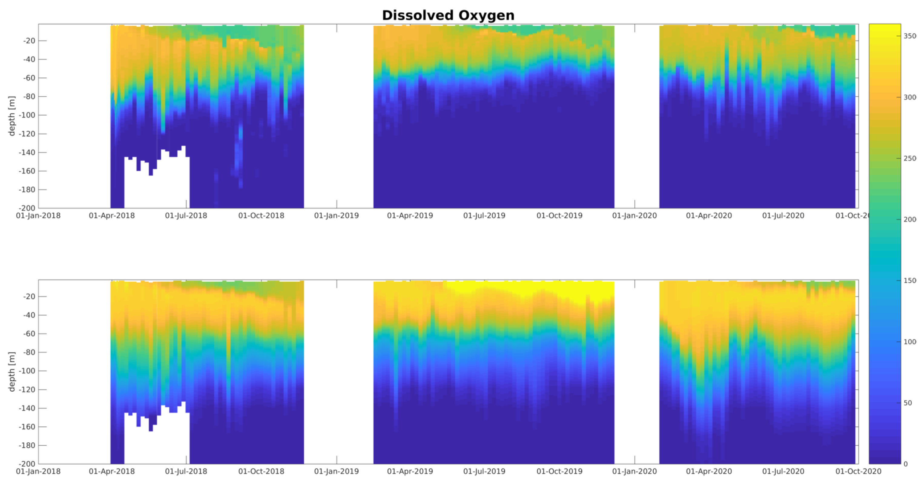
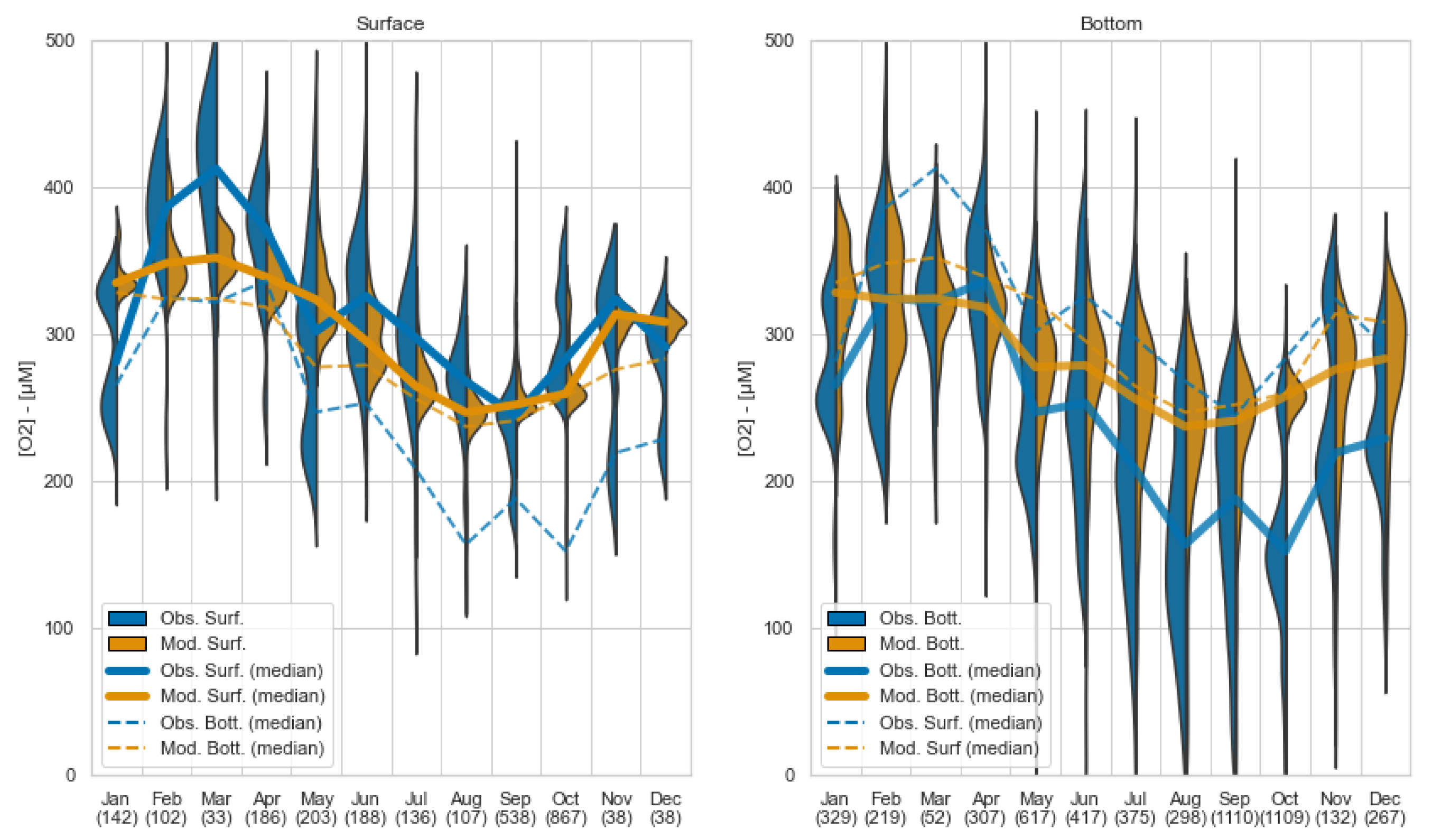
• BIOL: dissolved oxygen (O₂) concentrations and net primary production;
• CARB: pH, dissolved inorganic carbon (DIC), total alkalinity (TA);
• CO₂F: surface partial CO₂ pressure, surface CO₂ flux;
• OPT: photosynthetically active radiation (PAR) and attenuation coefficient (Kd) (only BS-BIO NRT).

2.3. Waves

The BS-WAV forecasting (BS-WAV NRT, [29]) and reanalysis systems (BS-WAV MY, [30]) are based on the WAM Cycle 6 Black Sea model, which replaced the former Cycle 4.6.2 (operational since April 2017) within CMEMS in December 2020. The wave model describes the ocean surface gravity waves (periods of 1.5–25 s). The regional wave model for the semi-enclosed Black Sea runs in shallow water mode with the same spatial resolution as BS-PHY. WAM calculates the two-dimensional energy density spectrum at each of the 44,699 active model grid points in the frequency and directional space. The solution of the energy balance equation is provided for 24 directional bands at 15°, starting at 7.5° and measured clockwise with respect to true north, and 30 frequencies logarithmically spaced from 0.042 Hz to 0.66 Hz at intervals of $∆f/f=0.1$. Therefore, the prognostic part of the wave model covers approximately 25–1.5 s. In order to include the higher frequency waves into wave-growth/dissipation processes and the output wave characteristics, a parametric tail is fitted for frequencies above the spectral maximum [30]. A detailed description is given in [31,32,33,34,35,36,37]. The WAM Cycle 6 used for the Black Sea wave hindcast is an update of the former WAM Cycle 4. The basic physics and numerics are kept in the new release. The source function integration scheme by [38] and the model updates by [39] are incorporated. The wave model performance is discussed in [36,37,40].

The driving forces for the wave model are the 10 m wind fields provided by the ECMWF analysis and forecast fields, as for BS-PHY. The initial conditions of the BS-WAV NRT are constrained over successive cycles by including a 24 h hindcast run of the model prior to each forecast. The hindcast applies analyzed wind fields to the wave model so that the model is forced by the best available descriptions of the atmosphere and ocean. This prevents any drifts in the initial conditions of the wave model since the key response in the wave model is to the wind, and the analyzed forcing fields reduce the impact of any systematic drifts in the atmospheric model. The parameterization of the wave growth in the wind input source term is adapted to the driving wind fields.

The WAM model estimates the sea-state-dependent momentum and energy fluxes, and the Stokes Coriolis forcing diagnostics needed in order for it to be coupled to the ocean model [32,41]. The wave-induced processes have a significant impact on the skills of drifter estimations, e.g., [42,43]. WAM cycle 6.0 considers the new extreme wave diagnostics (maximal wave height and wave crest, [44,45]) that are included in the new BS-WAV products. In the new BS-WAV NRT wave-breaking parameterization is considered as well as the time-dependent depth and current fields from the BS-PHY NRT. A novel feature of BS-WAV MY data is that radar altimeter data are assimilated. Besides a significant wave height, the assimilation includes wind speed data. The data measured are assimilated into the wave model fields using an optimal interpolation (OI) scheme [38]. Given the lack of available systematic in situ observations in the Black Sea, the satellite data add value to the wave simulations.

3. Evaluating the Quality of the BS Products in the Operational Framework and for Monitoring

Evaluating the quality of BS-MFC products is key to providing users with a reliable service. Quality assurance of the product is coordinated within the CMEMS through a dedicated working group, while BS-MFC implements state-of-the-art metrics and supports the centralized product quality dashboard (https://pqd.mercator-ocean.fr/ accessed on 11 October 2021). BS-MFC product quality is based on GODAE/OceanPredict and MERSEA/MyOcean standards for the evaluation of product accuracy [46].

The following sections provide some examples of pre-qualification and operational capacities for the BS-MFC components.

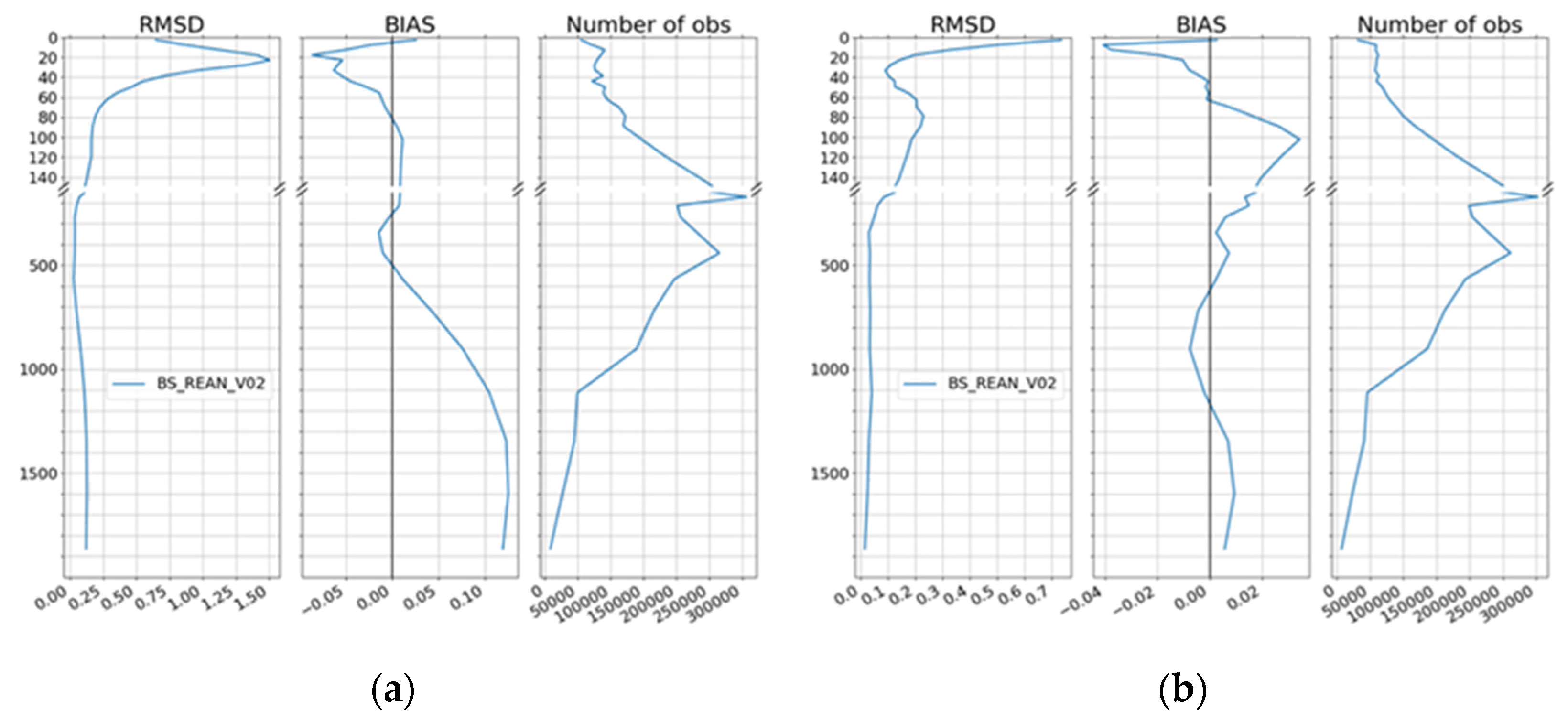
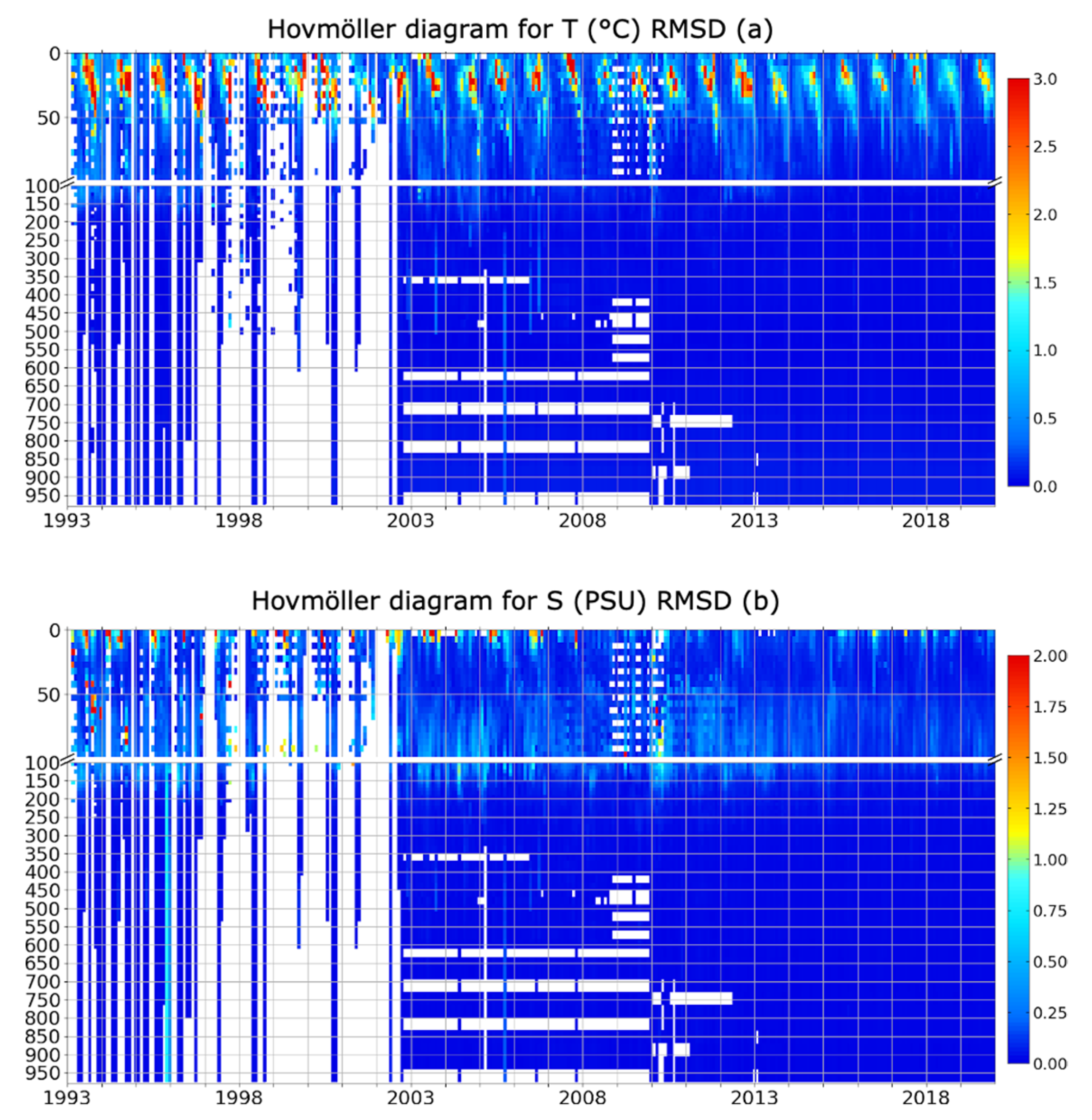
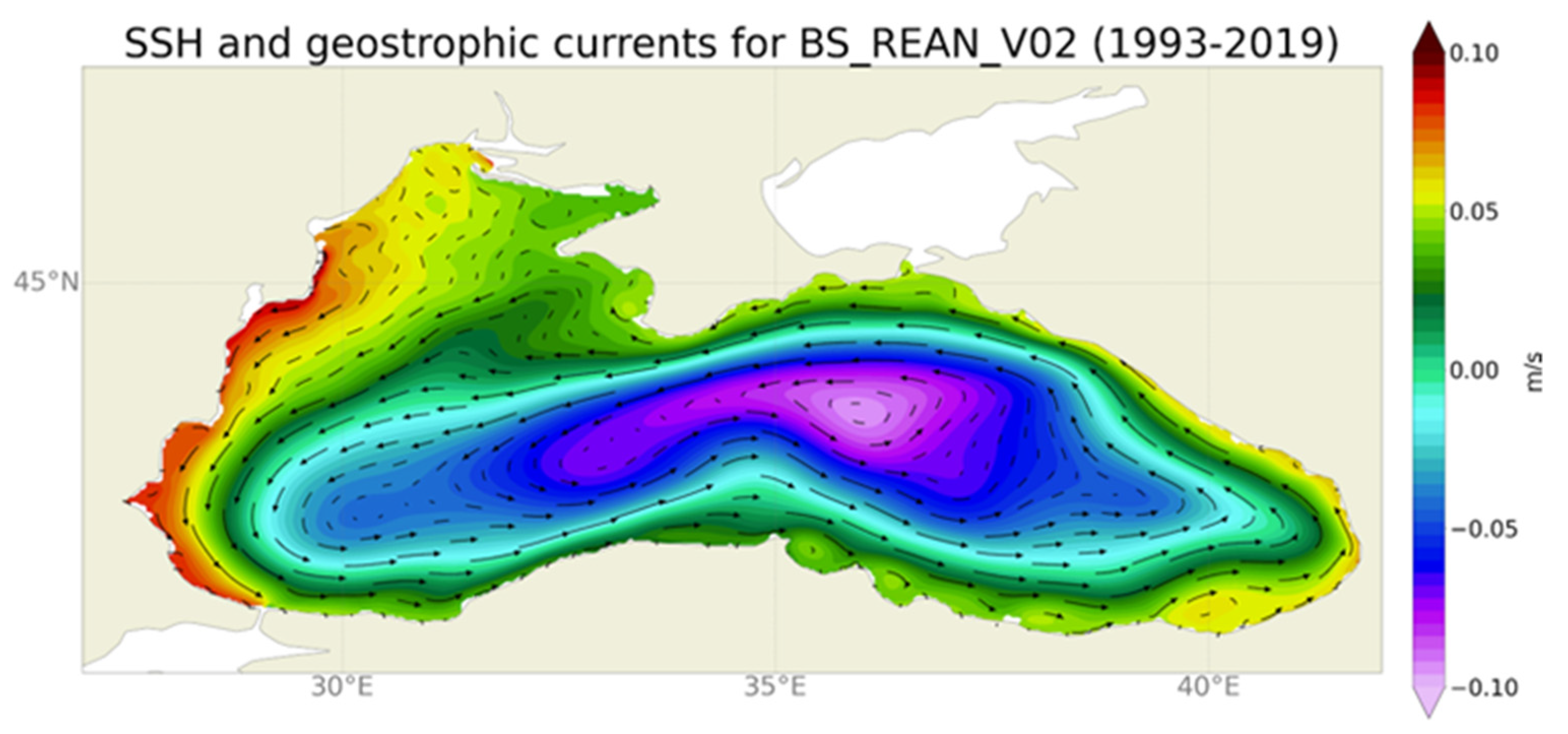
3.1. Validation of BS-PHY Systems

Estimated accuracy numbers (EANs) for BS-PHY NRT were computed using the daily means analysis fields and compared with available observations (Table 1). Root mean square difference (RMSD) and bias were estimated over the period of 2019–2020.

Table 2. EANs for temperature (°C) in terms of bias and RMSD for 2019–2020, including number of observations used in the comparison.

	2019			2020
Layer (m)	Bias	RMSD	N. Observations	Bias	RMSD	N. Observations
5–10	−0.13	1.11	1844	−0.05	0.78	2541
10–20	−0.04	1.87	3462	−0.23	1.57	4217
20–30	0.05	1.62	3484	−0.02	2.10	3925
30–50	0.04	0.91	6909	0.11	1.37	7367
50–75	0.01	0.3	8717	−0.02	0.72	8955
75–100	−0.02	0.17	8329	−0.3	0.27	7647
100–200	0.04	0.09	20,965	0.00	0.10	15,698
200–500	−0.02	0.04	39,114	−0.03	0.05	29,148
500–1000	−0.01	0.02	33,457	−0.01	0.02	18,786

and

Table 3. EANs for salinity (PSU) in terms of bias and RMSD for 2019–2020, including number of observations used in the comparison.

	2019			2020
Layer (m)	Bias	RMSD	N. Observations	Bias	RMSD	N. Observations
5–10	−0.08	0.30	1844	−0.06	0.32	2541
10–20	−0.05	0.25	3462	−0.07	0.25	4217
20–30	0.00	0.23	3484	−0.04	0.22	3925
30–50	0.09	0.29	6909	0.05	0.25	7367
50–75	0.08	0.38	8717	0.14	0.38	8955
75–100	0.02	0.37	8329	0.04	0.40	7647
100–200	−0.02	0.22	20,965	0.01	0.20	15,698
200–500	0.00	0.08	39,114	0.00	0.08	29,148
500–1000	0.00	0.02	33,457	−0.01	0.03	18,786

show EANs computed in the period of 2019–2020 for temperature and salinity, respectively, using ARGO in situ profiles. The evaluation was performed in specific layers. Table 2 shows the averaged RMSD for temperature, which ranges from a maximum of 2.1 °C at 20–30 m to below 0.55 °C for depths greater than 75 m. The temperature bias is around zero over the water column. Regarding salinity (Table 3), the error is approximatively 0.26 PSU in the 5–50 m layer, and then increases to about 0.4 PSU in the halocline. Below 200 m, it is less than 0.1 PSU. Salinity bias is generally slightly negative on the subsurface, but never greater than 0.2 PSU. Regarding sea level, the system has an overall error of about 2.9 cm, while for sea surface temperature, the error is about 0.54 °C [6]. In order to highlight how BS-PHY NRT reproduces the main features of the circulation at the basin scale, Figure 3 and Figure 4 show surface currents as the mean in 2019 and 2020, respectively.

Both figures show the persistency of the Rim current and submesoscale eddies during the selected period—major eddies in the Western basin, the central cyclonic gyre particularly evident in 2020 and less pronounced in 2019, small coastal eddies, and bifurcation of the Rim along the Crimean peninsula. The full overview of the skills is also operationally available through the CMEMS Product Quality Dashboard https://pqd.mercator-ocean.fr/ (accessed on 11 October 2021). Additionally, BS-PHY uses a regional validation website (https://bsfs.cmcc.it/, accessed on 11 October 2021) to evaluate and monitor the quality of the near-real-time physical products.

In the BS-PHY MY, the highest temperature RMSDs are at the seasonal thermocline depths of around 20 m as the values exceed 1.5 °C (Figure 5a). The temperature bias is satisfactory, with a maximum absolute value of about 0.07 °C at the surface, and around zero from 60 down to 500 m, then it increases up to 0.12 °C below 500 m. Salinity has the largest RMSD on the surface, with a maximum of 0.7 PSU (Figure 5b). Similar to the temperature, salinity RMSDs are relatively high at the halocline depths. The Hovmöller diagram of temperature RMSD reveals a clear seasonal pattern: the values are low (high) in winter (summer) so that the highest errors are in the seasonal thermocline (Figure 6a). The Hovmöller diagram of salinity RMSD shows that there is a seasonal signal in the error on the surface: RMSD exceeds 1.5 PSU near the surface before 2008. At depths of 50–150 m, the error decreases up to around 0.8 PSU; however, it is almost zero below 150 m (Figure 6b).

The Hovmöller diagrams reveal the lack of in situ observations between 1997 and 2003 in the Black Sea, which means that for many years the reanalysis system was only constrained by altimeter observations. In comparison with along-track sea level anomaly observations, BS-PHY MY product had a mean sea level anomaly RMSD of 2.24 cm from 1993 to 2019. Finally, the geostrophic currents estimated from the time-averaged sea level (1993–2019) reveal the Rim current, which surrounds the entire Black Sea and forms a large-scale cyclonic gyre (Figure 7). Major details are provided in [47].

3.2. Validation of BS-BIO Systems

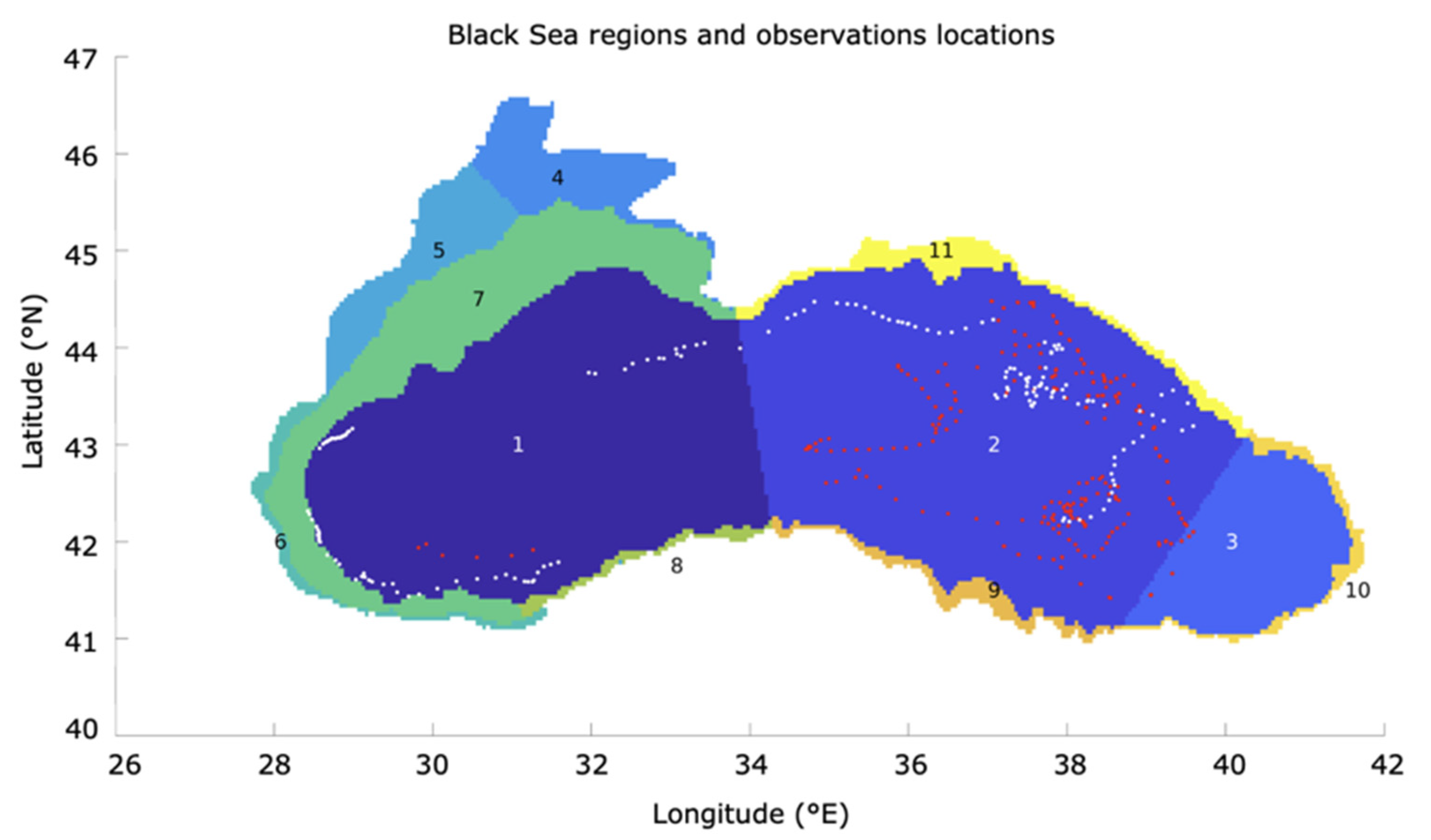
The quality of the BS-BIO NRT and BS-BIO MY systems was assessed using all the observations available for the Black Sea in existing databases (e.g., CMEMS INS and OC TACs, World Ocean database [48], EMODnet at https://portal.emodnet-physics.eu/ (accessed on 11 October 2021), R/V KNORR at https://www.whoi.edu/multimedia/r-v-knorr/, accessed on 11 October 2021) using EANs in the form of BIAS_log10 between the model (M) and the observation (O), as follows (Table 4):

$${\mathrm{BIAS}}_{\log 10}=\log 10\left(\mathrm{M}\right)-\log 10\left(\mathrm{O}\right),$$

(1)

Table 4. BIAS_log10 statistics for chlorophyll obtained for BS-BIO NRT, considering the observation minus model prediction pairs for the various regions (1–11) shown in Figure 8 Data are from the L3 CMEMS satellite chlorophyll observations (Table 1).

Region	1	2	3	4	5	6
EAN	0.012	−0.012	−0.011	0.19	0.15	0.014
	7	8	9	10	11
EAN	0.04	0.009	0.055	0.07	−0.07

Table 4. BIAS_log10 statistics for chlorophyll obtained for BS-BIO NRT, considering the observation minus model prediction pairs for the various regions (1–11) shown in Figure 8 Data are from the L3 CMEMS satellite chlorophyll observations (Table 1).

Region	1	2	3	4	5	6
EAN	0.012	−0.012	−0.011	0.19	0.15	0.014
	7	8	9	10	11
EAN	0.04	0.009	0.055	0.07	−0.07

In the BS-BIO NRT, these error statistics can only be computed for oxygen, chlorophyll, Kd, and PAR, which are derived from satellites and BG-ARGO. Much of the validation has entailed the assessment of the model’s capacity to simulate oxygen. Oxygen integrates the balance of physical and biogeochemical processes such as the formation of the cold intermediate layer, the long-term stability of the main pycnocline, dissolution, photosynthesis, and pelagic and benthic respiration. BS-BIO NRT simulates the main open sea oxycline but overestimates its vertical extension compared to BGC-ARGO data profiles that have a deeper injection of rich oxygen filaments (Figure 9).

In April 2019, the dissolution of oxygen was overestimated, which is probably due to an underestimation of the SST. As shown in Figure 10, on the north-western shelf, the model (in orange) seems to capture the main characteristics of the observed seasonal cycle (in blue), with an oxygenation of the water column in winter due to ventilation and surface photosynthesis, and a reduction later in the year in response to decreased dissolution and the intensification of respiration. The model tends to underestimate the oxygen concentration on the surface in winter time (Jan–Mar) (Figure 10 left), and does the reverse in the bottom layer in summer–autumn time (Jun–Dec), except in winter when the water column is not stratified (Figure 10 right). The model underestimates the oxygenation of the water column in winter, while later in the year, the underestimation of the surface values and the overestimation of the bottom oxygen could indicate an underestimation of the level of primary production. The lower difference between surface and bottom values in the model as compared to the observations suggests excessive mixing in the model. From July to September, the model simulates hypoxia (O₂ < 63 µmol kg⁻¹) in the northernmost part of the shelf; however, the number of hypoxic records is underestimated.

A comparison of the chlorophyll-a (Chla) simulated by BS-BIO NRT and retrieved from the satellite for characteristic optical regions in the Black Sea, as in Figure 8 [50], is shown in Figure 11 (subplots from a to f are related to some crucial regions as shown in Figure 8). Subplots in Figure 11 show that the model reproduces the winter–early spring bloom typical of the deep Black Sea (Figure 11a,c,e) and the higher level of production on the north-western shelf with the presence of several peaks (Figure 11b,d,f). Table 4 shows the log10 BIAS statistics for chlorophyll as the estimated accuracy number (EAN). Considering regions as in Figure 10, EAN is around zero, except in the North-West coastal region (region 4) and at the Danube Delta (region 5), strongly impacted by water discharge (e.g., from the Danube, the Dniepr and the Dniester). Dynamics of the bloom are strongly conditioned by the amount of nutrients discharged on the shelf and the model has the tendency to slightly underestimate the process, as shown by the positive EAN. This is explained using climatological averaged values for the nutrients discharged by the rivers instead of NRT values. The quality of the boundary conditions at the interface with the rivers can hamper model performance.

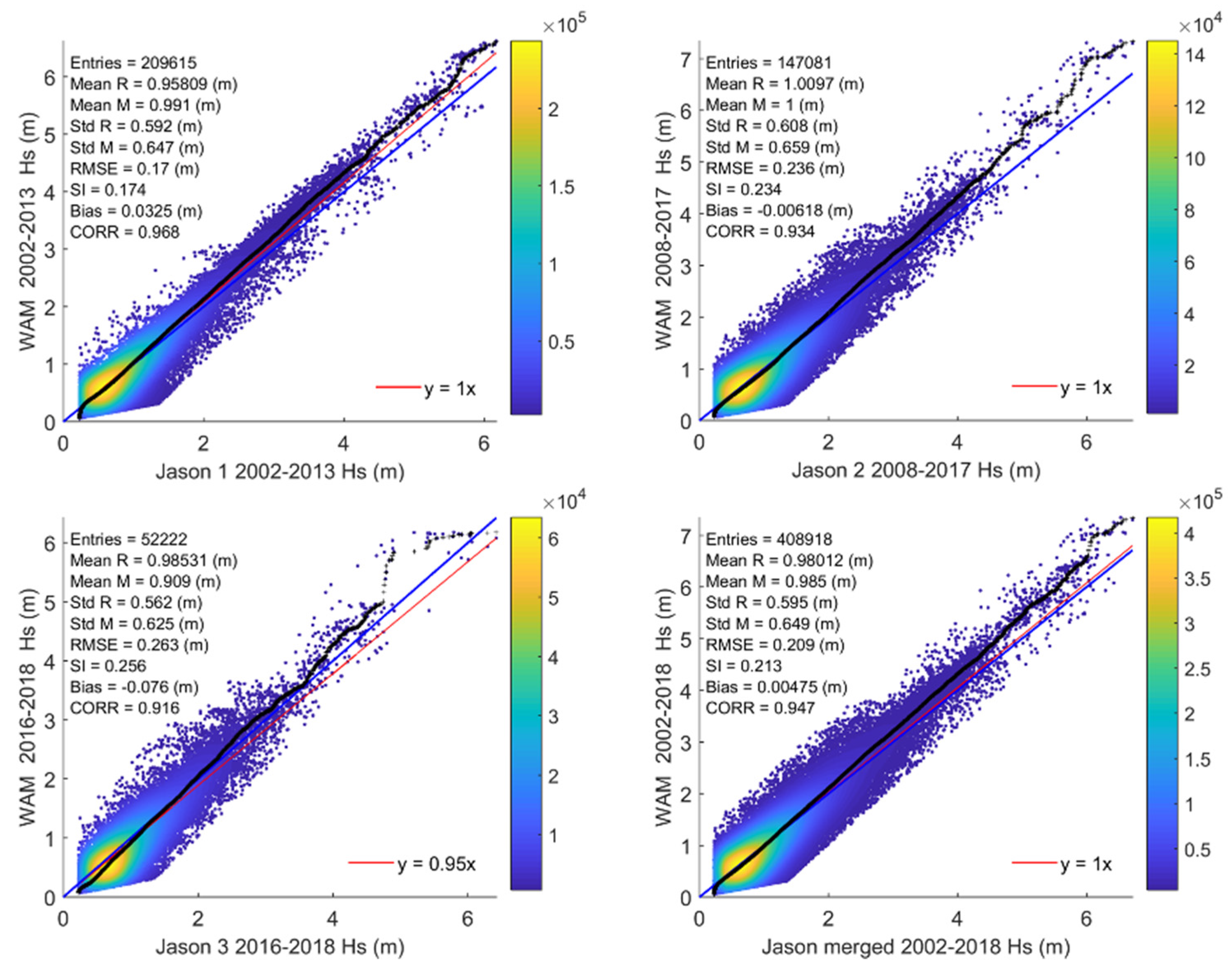
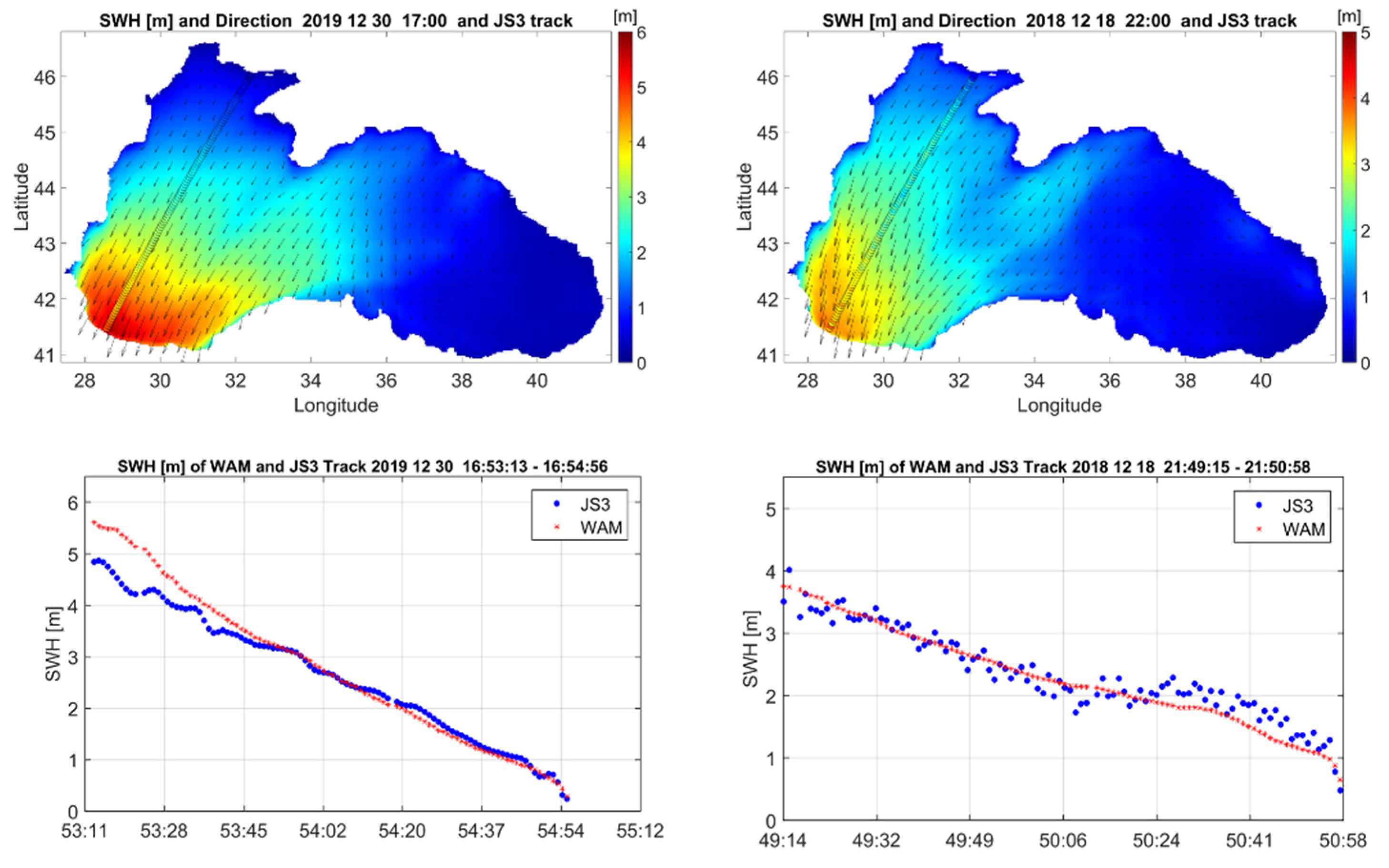
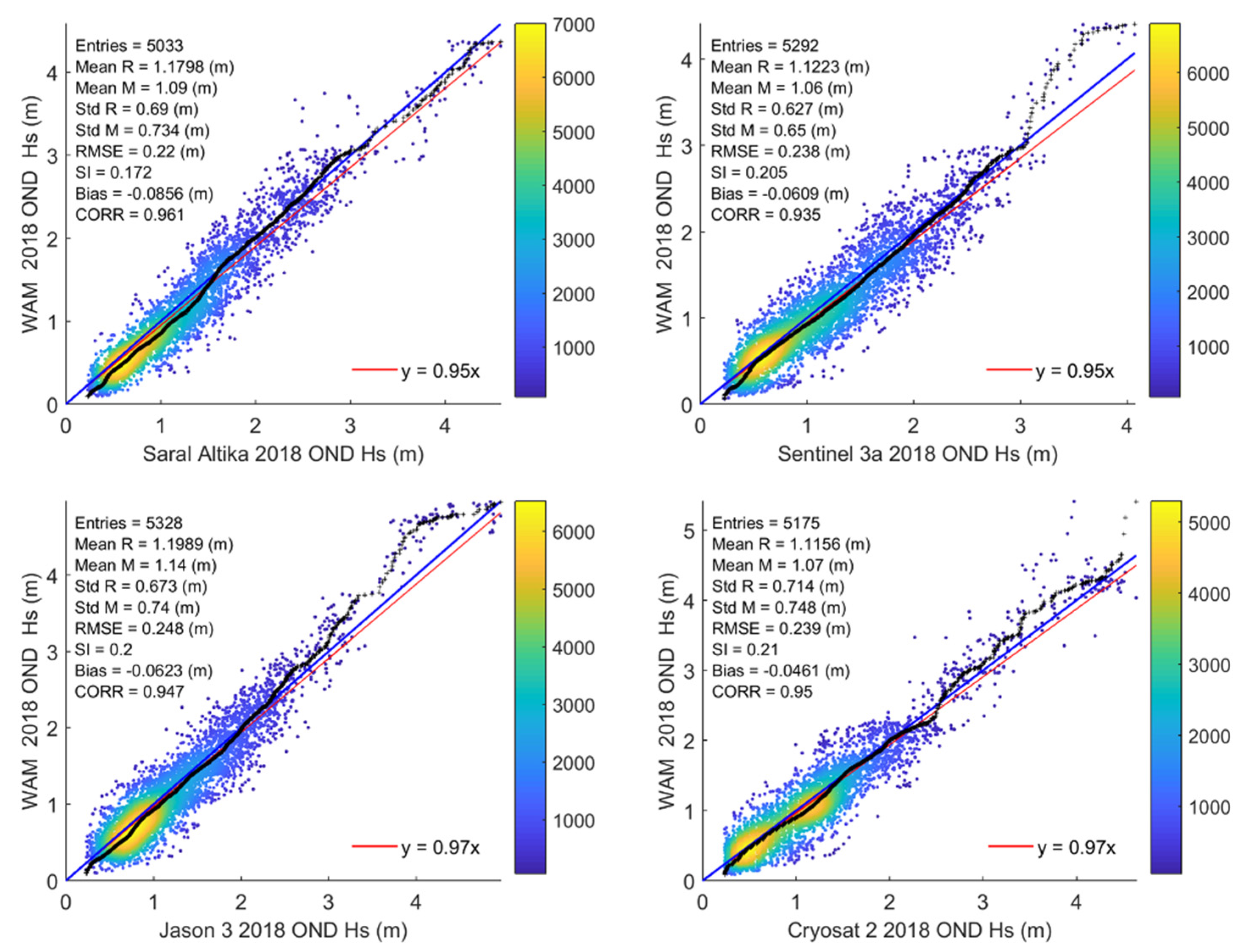
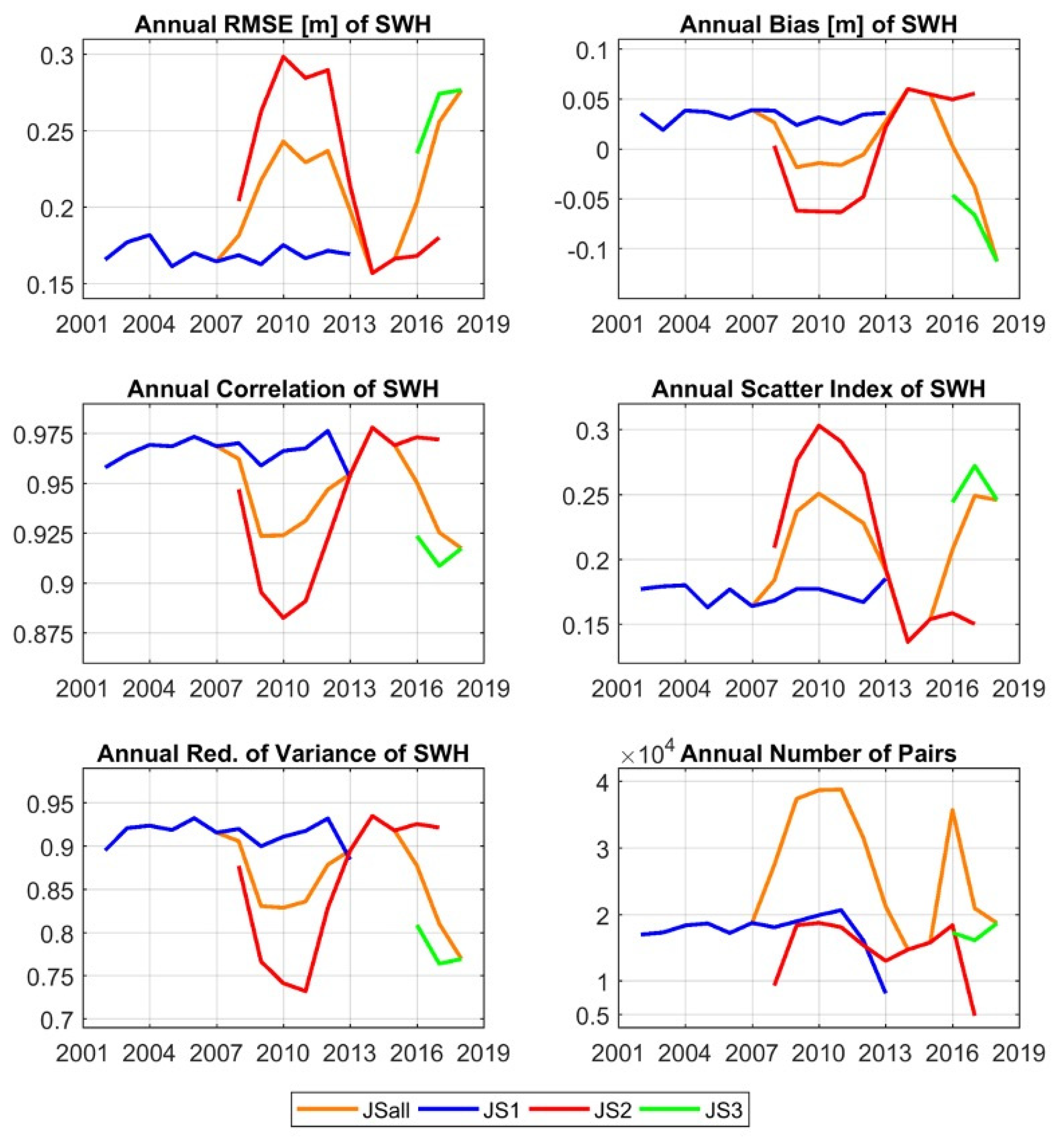
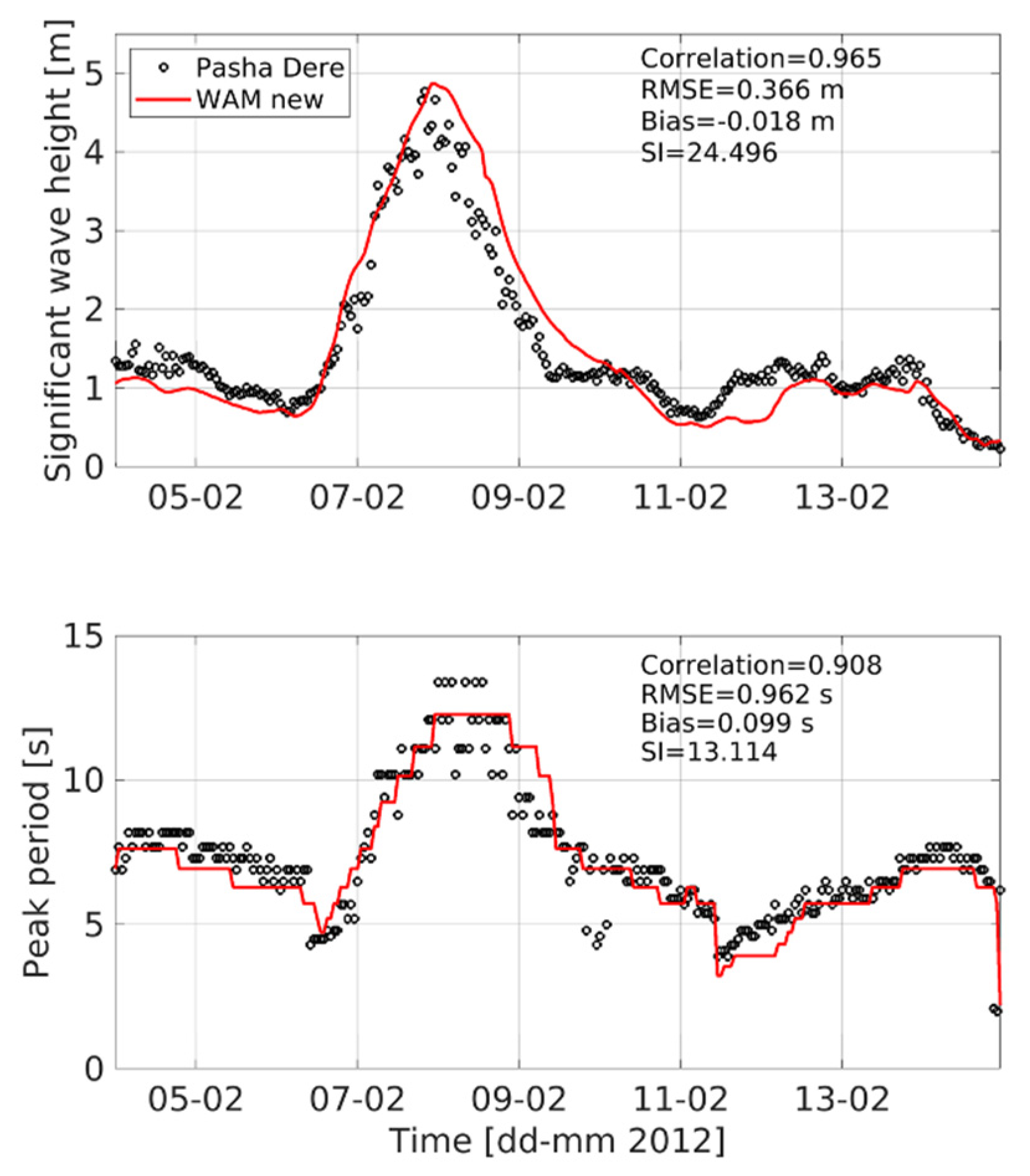
3.3. Validation of BS-WAV Systems

This section describes the quality of the BS-WAV NRT and MY products. Validation is performed by comparing model results with satellite observations, as provided by Sentinel-3a, Sentinel-3b, Cryosat-2, Jason-3, and SARAL/Altika for the period between 01 July 2018 and 30 June 2020, and available in situ observations. The assessment of the corresponding wave hindcast is the best way to understand the validity of the WAM domain model underpinning these products, since the wave analysis-forecast system provided to CMEMS considers surface currents and water-level deviations from BS-PHY NRT. The data are incorporated into the WAM model grid. The growth of errors in the wave forecasts is dominated by growth errors in the forcing fields, which are the 10 m wind fields from the ECMWF IFS (Integrated Forecasting System).

In the new MY product (released to users in December 2020), wave breaking and the assimilation of measured satellite data were taken into account. The required radar altimeter data are available on the public server of AVISO at ftp-access.aviso.altimetry.fr (accessed on 11 October 2021) and CMEMS WAVE TAC, and includes significant wave height and also wind speed. The measured data are assimilated into the wave model fields using an optimal interpolation (OI) scheme. Satellites cross the Black Sea once or twice a day for less than two minutes, so very few measured values are available for assimilation into the wave and wind fields. The currents and water level deviations were not considered for the MYP.

Figure 12 depicts the scatter plots for a comparison between the modelled significant wave height (SWH) (provided by BS-WAV MY) and the one taken from satellites (Jason-1, Jason-2, Jason-3, and combinations thereof). The computed and measured mean values of SWH are generally all located between 0.9 and 1.0 m. The bias is nearly zero for all the merged satellite values, although the values for Jason-2 and Jason-3 show a small underestimation of the wave heights in WAM. The calculated biases of WAM for the different satellites confirm the good agreement between measurements and model results; in fact, they are in the range between −8 cm (Jason-3) and 3 cm (Jason-1). The RMSD varies from 17 cm (Jason-1) to 26 cm (Jason-3). Another deviation is in the difference in the simulated and modelled variability, given as the standard deviations in this article. The differences range from about 5 cm (Jason-2) to 6 cm (Jason-3). Note that the measurement errors and noise that our initial quality control has not filtered out can also impact metrics, thus potentially degrading the model’s skill level. The wind fields also influence the variability and skills of the model as they force the wind-wave model WAM.

Figure 13 shows two examples of a comparison between BS-WAV NRT significant wave height (SWH) and Jason-3 satellite measurements. The figure includes the distribution of SWH combined with a track of the Jason-3 satellite (upper panel), and the corresponding time series of measured and modelled SWH along the satellite track (lower panel).

On the left is the ascending path on 30 December 2019 16:53:13–16:54:56 UTC, which touches the area of the maximum wave height of about 6 m (Figure 13 left). The second example describes the conditions for the path on 18 December 2018 21:49:15–21:50:58 UTC, which crosses the area of maximum wave height of around 4 m (Figure 13 left). Both comparisons show a good agreement between satellite measurements and model results, with a small overestimation by the model for the first example near the maximum SWH. Regarding the quarterly validation procedure for the BS-WAV system, the comparisons between modelled and measured satellite data were analyzed for the two quarters of 2018 and all four quarters of 2019 (

Table 5. EANs for the current BS-WAV NRT system (all values in centimeters).

	Q1/2019		Q2/2019		Q3/2019		Q4/2019		Q1/2020		Q2/2020
Satellite	Bias	RMSD	Bias	RMSD	Bias	RMSD	Bias	RMSD	Bias	RMSD	Bias	RMSD
Saral/Altika	−6.7	16.7	−5.9	16.8	−8.7	16.8	−6.1	21.8	−1.2	24.9	−4.6	16.6
CryoSat-2	−3.2	16.3	−1.1	15.1	−4.0	17.2	2.3	23.7	1.7	25.8	0.5	18.0
Jason-3	−6.4	17.2	−6.0	17.8	−7.2	18.8	−6.2	24.8	−3.9	19.6	−2.8	19.8
Sentinel-3A	−3.4	16.4	−5.4	17.5	−5.9	17.1	−4.7	21.8	−2.2	22.4	−9.6	22.3
Sentinel-3B	−4.1	16.5	−8.0	18.9	−9.5	19.2	−7.4	23.3	−5.4	25.5	−9.6	25.3

). Representative results are shown in Figure 14 for the last quarter of 2018 for the four different satellites SARAL/Altika, Sentinel-3a, Jason-3, and Cryosat-2. The statistics in Table 5 show an underestimation of the measured data by the wave model simulations, particularly revealing a negative bias in the period of 2019–2020.

Figure 15 includes a time series of statistical parameters of the BS-WAV MY product for the complete validation period between 2002 and 2019. On this annual scale, the metrics show that the skill level in all of the statistical parameters varies for the individual satellites. While the values for the bias are always around zero for Jason-1 and Jason-2, the bias for Jason-3 is slightly higher, as shown by the green curve in Figure 15 for the Annual Bias from 2016, and proves the underestimation of 7–10 cm of the measurements by the wave model.

The very good behavior of all statistical parameters for Jason-1 is notable, as there is a very small RMSD value of about 17 cm, a scatter index of about 17%, a correlation of more than 0.96, and a reduction in variance with values above 0.9. That is of course due to the assimilation of Jason-1 data into the wave fields during the time period that they were available.

The parameters for Jason-2 went up for the RMSD (30 cm) around 2010, and down again after 2013 with a low of 17 cm. For the correlation, this is the other way around. The values went down from 0.94 to 0.88 in 2010, and then up again to around 0.97 after 2013. This was expected since after 2013, Jason-2 data were assimilated into the wave fields. The Jason-3 satellite provided data for a short time only. It started in 2016 and showed the most pronounced deviation between model results and the measurements. The RMSD was about 25 cm, the scatter index 25%, and the correlation 0.92. This also generated less satisfactory values for the combined satellite parameters between 2016 and 2019, which were fairly good for the previous years.

Overall, the skill scores depend to some extent on the number of collocated measurements. Clearly, with a decreasing number of observations, the values for the statistical parameters such as RMSD, bias, and scatter index go up, while those for the reduction of variance and the correlation go down. For 11 days, from 4 February 2012 to 15 February 2012, ADCP data were available at the location Pasha Dere (located at 28.03° E, 43.08° N) in the western part of the Black Sea near the Bulgarian coast. This period covers a storm event that occurred between 7 and 9 February 2012. A comparison of the significant wave height and peak period with WAM is shown in Figure 16. The measured and modelled time series of the significant wave height and peak period show a very good agreement. The skill scores support the findings. The bias for the significant wave height is only about −2 cm, while the RMSD is 37 cm. The corresponding values for the peak period, which depend on the resolution of the model frequency, are also very good, with a bias of 0.1 s and an RMSD of about 1 s. The correlation is very high for both integrated parameters: about 0.97 for the significant wave height and 0.91 for the peak period. The peak of the storm was also simulated quite accurately and perfectly illustrates the capacity of the wave model to represent the arrival of a storm as captured by the observations.

4. Summary and Conclusions

The BS-MFC products support users and down-stream services in terms of both sustainable industry and society, by means of accurate datasets, for a number of ocean variables such as temperature, salinity, currents for the physical core, nutrients, phytoplankton, chlorophyll, oxygen for the biogeochemical core, significant wave height and period, Stokes drift, and spectra for the wave core.

Since 2016, the BS-MFC has provided high-quality analyses, 10-day forecasts (as daily and hourly means, including hourly instantaneous for wave fields), and reanalyses (as monthly and daily means from 1993, including hourly predictions for wave fields available from 1979) of the ocean variables to describe the ocean state—both for physics and waves—and biogeochemical processes in the Black Sea region. This is part of the CMEMS product catalogue, available through https://marine.copernicus.eu/ (accessed on 11 October 2021). These systems benefit from constant improvements in the modelling components (e.g., structure, formulation, parameterization) and data assimilation capabilities. BS-MFC has developed reliable interfaces with upstream data providers—ECMWF for atmospheric forcing; CMEMS TACs for access to in situ and satellite observations, including SeaDataNet; EMODnet for historical in situ ones—and the CMEMS Dissemination Unit for the operational delivery of NRT and MY products.

The availability of in situ (i.e., ARGO, mooring stations, radar stations) and satellite observations (i.e., sea surface temperature, sea level anomaly, ocean color, significant wave height, etc.) is fundamental for the evolution of the BS-MFC systems, as reported in [50]. They are used for the performance of validation exercises and data assimilation. Observing capabilities in the Black Sea have significantly improved in recent years, thanks to national and international initiatives such as CMEMS by enforcing Black Sea thematic assembly centers. It is crucial that this effort is maintained in various parts of the sea; for example, in the north-western shelf, which receives vast river inflows, adequate monitoring of physical and biogeochemical variables is needed. BS-MFC models can be used to support the design phase of the observational network and to optimize it by using observing system (simulation) experiments.

In the short term, the BS-MFC implementation phase is going to further improve the overall product offer. The BS-PHY team is building new operational systems based on open boundary conditions at the Marmara Sea to improve the representation of the Bosporus Strait dynamics, including the use of historical data for the Danube River, and increased vertical resolution. BS-BIO plans to improve the data assimilation framework, moving towards ensemble approaches to better represent the uncertainty in the prediction. The BS-WAV team proposes new core models based on WAM Cycle 6.0; the NRT is now one-way offline coupled with hourly means of ocean surface currents and sea levels provided by BS-PHY NRT system. MY now assimilates SWH from SL TAC and, similarly to PHY and BIO, is forced by ECMWF ERA5, with which it will also be coupled in the future.

BS-MFC evolutions are carried out by science-driven activities based on the use of state-of-the-art modelling platforms—NEMO, BAMHBI, and WAM, and data assimilation schemes—devoted to solving physical and biogeochemical processes in an accurate way. For the next generation of BS-MFC systems, research and development efforts will focus on ensemble forecasting, refining the coupling strategy of Ocean-Atmosphere-Waves-Biogeochemistry, developing data assimilation capabilities according to newly-available high-resolution data, developing bio-optical models, and enforcing the optimal interface with the Mediterranean Sea using a high-resolution model for the Marmara Sea, which provides high-quality open boundary conditions for both basins.

References

1. Le Traon, P.Y.; Reppucci, A.; Alvarez Fanjul, E.; Aouf, L.; Behrens, A.; Belmonte, M.; Bentamy, A.; Bertino, L.; Brando, V.E.; Kreiner, M.B.; et al. From Observation to Information and Users: The Copernicus Marine Service Perspective. Front. Mar. Sci. 2019, 6, 234. [Google Scholar] [CrossRef] [Green Version]
2. Pecci, L.; Fichaut, M.; Schaap, D. SeaDataNet, an enhanced ocean data infrastructure giving services to scientists and society. In Proceedings of the IOP Conference Series: Earth and Environmental Science 2020, 11th International Symposium on Digital Earth (ISDE 11), Florence, Italy, 24–27 September 2019; Volume 509. [Google Scholar] [CrossRef]
3. Madec, G.; The NEMO Team. NEMO Ocean Engine; Note du Pole de Modelisation; Institute Pierre-Simon Laplace (IPSL): Paris, France, 2008; ISSN 1288-1619. [Google Scholar]
4. Dobricic, S.; Pinardi, N. An oceanographic three-dimensional variational data assimilation scheme. Ocean. Model. 2008, 22, 89–105. [Google Scholar] [CrossRef]
5. Storto, A.; Dobricic, S.; Masina, S.; Di Pietro, P. Assimilating along-track altimetric observations through local hydrostatic adjustment in a global ocean variational assimilation system. Mon. Weather Rev. 2010, 139, 738–754. [Google Scholar] [CrossRef] [Green Version]
6. Ciliberti, S.A.; Peneva, E.L.; Jansen, E.; Martins, D.; Creti’, S.; Stefanizzi, L.; Lecci, R.; Palermo, F.; Daryabor, F.; Lima, L.; et al. Black Sea Analysis and Forecast (CMEMS BS-Currents, EAS3 System) (Version 1) [Data Set]. Copernicus Monitoring Environment Marine Service (CMEMS). 2020. Available online: https://www.cmcc.it/doi/black-sea-physics-analysis-and-forecast-cmems-bs-currents-eas3-system (accessed on 15 August 2021).
7. Historical GEBCO Data Sets. Available online: https://www.gebco.net/data_and_products/historical_data_sets/#gebco_one (accessed on 11 October 2021).
8. Pettenuzzo, D.; Large, W.G.; Pinardi, N. On the corrections of ERA-40 surface flux products consistent with the Mediterranean heat and water budgets and the connection between basin surface total heat flux and NAO. J. Geophys. Res. Ocean. 2010, 115, C06022. [Google Scholar] [CrossRef]
9. Rosati, A.; Miyakoda, K. A general circulation model for upper ocean simulation. J. Phys. Ocean. 1988, 18, 1601–1626. [Google Scholar] [CrossRef]
10. Adler, R.F.; Huffman, G.J.; Chang, A.; Ferraro, R.; Xie, P.; Janowiak, J.; Rudolf, B.; Schneider, U.; Curtis, S.; Bolvin, D.; et al. The Version 2 Global Precipitation Climatology Project (GPCP) Monthly Precipitation Analysis (1979-Present). J. Hydrometeor. 2003, 4, 1147–1167. [Google Scholar] [CrossRef]
11. Huffman, G.J.; Adler, R.F.; Bolvin, D.T.; Gu, G. Improving the Global Precipitation Record: GPCP Version 2.1. Geophys. Res. Lett. 2009, 36, L17808. [Google Scholar] [CrossRef] [Green Version]
12. Ludwig, W.; Dumont, E.; Meybeck, M.; Heussner, S. River discharges of water and nutrients to the Mediterranean Sea: Major drivers for ecosystem changes during past and future decades? Prog. Oceanogr. 2009, 80, 199–217. [Google Scholar] [CrossRef]
13. Simonov, A.I.; Altman, E.N. Hydrometeorology and Hydrochemistry of the Seas. Vol IV: The Black Sea. Issue 1: Hydrometeorological conditions. Hydrometeoizdat 1991. (In Russian) [Google Scholar]
14. Lima, L.; Aydoğdu, A.; Escudier, R.; Masina, S.; Ciliberti, S.A.; Azevedo, D.; Peneva, E.L.; Causio, S.; Cipollone, A.; Clementi, E.; et al. Black Sea Physical Reanalysis (CMEMS BS-Currents) (Version 1) [Data Set]. Copernicus Monitoring Environment Marine Service (CMEMS). 2020. Available online: https://resources.marine.copernicus.eu/product-detail/BLKSEA_MULTIYEAR_PHY_007_004/INFORMATION (accessed on 15 August 2021).
15. Weatherall, P.; Marks, K.M.; Jakobsson, M.; Schmitt, T.; Tani, S.; Arndt, J.E.; Rovere, M.; Chayes, D.; Ferrini, V.; Wigley, R. A new digital bathymetric model of the world’s ocean. Earth Space Sci. 2015, 2, 331–345. [Google Scholar] [CrossRef]
16. Gürses, Ö. Dynamics of the Turkish Straits System. A Numerical Study with a Finite Element Ocean Model Based on an Unstructured Grid Approach. Ph.D. Thesis, Middle East Technical University, Mersin, Turkey, 2016. [Google Scholar]
17. Aydoğdu, A.; Pinardi, N.; Özsoy, E.; Danabasoglu, G.; Gürses, Ö.; Karspeck, A. Circulation of the Turkish Straits System under interannual atmospheric forcing. Ocean Sci. 2008, 14, 999–1019. [Google Scholar] [CrossRef] [Green Version]
18. Grégoire, M.; Vandenbulcke, L.; Capet, A. Black Sea Biogeochemical Analysis and Forecast (CMEMS Near-Real Time BLACKSEA Biogeochemistry) (Version 1) [Data Set]. Copernicus Monitoring Environment Marine Service (CMEMS). 2020. Available online: https://resources.marine.copernicus.eu/product-detail/BLKSEA_ANALYSIS_FORECAST_BIO_007_010/INFORMATION (accessed on 15 August 2021).
19. Grégoire, M.; Vandenbulcke, L.; Capet, A. Black Sea Biogeochemical Reanalysis (CMEMS BS-Biogeochemistry) (Version 1) [Data Set]. Copernicus Monitoring Environment Marine Service (CMEMS). 2020. Available online: https://resources.marine.copernicus.eu/product-detail/BLKSEA_REANALYSIS_BIO_007_005/INFORMATION (accessed on 15 August 2021).
20. Grégoire, M.; Raick, C.; Soetaert, K. Numerical modeling of the deep Black Sea ecosystem functioning during the late 80’s (eutrophication phase). Prog. Oceanogr. 2008, 76, 286–333. [Google Scholar] [CrossRef]
21. Grégoire, M.; Soetaert, K. Carbon, nitrogen, oxygen and sulfide budgets in the Black Sea: A biogeochemical model of the whole water column coupling the oxic and anoxic parts. Ecol. Model. 2010, 221, 2287–2301. [Google Scholar] [CrossRef]
22. Capet, A.; Meysman, F.J.R.; Akoumianaki, I.; Soetaert, K.; Grégoire, M. Integrating sediment biogeochemistry into 3D oceanic models: A study of benthic-pelagic coupling in the Black Sea. Ocean Model. 2016, 101, 83–100. [Google Scholar] [CrossRef]
23. Soetaert, K.; Hofmann, A.; Middelburg, J.; Meysman, F.; Greenwood, J. The effect of biogeochemical processes on pH. Mar. Chem. 2007, 105, 30–51. [Google Scholar] [CrossRef]
24. Soetaert, K.; Middelburg, J.; Herman, P.; Buis, K. On the coupling of benthic pelagic biogeochemical models. Earth-Sci. Rev. 2000, 51, 173–201. [Google Scholar] [CrossRef]
25. Vandenbulcke, L.; Barth, A. A stochastic operational forecasting system of the Black Sea: Technique and validation. Ocean Model. 2015, 93, 7–21. [Google Scholar] [CrossRef]
26. Kanakidou, M.; Duce, R.A.; Prospero, J.M.; Baker, A.R.; Benitez-Nelson, C.; Dentener, F.J.; Hunter, K.A.; Liss, P.S.; Mahowald, N.; Okin, G.S.; et al. Atmospheric fluxes of organic N and P to the global ocean. Glob. Biogeochem. Cycles 2016, 26, GB3026. [Google Scholar] [CrossRef]
27. Stanev, E.V.; Staneva, J.V.; Roussenov, V.M. On the Black Sea water mass formation. Model sensitivity study to atmospheric forcing and parameterization of physical processes. J. Mar. Syst. 1997, 13, 245–272. [Google Scholar] [CrossRef]
28. Stanev, E.V.; Beckers, J.M. Barotropic and baroclinic oscillations in strongly stratified ocean basins. Numerical study for the Black Sea. J. Mar. Syst. 1999, 19, 65–112. [Google Scholar] [CrossRef]
29. Staneva, J.; Behrens, A.; Ricker, M.; Gayer, G. Black Sea Waves Analysis and Forecast (CMEMS BS-Waves) (Version 2) [Data Set]. Copernicus Monitoring Environment Marine Service (CMEMS). 2020. Available online: https://resources.marine.copernicus.eu/product-detail/BLKSEA_ANALYSISFORECAST_WAV_007_003/INFORMATION (accessed on 15 August 2021).
30. Staneva, J.; Behrens, A.; Ricker, M.; Gayer, G. Black Sea Waves Reanalysis (CMEMS BS-Waves) (Version 2) [Data Set]. Copernicus Monitoring Environment Marine Service (CMEMS). 2020. Available online: https://www.cmcc.it/doi/black-sea-waves-reanalysis-cmems-blk-waves (accessed on 15 August 2021).
31. The WAMDI Group. The WAM Model-A Third Generation Ocean Wave Prediction Model. J. Phys. Oceanogr. 1988, 18, 1775–1810. [Google Scholar] [CrossRef] [Green Version]
32. Staneva, J.; Ricker, M.; Carrasco Alvarez, R.; Breivik, Ø.; Schrum, C. Effects of Wave-Induced Processes in a Coupled Wave-Ocean Model on Particle Transport Simulations. Water 2021, 13, 415. [Google Scholar] [CrossRef]
33. Komen, G.J.; Cavaleri, L.; Donelan, M.; Hasselmann, K.; Hasselmann, S.; Janssen, P.A.E.M. Dynamics and Modelling of Ocean Waves; Cambridge University Press: Cambridge, UK, 1994; 532p. [Google Scholar]
34. Gunther, H.; Hasselmann, S.; Janssen, P.A.E.M. The WAM Model Cycle 4.0. User Manual. Technical Report No. 4; Deutsches Klimarechenzentrum: Hamburg, Germany, 1992; 102p. [Google Scholar]
35. Janssen, P.A.E.M. Progress in ocean wave forecasting. J. Comput. Phys. 2008, 227, 3572–3594. [Google Scholar] [CrossRef]
36. Staneva, J.; Behrens, A.; Wahle, K. Wave modelling for the German Bight coastal-ocean predicting system. J. Phys. Conf. Ser. 2015, 633, 233–254. [Google Scholar] [CrossRef]
37. Staneva, J.; Behrens, A.; Gayer, G. Predictability of large wave heights in the western Black Sea during the 2018 winter storms. J. Oper. Oceanogr. 2020, 13. [Google Scholar] [CrossRef]
38. Hersbach, H.; Janssen, P.A.E.M. Improvement of the Short-Fetch Behavior in the Wave Ocean Model (WAM). J. Atmos. Ocean. Technol. 1999, 16, 884–892. [Google Scholar] [CrossRef]
39. Bidlot, J.-R.; Janssen, P.; Abdalla, S. A Revised Formulation of Ocean Wave Dissipation and Its Model Impact; ECMWF Tech. Memo. 509; ECMWF: Reading, UK, 2007; 27p. [Google Scholar]
40. Behrens, A. Development of an ensemble prediction system for ocean surface waves in a coastal area. Ocean Dyn. 2015, 63, 469–486. [Google Scholar] [CrossRef] [Green Version]
41. Staneva, J.; Alari, V.; Breivik, Ø.; Bidlot, J.-R.; Mogensen, K. Effects of wave-induced forcing on a circulation model of the North Sea. Ocean Dyn. 2017, 67, 81–191. [Google Scholar] [CrossRef]
42. Staneva, J.; Grayek, S.; Behrens, A.; Günther, H. GCOAST: Skill assessments of coupling wave and circulation models (NEMO-WAM). In Proceedings of the Journal of Physics: Conference Series, 9th International Conference on Mathematical Modeling in Physical Sciences (IC-MSQUARE) 2020, Tinos Island, Greece, 7–10 September 2020; Volume 1730, p. 012071. [Google Scholar] [CrossRef]
43. Lewis, H.W.; Castillo Sanchez, J.M.; Siddorn, J.; King, R.R.; Tonani, M.; Saulter, A.; Sykes, P.; Pequignet, A.-C.; Weedon, G.P.; Palmer, T.; et al. Can wave coupling improve operational regional ocean forecasts for the north-west European Shelf? Ocean Sci. 2019, 15, 669–690. [Google Scholar] [CrossRef] [Green Version]
44. Benetazzo, A.; Barbariol, F.; Pezzutto, P.; Staneva, J.; Behrens, A.; Davison, S.; Bergamasco, F.; Sclavo, M.; Cavaleri, L. Towards a unified framework for extreme sea waves from spectral models: Rationale and applications. Ocean Eng. 2021, 219, 108263. [Google Scholar] [CrossRef]
45. Bruciaferri, D.; Tonani, M.; Lewis, H.W.; Siddorn, J.R.; Saulter, A.; Castillo Sanchez, J.M.; Valiente, N.G.; Conley, D.; Sykes, P.; Ascione, I.; et al. The impact of ocean-wave coupling on the upper ocean circulation during storm events. J. Geophys. Res. Ocean. 2021, 126, e2021JC017343. [Google Scholar] [CrossRef]
46. Hernandez, F.; Blockley, E.; Brassington, G.B.; Davidson, F.; Divakaran, P.; Drevillon, M.; Ishizaki, S.; Garcia-Sotillo, M.; Hogan, P.J.; Lagemma, P.; et al. Recent progress in performance evaluations and near real-time assessment of operational ocean products. J. Oper. Oceanogr. 2015, 8, 221–238. [Google Scholar] [CrossRef]
47. Lima, L.; Ciliberti, S.A.; Aydoğdu, A.; Masina, S.; Escudier, R.; Cipollone, A.; Azevedo, D.; Causio, S.; Peneva, E.; Lecci, R.; et al. Climate signals in the Black Sea from a multidecadal eddy-resolving reanalysis. Front. Mar. Sci. 2021. [Google Scholar] [CrossRef]
48. Boyer, T.P.; Baranova, O.K.; Coleman, C.; Garcia, H.E.; Grodsky, A.; Locarnini, R.A.; Mishonov, A.V.; Paver, C.R.; Reagan, J.R.; Seidov, D.; et al. World Ocean Database 2018; NOAA Atlas NESDIS 87. Available online: https://www.ncei.noaa.gov/sites/default/files/2020-04/wod_intro_0.pdf (accessed on 11 October 2021).
49. Kopelevich, O.V.; Sheberstov, S.V.; Sahling, I.V.; Vazyulya, S.V.; Burenkov, V.I. Bio-optical characteristics of the Russian Seas from satellite ocean color data of 1998–2012. In Proceedings of the VII International Conference “Current Problems in Optics of Natural Waters (ONW 2013)”, St. Petersburg, Russia, 10–14 September 2013. [Google Scholar]
50. Palazov, A.; Ciliberti, S.; Peneva, E.; Grégoire, M.; Staneva, J.; Lemieux-Dudon, B.; Masina, S.; Pinardi, N.; Vandenbulcke, L.; Behrens, A.; et al. Black Sea Observing System. Front. Mar. Sci. 2019, 6, 315. [Google Scholar] [CrossRef]
Figure 1. Black Sea spatial domain and bathymetry (in meters).
Jmse 09 01146 g001
Figure 2. BS-MFC high-level architecture operationally implemented within the CMEMS framework since April 2018.
Jmse 09 01146 g002
Figure 3. Surface currents in 2019.
Jmse 09 01146 g003
Figure 4. Surface currents in 2020.
Jmse 09 01146 g004
Figure 5. Vertical profiles of the root mean square deviation (left panel), bias (middle panel), and number of observations (right panel) for (a) temperature (°C) and (b) salinity (PSU) by comparing the reanalysis results with in situ profilers in the Black Sea domain from 1 January 1993 to 31 December 2019.
Jmse 09 01146 g005
Figure 6. Hovmöller diagrams of root mean square difference for temperature in °C (a) and salinity in PSU (b), by comparing the BS-PHY MY results with in situ profilers in the Black Sea domain from 1 January 1993 to 31 December 2019.
Jmse 09 01146 g006
Figure 7. Mean sea-surface height and corresponding mean sea-surface circulation from the BS-PHY MY product evaluated for the period of 1993–2019.
Jmse 09 01146 g007
Figure 8. Sub-regions schematization from [49] used for computing the error statistics for chlorophyll. Regions 1–3 are the “open sea”, regions 4–5 are the North-Western Shelf, and region 7 is located at the shelf break and is considered a transition region between eutrophic and oligotrophic conditions.
Jmse 09 01146 g008
Figure 9. BGC-ARGO (top) and modelled (bottom) vertical profiles of oxygen from 2018 to 2020.
Jmse 09 01146 g009
Figure 10. Seasonal cycle between 1992 and 2019 of the modelled (orange) and observed (blue) oxygen concentrations over the north-western shelf (at depths of 15–80 m) on the surface (left) and at the bottom (right). The number of observations for each month is reported along the X-axis.
Jmse 09 01146 g010
Figure 11. Time series of satellite (in blue) and model (in orange) chlorophyll spatial averages computed for optical characteristic regions as highlighted by [49].
Jmse 09 01146 g011aJmse 09 01146 g011b
Figure 12. Scatter plots showing satellite measurements versus modelled significant wave heights (BS-WAV MY) for 2002–2013 (Jason-1), 2008–2017 (Jason-2), 2016–2018 (Jason-3), and 2002–2018 (all satellites merged). Additionally, the following are presented: the estimated bivariate probability density (colored area), the linear slope-fit regression of modelled and observed wave heights (red line), specific quantiles taken from the empirical cumulative density function (black line), and the diagonal (blue line). Summary statistics and skill scores are also included. R: reference (satellite) data, M: model data.
Jmse 09 01146 g012
Figure 13. Left: distribution of BS-WAV NRT SWH on 30 December 2019 (17:00 UTC) and a Jason-3 satellite track also on 30 December 2019 (16:53:13–16:54:56 UTC). Right: distribution of SWH on 18 December 2018 (22:00 UTC) and a Jason-3 satellite track on 18 December 2018 (21:49:15–21:50:58 UTC).
Jmse 09 01146 g013
Figure 14. Scatter plots as in Figure 10, but for Q4 2018 and four different satellites.
Jmse 09 01146 g014
Figure 15. Yearly values of significant wave height metrics (using the BS-WAV MY system) for the Black Sea derived from individual and combined satellite measurements.
Jmse 09 01146 g015
Figure 16. Significant wave height and peak period from WAM (using the BS-WAV MY system) and from the ADCP station Pasha Dere from 4 to 15 February 2012.
Jmse 09 01146 g016