Modeling of Ship Fuel Consumption Based on Multisource and Heterogeneous Data: Case Study of Passenger Ship

Abstract

In the current shipping industry, quantitative measures of ship fuel consumption (SFC) have become one of the most important research topics in environmental protection and energy management related to shipping operations. In particular, the rapid development of sensor technologies enables multisource data collection to improve the modeling of the SFC problem. To address the features of such heterogeneous data, this paper proposes an integrated model for the estimation of SFC that includes three modules: a multisource data collection module, a heterogeneous data feature fusion module and a fuel consumption estimation module. First, in the data collection module, data related to SFC are collected by multiple sensors installed aboard the ship. Second, the feature fusion module employs a series of moving overlapped frames to merge different frequency data into small frames so that fusion features can be extracted from the heterogeneous data of multiple sources. Finally, in the fuel estimation module, the fusion features provide a novel way to consider the modeling and estimation of SFC as a classical time-series analysis using various machine learning techniques. Experimentally, linear regression (LR), support vector regression (SVR), and artificial neural network (ANN) were employed as the machine learning methods to train SFC models. Compared with the traditional feature extraction method, the accuracy of LR, SVR, and ANN were improved by 8.5, 0.35 and 51.5%, respectively, using the proposed method. The main contribution of this work is to consider the multisource and heterogeneous problem of sensor-based SFC data and propose an integrated model to extract the information of SFC data. Moreover, the experimental results showed that the estimation accuracy can be greatly improved.

1. Introduction

The shipping industry is one of the pillars of the world economy, as more than 80% of world merchandise trade by volume is carried by sea [1]. However, shipping causes a great deal of environmental pollution compared with other modes of transportation, and the carbon dioxide emissions generated account for a large part of total global greenhouse gas emissions [2]. In recent years, the issue of carbon emissions from ship operations has become a focus of many organizations, including the International Maritime Organization (IMO) and most shipping operators. Global carbon emissions from the shipping industry need to be significantly reduced in the future. Meanwhile, fuel costs have become the largest expenditure item in shipping operations, which has also been a topic of many concerned parties and shipping enterprises [3]. Therefore, in the face of rising fuel costs and the need for environmental protection, the IMO, which includes major shipping countries, urgently needs an effective and quantifiable fuel consumption assessment and estimation method to improve ship energy management.

For modeling ship fuel consumption (SFC), many studies have used artificial neural networks (ANNs) to quantify the relationships between the SFC and its influencing factors [4,5,6,7,8,9,10,11]. Leifsson et al. combined physical knowledge with ANN to build a grey-box model [12]. Ioannis et al. combined a type of neural network named long short-term memory (LSTM) with an Elman neural network (ENN) to forecast fuel consumption of passenger ships [13]. Mou et al. conducted a theoretical analysis to ascertain the principal fuel consumption influencing factors and used random forest regression (RFR) to model inland water SFC [14]. Ran et al. also adopted RFR to establish a model of SFC prediction [15]. Gkerekos et al. used several machine learning methods, such as support vector regression (SVR), extra tree regression (ETR) and ANN to model SFC, and found that ANN showed better performance results than ETR and SVR [16]. Yun et al. adopted models such as gradient boosting regression (GBR), RFR, linear regression (LR) and k-nearest neighbor regression [17]. Several studies have considered domain knowledge of fuel consumption to build SFC models. Meng and Du used two experience formulas to model fuel consumption and estimated the formula coefficients using the trust region algorithm [18]. Igor et al. adopted the numeric fitting method for the recorded SFC data [19]. Some researchers used multiple linear regression analysis, ridge regression and Lasso regression to model SFC and obtained excellent experimental results [20,21]. Omer et al. compared Lasso with ridge regression and found that Lasso had a better performance [22]. Bocchetti et al. used maximum likelihood estimation to estimate the experience formula coefficients [23]. Bialystocki and Konovessis applied polynomial regression analysis to depict the relations between SFC and its influence factors, such as speed and wind [24]. With the recent development of sensor technologies, the kinds and amounts of collected SFC data are growing rapidly. However, the existing SFC models, especially those based on machine learning techniques, cannot easily parse such unstructured data. The multisource and heterogeneous characteristics of novel fuel consumption data brings challenges to the data tailoring process and feature extraction.

In order to improve the predictive ability of SFC models, this paper proposes an integrated model that includes three modules: a multisource data collection module, a heterogeneous data feature fusion module and a fuel consumption estimation module. First, in the multisource data collection module, data related to SFC estimation are collected by multiple sensors attached to ships. Second, the heterogeneous data feature fusion module employs a series of moving overlapped frames to merge the different sensor data into small frames, so that common features can be extracted from various sensors with different sampling frequencies in the time domain. Finally, in the fuel consumption estimation module, several machine learning methods, such as LR, SVR and ANN, are adopted to train the SFC models based on the fusion features with an increased accuracy rate of 8.5%, 0.35%, and 51.5% respectively. The main contribution of this paper is to consider the multi-source and heterogeneous problem of sensor-based SFC data and propose an integrated model. This model merged the time domain of various sensors, performed feature extraction to exploit information of SFC data and greatly improved the prediction accuracy. Moreover, the integrated model could enable more sensor-based SFC data to be used in fuel consumption estimation.

The remainder of this paper is structured as follows. Section 2 provides a literature review of SFC data processing methods. Section 3 introduces the proposed model including multisource data collection, heterogeneous feature fusion and modeling of fuel consumption. This is followed by comparative experiments and result discussions in Section 4. Section 5 presents the conclusions.

2. Literature Review

2.1. Advances of SFC Estimation

In recent years, scholars have been committed to the innovative modeling of fuel consumption models, but rarely paid attention to the issue of data processing. In the practice of marine navigation, SFC-related data can be divided into two categories: log-based data and sensor-based data.

2.1.1. Log-Based SFC Data Collection and Modeling

For log-based data, Luan et al. performed outlier elimination with SFC data by considering three outlier types, namely univariate, multivariate and statistical model noises [9]. After data preprocessing, the various influencing factors were combined with different machine learning methods, such as multiple linear regression and multilayer perception artificial neural network, to model SFC estimation. Tayfun et al. removed the abnormal SFC data related to human error [21]. An SVR, tree-based algorithm, a boosting algorithm, multiple linear regression and ridge regression were used. Ioannis et al. conducted a correlation analysis among SFC influence factors and combined LSTM with ENN to perform SFC predictions [13]. Ran et al. removed the SFC data for speed of less than five knots or no cargo loaded [15]. The RFR was then applied to build the models. With the built model, the navigation speed was optimized subject to minimum fuel consumption and punctual arrival. The experiments showed fuel consumption could be reduced by 2–7% with the proposed methods. Gkerekos et al. removed the recorded anomalies of engine transient data [16]. Domain knowledge was then used to generate new features. For example, forward and aft draught could be transformed into draft amidships and trim. Next, feature standardization was conducted. Processed data were put into various machine learning models to validate the effectiveness of the models. Several other scholars attempted to find a mathematical relationship between fuel consumption and its influencing factors, including draft and displacement. Bialystocki and Konovessis performed three initial corrections to correct recorded SFC data, including draft, weather and hull roughness [24]. Polynomial regression analysis was then adopted to depict the relationships between fuel consumption and speed under different weather conditions. The built SFC model could offer decision support for ship owners and crew members in voyage planning. Igor et al. also conducted noise removal [19]. In order to tackle the problem of nonuniform time SFC data, a moving average was adopted. After data preprocessing, numeric fitting of the recorded data was carried out. Various fitting methods were compared. Lu et al. used an empirical theory to model SFC [25]. Fuel consumption could be obtained from engine load at varying speeds and sea states. Several other investigators provided formulas for SFC modeling. Meng and Du proposed a procedure for outlier removal based on prior domain knowledge [18]. When the changing rate of SFC data did not match the sailing speed and wind force scale, the data points were classified as outliers. In the experiments, the trust region algorithm was used to estimate the parameters of the SFC experience formula. For data processing, Wang et al. conducted Z-scores for all feature vectors [20], then Lasso regression was carried out to estimate formula parameters and implement feature selection to eliminate the high correlations among feature variables. Compared with SVR and ANN, it was found to have better prediction accuracy. Yang et al. used a genetic algorithm (GA) to estimate formula parameters [26]. First, due to shipping companies having specific recording requirements, some information needed for SFC modeling was not recorded and was calculated from known items. GA was then applied to determine the formula parameters and the estimation accuracy was good at the frequent operating conditions of ships.

2.1.2. Sensor-Based SFC Data Collection and Modeling

For sensor-based data, many researchers used ANN to predict SFC. The data of [4] were obtained from an automatic identification system (AIS). First, data normalization was performed to accelerate the convergence of the ANN. The built model was then used to minimize the fuel consumption of a voyage. Petersen took the multisource problem of SFC data into account [5]. The data beyond the frequent operation conditions were regarded as outliers and removed. Windows and feature extraction were then applied to handle asynchronous SFC data. The mean, variance and mean difference were taken as features. Next, the processed data were put into the ANN model to predict fuel consumption. Moreover, Petersen et al. considered several influencing factors such as pitch, sailing speed, trim, draught, and wind [6]. They changed some of the factors, such as pitch and sailing speed, to survey the changing trends of SFC. Ye et al. and Yin et al. also used an ANN model to predict SFC [7,8]. Ye et al. adopted global error and batch gradient descent to train the ANN [7]. Considering that the speed changes sharply during the arrival and departure of ships, Yin and Xu rejected the data for speed less than 15 knots, and normalization was carried out for feature variables [8]. The processed data were then set as inputs to the ANN model. Yin and Xu adopted a dynamic programming (DP) algorithm to optimize the navigation speed with punctual arrival. The experiment results showed that the ship could save 0.71% fuel by following the planned navigation speed. Yasser removed the missing information and noise in raw SFC data with Z-score and Mahalanobis distance for univariate and multivariate noises, respectively [10]. The RFR algorithm was adopted to rank the importance of influencing factors. ANN and multiple regression analysis were performed for SFC modeling. Yun et al. used the GBR, RFR and LR to build a prediction model and discussed two SFC reduction strategies [17]. Moreira used ANN to establish relations between the ship speed and the respective propulsion configuration [11]. Leifsson et al. combined physical knowledge with ANN to generate a grey-box model of SFC estimation, combining the methods either in series or in parallel [12]. For data processing, missing data were removed. The data were then resampled and resolved with a period of 15 s. The experimental results revealed that the prediction accuracy was significantly improved compared with the pure white-box model. Mou et al. applied RFR to SFC prediction [14]. The singular value and noise of the raw SFC data were removed, and the denoised data were numbered and subjected to equidistant sampling and normalization. The processed data were used as input for the RFR. A partial correlation analysis was carried out to survey the importance of different influencing factors. Several researchers have used formulas to depict fuel consumption and estimating formula parameters with some algorithms. Omer et al. applied Lasso and ridge regression and discussed the influence of the penalty factor on the prediction accuracy [22]. Bocchetti et al. used the maximum likelihood estimation algorithm [23]. They carried out variable redefinitions, such as wind direction being transferred into head wind and cross wind. Feature selection was then adopted to ensure appropriate regressors were used for the SFC estimation, and maximum likelihood estimation was used to estimate the regression coefficients. Lokukaluge et al. presented a Gaussian mixture model (GMM) to divide fuel consumption into three clusters, and principal component analysis (PCA) was applied to investigate the impacts of each variable, such as speed, trim and wind [27]. In contrast with SFC prediction, Troden et al. proposed a method to associate fuel consumption with ship operation activities [28]. They used Kalman filters to clear dirty data, such as data when the ship was not underway. According to the changing rate of speed and fuel consumption, the ship operation was divided into different states. Considering the storage and transfer of massive SFC data, Perera and Mo proposed a data compression and recovery system [29]. First, the outliers were removed and normalization was performed. Next, an autoencoder system consisting of PCA was used for data compression. Experiments showed that the fuel data information was well maintained after compression, which offered a way to process SFC data online.

2.2. Limitation of SFC Modeling

It can be noted from the literature that although the structure of log-based data is simple, log- based data cannot describe the fuel consumption situation accurately because of its low sampling frequency compared with sensor-based data. Machine learning methods can greatly improve the estimation accuracy but have a high requirement for the integration of multisensor cross-module heterogeneous data. Therefore, the sensor-based SFC data usually need to be processed by complicated feature extraction methods before use as data for training machine learning models.

Therefore, this study developed an integrated model for SFC estimation:

• Multisource data collection module;
• Heterogeneous data feature fusion module;
• Fuel consumption estimation module.

3. Methodology

3.1. Overview of SFC Estimation

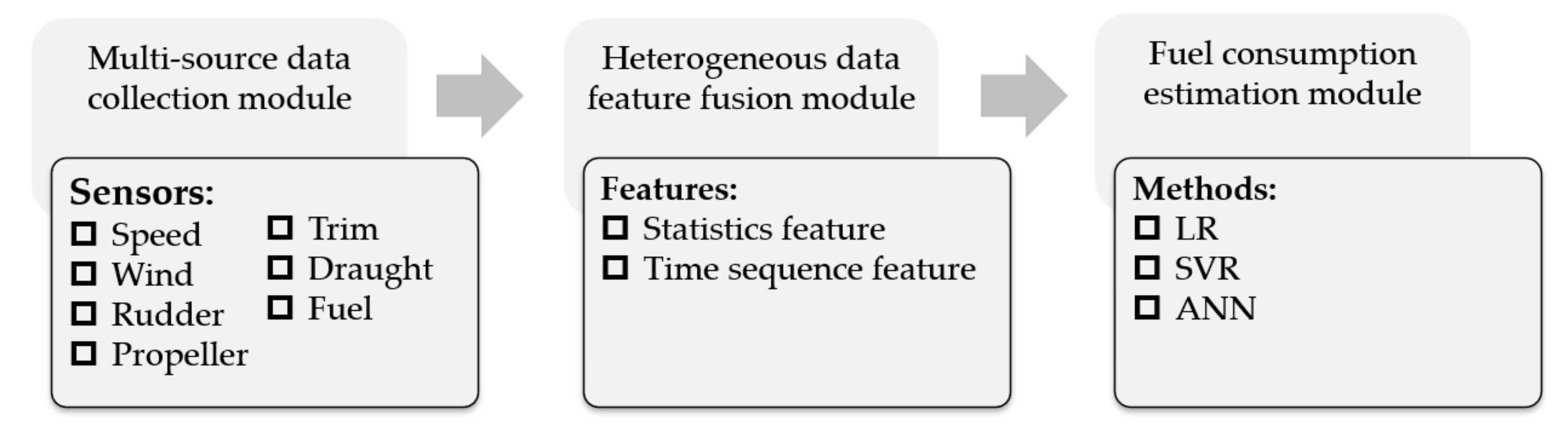
The process of the integrated model is shown in Figure 1. As described, the integrated model consisted of three modules. First, data were collected by multiple sensors. Next, features of heterogeneous data were extracted and fused. Finally, some machine learning methods were adopted to train the SFC mode.

3.2. Multisource Data Collection Module

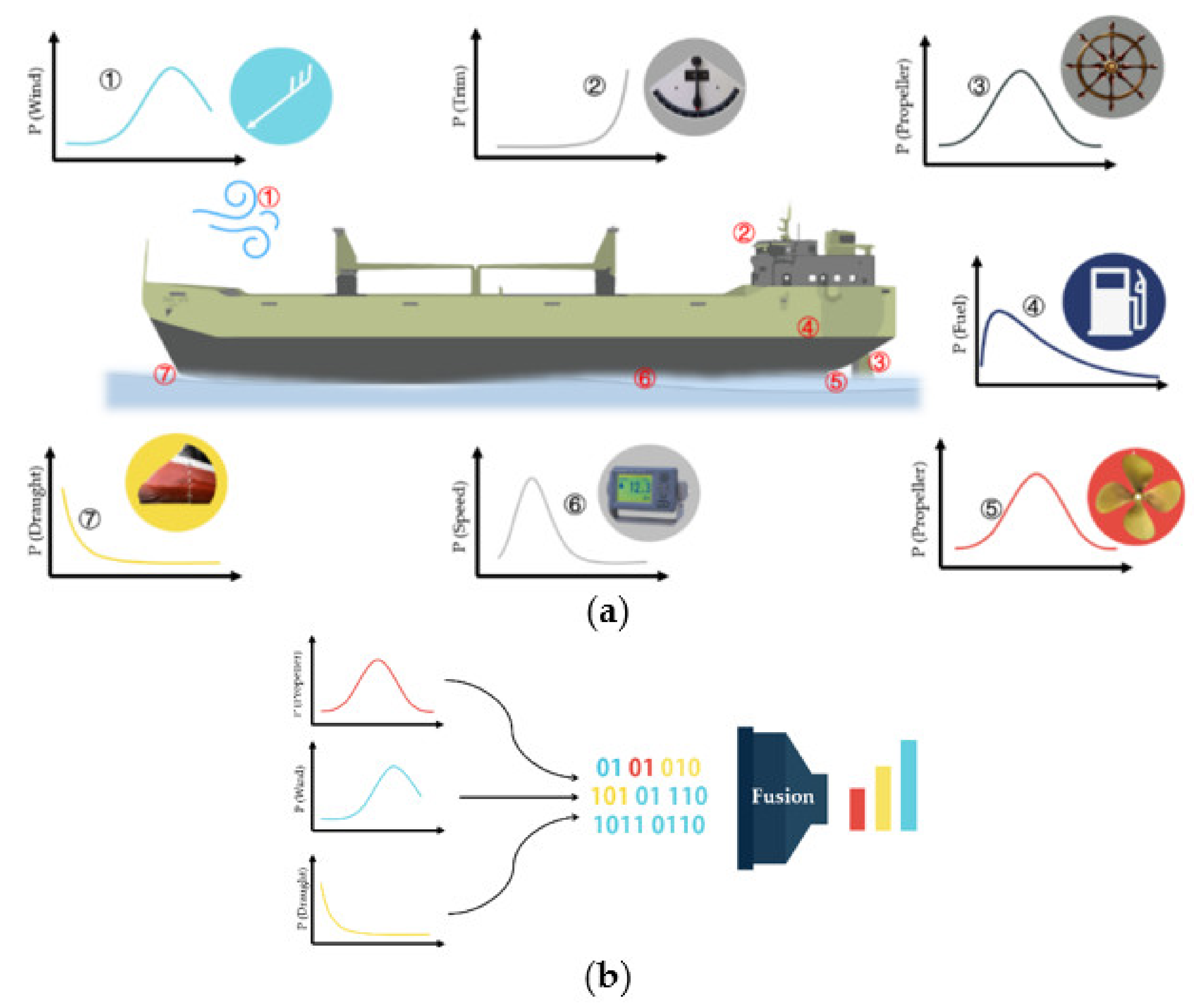
In accordance with the previous literature review, it can be noted that the collection methods of SFC data are mainly divided into log-based data and sensor-based data. Log-based data are filled in by crew members with low sampling frequency. Because it is manually filled in, errors or subjective factors are inevitable, such as the judgment of wind and wave levels. The SFC data and multisource data are collected by multiple sensors installed aboard ships as shown in Figure 2a.

With the rapid development of sensor technologies, multiple types of sensors are installed onboard ships. Much navigation-related information can be precisely measured and obtained. These sensor-based data are closely correlated with the SFC estimation. For instance, the propeller pitch can affect the thrust efficiency and the speed through water. The speed through water goes with SFC. The draught and trim angle indicates the loading conditions of the vessel, which can affect the ship’s water resistance. Therefore, these sensor-based data are important and useful for SFC estimation. However, owing to the different sampling frequencies of various sensors, the collected data are unstructured and heterogeneous, which impedes data processing and utilization. In order to deal with such heterogeneous data, feature extraction and fusion were carried out as shown in Figure 2b.

3.3. Heterogeneous Data Feature Fusion Module

3.3.1. Data Framing

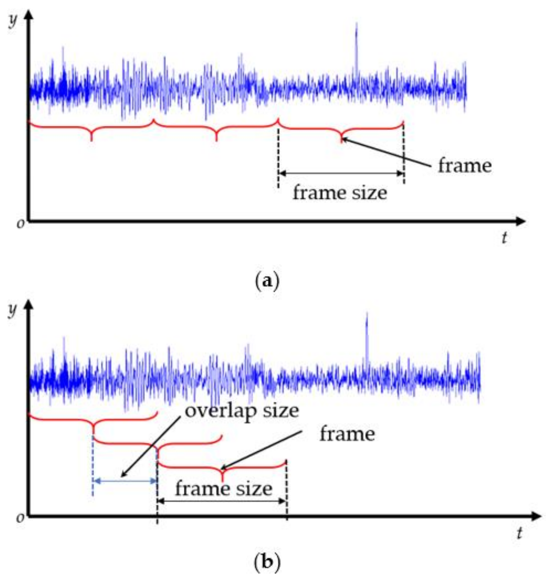
Because the sampling frequency of various sensors is different, the data are not unified in time domain. To unify the time domain of different sensors, the method of framing was adopted. After framing, the frame was set as a new time unit. For framing methods, the traditional way is a nonoverlapped frame [5] without considering the continuity of time series data, as shown in Figure 3a. This study adopted a moving overlapped frame to maintain the continuity of time series data, as shown in Figure 3b.

Using a moving overlapped frame, the processed data have an overlap section between two adjacent frames, which maintains the coherence of the time series data.

3.3.2. Feature Extraction

The input dimension of machine learning methods is usually set as a constant. However, the amount of data for different types of sensors was not constant in a frame. To solve this problem, common features were extracted for different types of sensor data in a frame. The well-extracted features provide more information for SFC estimation. Previous research has mainly extracted the statistical features such as mean, variance and mean difference (MVD). The mean value can indicate the average intensity of data, variance reflects changing magnitude, and mean difference gives the variation tendencies [5]. In this paper, two feature extraction methods are proposed.

(i) Statistics features

Two types of statistical features are used in this paper: statistics feature A (SF. A) comprising mean, variance, mean difference, mode and median; statistics feature B (SF. B) comprising lower margin (Min), lower quartiles (Q₁), median, upper quartile (Q₃), and upper margin (Max).

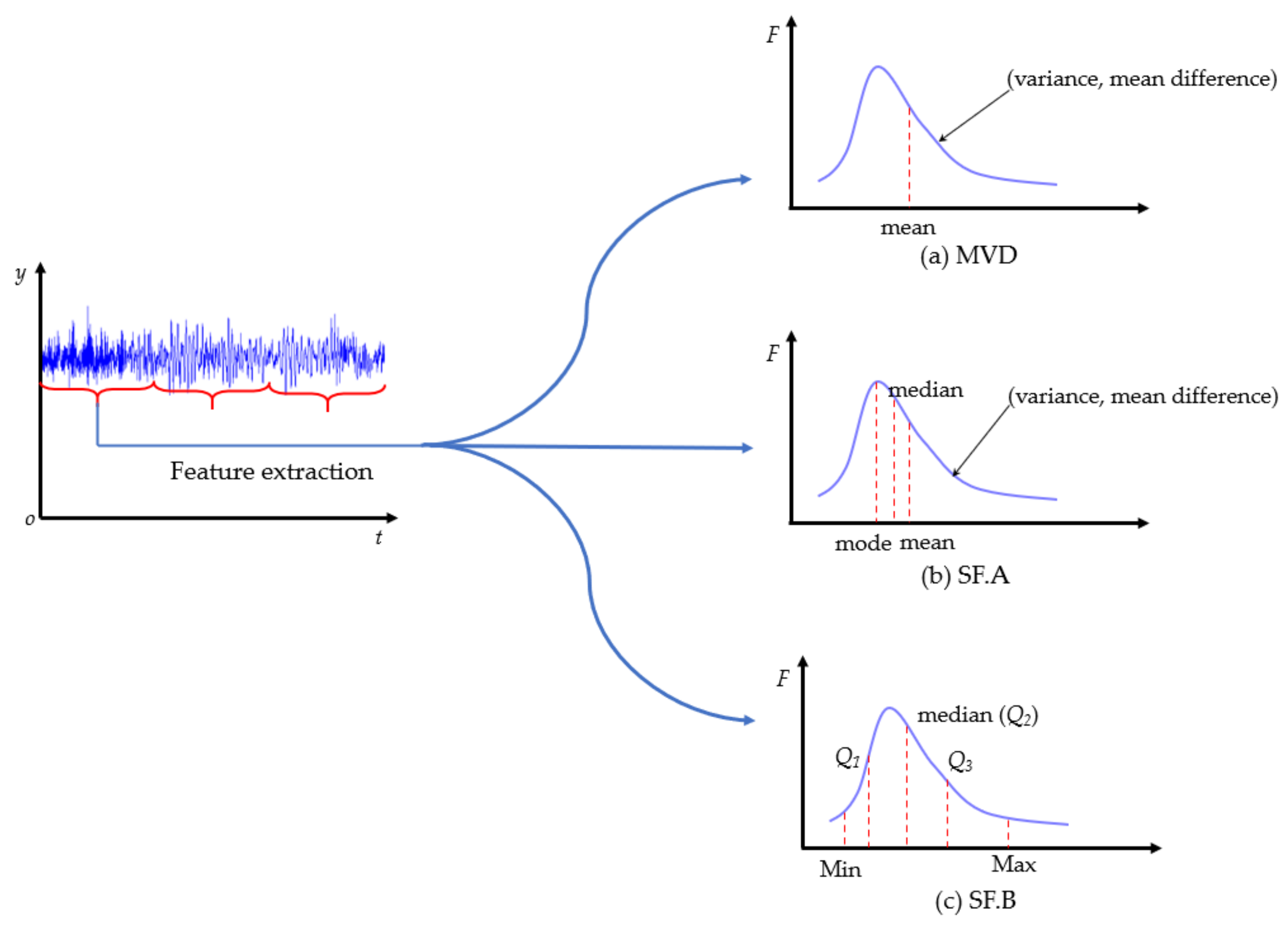
The feature extraction adopted in [5] is the mean, variance and mean difference of data in a frame as shown in Figure 4a. The calculation formulas are shown in Equations (1–3). The variables x and m are data value and data size, respectively, and t is the time step of the sampled points. I is the interval of frames. However, when the data in the frame do not strictly satisfy the normal distribution, these three values are not sufficient to describe the characteristics of data in a frame. For instance, when the data in the frame were left-skewed or right-skewed, even though the mean was the same, the distributions were completely different.

$$Mean\left(I\right)=\frac{1}{m}{\displaystyle \sum }_{i=0}^m{x}_i$$

(1)

$$Variance\left(I\right)=\frac{1}{m}{\displaystyle \sum }_{i=0}^m{\left(x_i-Mean\left(I\right)\right)}^2$$

(2)

$$Mean difference\left(I\right)=\frac{1}{m-1}{\displaystyle \sum }_{i=1}^m\frac{x_i-x_{i-1}}{\Delta t},\hspace{1em}\Delta t=t_i-t_{i-1}$$

(3)

Therefore, mode and median were introduced. The median and mode could be used to reflect the skewed distribution of data in the frame. The mean, variance, mean difference, mode and median of frame data were extracted as SF. A, as shown in Figure 4b.

The extraction steps of SF. A are listed as follows:

(1) Divide the sensor data into frames. Data from different sensors were divided into different sensor frames.

(2) Calculate mean, variance, mean difference, mode and median of data in the respective sensor frame.

(3) Use the mean, variance, mean difference, mode and median as the SF. A of the data in the sensor frame.

For feature extraction, the principal characteristics of the data were extracted in a frame. The mean and variance of SF. A could be easily affected by outliers in the frame. Therefore, SF. B was introduced as shown in Figure 4c. Min, Q₁, median, Q₃ and Max were adopted as SF. B [30]. Data larger than Max or smaller than Min were treated as outliers in each frame.

The extraction steps of SF. B are listed as follows:

(1) Divide the sensor data into frames. Data from different sensors were divided into different sensor frames.

(2) Sort the data in the respective sensor frame according to the data value. Find the median, Q₃ and Q₁ of the data.

(3) Calculate the inter-quartile range, IQR= Q₃-Q₁.

(4) Calculate Max and Min of the data in the sensor frame. Min = Q₁ − 1.5IQR; Max = Q₃ + 1.5IQR.

(5) Use Min, Q₁, median, Q₃, Max calculated above as the SF. B of the data in the sensor frame.

(ii) Time sequence feature (TSF)

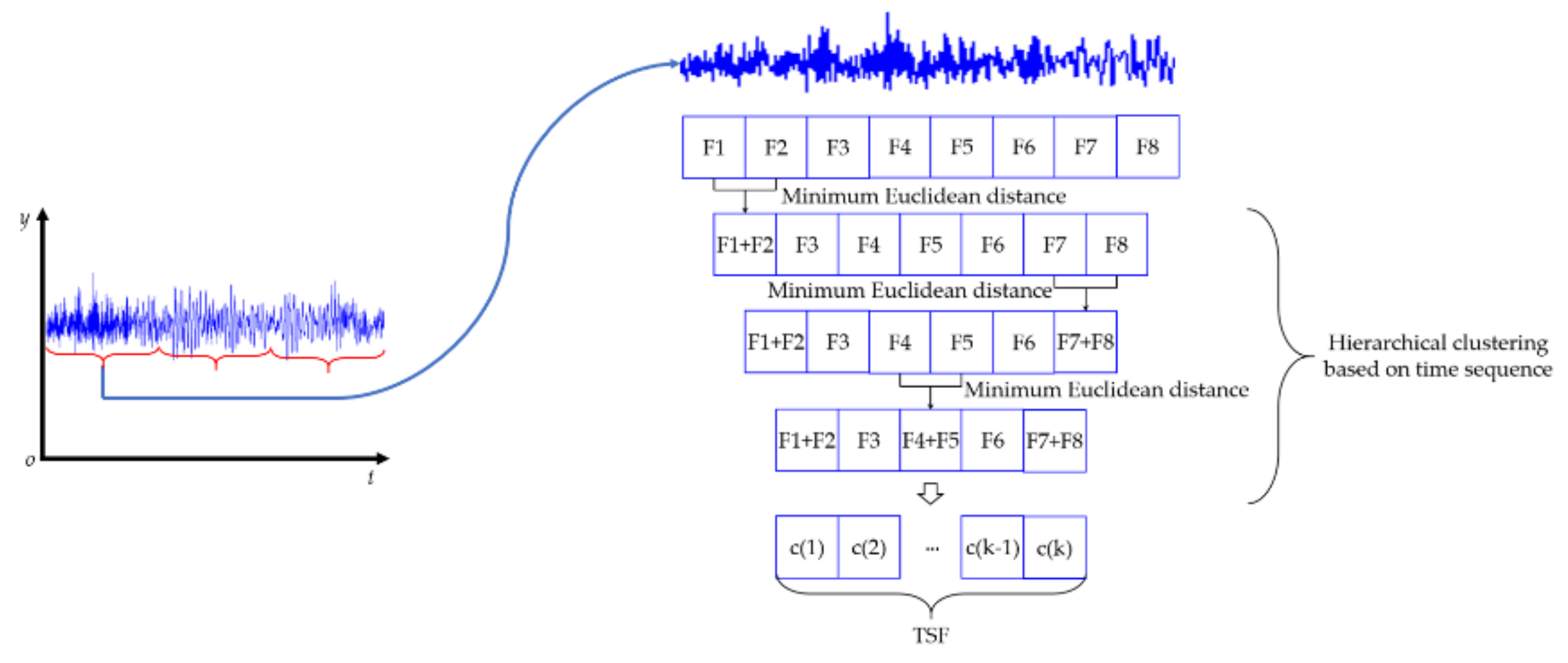
The prementioned statistics feature only considered the distribution of the data. However, the collected data were time-series data. Therefore, a method for extracting TSF was proposed based on hierarchical clustering.

The data value and time step were adopted as clustering attributes to extract the TSF of data in a frame using the following steps. First, the number of TSF points k needs to be set up before hierarchical clustering. Then, the Euclidean distance of every two adjacent sampled points is calculated in the time domain. The two adjacent data points with minimum distance are combined by taking the mean value of those two points. The prementioned process is repeated until the predefined number of feature points k is obtained. The pseudo code for extracting TSF is shown in Algorithm 1.

Algorithm 1 Time Sequence Feature (TSF) extraction

Input: d (data in a frame), k (number of feature points)

Output: TSF

1: epoch=length(d)-k

2: for i=1 to epoch do

3:  for j=1 to length(d) do

4:   dis(j)=dist(d(j), d(j+1))

5:  end for

6:  minidx=Min(dis)

7:  d(minidx)=(d(minidx)+d(minidx+1))/2

8:  delete(d(minidx+1))

9: end for

After applying the TSF extraction algorithm, a series of centers, c₁, c₂, …, c_k, were obtained as shown in Figure 5. These cluster center rankings in time order expressed the time sequence characteristics of the data in the frame. These values c₁, c₂, …, c_k were adopted as the TSF.

3.3.3. Data Structure and Feature Fusion

In the previous section, SFC-related data were collected. Considering that the time domain of these sensors was not unified, framing and feature extraction were applied. Two types of feature extraction methods were proposed, statistical features and TSF. In this section, data structure and fusion features were are presented.

(i) Data structure

In this section, the input and output matrices of the SFC models are introduced. As shown in Equation (4), this integrated model tries to find a relationship f between input matrix X and the output matrix Y. The influence factors of the $i_{th}$ frame were adopted to predict the SFC of the ${\left(i+1\right)}_{th}$ frame.

$$X=\left[\begin{array}{c}{x}_1\\ x_2\\ ⋮\\ x_i\\ ⋮\\ x_{l-1}\end{array}\right],\hspace{1em}\hspace{1em}\hspace{1em}Y=\left[\begin{array}{c}{y}_2\\ y_3\\ ⋮\\ y_{i+1}\\ ⋮\\ y_l\end{array}\right],\hspace{1em}\hspace{1em}\hspace{1em}Y=f\left(X\right)$$

(4)

$$x_i=\left\{s{(1)}_i,\cdots ,s{(j)}_i,\cdots ,s{(m)}_i\right\}$$

(5)

For the $i_{th}$ frame, m types of SFC-related information were collected by m sensors installed on board ships as shown in Equation (5).

For every sensor’s $i_{th}$ frame, the feature extraction algorithm was applied to obtain the data feature of that frame. The features of m sensors were adopted to represent the $i_{th}$ frame ship status. Then the influence factors $X_i$ were used to estimate the SFC $Y_{i+1}$.

As mentioned previously, two feature extraction methods were proposed. For SF. A, the mean, Var, Dif, Med and Mode of data were extracted for $i_{th}$ frame of every kind of sensor as shown in Equation (6).

$$x_i^{SF.A}=\left\{\begin{array}{c}s{\left(1\right)}_i=\left\{s{\left(1\right)}_i^{mean},s{\left(1\right)}_i^{variance},s{\left(1\right)}_i^{mean difference},s{\left(1\right)}_i^{median},s{\left(1\right)}_i^{mode}\right\}\hfill \\ ⋮\hfill \\ s{\left(j\right)}_i=\left\{s{\left(j\right)}_i^{mean},s{\left(j\right)}_i^{variance},s{\left(j\right)}_i^{mean difference},s{\left(j\right)}_i^{median},s{\left(j\right)}_i^{mode}\right\}\hfill \\ ⋮\hfill \\ s{\left(m\right)}_i=\left\{s{\left(m\right)}_i^{mean},s{\left(m\right)}_i^{variance},s{\left(m\right)}_i^{mean difference},s{\left(m\right)}_i^{median},s{\left(m\right)}_i^{mode}\right\}\hfill \end{array}\right.$$

(6)

Considering the effect of outliers in sensor frame, the SF. B was proposed. Min, Q₁, Med, Q₃ and Max were extracted as SF. B as shown in Equation (7).

$$x_i^{SF.B}=\left\{\begin{array}{c}s{\left(1\right)}_i=\left\{s{\left(1\right)}_i^{Max},s{\left(1\right)}_i^{Q_3},s{\left(1\right)}_i^{median},s{\left(1\right)}_i^{Q_1},s{\left(1\right)}_i^{Min}\right\}\hfill \\ ⋮\hfill \\ s{\left(j\right)}_i=\left\{s{\left(j\right)}_i^{Max},s{\left(j\right)}_i^{Q_3},s{\left(j\right)}_i^{median},s{\left(j\right)}_i^{Q_1},s{\left(j\right)}_i^{Min}\right\}\hfill \\ ⋮\hfill \\ s{\left(m\right)}_i=\left\{s{\left(m\right)}_i^{Max},s{\left(m\right)}_i^{Q_3},s{\left(m\right)}_i^{median},s{\left(m\right)}_i^{Q_1},s{\left(m\right)}_i^{Min}\right\}\hfill \end{array}\right.$$

(7)

To extract the time sequence characteristics of the data in a frame, the TSF feature was proposed based on a hierarchical clustering algorithm. The cluster center $c_1,c_2,\cdots ,c_k$ was adopted as the TSF as shown in Equation (8).

$$x_i^{TSF}=\left\{\begin{array}{c}s{\left(1\right)}_i=\left\{s{\left(1\right)}_i^{c_1},s{\left(1\right)}_i^{c_2},\cdots ,s{\left(1\right)}_i^{c_{k-1}},s{\left(1\right)}_i^{c_k}\right\}\hfill \\ ⋮\hfill \\ s{\left(j\right)}_i=\left\{s{\left(j\right)}_i^{c_1},s{\left(j\right)}_i^{c_2},\cdots ,s{\left(j\right)}_i^{c_{k-1}},s{\left(j\right)}_i^{c_k}\right\}\hfill \\ ⋮\hfill \\ s{\left(m\right)}_i=\left\{s{\left(m\right)}_i^{c_1},s{\left(m\right)}_i^{c_2},\cdots ,s{\left(m\right)}_i^{c_{k-1}},s{\left(m\right)}_i^{c_k}\right\}\hfill \end{array}\right.$$

(8)

(ii) Feature fusion

The statistics feature only considered the data distribution in the frame. However, the TSF can also reflect the time sequence characteristics of the data in the frame. Therefore, in this part, different types of features are fused together. For sensor $j=1 to m$, the SF. A and SF. B were fused as shown in Equations (9) and (10).

$$\left\{SF.A,SF.B\right\}=\left\{x_i^{SF.A},x_i^{SF.B}\right\},\hspace{1em}{x}_i^{SF.A}\in SF.A,x_i^{SF.B}\in SF.B$$

(9)

$$\begin{array}{c}s{\left(j\right)}_i^{SF.A,SF.B}=\{s{\left(j\right)}_i^{mean},s{\left(j\right)}_i^{variance},s{\left(j\right)}_i^{mean difference},\\ s{\left(j\right)}_i^{median},s{\left(j\right)}_i^{mode},s{\left(j\right)}_i^{Max},\\ s{\left(j\right)}_i^{Q_3},s{\left(j\right)}_i^{median},s{\left(j\right)}_i^{Q_1},s{\left(j\right)}_i^{Min}\}\end{array}$$

(10)

The statistics feature was combined with TSF for the purpose of considering both the distribution and time sequence characteristics of sensor-based data in the frame. For sensor $j=1 to m$, the SF. A and TSF were fused as shown in Equations (11) and (12). The SF. B and TSF were fused as shown in Equations (13) and (14). Then SF. A, SF. B and TSF were fused together as shown in Equations (15) and (16).

$$\left\{SF.A,TSF\right\}=\left\{x_i^{SF.A},x_i^{TSF}\right\},\hspace{1em}{x}_i^{SF.A}\in SF.A,x_i^{TSF}\in TSF$$

(11)

$$\begin{array}{c}s{\left(j\right)}_i^{SF.A,TSF}=\{s{\left(j\right)}_i^{mean},s{\left(j\right)}_i^{variance},s{\left(j\right)}_i^{meandifference},\\ s{\left(j\right)}_i^{median},s{\left(j\right)}_i^{mode},\\ s{\left(j\right)}_i^{c_1},s{\left(j\right)}_i^{c_2},\cdots ,s{\left(j\right)}_i^{c_{k-1}},s{\left(j\right)}_i^{c_k}\}\end{array}$$

(12)

$$\left\{SF.B,TSF\right\}=\left\{x_i^{SF.B},x_i^{TSF}\right\},\hspace{1em}{x}_i^{SF.B}\in SF.B,x_i^{TSF}\in TSF$$

(13)

$$\begin{array}{r}\hfill {s\left(j\right)}_i^{SF.B,TSF}=\{{s\left(j\right)}_i^{Max},{s\left(j\right)}_i^{Q_3},{s\left(j\right)}_i^{median},{s\left(j\right)}_i^{Q_1},{s\left(j\right)}_i^{Min},\\ \hfill {s\left(j\right)}_i^{c_1},{s\left(j\right)}_i^{c_2},\cdots ,{s\left(j\right)}_i^{c_{k-1}},{s\left(j\right)}_i^{c_k}\}\end{array}$$

(14)

$$\left\{SF.A,SF.B,TSF\right\}=\left\{x_i^{SF.A},x_i^{SF.B},x_i^{TSF}\right\},\hspace{1em}{x}_i^{SF.A}\in SF.A,x_i^{SF.B}\in SF.B,x_i^{TSF}\in TSF$$

(15)

$$\begin{array}{c}s{\left(j\right)}_i^{SF.A,SF.B,TSF}=\{s{\left(j\right)}_i^{mean},s{\left(j\right)}_i^{variance},s{\left(j\right)}_i^{meandifference},s{\left(j\right)}_i^{median}\\ s{\left(j\right)}_i^{mode},s{\left(j\right)}_i^{Max},s{\left(j\right)}_i^{Q_3},s{\left(j\right)}_i^{median},s{\left(j\right)}_i^{Q_1}\\ s{\left(j\right)}_i^{Min},s{\left(j\right)}_i^{c_1},s{\left(j\right)}_i^{c_2},\cdots ,s{\left(j\right)}_i^{c_{k-1}},s{\left(j\right)}_i^{c_k}\}\end{array}$$

(16)

3.4. Fuel Consumption Estimation Module

The fuel consumption estimation was used to interpret the relationships between the influencing factors x $\left\{s\left(1\right),\cdots ,s\left(j\right),\cdots ,s\left(m\right)\right\}$, and the SFC as y. In this module, three machine learning methods were applied to SFC estimation based on the influencing factors x.

3.4.1. LR-Based SFC Estimation

LR provided that the relations between the influencing factors x and SFC y was linear. The hypothesis and cost function of LR could be written as Equations (17) and (18).

$$f\left(x,\theta \right)={\theta }_0\mathrm{\hspace{1em}}+{\theta }_{1}s\left(1\right)+\mathrm{\dots }+{\theta }_{j}s\left(j\right)+\mathrm{\dots }+{\theta }_{m}s\left(m\right)$$

(17)

$$J\left({\theta }_0,{\theta }_1,{\theta }_2,\dots ,{\theta }_{10}\right)=\frac{1}{2m}{\displaystyle \sum }_{i=1}^{m-1}{\left(y_{i+1}-f\left(x_i,\theta \right)\right)}^2$$

(18)

The optimization objective was to find out the parameters ${\theta }_0, {\theta }_1, {\theta }_2,\dots , {\theta }_m$, which could minimize the error between the predicted SFC and real SFC.

3.4.2. SVR-Based SFC Estimation

SVR was extended by a support vector machine (SVM). In SVR, the influencing factors x $\left\{s\left(1\right),\dots ,s\left(j\right),\dots ,s\left(m\right)\right\}$ were mapped into a higher dimensional feature space by a kernel function, $\phi$, as shown in Equation (19). The widely adopted kernel functions were linear kernel, polynomial kernel and radial basis function (RBF) kernel.

$$f\left(x,W\right)=W\phi \left(x\right)+b$$

(19)

$$\left\{\begin{array}{l}\min \frac{1}{2}\parallel W{\parallel }^2\hfill \\ \mathrm{s}.\mathrm{t}. \left|y_{i+1}-f\left(x_i,W\right)\right|\le \epsilon ,\hspace{1em}\forall i\hspace{1em}i=1,\dots ,m-1\hfill \end{array}\right.$$

(20)

In the higher dimensional feature space, a hyper plane was estimated that minimized the largest distance between the mapped points and the hyper plane, subject to the distance from all mapped points to the hyper plane being less than ε. The optimization objective of SVR is shown in Equation (20).

3.4.3. ANN-Based SFC Estimation

In this paper, a deep neural network was applied on SFC estimation. The deep neural network consisted of three layers, namely input layer, hidden layer and output layer. For the input layer, the influencing factor x was transferred into hidden layer as shown in Equation (21).

$$O_1=b_1+W_{1}x$$

(21)

In the hidden layer, the hidden layer activation function $\sigma$ was adopted to increase the nonlinear characteristics of network as shown in Equation (22).

$$\left\{\begin{array}{c}{O}_2=\sigma \left(W_2{O}_1+b_2\right)\\ O_3=\sigma \left(W_3{O}_2+b_3\right)\\ \dots \\ O_i=\sigma \left(W_i{O}_{i-1}+b_i\right)\\ \dots \\ O_n=\sigma \left(W_n{O}_{n-1}+b_n\right)\end{array}\right.$$

(22)

Finally, in the output layer, the output layer activation function $\delta$ was applied resulting in the network output as shown in Equation (23).

$$f\left(x,W\right)=\delta \left(W_{n+1}{O}_n+b_{n+1}\right)$$

(23)

$$\underset{\left(W,b\right)}{\mathrm{argmin}}{\displaystyle \sum }_{i=1}^{m-1}{\left(y_{i+1}-f\left(x_i,W\right)\right)}^2$$

(24)

The optimization objective is shown in Equation (24), which was to find weights W and bias b that minimized the error between the predicted and real SFC.

4. Experiments

4.1. Data Description

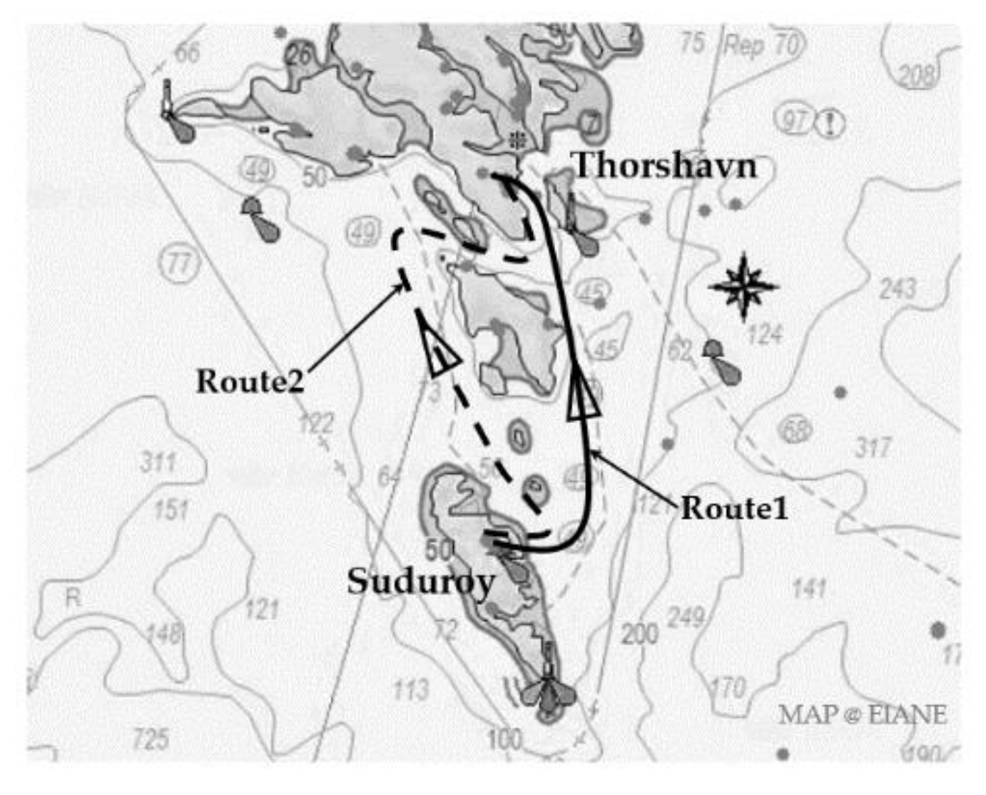
The data used in this article was provided by the Danish University of Technology and comes from a passenger roll-on roll-off (ro-ro) ship operating from the port of Thorshavn, capital of the Faroe Islands to Suduroy [5]. A single voyage takes approximately two hours, with two to three round trips per day. Its main routes are shown via the Elane route data in Figure 6. Route 1 (R1) is the main route, and Route 2 (R2) is the backup route when R1 is experiencing heavy weather and sea conditions. The experimental data contained fifty-two voyages, including 40 voyages using the R1 route and 12 voyages using the R2 route. The main particulars of the case ship are listed in

Table 1. Principal particulars of the case ship.

Parameters	Value
LOA (Length Overall)	135 m
Molded Width	22.7 m
Molded Depth	8.1 m
Designed Draft	5.6 m
Designed Speed	21 knots
Main Engine Power	3360 kW (Four)
Auxiliary Engine Power	515 kW (Four)
IMO Number	9275218

.

4.2. Multisource Data Analysis

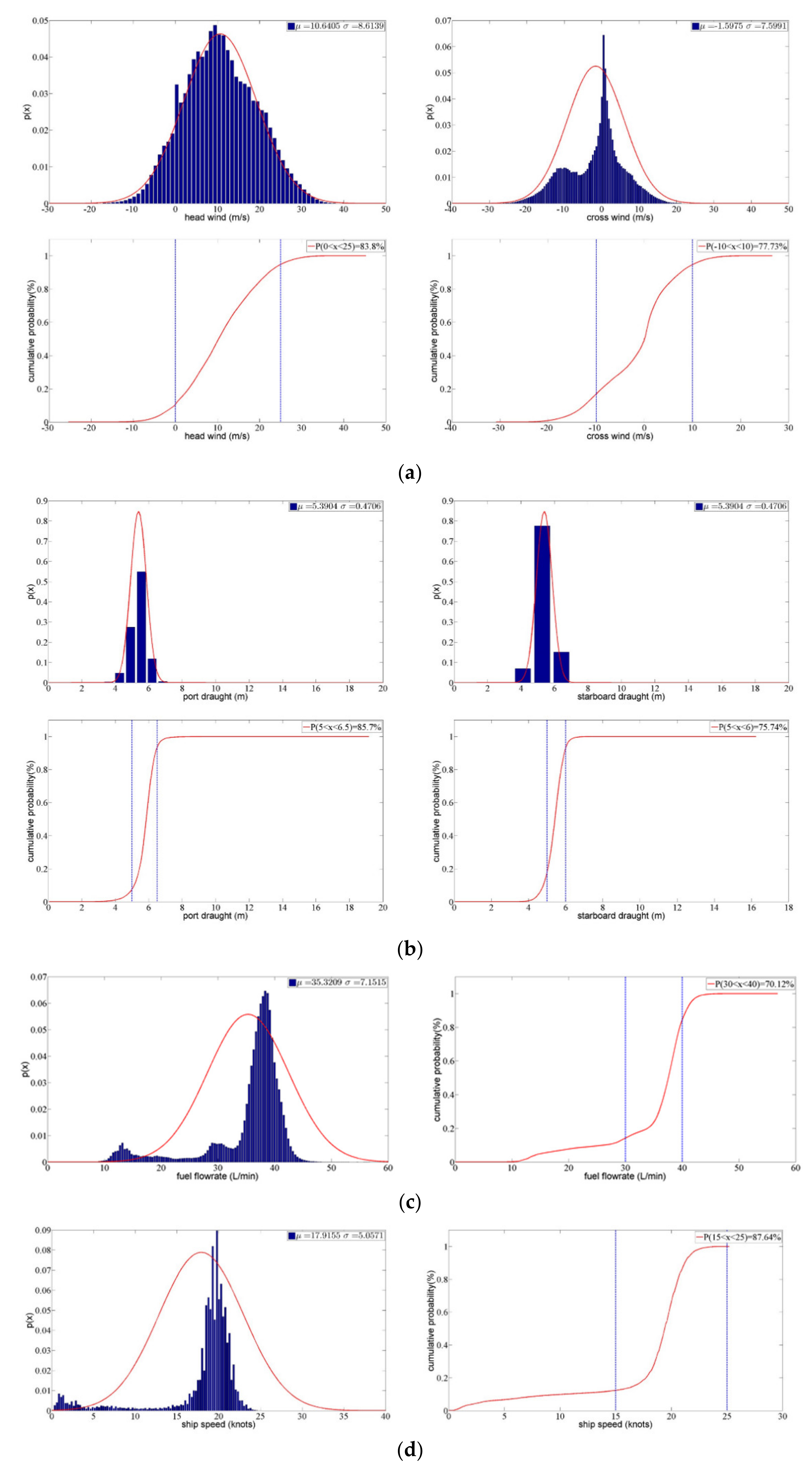
The experimental data were collected by the nine sensors installed aboard ship, namely speed (V) by the Doppler log stern, headwind (H) and crosswind (C) by a wind sensor on the mast, port and starboard rudder angle (Rpor, Rsta) by a rudder angle indicator astern, port and starboard propeller pitch (Ppor, Psta) by a propeller sensor astern, fuel consumption (Fuel) by a fuel flow meter astern, port and starboard draught (Dpor, Dsta) by a radar level meter amidships, trim (T) by pitching adjustors stem and stern. The sampling periods are shown in

Table 2. Sampling period of diverse sensors.

Sensor	Sampling Period (s)
Speed through water	3.00
Trim	0.50
Draught	0.45
Wind speed and direction	2.00
Rudder angle	1.00
Fuel consumption	1.00
Propeller pitch	1.00

. Statistical analysis was carried out for these sensor-based data, as shown in Figure 7. The notation μ and σ in Figure 7 are the mean value and variance of the normal distribution.

The headwind satisfied the normal distribution almost exactly. In total, 83.8% of the data were distributed between 0 to 25 m/s. For crosswind, the distribution was not normally distributed and had two peaks, at −10 m/s and 0 m/s. A total of 77.73% of the data were between −10 and 10 m/s, showing that the crosswind from the port and starboard sides was nearly equal (see Figure 7a).

The draught also satisfied the normal distribution. The draught had little change, from 5 to 6 m. This reflected that the ship was a passenger ship and did not need to load cargo, so loading conditions did not change significantly. The draught of the port and starboard were nearly equal, indicating that the ship did not list (see Figure 7b).

4.3. Heterogeneous Data Feature Fusion

4.3.1. Optimization of Frame Size and Overlap Size

As previously mentioned, the moving-overlapped frame can better maintain the continuity of the data in comparison with the nonoverlapped frame. To verify this, an indicator termed the mean interval error (MIE) was defined as the mean value of the data interval error.

The formula for calculating MIE was shown as follows:

$$\mathrm{MIE}=\frac{1}{m-1}{\displaystyle \sum }_{i=1}^{m-1}\left(x_{i+1}-x_i\right)$$

(25)

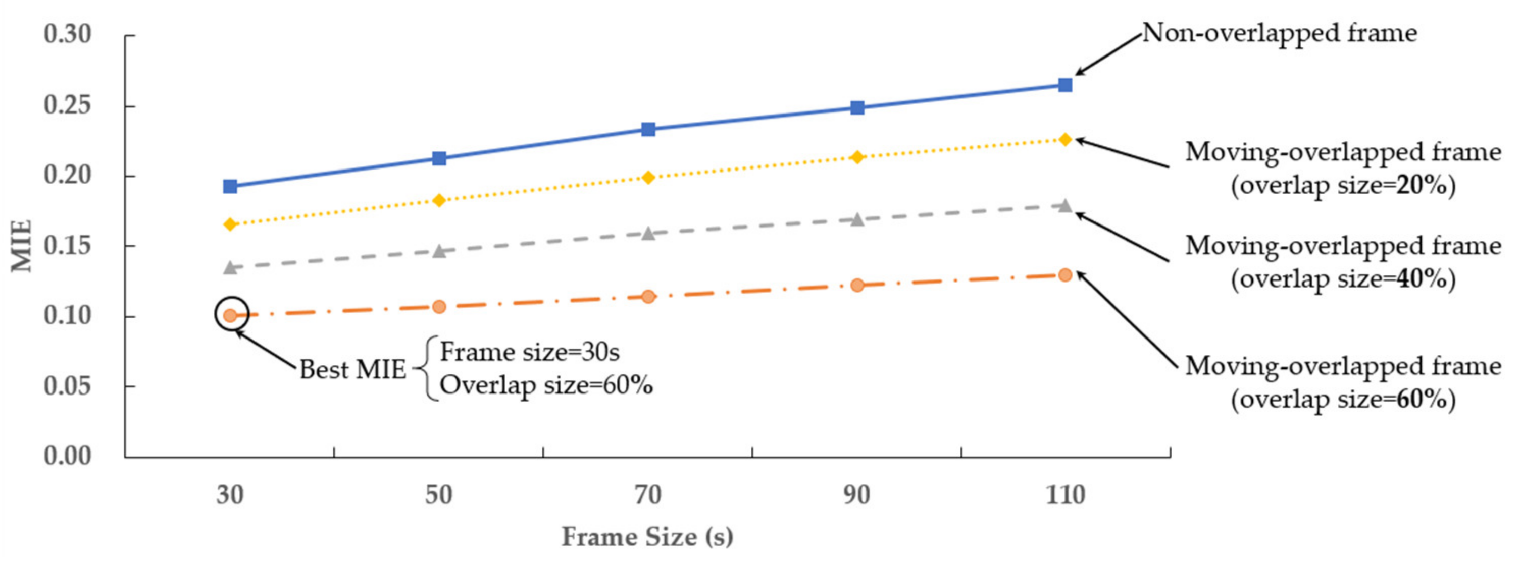
In this section, the influence of frame size and overlap size on MIE is discussed. This paper compares two different framing methods, namely nonoverlapped frames and moving overlapped frames. The data processing’s pseudo code is shown in Algorithm 2. The frame size was set to 30, 50, 70, 90 and 110 s and the overlap size was set as 20, 40 and 60% of the frame size, respectively. The results of the MIE are shown in

Table 3. Mean interval error (MIE) for different framing methods.

Frame Size (s)	MIE
	Nonoverlapped Frame	Moving Overlapped Frame
		Overlap Size (20%)	Overlap Size (40%)	Overlap Size (60%)
30	0.19	0.17	0.13	0.10
50	0.21	0.18	0.15	0.11
70	0.23	0.20	0.16	0.11
90	0.25	0.21	0.17	0.12
110	0.26	0.23	0.18	0.13

and Figure 8.

Algorithm 2 Data processing algorithm of framing

Input: d (frame size), l (overlap size), D (original sensor data), C (framing methods)

1: N, number of windows

Output: SF. A, SF. B, TSF

2: Initialize: SF. A←Ø, SF. B←Ø, TSF←Ø

3: Framing, find the start point Ts and end point Te of original sensor data sequence D

4: if C=Nonoverlapped frame then

5:  N=(Te−Ts)/d

6:  for i=1 to N do

7:   Si =D(Ts +(i−1)*d, Ts +(i*d))

8:  end for

9: end if

10: if C=Moving-overlapped frame then

11:  N= (Te -d-Ts)/((1-l) *d)

12:  for i= 1 to N do

13:   Si = D(Ts +(i−1)*(1-l)*d, Ts +(i−1)*(1-l)*d+d)

14:  end for

15: end if

16: for each Si do

17:  SF. A. append ([mean(Si), variance(Si), mean difference(Si), median(Si), mode(Si)])

18:  SF. B. append ([Max(Si), Q3(Si), median(Si), Q2(Si), Min(Si)])

19:  TSF. append (extract_TSF(Si))

20: end for

As can be seen from Figure 8, when the frame size changed from 30 to 110, the MIE of the moving overlapped frame was always lower than that of the nonoverlapped frame. With the increments of frame size, the MIE of both the moving-overlapped frame and nonoverlapped frame increased. For the overlap size, the larger the overlap size, the smaller the MIE. It can be seen that the moving overlapped framing method better maintained the continuity characteristics of the original sensor data.

4.3.2. Optimization of TSF Clusters

In this section, the cluster number of the TSF is discussed. An indicator called area error (AE) is given in Equation (26). The AE is the deviation between the area under the original data curve and the extracted TSF feature. The smaller the AE, the better the extracted TSF feature preserves the original data information.

$$\mathrm{AE}=\left|S_{feature}-S_{original}\right|$$

(26)

Experimentally, the cluster number was set to 2, 3, 4 and 5. The results are shown in

Table 4. Area error (AE) of different cluster numbers.

Cluster Numbers	k = 2	k = 3	k = 4	k = 5
AE	246.02	199.56	148.20	123.04

. The experimental results showed that with the increase in cluster number, the AE decreased, which means that the larger the cluster number, the better the TSF maintained the information of the original data.

4.3.3. Setting of Feature Fusion

In this section, the AE of features after fusion is discussed. From Section 4.3.2, it is concluded that the AE can indicate the ability of features to preserve original data information. The ability of the fused features such as (SF. A, TSF), (SF. B, TSF) and (SF. A, SF. B, TSF) were evaluated, and the results are shown in

Table 5. AE of fused features.

Features	TSF	(SF. A, TSF)	(SF. B, TSF)	(SF. A, SF. B, TSF)
AE	123.04	108.36	72.09	79.22

.

The results show that the AE was decreased when statistics features were fused with TSF. The (SF. A, TSF) fusion decreased the AE by 11.9%, while the (SF. A, SF. B, TSF) fusion decreased the AE by 35.6%. The best performance was obtained by (SF. B, TSF) with a decrease of 41.4% in the AE. In general, with fused features, the AE is decreased and data information was better preserved.

4.4. SFC Model Establishment and Estimation

4.4.1. Evaluation Indicator

The root mean squared error (RMSE) is the square root of the mean square deviation of the estimated SFC from the real SFC for a number of observations m. A smaller value of RMSE means that the estimation results obtained by the integrated SFC estimation model better approximated the real value. The calculation formula of the RMSE is shown in Equation (27), where ${\widehat{y}}_{i+1}=f\left(x\right)$ is the estimated value and $y_{i+1}$. is the real value.

$$\mathrm{RMSE}=\sqrt{\frac{1}{m-1}{\displaystyle \sum }_{i=1}^{m-1}{\left({\widehat{y}}_{i+1}-y_{i+1}\right)}^2}$$

(27)

4.4.2. Comparison of SFC Models

In order to investigate the application of different feature extraction methods on various machine learning methods, three machine learning methods were adopted to train SFC models, namely LR, SVR and ANN. Different feature extraction methods were compared, namely SF. A, SF. B and TSF. Moreover, statistical features were combined with TSF, giving combinations (SF. A, TSF), (SF. B, TSF) and (SF. A, SF. B, TSF). The SF. A and SF. B were also combined. The parameters of the machine learning methods are discussed below.

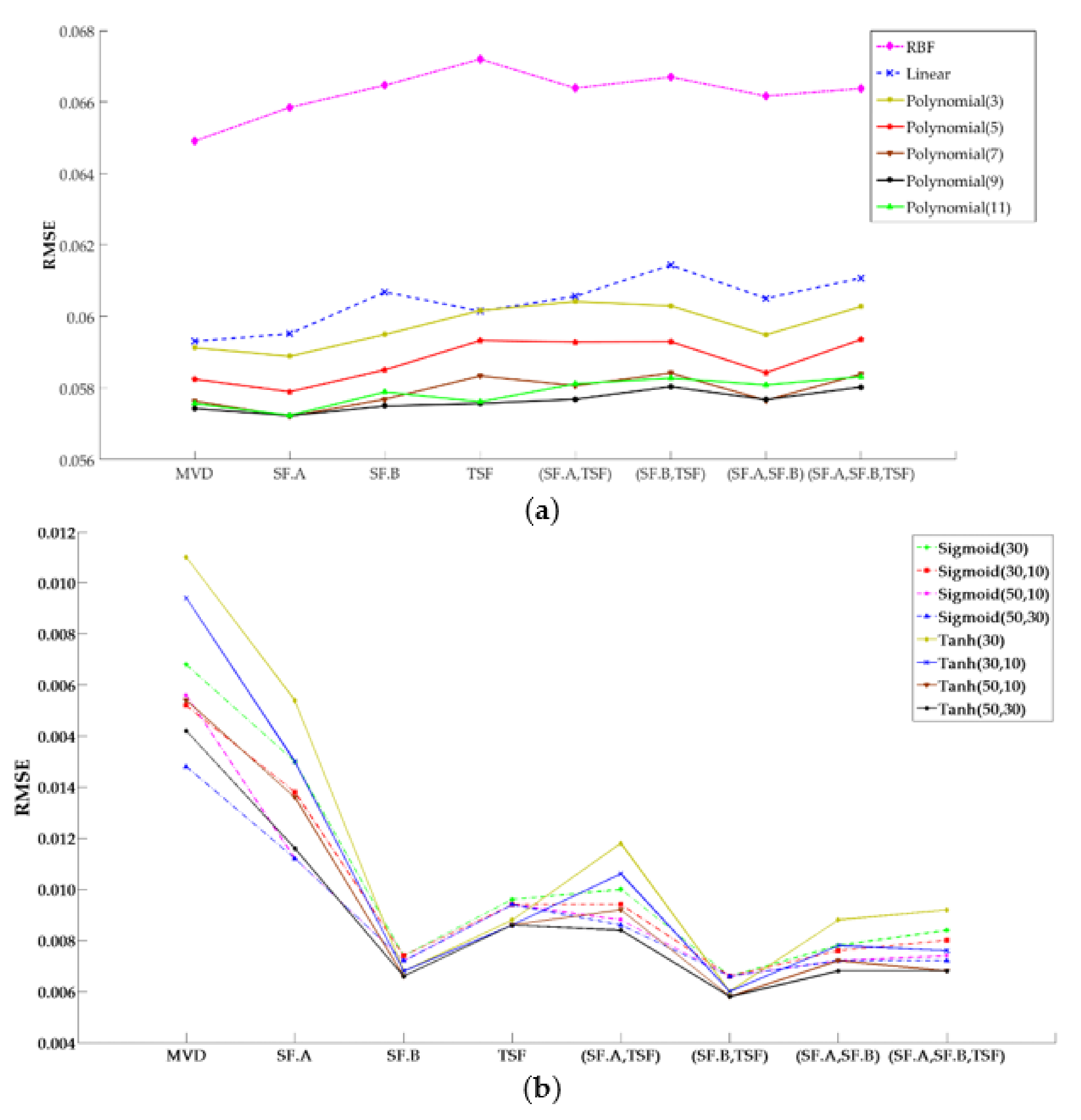
The penalty factor in SVR had little effect on the estimation accuracy and was set as 1.0 in the experiments. Three kernel functions were adopted, namely radial basis function (RBF), linear and polynomial. For the polynomial kernel function, the polynomial degree varied between 3 and 11. The results are illustrated in Figure 9a, which shows that the polynomial kernel function of degree 9 obtained the best estimation accuracy. In the ANN, two types of activation functions were adopted, namely Tanh and Sigmoid. The best estimation results were obtained by the Tanh activation function with two hidden layers, the first of 50 neurons, and the second of 30 neurons, as shown in Figure 9b. With the optimized parameters, the proposed feature extraction methods were compared with the method adopted in [5]. The results are shown in

Table 6. Comparison of feature extraction methods based on various machine learning methods.

Feature Extraction Methods	LR	SVR (Polynomial)	ANN (Two Hidden Layers (50,30))
MVD	0.0105	0.0574	0.0101
SF. A	0.0104	0.0572	0.0078
SF. B	0.0103	0.0575	0.0053
TSF	0.0119	0.0576	0.0063
(SF. A, TSF)	0.0102	0.0577	0.0062
(SF. B, TSF)	0.0099	0.0577	0.0049
(SF. A, SF. B)	0.0098	0.0580	0.0054
(SF. A, SF. B, TSF)	0.0096	0.0580	0.0054

and Figure 10.

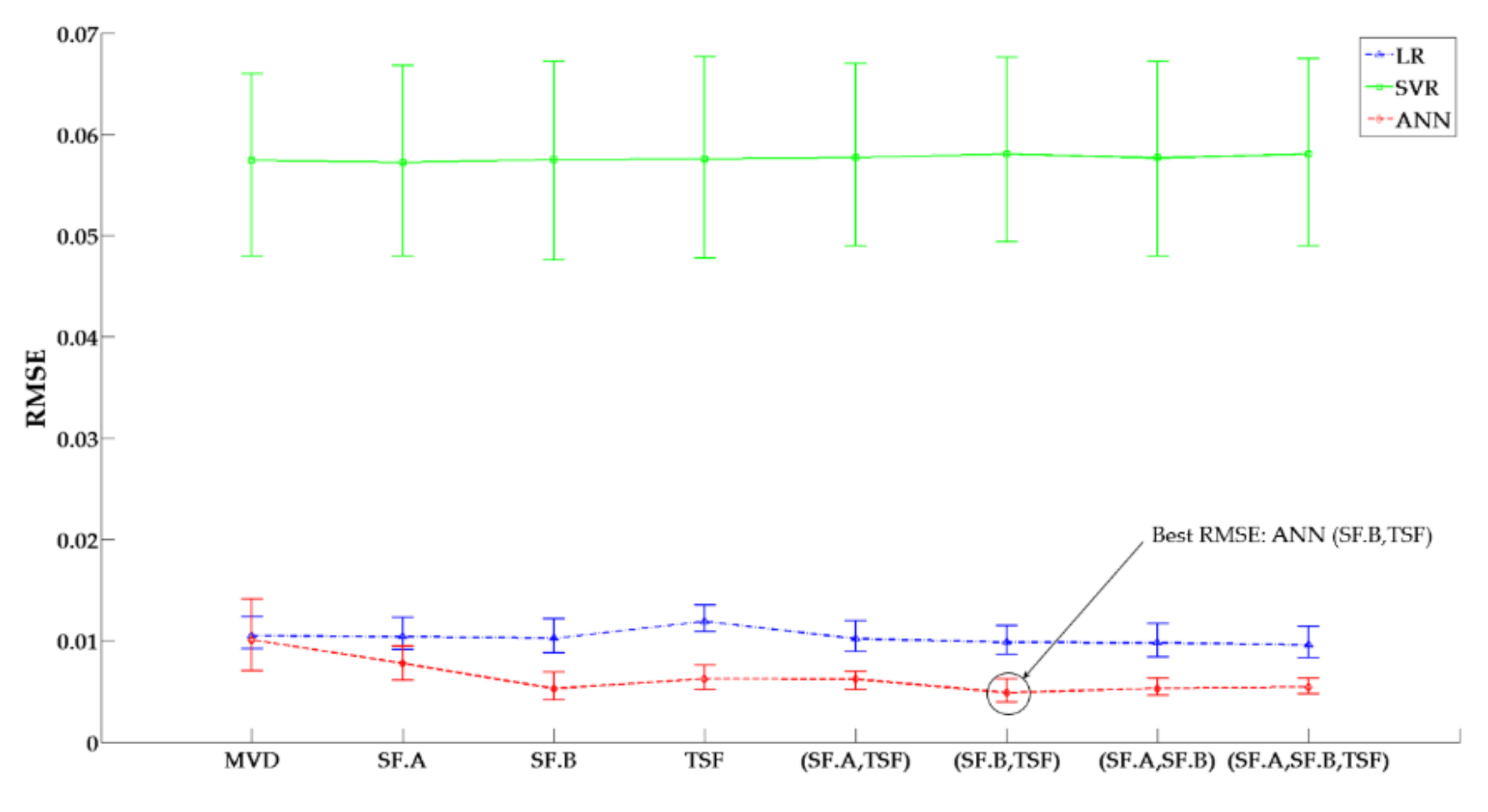
As can be seen from Table 6 and Figure 10, the accuracy of ANN was the best, followed by LR and SVR (polynomial). For LR, the SF. A could improve the RMSE with 0.9%, while SF. B improved the RMSE by 1.9%. When time sequence characteristics were considered, the RMSE improved by 2.8% and 5.7% with (SF. A, TSF), and (SF. B, TSF), respectively. The best result was shown for (SF. A, SF. B, TSF), with an improvement of 8.5%. The overall accuracy of the SVR model was not very good. Only the SF. A improved the RMSE by 0.35%. In general, ANN had a better performance with higher accuracy. With SF. A, SF. B and TSF, the RMSE was improved by 22.8, 47.5 and 37.6%, respectively. Combining TSF with statistical features, (SF. A, TSF) and (SF. B, TSF) improved the RMSE by 38.6 and 51.5%. The (SF. A, SF. B) and (SF. A, SF. B, TSF) showed little improvement compared with SF.B. The accuracy of (SF. A, SF. B) was even lower than SF.B.

In summary, with the proposed model, the estimation accuracy could be improved for some frequently adopted machine learning methods. The best estimation result was obtained using (SF. B, TSF) with ANN. For LR, better performance was achieved by (SF. A, SF. B, TSF). The SF. A was more useful for SVR (polynomial).

4.5. Fuel Consumption Estimation of Real Voyages

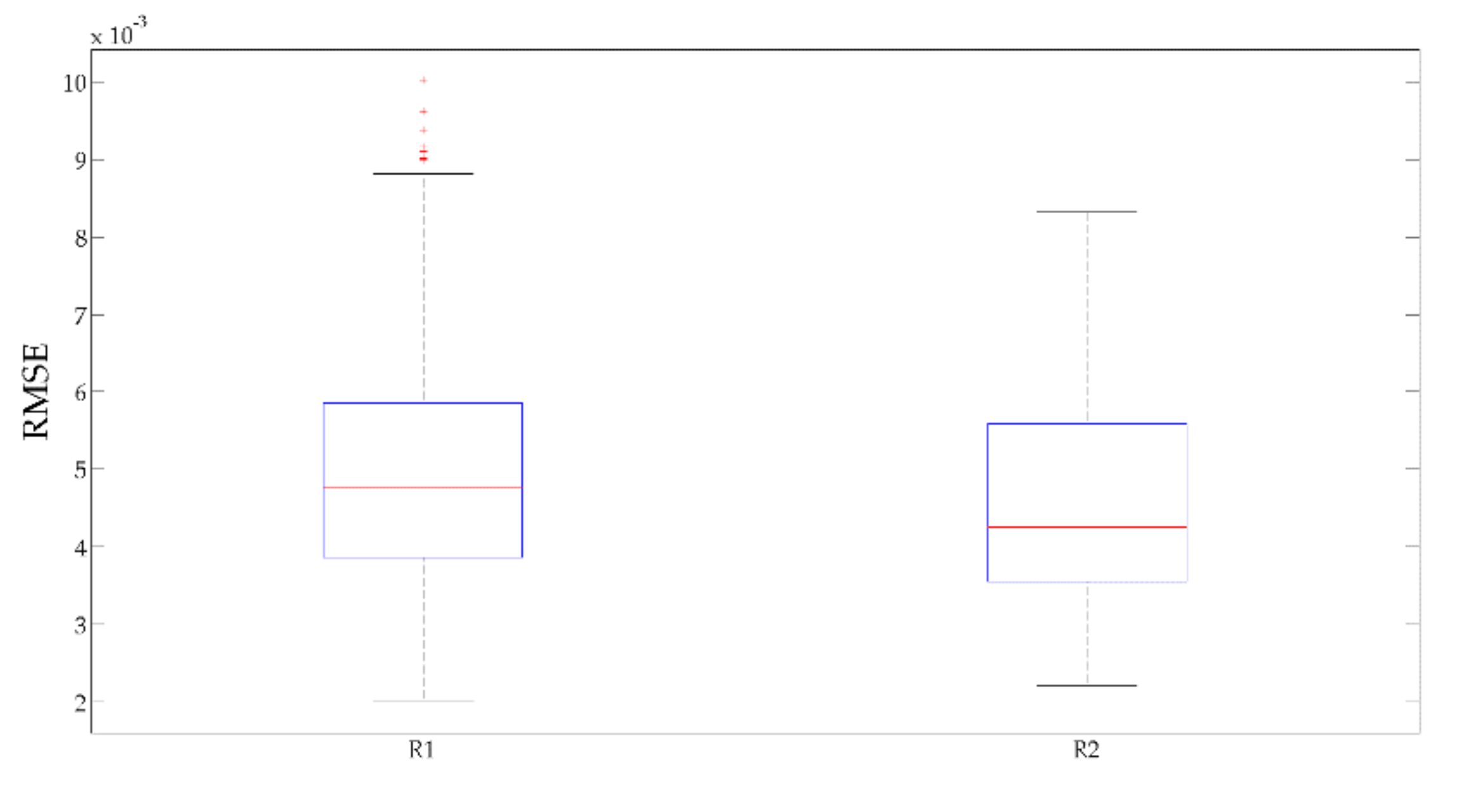
After finishing the model establishment procedure, the SFC of a real ship on voyages could be estimated. As mentioned in Section 4.1, there were two routes for the case ship, forty voyages for R1 and 12 voyages for R2. From the machine learning method and feature comparison of Section 4.4, the ANN combined with (SF. B, TSF) features were adopted.

For both R1 and R2, a boxplot of the estimation error was given, and the results are shown in Figure 11. The RMSE of R1 and R2 were extremely close to each other, varying from 0.002 to 0.009. For both R1 and R2, the model performed well in providing an estimation result. This proved that the model can perform a favorably for different routes.

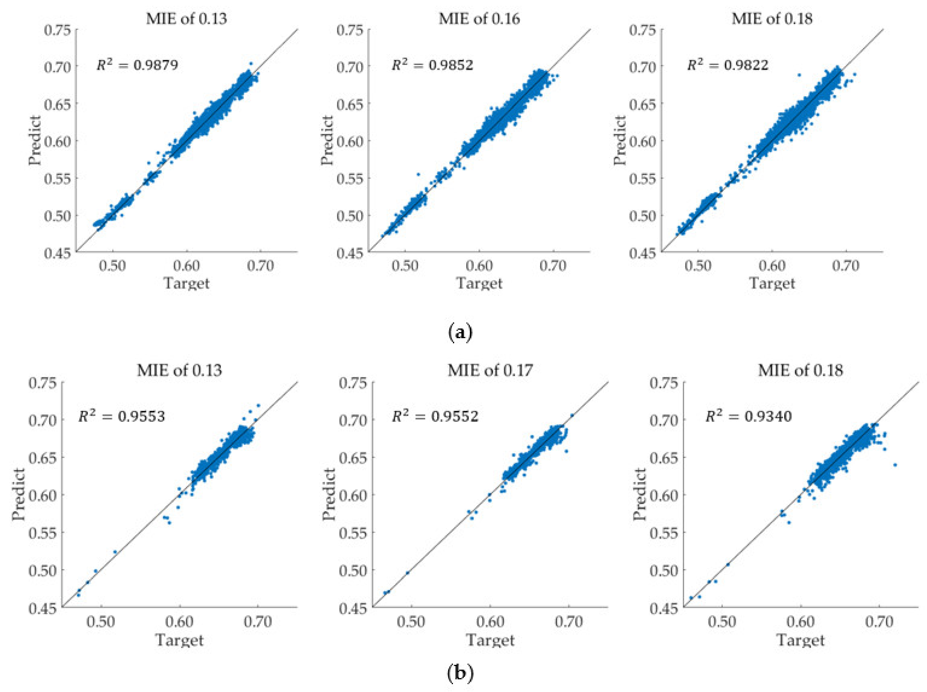
The estimation accuracy of different MIE was also discussed and the R-squared of different with different MIE for both routes is shown in Figure 12. For the R2, the fuel consumption mainly distributed between 0.60 to 0.70. The R1 also mainly distributed between 0.60 to 0.70, but still had a big part within 0.50 to 0.60. The experimental results showed that with the increasement of MIE, the R-squared of both routes decreased. The larger MIE made it difficult to estimate the fuel consumption rate exactly.

5. Conclusions

This study proposed an integrated SFC model consisting of three parts: a multisource data collection module, a heterogeneous data feature fusion module and a fuel consumption estimation module. In the multisource data collection module, data types and collection methods were introduced. In heterogeneous data feature fusion module, to fuse the heterogeneous data, feature extraction and fusion were adopted. In the fuel consumption estimation module, three machine learning methods were used to train the integrated SFC model.

The academic contributions of this paper can be summarized as follows. (a) For unifying the time domain of multisource data, the framing method was adopted. Two framing methods were compared, and it was found that the moving overlapped frame was more effective. (b) The TSF feature was proposed to consider the time sequence characteristics of data. Statistical features and TSF were fused for considering both data distribution and time sequence. (c) The fused (SF. B, TSF) feature had a better estimation accuracy with ANN, especially for the R1.

For further studies, we will continue to improve the framing methods and feature fusion methods to obtain a smaller MIE and better prediction accuracy of fuel consumption estimation. We will also examine the application of the proposed model on other real-world cases of SFC analysis and prediction.

References

- United Nations Conference on Trade and Development. Review of Maritime Transport; United Nations: New York, NY, USA, 2019. [Google Scholar]
- Beşikçi, E.B.; Arslan, O.; Turan, O.; Ölçer, A.I. An artificial neural network-based decision support system for energy effi-cient ship operations. Comput. Oper. Res. 2016, 66, 393–401. [Google Scholar] [CrossRef] [Green Version]
- Stopford, M. Maritime Economics; Routledge: London, UK, 2013. [Google Scholar]
- Zheng, J.; Zhang, H.; Yin, L.; Liang, Y.; Wang, B.; Li, Z.; Song, X.; Zhang, Y. A voyage with minimal fuel consumption for cruise ships. J. Clean. Prod. 2019, 215, 144–153. [Google Scholar] [CrossRef]
- Petersen, J.P. Mining of Ship Operation Data for Energy Conservation. Ph.D Thesis, Technical University of Denmark, Lyngby, Denmark, 2011. [Google Scholar]
- Petersen, J.P.; Winther, O.; Jacobsen, D.J. A Machine-Learning Approach to Predict Main Energy Consumption under Realistic Operational Conditions. Ship Technol. Res. 2012, 59, 64–72. [Google Scholar] [CrossRef]
- Rui, Y.E.; Xu, J. Vessel fuel consumption model based on neural network. Ship Eng. 2016, 38, 85–88. [Google Scholar]
- Yin, Z.; Xu, J. Ship oil consumption optimization based on sailing data. Ship Eng. 2019, 41, 100–104. [Google Scholar]
- Le Luan Thanh, P.K.-S.; Gunwoo, L.; Hwayoung, K. Neural network-based fuel consumption estimation for container ships in Korea. Marit. Policy. Manag. 2020, 47, 615–632. [Google Scholar]
- Yasser, B.; Farag, A.; Ler, A.I. The development of a ship performance model in varying operating conditions based on ANN and regression techniques. Ocean Eng. 2020, 198, 106972. [Google Scholar]
- Moreira, L.; Vettor, R.; Soares, C.G. Neural Network Approach for Predicting Ship Speed and Fuel Consumption. J. Mar. Sci. Eng. 2021, 9, 119. [Google Scholar] [CrossRef]
- Leifsson, L.T.; Sven, H.; Sigursson, S.P.; Ari, V. Grey-box modeling of an ocean vessel for operational optimization. Simul. Model. Pract. Theory 2008, 16, 923–932. [Google Scholar] [CrossRef]
- Panapakidis, I.; Sourtzi, V.-M.; Dagoumas, A. Forecasting the Fuel Consumption of Passenger Ships with a Combination of Shallow and Deep Learning. Electronics 2020, 9, 776. [Google Scholar] [CrossRef]
- Mou, X.; Yuan, Y.; Yan, X.; Zhao, G. A prediction model of fuel consumption for inland river ships based on random forest regression. J. Transp. Inf. Saf. 2017, 35, 100–105. [Google Scholar]
- Yan, S.; Wang, R.; Du, Y. Development of a two-stage ship fuel consumption prediction and reduction model for a dry bulk ship. Transp. Res. Pt. E Logist. Transp. Rev. 2020, 138, 101930. [Google Scholar] [CrossRef]
- Gkerekos, C.; Lazakis, I.; Theotokatos, G. Machine learning models for predicting ship main engine Fuel Oil Consumption: A comparative study. Ocean Eng. 2019, 188, 106282. [Google Scholar] [CrossRef]
- Peng, Y.; Liu, H.; Li, X.; Huang, J.; Wang, W. Machine learning method for energy consumption prediction of ships in port considering green ports. J. Clean. Prod. 2020, 264, 121564. [Google Scholar] [CrossRef]
- Meng, Q.; Du, Y.; Wang, Y. Shipping log data based container ship fuel efficiency modeling. Transp. Res. Part B Methodol. 2016, 83, 207–229. [Google Scholar] [CrossRef]
- Vujović, I.; Šoda, J.; Kuzmanić, I.; Petković, M. Predicting External Influences to Ship’s Average Fuel Consumption Based on Non-Uniform Time Set. J. Mar. Sci. Eng. 2020, 8, 625. [Google Scholar] [CrossRef]
- Wang, S.; Ji, B.; Zhao, J.; Liu, W.; Xu, T. Predicting ship fuel consumption based on LASSO regression. Transp. Res. Part D Transp. Environ. 2018, 65, 817–824. [Google Scholar] [CrossRef]
- Tayfun, U.; Karatuğ, Ç.; Yasin, A. Machine learning approach to ship fuel consumption: A case of container vessel. Transp. Res. Part D Transp. Environ. 2020, 84, 102389. [Google Scholar]
- Soner, O.; Akyuz, E.; Celik, M. Statistical modelling of ship operational performance monitoring problem. J. Mar. Sci. Technol. 2018, 24, 543–552. [Google Scholar] [CrossRef]
- Bocchetti, D.; Lepore, A.; Palumbo, B.; Vitiello, L. A statistical approach to ship fuel consumption monitoring. J. Ship Res 2015, 59, 162–171. [Google Scholar] [CrossRef]
- Bialystocki, N.; Konovessis, D. On the estimation of ship’s fuel consumption and speed curve: A statistical approach. Ocean Eng. Sci. 2016, 1, 157–166. [Google Scholar] [CrossRef] [Green Version]
- Lu, R.; Turan, O.; Boulougouris, E.; Banks, C.; Incecik, A. A semi-empirical ship operational performance prediction model. Ocean Eng. 2015, 110, 18–28. [Google Scholar] [CrossRef] [Green Version]
- Yang, L.; Chen, G.; Rytter, N.G.M.; Jinlou, Z.; Dong, Y. A genetic algorithm-based grey-box model for ship fuel consumption prediction towards sustainable shipping. Ann. Oper. Res. 2019. [Google Scholar] [CrossRef]
- Perera, L.P.; Mo, B. Data analysis on marine engine operating regions in relation to ship navigation. Ocean Eng. 2016, 128, 163–172. [Google Scholar] [CrossRef]
- Trodden, D.; Murphy, A.J.; Pazouki, K.; Sargeant, J. Fuel usage data analysis for efficient shipping operations. Ocean Eng. 2015, 110, 75–84. [Google Scholar] [CrossRef] [Green Version]
- Perera, L.P.; Mo, B. Ship performance and navigation data compression and communication under autoencoder system architecture. J. Ocean Eng. Sci. 2018, 3, 133–143. [Google Scholar] [CrossRef]
- Zhou, S.; Xie, S.; Pan, C. Probability Theory and Mathematical Statistics, 4rd ed.; Zhejiang University Press: Hangzhou, China, 2008. [Google Scholar]
Figure 1.
Overview of fuel consumption estimation process.
Figure 2.
Sensor-based ship fuel consumption (SFC) data and multisource data: (a) multiple sensors aboard ships; (b) multisource data fusion.
Figure 3.
Two different framing methods: (a) nonoverlapped frame; (b) moving overlapped frame.
Figure 4.
Statistics feature extraction: (a) MVD; (b) SF. A; (c) SF. B.
Figure 5.
Extraction of TSF from sensor frame.
Figure 6.
Main route of the case ship.
Figure 7.
Statistical analysis of variables: (a) headwind and crosswind; (b) port and starboard draught; (c) fuel flowrate; (d) ship speed.
Figure 8.
MIE of different framing methods.
Figure 9.
Parameter tuning results: (a) support vector regression (SVR); (b) artificial neural network (ANN).