
The Use of Animal-Borne Biologging and Telemetry Data to Quantify Spatial Overlap of Wildlife with Marine Renewables

 , ,
, ,
Abstract
:1. Introduction
2. Materials and Methods
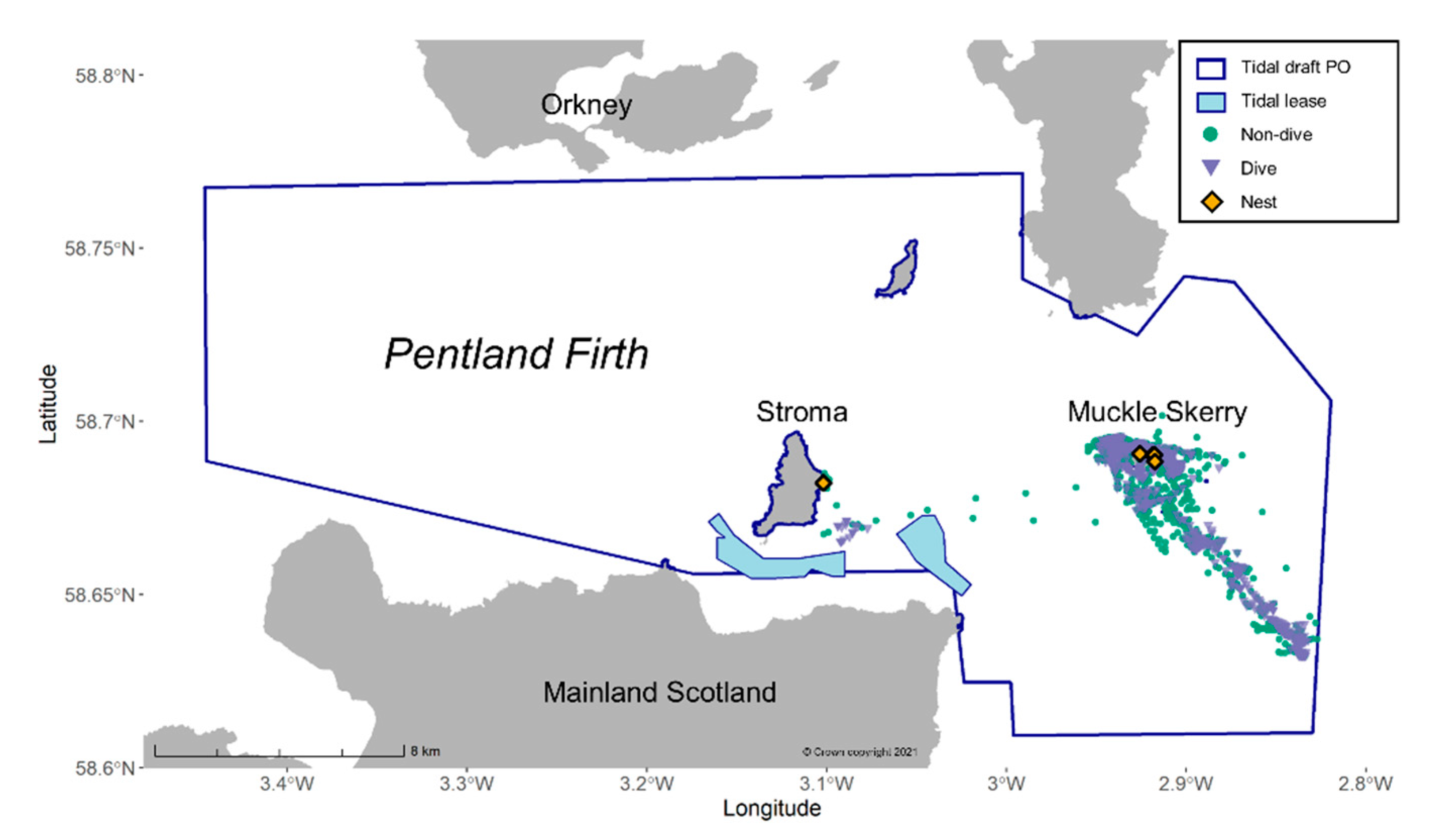
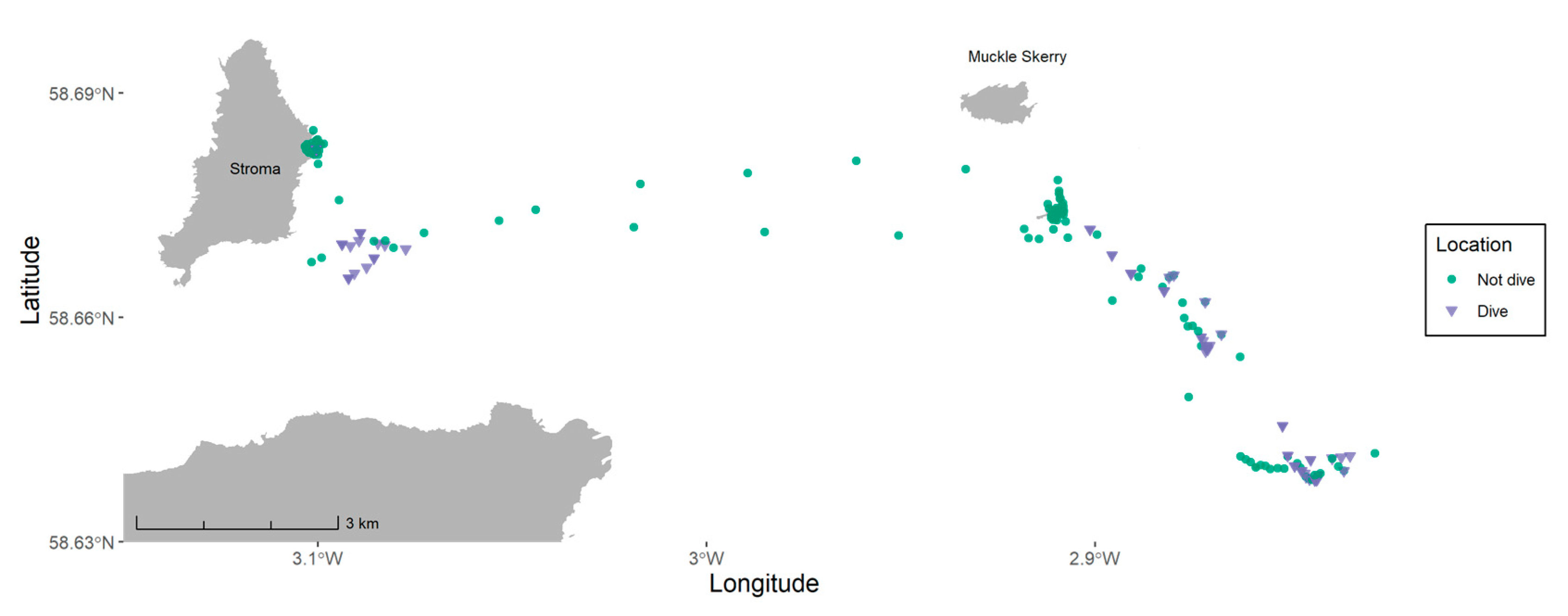
2.1. Study Site
2.2. Bird-Borne Biologging and Telemetry Dataset
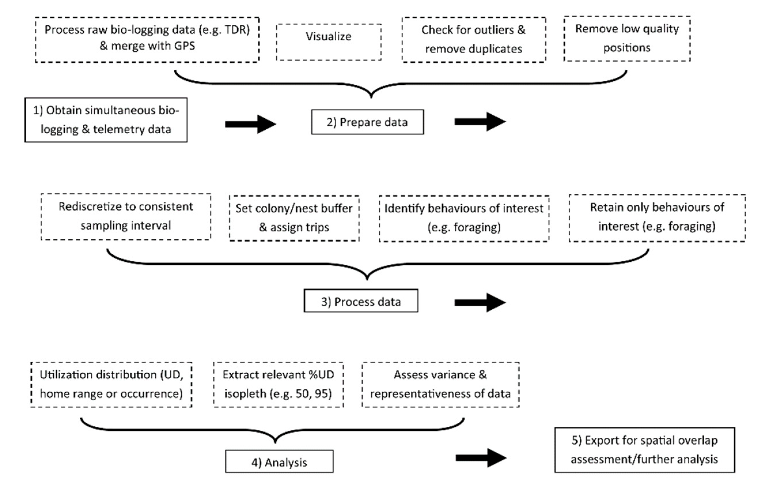
2.3. Workflow Description
2.3.1. Preparation and Processing
2.3.2. Utilization Distributions
2.3.3. Variance and Representativeness
2.4. Overlap with Tidal Development and Lease Sites
3. Results
4. Discussion
Supplementary Materials
Author Contributions
Funding
Institutional Review Board Statement
Informed Consent Statement
Data Availability Statement
Acknowledgments
Conflicts of Interest
Appendix A. Worked Example of Data Preparation, Processing and Analysis for One Shag
Appendix A.1. Step 2: Data Preparation
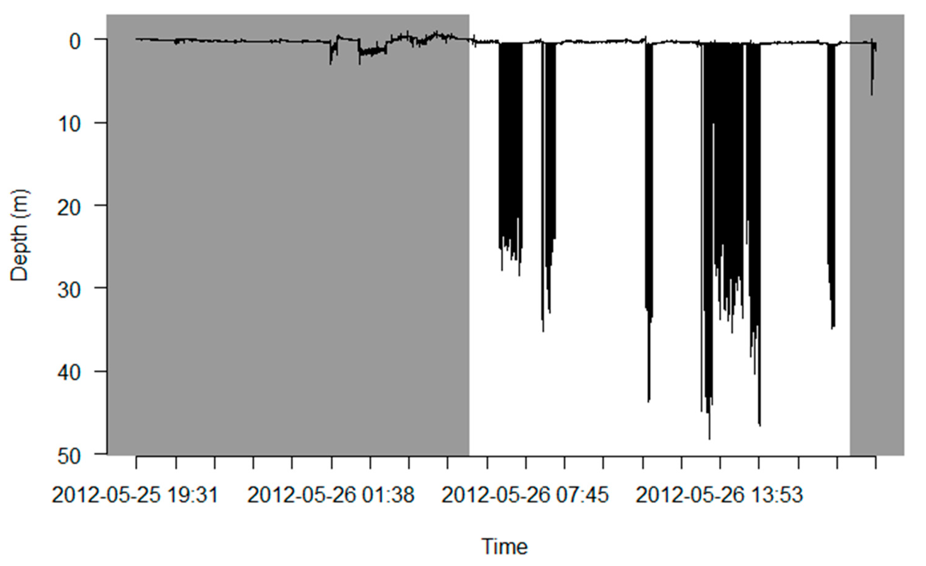
Appendix A.1.1. Process Raw Biologging Data (e.g., TDR) and Merge with GPS
Read in TDR and GPS Data

Create TDR Object


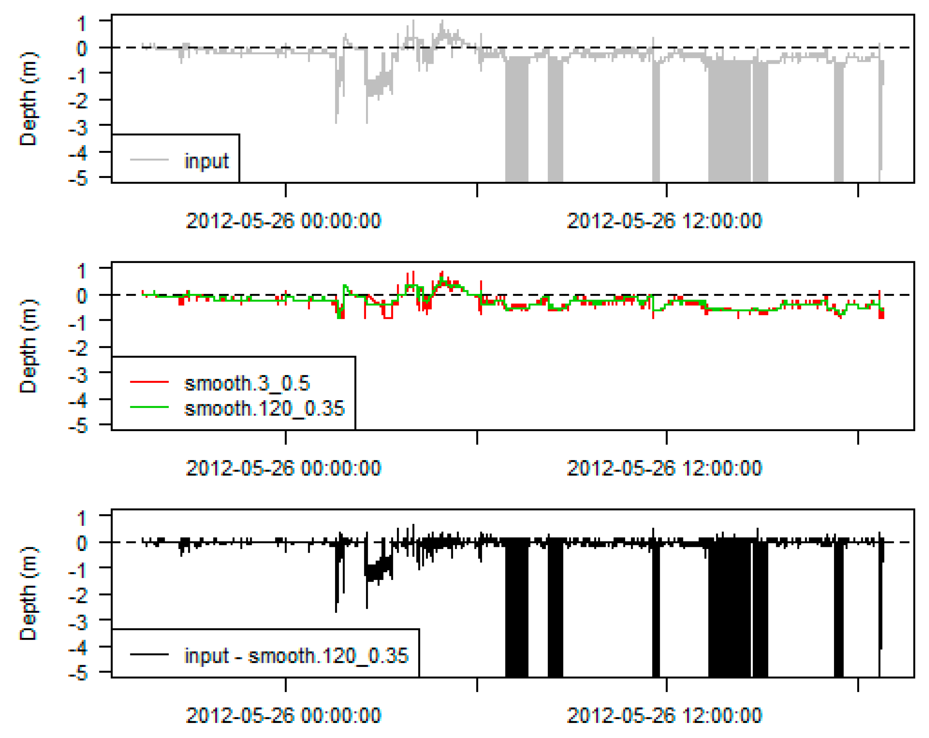
Choose Smoothing Parameters


Calibrate Data

Extract Data


Merge TDR with Simultaneous GPS Data


Tidy

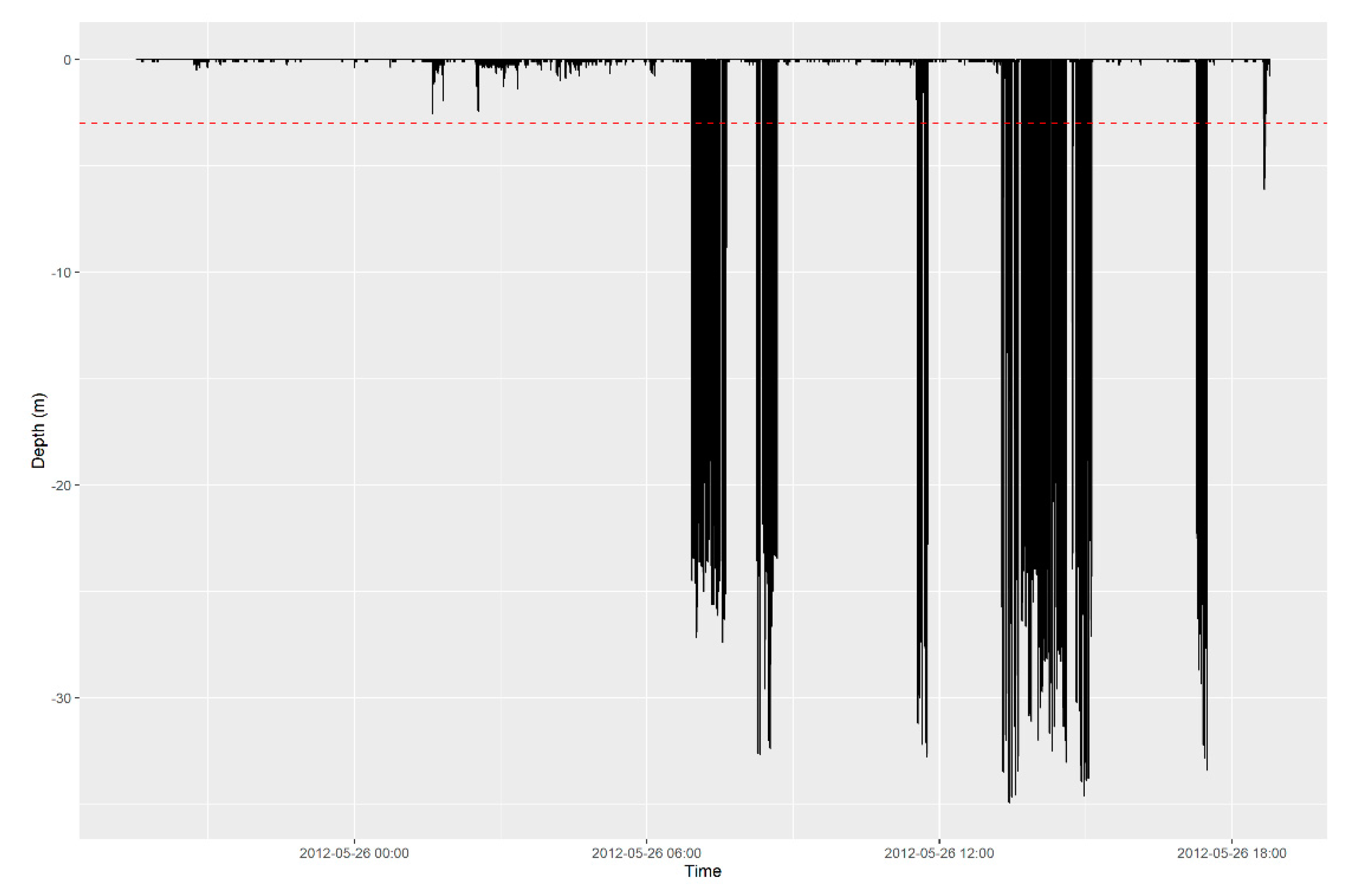
Appendix A.1.2. Visualize

Appendix A.1.3. Check for Outliers and Remove Duplicates

Appendix A.1.4. Remove Low Quality Positions
Appendix A.2. Step 3: Data Processing
Appendix A.2.1. Rediscretize to Consistent Sampling Interval


Appendix A.2.2. Set Colony/Nest Buffer and Assign Trips


Appendix A.2.3. Identify Behaviors of Interest
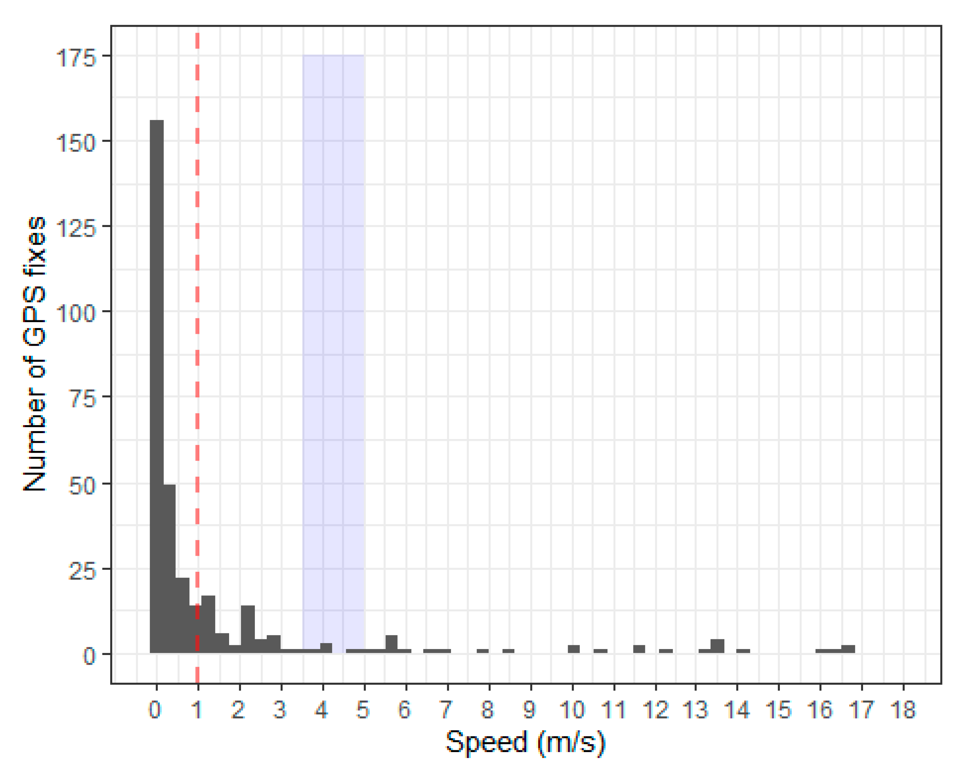
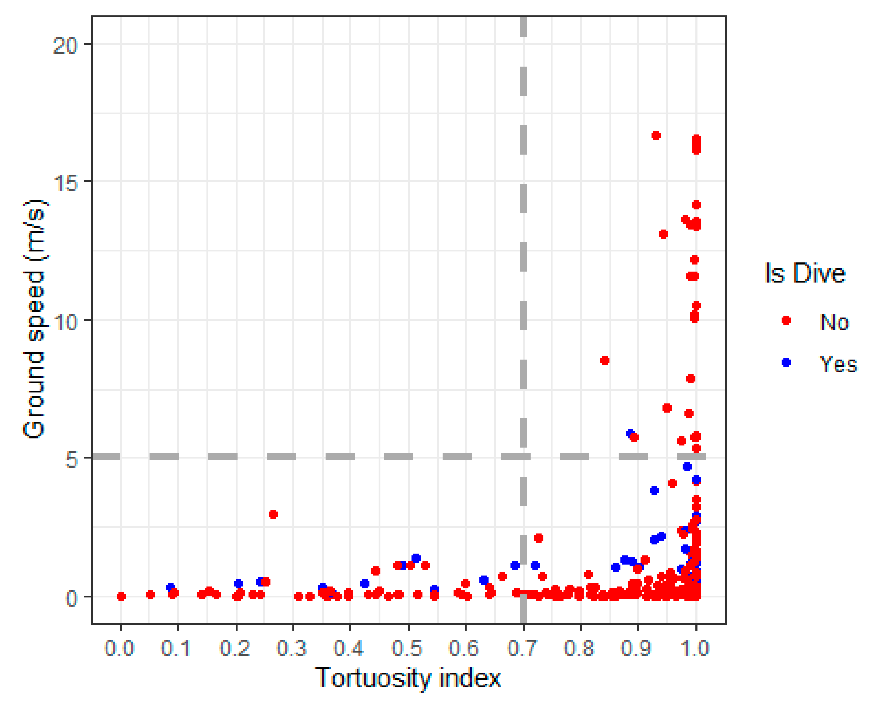
Appendix A.3. Speed

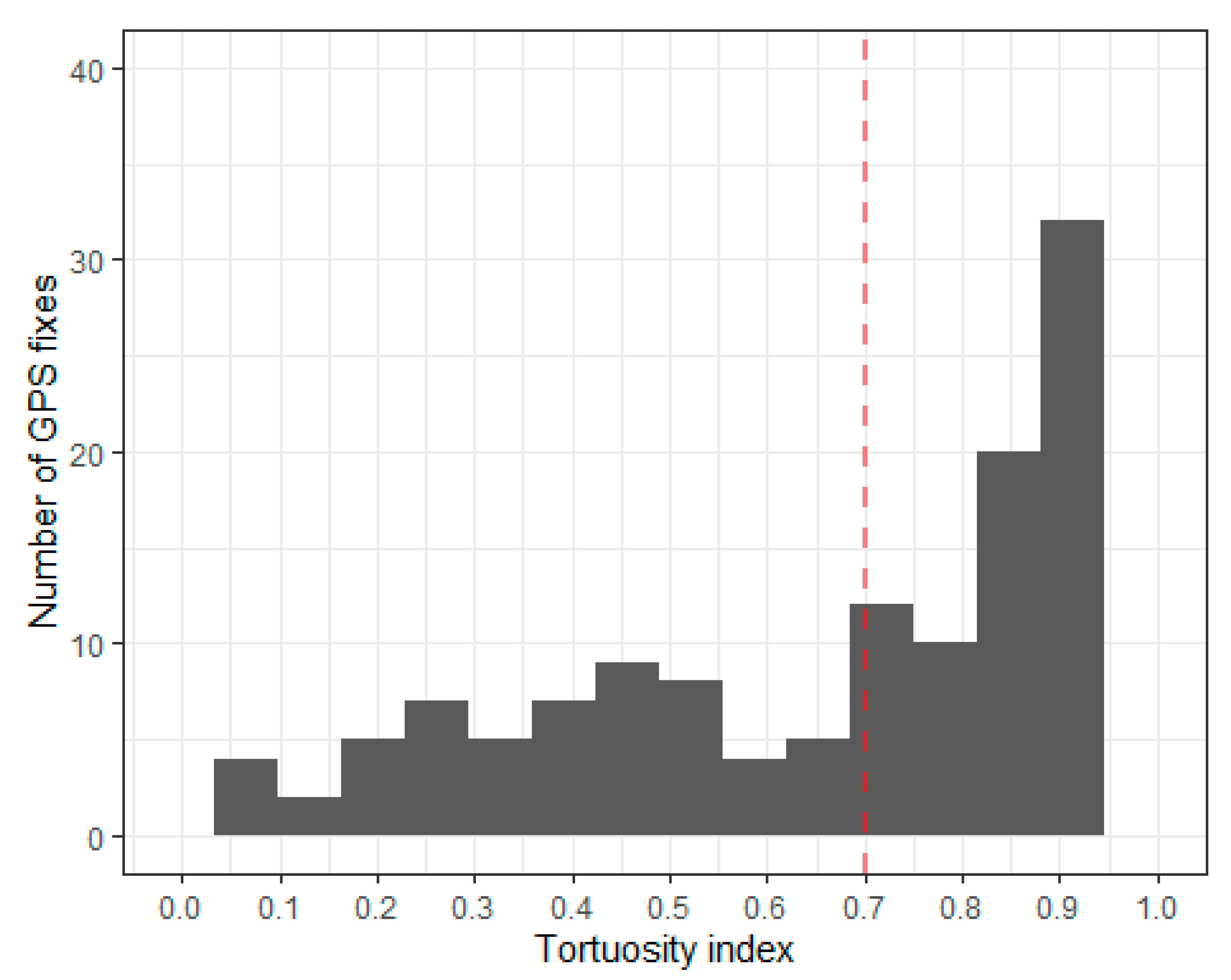
Appendix A.4. Tortuosity


Appendix A.5. Identify Flight Using Speed, Tortuosity and Dive Classification

Retain Only Behaviors of Interest


Appendix A.6. Step 4: Analysis
Appendix A.6.1. Utilization Distribution


Appendix A.6.2. Extract Relevant % UD Isopleth


Appendix B

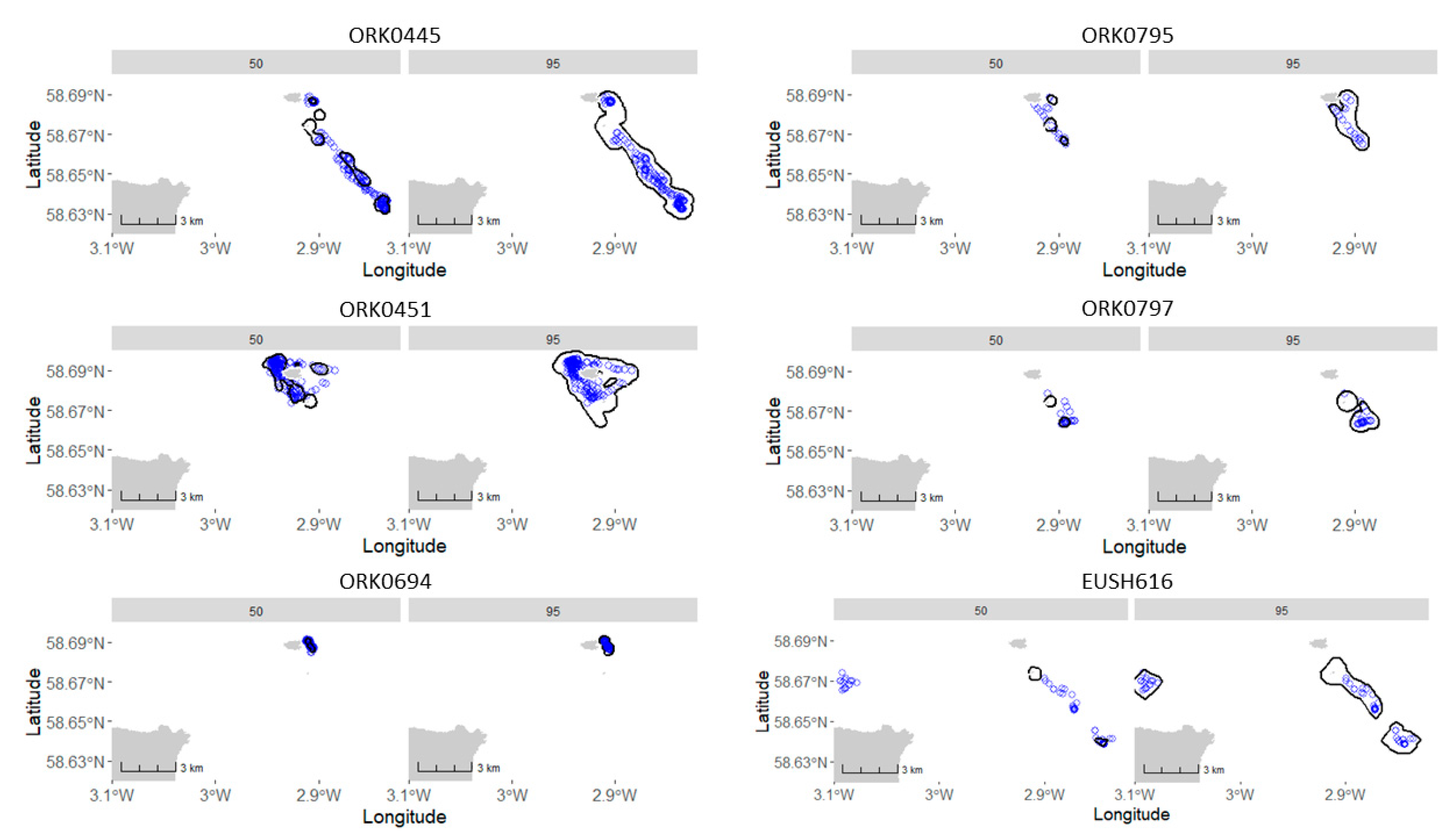
| ID | UD Level | Ratio (%) |
|---|---|---|
| EUSH_616 | 50 | 18 |
| EUSH_616 | 95 | 100 |
| EUSH_ORK0445 | 50 | 65.9 |
| EUSH_ORK0445 | 95 | 100 |
| EUSH_ORK0451 | 50 | 86.1 |
| EUSH_ORK0451 | 95 | 100 |
| EUSH_ORK0694 | 50 | 99.2 |
| EUSH_ORK0694 | 95 | 100 |
| EUSH_ORK0795 | 50 | 41.2 |
| EUSH_ORK0795 | 95 | 100 |
| EUSH_ORK0797 | 50 | 52.6 |
| EUSH_ORK0797 | 95 | 94.7 |

Appendix C


References
- Intergovernmental Panel on Climate Change. Climate Change 2014: Mitigation of Climate Change; Cambridge University Press: Cambridge, UK, 2014. [Google Scholar]
- The European Parliament and the Council of the European Union Directive 2009/ 28/EC of the European parliament and of the council of 23 April on the promotion of the use of energy from renewable sources and amending and subsequently repealing Directives 2001/77/EC and 2003/30/EC. Off. J. Eur. Union I. 2009, 140, 16–62.
- Copping, A.E.; Freeman, M.C.; Gorton, A.M.; Hemery, L.G. Risk Retirement—Decreasing Uncertainty and Informing Consenting Processes for Marine Renewable Energy Development. J. Mar. Sci. Eng. 2020, 8, 172. [Google Scholar] [CrossRef] [Green Version]
- Green, D.R. Geospatial Technologies for Siting Coastal and Marine Renewable Infrastructures. Geoinform. Mar. Coast. Manag. 2016, 269–296. [Google Scholar]
- Copping, A.E.; Hemery, L.G.; Overhus, D.M.; Garavelli, L.; Freeman, M.C.; Whiting, J.M.; Gorton, A.M.; Farr, H.K.; Rose, D.J.; Tugade, L.G. Potential Environmental Effects of Marine Renewable Energy Development—The State of the Science. J. Mar. Sci. Eng. 2020, 8, 879. [Google Scholar] [CrossRef]
- Benjamins, S.; Dale, A.; Hastie, G.; Waggitt, J.; Lea, M.-A.; Scott, B.; Wilson, B. Confusion Reigns? A Review of Marine Megafauna Interactions with Tidal-Stream Environments. Oceanogr. Mar. Biol. 2015, 1–54. [Google Scholar] [CrossRef]
- Wilson, B.; Batty, R.S.; Daunt, F.; Carter, C. Collision Risks between Marine Renewable Energy Devices and Mammals, Fish and Diving Birds; Report to the Scottish Executive; Scottish Association for Marine Science: Oban, UK, 2007; 110p. [Google Scholar]
- Furness, R.W.; Wade, H.M.; Robbins, A.M.C.; Masden, E.A. Assessing the sensitivity of seabird populations to adverse effects from tidal stream turbines and wave energy devices. ICES J. Mar. Sci. 2012, 69, 1466–1479. [Google Scholar] [CrossRef] [Green Version]
- Fraser, S.; Williamson, B.J.; Nikora, V.; Scott, B.E. Fish distributions in a tidal channel indicate the behavioural impact of a marine renewable energy installation. Energy Rep. 2018, 4, 65–69. [Google Scholar] [CrossRef]
- Joy, R.; Wood, J.D.; Sparling, C.E.; Tollit, D.J.; Copping, A.E.; McConnell, B.J. Empirical measures of harbor seal behavior and avoidance of an operational tidal turbine. Mar. Pollut. Bull. 2018, 136, 92–106. [Google Scholar] [CrossRef]
- Johnston, D.W.; Read, A.J. Flow-field observations of a tidally driven island wake used by marine mammals in the Bay of Fundy, Canada. Fish. Oceanogr. 2007, 16, 422–435. [Google Scholar] [CrossRef]
- Isaksson, N.; Masden, E.A.; Williamson, B.J.; Costagliola-Ray, M.M.; Slingsby, J.; Houghton, J.D.R.; Wilson, J. Assessing the effects of tidal stream marine renewable energy on seabirds: A conceptual framework. Mar. Pollut. Bull. 2020, 157, 111314. [Google Scholar] [CrossRef]
- Waggitt, J.J.; Scott, B.E. Using a spatial overlap approach to estimate the risk of collisions between deep diving seabirds and tidal stream turbines: A review of potential methods and approaches. Mar. Policy 2014, 44, 90–97. [Google Scholar] [CrossRef] [Green Version]
- Marine Scotland. Planning Scotland’s Seas: Sectoral Marine Plans for Offshore Wind, Wave and Tidal Energy in Scottish Waters; Scottish Government: Edinburgh, UK, 2013; pp. 1–85.
- Scottish Government. Sectoral Marine Plan for Offshore Wind Energy; Scottish Government: Edinburgh, UK, 2020.
- Cooke, S.J.; Hinch, S.G.; Wikelski, M.; Andrews, R.D.; Kuchel, L.J.; Wolcott, T.G.; Butler, P.J. Biotelemetry: A mechanistic approach to ecology. Trends Ecol. Evol. 2004, 19, 334–343. [Google Scholar] [CrossRef]
- Burger, A.E.; Shaffer, S.A. Application of tracking and data-logging technology in research and conservation of seabirds. Auk 2008, 125, 253–264. [Google Scholar] [CrossRef] [Green Version]
- Hussey, N.E.; Kessel, S.T.; Aarestrup, K.; Cooke, S.J.; Cowley, P.D.; Fisk, A.T.; Harcourt, R.G.; Holland, K.N.; Iverson, S.J.; Kocik, J.F.; et al. Aquatic animal telemetry: A panoramic window into the underwater world. Science 2015, 348, 1255642. [Google Scholar] [CrossRef] [Green Version]
- Kays, R.; Crofoot, M.C.; Jetz, W.; Wikelski, M. Terrestrial animal tracking as an eye on life and planet. Science 2015, 348, aaa2478. [Google Scholar] [CrossRef] [Green Version]
- Dujon, A.M.; Lindstrom, R.T.; Hays, G.C. The accuracy of Fastloc-GPS locations and implications for animal tracking. Methods Ecol. Evol. 2014, 5, 1162–1169. [Google Scholar] [CrossRef]
- Halsey, L.G.; Bost, C.A.; Handrich, Y. A thorough and quantified method for classifying seabird diving behaviour. Polar Biol. 2007, 30, 991–1004. [Google Scholar] [CrossRef]
- Schreer, J.F.; Testa, J.W. Statistical Classification of Diving Behavior. Mar. Mammal Sci. 1995, 11, 85–93. [Google Scholar] [CrossRef]
- Hays, G.C.; Ferreira, L.C.; Sequeira, A.M.M.; Meekan, M.G.; Duarte, C.M.; Bailey, H.; Bailleul, F.; Bowen, W.D.; Caley, M.J.; Costa, D.P.; et al. Key Questions in Marine Megafauna Movement Ecology. Trends Ecol. Evol. 2016, 31, 463–475. [Google Scholar] [CrossRef] [Green Version]
- McGowan, J.; Beger, M.; Lewison, R.L.; Harcourt, R.; Campbell, H.; Priest, M.; Dwyer, R.G.; Lin, H.Y.; Lentini, P.; Dudgeon, C.; et al. Integrating research using animal-borne telemetry with the needs of conservation management. J. Appl. Ecol. 2017, 54, 423–429. [Google Scholar] [CrossRef]
- Hays, G.C.; Koldewey, H.J.; Andrzejaczek, S.; Attrill, M.J.; Barley, S. A review of a decade of lessons from one of the world’s largest MPAs: Conservation gains and key challenges. Mar. Biol. 2020, 167, 1–22. [Google Scholar] [CrossRef]
- Queiroz, N.; Humphries, N.E.; Couto, A.; Vedor, M.; da Costa, I.; Sequeira, A.M.M.; Mucientes, G.; Santos, A.M.; Abascal, F.J.; Abercrombie, D.L.; et al. Global spatial risk assessment of sharks under the footprint of fisheries. Nature 2019, 572, 461–466. [Google Scholar] [CrossRef] [Green Version]
- Handley, J.M.; Pearmain, E.J.; Oppel, S.; Carneiro, A.P.B.; Hazin, C.; Phillips, R.A.; Ratcliffe, N.; Staniland, I.J.; Clay, T.A.; Hall, J.; et al. Evaluating the effectiveness of a large multi-use MPA in protecting Key Biodiversity Areas for marine predators. Divers. Distrib. 2020, 1–15. [Google Scholar] [CrossRef] [Green Version]
- Bedriñana-Romano, L.; Hucke-Gaete, R.; Viddi, F.A.; Johnson, D.; Zerbini, A.N.; Morales, J.; Mate, B.; Palacios, D.M. Defining priority areas for blue whale conservation and investigating overlap with vessel traffic in Chilean Patagonia, using a fast-fitting movement model. Sci. Rep. 2021, 11, 1–16. [Google Scholar] [CrossRef] [PubMed]
- Thaxter, C.B.; Ross-Smith, V.H.; Bouten, W.; Masden, E.A.; Clark, N.A.; Conway, G.J.; Barber, L.; Clewley, G.D.; Burton, N.H.K. Dodging the blades: New insights into three-dimensional space use of offshore wind farms by lesser black-backed gulls Larus fuscus. Mar. Ecol. Prog. Ser. 2018, 587, 247–253. [Google Scholar] [CrossRef]
- Russell, D.J.F.; Brasseur, S.M.J.M.; Thompson, D.; Hastie, G.D.; Janik, V.M.; Aarts, G.; McClintock, B.T.; Matthiopoulos, J.; Moss, S.E.W.; McConnell, B. Marine mammals trace anthropogenic structures at sea. Curr. Biol. 2014, 24, 638–639. [Google Scholar] [CrossRef] [Green Version]
- Hastie, G.D.; Gillespie, D.M.; Gordon, J.C.D.; Macaulay, J.D.J.; McConnell, B.J.; Sparling, C.E. Tracking Technologies for Quantifying Marine Mammal Interactions with Tidal Turbines: Pitfalls and Possibilities. In Marine Renewable Energy Technology and Environmental Interactions; Springer: Dordrecht, The Netherlands, 2014; pp. 127–139. [Google Scholar]
- Wood, A.G.; Prince, P.A.; Croxall, J.P.; Quantifying, J.P. Quantifying habitat use in satellite-tracked pelagic seabirds: Application of kernel estimation to albatross locations. J. Avian Biol. 2000, 31, 278–286. [Google Scholar] [CrossRef]
- Bandeira De Melo, L.F.; Lima Sábato, M.A.; Vaz Magni, E.M.; Young, R.J.; Coelho, C.M. Secret lives of maned wolves (Chrysocyon brachyurus Illiger 1815): As revealed by GPS tracking collars. J. Zool. 2007, 271, 27–36. [Google Scholar] [CrossRef]
- Shillinger, G.L.; Palacios, D.M.; Bailey, H.; Bograd, S.J.; Swithenbank, A.M.; Gaspar, P.; Wallace, B.P.; Spotila, J.R.; Paladino, F.V.; Piedra, R.; et al. Persistent leatherback turtle migrations present opportunities for conservation. PLoS Biol. 2008, 6, 1408–1416. [Google Scholar] [CrossRef] [Green Version]
- Vander Wal, E.; Rodgers, A.R. An individual-based quantitative approach for delineating core areas of animal space use. Ecol. Modell. 2012, 224, 48–53. [Google Scholar] [CrossRef]
- Reisinger, R.R.; Raymond, B.; Hindell, M.A.; Bester, M.N.; Crawford, R.J.M.; Davies, D.; de Bruyn, P.J.N.; Dilley, B.J.; Kirkman, S.P.; Makhado, A.B.; et al. Habitat modelling of tracking data from multiple marine predators identifies important areas in the Southern Indian Ocean. Divers. Distrib. 2018, 24, 535–550. [Google Scholar] [CrossRef] [Green Version]
- Lascelles, B.G.; Taylor, P.R.; Miller, M.G.R.; Dias, M.P.; Oppel, S.; Torres, L.; Hedd, A.; Le Corre, M.; Phillips, R.A.; Shaffer, S.A.; et al. Applying global criteria to tracking data to define important areas for marine conservation. Divers. Distrib. 2016, 22, 422–431. [Google Scholar] [CrossRef] [Green Version]
- Cleasby, I.R.; Wakefield, E.D.; Bearhop, S.; Bodey, T.W.; Votier, S.C.; Hamer, K.C. Three-dimensional tracking of a wide-ranging marine predator: Flight heights and vulnerability to offshore wind farms. J. Appl. Ecol. 2015, 52, 1474–1482. [Google Scholar] [CrossRef] [Green Version]
- Stewart, B.; Leatherwood, S.; Yochem, P.K. Harbor Seal Tracking and Telemetry by Satellite. Mar. Mammal Sci. 1989, 5, 361–375. [Google Scholar] [CrossRef]
- Vandenabeele, S.; Wilson, R.; Grogan, A. Tags on seabirds: How seriously are instrument-induced behaviours considered? Anim. Welf. 2011, 20, 559–571. [Google Scholar]
- Cagnacci, F.; Boitani, L.; Powell, R.A.; Boyce, M.S. Animal ecology meets GPS-based radiotelemetry: A perfect storm of opportunities and challenges. Philos. Trans. R. Soc. B Biol. Sci. 2010, 365, 2157–2162. [Google Scholar] [CrossRef] [PubMed] [Green Version]
- Lewis, K.P.; Vander Wal, E.; Fifield, D.A. Wildlife biology, big data, and reproducible research. Wildl. Soc. Bull. 2018, 42, 172–179. [Google Scholar] [CrossRef]
- Wade, H.M.; Masden, E.A.; Jackson, A.C.; Furness, R.W. Incorporating data uncertainty when estimating potential vulnerability of Scottish seabirds to marine renewable energy developments. Mar. Policy 2016, 70, 108–113. [Google Scholar] [CrossRef]
- Easton, M.C.; Woolf, D.K.; Bowyer, P.A. The dynamics of an energetic tidal channel, the Pentland Firth, Scotland. Cont. Shelf Res. 2012, 48, 50–60. [Google Scholar] [CrossRef]
- Bryden, I.G.; Couch, S.J.; Owen, A.; Melville, G. Tidal current resource assessment. Proc. IMechE 2007, 221, 125–135. [Google Scholar] [CrossRef] [Green Version]
- Marine Scotland. Tidal Energy in Scottish Waters. Initial Plan Framework (Draft Plan Options); Marine Scotland: Aberdeen, UK, 2013; pp. 1–28.
- MeyGen Ltd. MeyGen Tidal Energy Project Phase 1 Environmental Statement. Environ. Impact Assess. 2012, 1–1153. [Google Scholar]
- Browning, E.; Bolton, M.; Owen, E.; Shoji, A.; Guilford, T.; Freeman, R. Predicting animal behaviour using deep learning: GPS data alone accurately predict diving in seabirds. Methods Ecol. Evol. 2018, 9, 681–692. [Google Scholar] [CrossRef] [Green Version]
- Masden, E.A.; Foster, S.; Jackson, A.C. Diving behaviour of Black Guillemots Cepphus grylle in the Pentland Firth, UK: Potential for interactions with tidal stream energy developments. Bird Study 2013, 60, 547–549. [Google Scholar] [CrossRef]
- Shoji, A.; Aris-Brosou, S.; Owen, E.; Bolton, M.; Boyle, D.; Fayet, A.; Dean, B.; Kirk, H.; Freeman, R.; Perrins, C.; et al. Foraging flexibility and search patterns are unlinked during breeding in a free-ranging seabird. Mar. Biol. 2016, 163, 1–10. [Google Scholar] [CrossRef] [PubMed] [Green Version]
- R Core Team. R: A Language and Environment for Statistical Computing; R Core Team: Vienna, Austria, 2019. [Google Scholar]
- Calenge, C. The package “adehabitat” for the R software: A tool for the analysis of space and habitat use by animals. Ecol. Modell. 2006, 197, 516–519. [Google Scholar] [CrossRef]
- Orians, G.H.; Pearson, N.E. On the theory of central place foraging. In Analysis of Ecological Systems; Horn, D.J., Ed.; Ohio State University Press: Columbus, OH, USA, 1979; pp. 155–177. [Google Scholar]
- Christensen-Dalsgaard, S.; Mattisson, J.; Bekkby, T.; Gundersen, H.; May, R.; Rinde, E.; Lorentsen, S.-H. Habitat selection of foraging chick-rearing European shags in contrasting marine environments. Mar. Biol. 2017, 164–196. [Google Scholar] [CrossRef]
- Grémillet, D.; Gallien, F.; El Ksabi, N.; Courbin, N. Sentinels of coastal ecosystems: The spatial ecology of European shags breeding in Normandy. Mar. Biol. 2020, 167, 1–11. [Google Scholar] [CrossRef]
- Votier, S.C.; Bearhop, S.; Witt, M.J.; Inger, R.; Thompson, D.; Newton, J. Individual responses of seabirds to commercial fisheries revealed using GPS tracking, stable isotopes and vessel monitoring systems. J. Appl. Ecol. 2010, 47, 487–497. [Google Scholar] [CrossRef] [Green Version]
- O’Hara Murray, R.; Gallego, A. A modelling study of the tidal stream resource of the Pentland Firth, Scotland. Renew. Energy 2017, 102, 326–340. [Google Scholar] [CrossRef]
- Goddijn-Murphy, L.; Woolf, D.K.; Easton, M.C. Current patterns in the inner sound (Pentland Firth) from underway ADCP data. J. Atmos. Ocean. Technol. 2013, 30, 96–111. [Google Scholar] [CrossRef]
- Bennison, A.; Quinn, J.L.; Debney, A.; Jessopp, M. Tidal drift removes the need for arearestricted search in foraging Atlantic puffins. Biol. Lett. 2019, 15, 20190208. [Google Scholar] [CrossRef] [PubMed] [Green Version]
- Cooper, M.; Bishop, C.; Lewis, M.; Bowers, D.; Bolton, M.; Owen, E.; Dodd, S. What can seabirds tell us about the tide? Ocean Sci. 2018, 14, 1483–1490. [Google Scholar] [CrossRef] [Green Version]
- Shamoun-Baranes, J.; Bouten, W.; Camphuysen, C.J.; Baaij, E. Riding the tide: Intriguing observations of gulls resting at sea during breeding. Ibis 2011, 153, 411–415. [Google Scholar] [CrossRef]
- Worton, B.J. Kernel Methods for Estimating the Utilization Distribution in Home-Range Studies. Ecology 1989, 70, 164–168. [Google Scholar] [CrossRef]
- Kie, J.G.; Matthiopoulos, J.; Fieberg, J.; Powell, R.A.; Cagnacci, F.; Mitchell, M.S.; Gaillard, J.M.; Moorcroft, P.R. The home-range concept: Are traditional estimators still relevant with modern telemetry technology? Philos. Trans. R. Soc. B Biol. Sci. 2010, 365, 2221–2231. [Google Scholar] [CrossRef] [PubMed] [Green Version]
- Ford, R.G.; Krumme, D.W. The analysis of space use patterns. J. Theor. Biol. 1979, 76, 125–155. [Google Scholar] [CrossRef]
- Fleming, C.H.; Fagan, W.F.; Mueller, T.; Olson, K.A.; Leimgruber, P.; Calabrese, J.M. Rigorous home range estimation with movement data: A new autocorrelated kernel density estimator. Ecology 2015, 96, 1182–1188. [Google Scholar] [CrossRef] [Green Version]
- Noonan, M.J.; Tucker, M.A.; Fleming, C.H.; Akre, T.S.; Alberts, S.C.; Ali, A.H.; Altmann, J.; Antunes, P.C.; Belant, J.L.; Beyer, D.; et al. A comprehensive analysis of autocorrelation and bias in home range estimation. Ecol. Monogr. 2019, 89, 1–21. [Google Scholar] [CrossRef]
- Benhamou, S. Dynamic approach to space and habitat use based on biased random bridges. PLoS ONE 2011, 6, e14592. [Google Scholar] [CrossRef] [Green Version]
- Ovaskainen, O. Habitat-specific movement parameters estimated using mark-recapture data and a diffusion model. Ecology 2004, 85, 242–257. [Google Scholar] [CrossRef]
- Horne, J.S.; Garton, E.O.; Krone, S.M.; Lewis, J.S. Analyzing animal movements using Brownian bridges. Ecology 2007, 88, 2354–2363. [Google Scholar] [CrossRef]
- Benhamou, S.; Cornélis, D. Incorporating Movement Behavior and Barriers to Improve Kernel Home Range Space Use Estimates. J. Wildl. Manag. 2010, 74, 1353–1360. [Google Scholar] [CrossRef]
- Pebesma, E. Simple features for R: Standardized Support for Spatial Vector Data. R J. 2018, 10, 439–446. [Google Scholar] [CrossRef] [Green Version]
- Giuggioli, L.; Bartumeus, F. Linking animal movement to site fidelity. J. Math. Biol. 2012, 64, 647–656. [Google Scholar] [CrossRef] [PubMed]
- Augé, A.A.; Chilvers, B.L.; Moore, A.B.; Davis, L.S. Importance of studying foraging site fidelity for spatial conservation measures in a mobile predator. Anim. Conserv. 2014, 17, 61–71. [Google Scholar] [CrossRef]
- Munkres, J. Topology, 2nd ed.; Pearson: Cambridge, UK, 2000. [Google Scholar]
- Lindberg, M.S.; Walker, J. Satellite Telemetry in Avian Research and Management: Sample Size Considerations. J. Wildl. Manag. 2007, 71, 1002–1009. [Google Scholar] [CrossRef]
- Krietsch, J.; Hahn, S.; Kopp, M.; Phillips, R.A.; Peter, H.U.; Lisovski, S. Consistent variation in individual migration strategies of brown skuas. Mar. Ecol. Prog. Ser. 2017, 578, 213–225. [Google Scholar] [CrossRef] [Green Version]
- Sequeira, A.M.M.; Heupel, M.R.; Lea, M.A.; Eguíluz, V.M.; Duarte, C.M.; Meekan, M.G.; Thums, M.; Calich, H.J.; Carmichael, R.H.; Costa, D.P.; et al. The importance of sample size in marine megafauna tagging studies. Ecol. Appl. 2019, 29, e01947. [Google Scholar] [CrossRef]
- Calvo, B.; Furness, R.W. A review of the use and the effects of marks and devices on birds. Ringing Migr. 1992, 13, 129–151. [Google Scholar] [CrossRef] [Green Version]
- Vandenabeele, S.; Shepard, E.; Grémillet, D.; Butler, P.; Martin, G.; Wilson, R. Are bio-telemetric devices a drag? Effects of external tags on the diving behaviour of great cormorants. Mar. Ecol. Prog. Ser. 2015, 519, 239–249. [Google Scholar] [CrossRef]
- Shimada, T.; Thums, M.; Hamann, M.; Limpus, C.J.; Hays, G.C.; FitzSimmons, N.; Wildermann, N.E.; Duarte, C.M.; Meekan, M.G. Optimising sample sizes for animal distribution analysis using tracking data. Methods Ecol. Evol. 2020. [Google Scholar] [CrossRef]
- Soanes, L.M.; Arnould, J.P.Y.; Dodd, S.G.; Sumner, M.D.; Green, J.A. How many seabirds do we need to track to define home-range area? J. Appl. Ecol. 2013, 50, 671–679. [Google Scholar] [CrossRef]
- Thaxter, C.B.; Lascelles, B.; Sugar, K.; Cook, A.S.C.P.; Roos, S.; Bolton, M.; Langston, R.H.W.; Burton, N.H.K. Seabird foraging ranges as a preliminary tool for identifying candidate Marine Protected Areas. Biol. Conserv. 2012, 156, 53–61. [Google Scholar] [CrossRef]
- Scottish Government. Climate Change (Emissions Reduction Targets) (Scotland) Act 2019; Scottish Parliament: Edinburgh, UK, 2019; Volume 5, pp. 1–28.
- Hindell, M.A.; Reisinger, R.R.; Ropert-Coudert, Y.; Hückstädt, L.A.; Trathan, P.N.; Bornemann, H.; Charrassin, J.B.; Chown, S.L.; Costa, D.P.; Danis, B.; et al. Tracking of marine predators to protect Southern Ocean ecosystems. Nature 2020, 580, 87–92. [Google Scholar] [CrossRef] [Green Version]
- Handley, J.; Rouyer, M.; Pearmain, E.J.; Warwick-evans, V.; Teschke, K.; Hinke, J.T.; Lynch, H.; Emmerson, L.; Southwell, C.; Griffith, G.; et al. Marine Important Bird and Biodiversity Areas for Penguins in Antarctica, Targets for Conservation Action. Front. Mar. Sci. 2021, 7. [Google Scholar] [CrossRef]
- Sequeira, A.M.M.; Hays, G.C.; Sims, D.W.; Eguíluz, V.M.; Rodríguez, J.P.; Heupel, M.R.; Harcourt, R.; Calich, H.; Queiroz, N.; Costa, D.P.; et al. Overhauling Ocean Spatial Planning to Improve Marine Megafauna Conservation. Front. Mar. Sci. 2019, 6, 1–12. [Google Scholar] [CrossRef]
- Hays, G.C.; Bailey, H.; Bograd, S.J.; Bowen, W.D.; Campagna, C.; Carmichael, R.H.; Casale, P.; Chiaradia, A.; Costa, D.P.; Cuevas, E.; et al. Translating Marine Animal Tracking Data into Conservation Policy and Management. Trends Ecol. Evol. 2019, 34, 459–473. [Google Scholar] [CrossRef] [Green Version]
- Coyne, M.S.; Godley, B.J. Satellite Tracking and Analysis Tool (STAT): An integrated system for archiving, analyzing and mapping animal tracking data. Mar. Ecol. Prog. Ser. 2005, 301, 1–7. [Google Scholar] [CrossRef] [Green Version]
- Thums, M.; Fernández-Gracia, J.; Sequeira, A.M.M.; Eguíluz, V.M.; Duarte, C.M.; Meekan, M.G. How big data fast tracked human mobility research and the lessons for animal movement ecology. Front. Mar. Sci. 2018, 5, 1–12. [Google Scholar] [CrossRef] [Green Version]
- Williams, H.J.; Taylor, L.A.; Benhamou, S.; Bijleveld, A.I.; Clay, T.A.; de Grissac, S.; Demšar, U.; English, H.M.; Franconi, N.; Gómez-Laich, A.; et al. Optimizing the use of biologgers for movement ecology research. J. Anim. Ecol. 2020, 89, 186–206. [Google Scholar] [CrossRef] [PubMed] [Green Version]
- BirdLife International. Tracking Ocean Wanderers: The Global Distribution of Albatrosses and Petrels; BirdLife International: Cambridge, UK, 2004; ISBN 0946888558. [Google Scholar]
- Joo, R.; Boone, M.E.; Clay, T.A.; Patrick, S.C.; Clusella-Trullas, S.; Basille, M. Navigating through the R packages for movement. J. Anim. Ecol. 2019, 1–20. [Google Scholar] [CrossRef] [Green Version]
- Dias, M.P.; Carneiro, A.P.B.; Warwick-Evans, V.; Harris, C.; Lorenz, K.; Lascelles, B.; Clewlow, H.L.; Dunn, M.J.; Hinke, J.T.; Kim, J.H.; et al. Identification of marine Important Bird and Biodiversity Areas for penguins around the South Shetland Islands and South Orkney Islands. Ecol. Evol. 2018, 8, 10520–10529. [Google Scholar] [CrossRef] [Green Version]
- Delord, K.; Barbraud, C.; Bost, C.A.; Deceuninck, B.; Lefebvre, T.; Lutz, R.; Micol, T.; Phillips, R.A.; Trathan, P.N.; Weimerskirch, H. Areas of importance for seabirds tracked from French southern territories, and recommendations for conservation. Mar. Policy 2014, 48, 1–13. [Google Scholar] [CrossRef]
- Heerah, K.; Dias, M.P.; Delord, K.; Oppel, S.; Barbraud, C.; Weimerskirch, H.; Bost, C.A. Important areas and conservation sites for a community of globally threatened marine predators of the Southern Indian Ocean. Biol. Conserv. 2019, 234, 192–201. [Google Scholar] [CrossRef]
- Wanless, S.; Bacon, P.J.; Harris, M.P.; Webb, A.D.; Greenstreet, S.P.R.; Webb, A. Modelling environmental and energetic effects on feeding performance and distribution of shags (Phalacrocorax aristotelis): Integrating telemetry, geographical information systems, and modelling techniques. ICES J. Mar. Sci. 1997, 54, 524–544. [Google Scholar] [CrossRef] [Green Version]
- Cramp, S.; Bourne, W.R.P.; Saunders, D. The Seabirds of Britain and Ireland; Collins: London, UK, 1974. [Google Scholar]
- Fauchald, P.; Tveraa, T. Using first-passage time in the analysis of area-restricted search and habitat selection. Ecology 2003, 84, 282–288. [Google Scholar] [CrossRef]
- Bennison, A.; Bearhop, S.; Bodey, T.W.; Votier, S.C.; Grecian, W.J.; Wakefield, E.D.; Hamer, K.C.; Jessopp, M. Search and foraging behaviors from movement data: A comparison of methods. Ecol. Evol. 2018, 8, 13–24. [Google Scholar] [CrossRef]
- Wang, G. Machine learning for inferring animal behavior from location and movement data. Ecol. Inform. 2019, 49, 69–76. [Google Scholar] [CrossRef]
- Johnson, D.S.; London, J.M.; Lea, M.A.; Durban, J.W. Continous-time correlated random walk model for animal telemetry data. Ecology 2008, 89, 1208–1215. [Google Scholar] [CrossRef]
- Fleming, C.H.; Fagan, W.F.; Mueller, T.; Olson, K.A.; Leimgruber, P.; Calabrese, J.M. Estimating where and how animals travel: An optimal framework for path reconstruction from autocorrelated tracking data. Ecology 2016, 97, 576–582. [Google Scholar] [CrossRef] [PubMed]
- Calabrese, J.M.; Fleming, C.H.; Gurarie, E. Ctmm: An R Package for Analyzing Animal Relocation Data as a Continuous-Time Stochastic Process. Methods Ecol. Evol. 2016, 7, 1124–1132. [Google Scholar] [CrossRef]
- European Parliament Directive 2009/147/EC of the European Parliament and of the Council of 30 November 2009 on the conservation of wild birds (codified version). Off. J. Eur. Union L. 2009, 20, 7–25.
- European Commission Council Directive 92/43/ECC. Off. J. Eur. Union 1992, 94, 40–52.
- Band, B. Using a Collision Risk Model to Assess Bird Collision Risks for Offshore Windfarms; Report by British Trust for Ornithology (BTO); The Crown Estate: London, UK, 2012; pp. 1–62. [Google Scholar]
- Horne, N.; Culloch, R.M.; Schmitt, P.; Lieber, L.; Wilson, B.; Andrew, C. Collision risk modelling for tidal energy devices: A flexible simulation-based approach. J. Environ. Manag. 2021, 278, 111484. [Google Scholar] [CrossRef]
- Wilson, B.; Batty, R.S.; Daunt, F.; Carter, C. Collision Risks between Marine Renewable Energy Devices and Mammals, Fish, and diving Birds; Report to the Scottish Executive; Scottish Association for Marine Science: Oban, UK, 2006; 105p. [Google Scholar]
- Copping, A.E.; Grear, M.E. Applying a simple model for estimating the likelihood of collision of marine mammals with tidal turbines. Int. Mar. Energy J. 2018, 1, 27–33. [Google Scholar] [CrossRef]
- Rossington, K.; Benson, T. An agent-based model to predict fish collisions with tidal stream turbines. Renew. Energy 2020, 151, 1220–1229. [Google Scholar] [CrossRef]
- Scott, B.E.; Langton, R.; Philpott, E.; Waggitt, J.J. Seabirds and marine renewables: Are we asking the right questions? In Marine Renewable Energy Technology and Environmental Interactions; Springer: Dordrecht, The Netherlands, 2014; pp. 81–92. ISBN 978-94-017-8001-8. [Google Scholar]
- Soanes, L.M.; Bright, J.A.; Angel, L.P.; Arnould, J.P.Y.; Bolton, M.; Berlincourt, M.; Lascelles, B.; Owen, E.; Simon-Bouhet, B.; Green, J.A. Defining marine important bird areas: Testing the foraging radius approach. Biol. Conserv. 2016, 196, 69–79. [Google Scholar] [CrossRef]
- Wakefield, E.D.; Owen, E.; Baer, J.; Carroll, M.J.; Daunt, F.; Dodd, S.G.; Green, J.A.; Guilford, T.; Mavor, R.A.; Miller, P.I.; et al. Breeding density, fine-scale tracking, and large-scale modeling reveal the regional distribution of four seabird species. Ecol. Appl. 2017, 27, 2074–2091. [Google Scholar] [CrossRef] [Green Version]
- Luque, S.P.; Fried, R. Recursive filtering for zero offset correction of diving depth time series with GNU R package diveMove. PLoS ONE 2011, 6, e15850. [Google Scholar] [CrossRef]
- Luque, S.P. Diving Behaviour Analysis in R. R News 2007, 7, 8–14. [Google Scholar]
- Wickham, H. ggplot2: Elegant Graphics for Data Analysis; Springer: New York, NY, USA, 2016; ISBN 978-3-319-24277-4. [Google Scholar]
- Kogure, Y.; Sato, K.; Watanuki, Y.; Wanless, S.; Daunt, F. European shags optimize their flight behavior according to wind conditions. J. Exp. Biol. 2016, 219, 311–318. [Google Scholar] [CrossRef] [Green Version]
- Wickham, H.; Averick, M.; Bryan, J.; Chang, W.; McGowan, L.; François, R.; Grolemund, G.; Hayes, A.; Henry, L.; Hester, J.; et al. Welcome to the Tidyverse. J. Open Source Softw. 2019, 4, 1686. [Google Scholar] [CrossRef]
- Evans, J.C.; Dall, S.R.X.; Bolton, M.; Owen, E.; Votier, S.C. Social foraging European shags: GPS tracking reveals birds from neighbouring colonies have shared foraging grounds. J. Ornithol. 2016, 157, 23–32. [Google Scholar] [CrossRef]
- Dean, B.; Kirk, H.; Fayet, A.; Shoji, A.; Freeman, R.; Leonard, K.; Perrins, C.M.; Guilford, T. Simultaneous multi-colony tracking of a pelagic seabird reveals cross-colony utilization of a shared foraging area. Mar. Ecol. Prog. Ser. 2015, 538, 239–248. [Google Scholar] [CrossRef] [Green Version]
- Freeman, R.; Dean, B.; Kirk, H.; Leonard, K.; Phillips, R.A.; Perrins, C.M.; Guilford, T. Predictive ethoinformatics reveals the complex migratory behaviour of a pelagic seabird, the Manx Shearwater. J. R. Soc. Interface 2013, 10, 1–8. [Google Scholar] [CrossRef] [Green Version]
- Guilford, T.C.; Meade, J.; Freeman, R.; Biro, D.; Evans, T.; Bonadonna, F.; Boyle, D.; Roberts, S.; Perrins, C.M. GPS tracking of the foraging movements of Manx Shearwaters Puffinus puffinus breeding on Skomer Island, Wales. Ibis 2008, 150, 462–473. [Google Scholar] [CrossRef]
- Dean, B.; Freeman, R.; Kirk, H.; Leonard, K.; Phillips, R.A.; Perrins, C.M.; Guilford, T. Behavioural mapping of a pelagic seabird: Combining multiple sensors and a hidden Markov model reveals the distribution of at-sea behaviour. J. R. Soc. Interface 2013, 10. [Google Scholar] [CrossRef]
- Lorentsen, S.H.; Mattisson, J.; Christensen-Dalsgaard, S. Reproductive success in the European shag is linked to annual variation in diet and foraging trip metrics. Mar. Ecol. Prog. Ser. 2019, 619, 137–147. [Google Scholar] [CrossRef] [Green Version]
- Fleming, C.H.; Calabrese, J.M. A new kernel density estimator for accurate home-range and species-range area estimation. Methods Ecol. Evol. 2017, 8, 571–579. [Google Scholar] [CrossRef]


| ID | Start Date | End Date | # of Fixes | # of Trips | Duration (h) | Mean ± SD Distance to Colony (km) | Max Distance to Colony (km) |
|---|---|---|---|---|---|---|---|
| EUSH616 | 2012-05-26 | 2012-05-26 | 236 | 1 | 10.8 | 11.1 ± 4.2 | 16.1 |
| ORK0445 | 2012-05-21 | 2012-05-24 | 328 | 5 | 59.0 | 4.5 ± 2.7 | 8.4 |
| ORK0451 | 2012-05-20 | 2012-05-23 | 429 | 7 | 71.0 | 1.2 ± 0.5 | 3.1 |
| ORK0694 | 2013-06-14 | 2013-06-17 | 184 | 6 | 65.2 | 0.6 ± 0.1 | 0.9 |
| ORK0795 | 2014-06-09 | 2014-06-11 | 127 | 3 | 43.6 | 1.8 ± 0.5 | 3.2 |
| ORK0797 | 2014-06-09 | 2014-06-10 | 80 | 2 | 24.3 | 2.3 ± 0.7 | 3.4 |
| Total | 1384 | 24 | 273.9 | 3.6 ± 1.45 | 16.1 |
| ID | Area (km2) | Tidal PO Overlap | Tidal Lease Site Overlap | ||
|---|---|---|---|---|---|
| % of Shag UD | % of Tidal PO | % of Shag UD | % of Tidal Lease Site | ||
| EUSH616 | 7.7 | 99.9 | 1.7 | 0.4 | 0.5 |
| ORK0445 | 10.3 | 99.0 | 2.3 | 0 | 0 |
| ORK0451 | 9.9 | 99.8 | 2.2 | 0 | 0 |
| ORK0694 | 0.6 | 100.0 | 0.13 | 0 | 0 |
| ORK0795 | 3.5 | 100.0 | 0.78 | 0 | 0 |
| ORK0797 | 2.6 | 100.0 | 0.59 | 0 | 0 |
| Total | 20.5 | 99.4 | 4.6 | 0.14 | 0.5 |
Publisher’s Note: MDPI stays neutral with regard to jurisdictional claims in published maps and institutional affiliations. |
© 2021 by the authors. Licensee MDPI, Basel, Switzerland. This article is an open access article distributed under the terms and conditions of the Creative Commons Attribution (CC BY) license (http://creativecommons.org/licenses/by/4.0/).
Share and Cite
Isaksson, N.; Cleasby, I.R.; Owen, E.; Williamson, B.J.; Houghton, J.D.R.; Wilson, J.; Masden, E.A. The Use of Animal-Borne Biologging and Telemetry Data to Quantify Spatial Overlap of Wildlife with Marine Renewables. J. Mar. Sci. Eng. 2021, 9, 263. https://doi.org/10.3390/jmse9030263
Isaksson N, Cleasby IR, Owen E, Williamson BJ, Houghton JDR, Wilson J, Masden EA. The Use of Animal-Borne Biologging and Telemetry Data to Quantify Spatial Overlap of Wildlife with Marine Renewables. Journal of Marine Science and Engineering. 2021; 9(3):263. https://doi.org/10.3390/jmse9030263
Chicago/Turabian StyleIsaksson, Natalie, Ian R. Cleasby, Ellie Owen, Benjamin J. Williamson, Jonathan D. R. Houghton, Jared Wilson, and Elizabeth A. Masden. 2021. "The Use of Animal-Borne Biologging and Telemetry Data to Quantify Spatial Overlap of Wildlife with Marine Renewables" Journal of Marine Science and Engineering 9, no. 3: 263. https://doi.org/10.3390/jmse9030263