Progress in Operational Modeling in Support of Oil Spill Response

 , , ,
, , ,  , ,
, ,  , , , , , , , ,
  add
Show full author list
add
Show full author list
Abstract
:1. Introduction
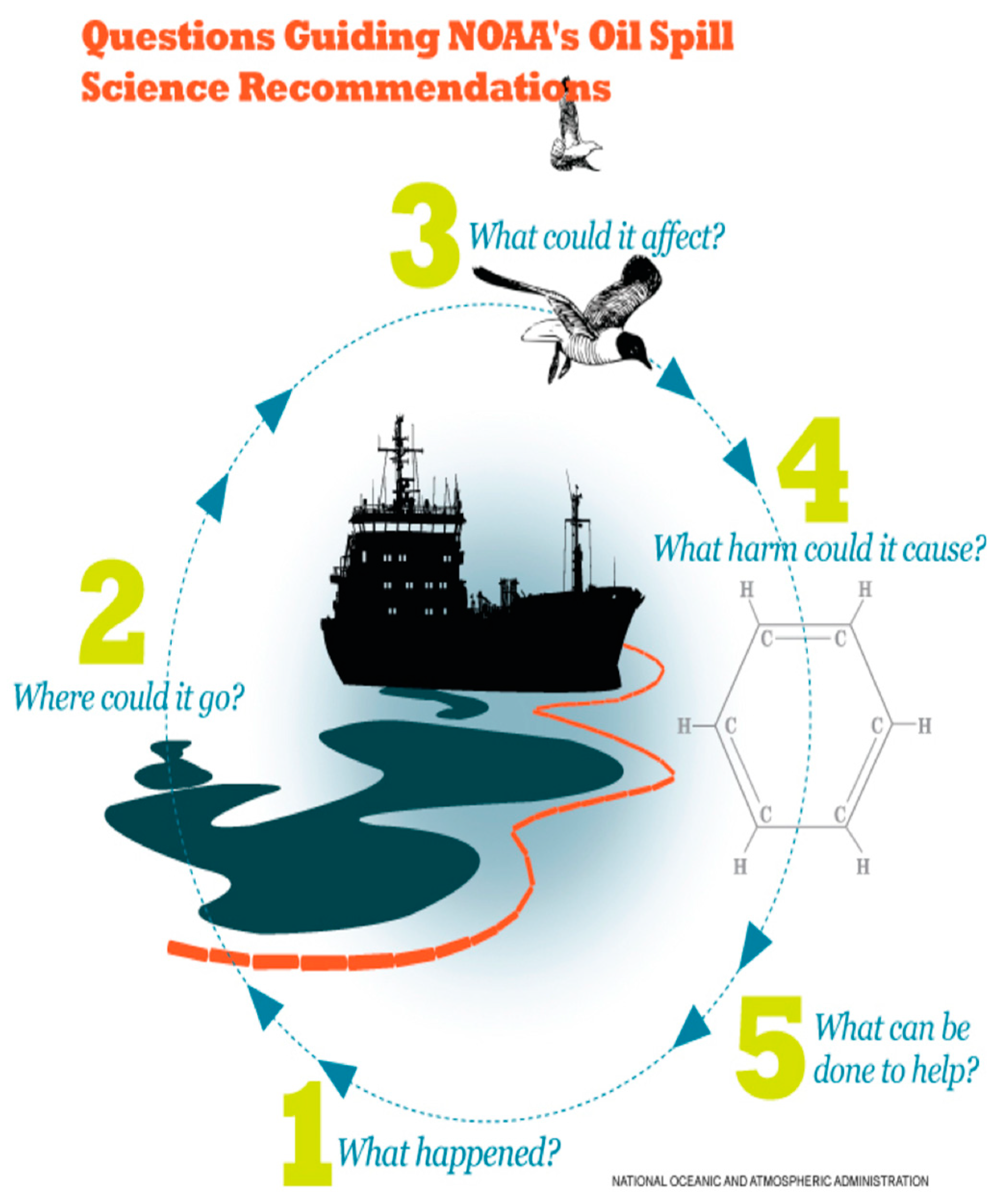
- (1)
- What Happened? In order to begin to plan a response, basic information needs to be available: How much oil was spilled? What type of oil? When was it spilled? Where was it spilled? Is there a continued release?
- (2)
- Where Could Oil Go? Once on the water, the oil will move—responders need to know where it might go in order to understand the potential impacts and know what response actions can be taken.
- (3)
- What Could the Spill Affect? What biota or ecosystems are present in the area where the oil might go?
- (4)
- What Harm Could the Spill Cause? Understanding the harm it could cause is critical for prioritizing response actions.
- (5)
- What Can Be Done to Help? Taking action to reduce the harm.
2. State of the Practice for Operational Oil Spill Modeling
2.1. Response Models
- (1)
- Gathering information about the spill: When, where, quantity, and characterization; collecting data from the “drivers”: Circulation models, meteorological models, and weather forecasts;
- (2)
- Evaluating these drivers for suitability for the case at hand;
- (3)
- Configuring the spill model;
- (4)
- Running the model;
- (5)
- Processing the output to present to responders, ideally with an evaluation of uncertainty.
2.2. Planning and Preparedness Models
2.3. Model Use Cases: Response Support
2.3.1. United States
U.S. Federal Operational Response Support
U.S. State Example (Texas)
2.3.2. Norway
2.3.3. Canada
2.3.4. Mediterranean Sea
2.3.5. International Industries
ITOPF
Oil Spill Response Limited (OSRL), United Kingdom
3. Earth System Modeling: Physical Drivers for Oil Spill Modeling
3.1. Ocean Circulation Modeling Component
3.1.1. Downscaling to High-Resolution Local Models
3.1.2. Challenges in Model Inputs
3.1.3. Representation of Important Ocean Processes: Sub-Mesoscale Features
3.1.4. Representation of Important Ocean Processes: Deep Ocean Currents
3.1.5. Observational Needs and Data Assimilation
3.1.6. Operational Issues
3.2. Meteorological/Wave Model Components
3.3. Coupling of Modeling Systems
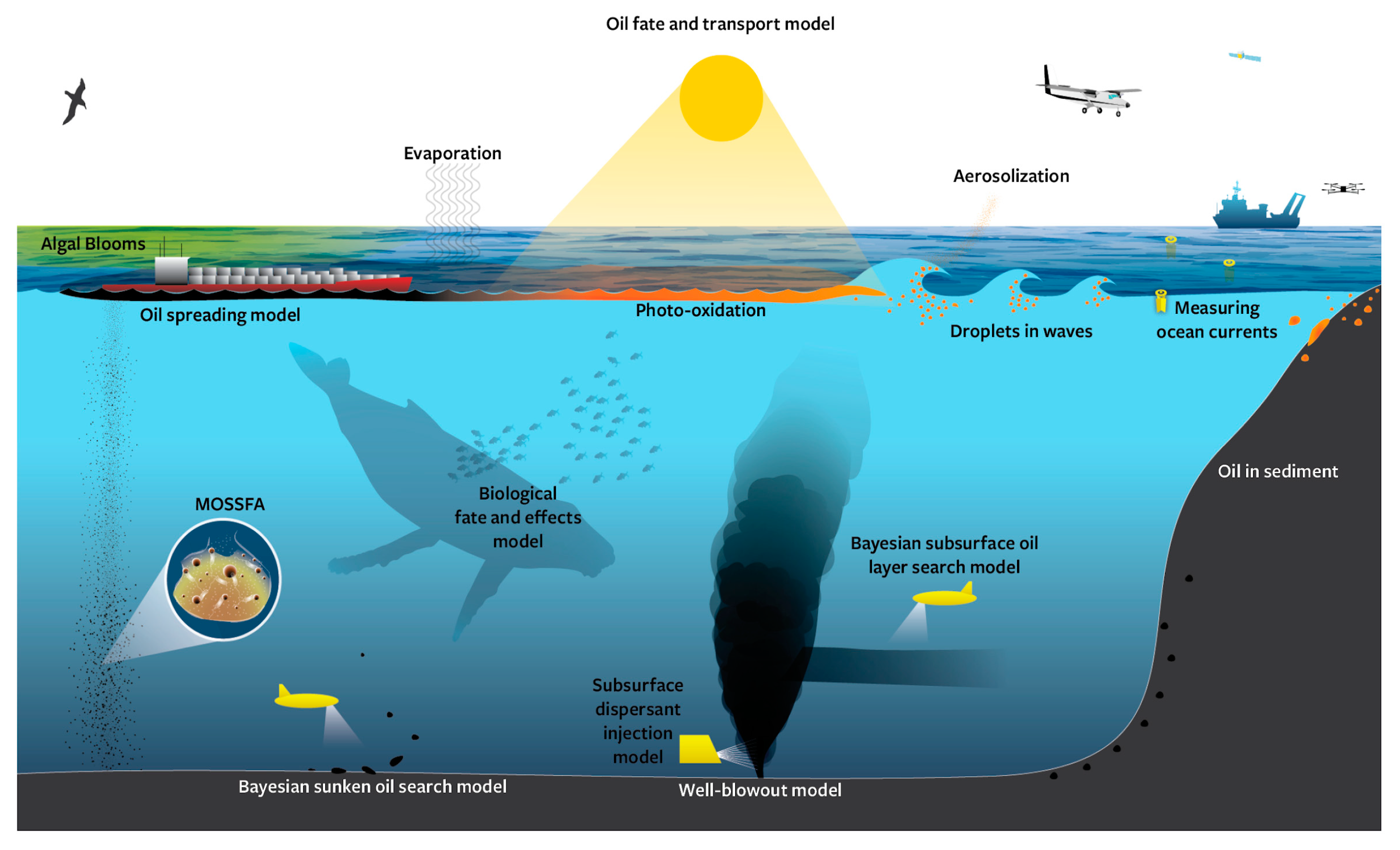
4. Oil Spill Modeling
4.1. Operational Considerations
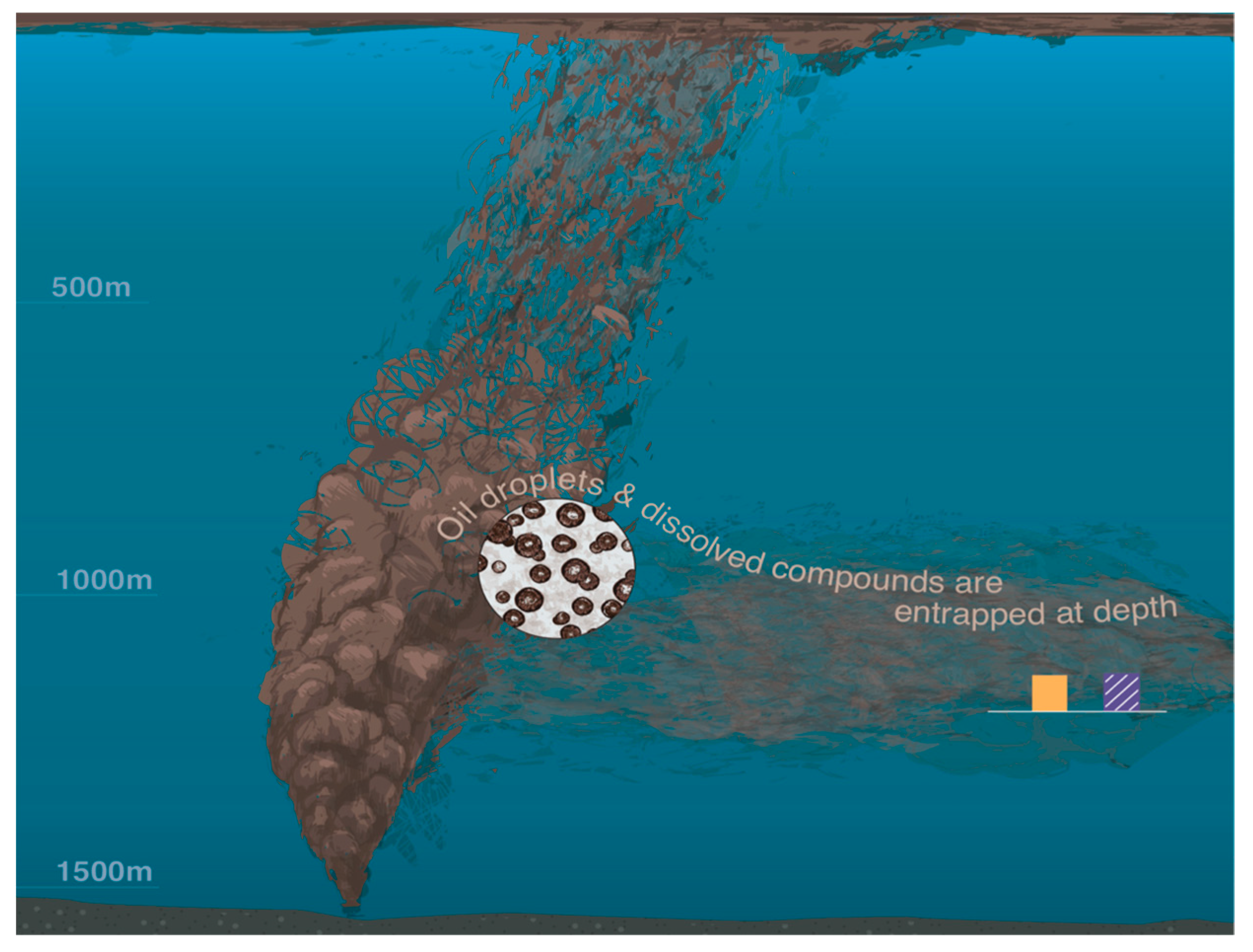
4.2. Subsea Plumes
4.2.1. Well Blow-Out Plume Modeling
4.2.2. Droplet Size
4.3. Processes in the Water Column
4.3.1. Dissolution
4.3.2. Degradation
4.3.3. Oxygen Demand
4.3.4. Marine Oil Snow Sedimentation and Flocculent Accumulation (MOSSFA)
4.4. Transport
4.4.1. Diffusion Parameterizations
4.4.2. Calculating Concentration
4.5. Surface Processes
4.5.1. Spreading
4.5.2. Entrainment
4.5.3. Weathering
4.5.4. Emulsion Formation
4.5.5. Photooxidation
5. Handling Uncertainty
5.1. Uncertainty in Ocean Circulation Models
5.2. Uncertainty in Oil Spill Models
5.3. Using More Observations to Reduce Uncertainty
5.4. Using Ensembles to Reduce Uncertainty
5.5. Communicating Uncertainty
6. Future Outlook
6.1. Improvements in Ocean Models
6.2. Improvements in Oil Models
6.2.1. More Data: Controlled Oil Release Experiments
6.2.2. Better Parameterizations: Transport
6.2.3. Better Parameterizations: Oil Fate
6.2.4. Better Parameterizations: Tarball Formation and Photooxidation
6.2.5. Better Parameterizations: MOSSFA
6.3. Improvements in Operations
Integration of Plume and Droplet Models
6.4. New Methodologies
6.4.1. Lagrangian Approaches
6.4.2. Lagrangian to Eulerian Transformation of Trajectory Model Point Distributions
6.4.3. Using Information Theory to Analyze Lagrangian Point Fields
6.4.4. Neural Networks and Artificial Intelligence
6.5. Toward a Comprehensive Approach on Operational Oil Spill Modeling
Author Contributions
Funding
Acknowledgments
Conflicts of Interest
Disclaimer
References
- Crone, T.J.; Tolstoy, M. Magnitude of the 2010 Gulf of Mexico oil leak. Sci. Express 2010, 330, 634. [Google Scholar] [CrossRef] [PubMed] [Green Version]
- Spaulding, M.L. State of the art review and future directions in oil spill modeling. Mar. Pollut. Bull. 2017, 115, 7–19. [Google Scholar] [CrossRef] [PubMed]
- French, D.P.; Schuttenberg, H.Z.; Isaji, T. Probabilities of Exceeding Thresholds of Concern: Examples from an Evaluation for Florida Power and Light. In Proceedings of the Twenty-Second Arctic and Marine Oil spill Program (AMOP) Technical Seminar, Calgary, AB, Canada, 2–4 June 1999; pp. 243–270. [Google Scholar]
- Aamo, O.E.; Reed, M.; Lewis, A. Regional Contingency Planning Using the OSCAR Oil Spill Contingency and Response Model. In Proceedings of the Twentieth Arctic and Marine Oil Spill Program (AMOP) Technical Seminar, Vancouver, BC, Canada, 11–13 June 1997. [Google Scholar]
- Barker, C.H.; Galt, J.A. Analysis of Methods used in Spill Response Planning: Trajectory Analysis Planner—TAP II. Spill Sci. Technol. Bull. 2000, 6, 145–152. [Google Scholar] [CrossRef]
- Boehm, P.D.; Page, D.S. Exposure Elements in Oil Spill Risk and Natural Resource Damage Assessment: A Review. Hum. Ecol. Risk Assess. Int. J. 2007. [Google Scholar] [CrossRef]
- Smith, R.A.; Slack, J.R.; Wyant, T.; Lanfear, K.J. The Oil Spill Risk Analysis Model of the U.S. Geological Survey. Reston (Virginia): U.S. Geological Survey. In U.S. Geological Survey Professional Paper 1227; The Branch of Distributio: Alexandria, VA, USA, 1982; p. 44. Available online: https://www.boem.gov/Environmental-Stewardship/Environmental-Assessment/Oil-Spill-Modeling/smithetal-pdf.aspx (accessed on 17 August 2020).
- MacFadyen, A.; Watabayashi, G.Y.; Barker, C.H.; Beegle-Krause, C.J. Tactical Modeling of Surface Oil Transport during the Deepwater Horizon Spill Response. In Monitoring and Modeling the Deepwater Horizon Oil Spill; Liu, A., MacFadyen, A., Ji, Z.-G., Weisberg, R.H., Eds.; John Wiley & Sons: Washington, DC, USA, 2011; pp. 167–178. [Google Scholar]
- Marcotte, G.; Bourgouin, P.; Mercier, G.; Gauthier, J.-P.; Pellerin, P.; Smith, G.; Onu, K.; Brown, C.E. Canadian Oil Spill Modelling Suite: An overview. In Proceedings of the 39th Arctic Marine Oil Spill Program Technical Seminar on Environmental Contamination and Response, Halifax, NS, Canada, 7–9 June 2016; pp. 1026–1034. [Google Scholar]
- Carpenter, A.; Donner, P.; Johansson, T. The Role of REMPEC in Prevention of and Response to Pollution from Ships in the Mediterranean Sea. In Oil Pollution in the Mediterranean Sea: Part, I. The Handbook of Environmental Chemistry; Carpenter, A., Kostianoy, A., Eds.; Springer: Berlin/Heidelberg, Germany, 2017; pp. 167–190. [Google Scholar]
- Girin, M.; Carpenter, A. Shipping and Oil Transportation in the Mediterranean Sea. In Oil Pollution in the Mediterranean Sea: Part I; Springer: Berlin/Heidelberg, Germany, 2017; pp. 33–51. [Google Scholar]
- Zodiatis, G.; Coppini, G.; Perivoliotis, L.; Lardner, R.; Alves, T.; Pinardi, N.; Liubartseva, S.; De Dominicis, M.; Bourma, E.; Sepp Neves, A.A. Numerical Modeling of Oil Pollution in the Eastern Mediterranean Sea. In Oil Pollution in the Mediterranean Sea: Part, I. The Handbook of Environmental Chemistry; Carpenter, A., Kostianoy, A., Eds.; Springer: Berlin/Heidelberg, Germany, 2017; Volume 83, pp. 215–254. [Google Scholar]
- Cucco, A.; Daniel, P. Numerical Modeling of Oil Pollution in the Western Mediterranean Sea. In Oil Pollution in the Mediterranean Sea: Part, I. The Handbook of Environmental Chemistry; Carpenter, A., Kostianoy, A., Eds.; Springer: Berlin/Heidelberg, Germany, 2016; Volume 83, pp. 255–271. [Google Scholar]
- Pinardi, N.; Cavaleri, L.; Coppini, G.; De Mey, P.; Fratianni, C.; Huthnance, J.; Lermusiaux, P.E.; Navarra, A.; Preller, R.; Tibaldi, S. From weather to ocean predictions: An historical viewpoint. J. Mar. Res. 2017, 75, 103–159. [Google Scholar] [CrossRef] [Green Version]
- Le Traon, P.Y.; Reppucci, A.; Alvarez Fanjul, E.; Aouf, L.; Behrens, A.; Belmonte, M.; Bentamy, A.; Bertino, L.; Brando, V.E.; Kreiner, M.B.; et al. From Observation to Information and Users: The Copernicus Marine Service Perspective. Front. Mar. Sci. 2019, 6, 234. [Google Scholar] [CrossRef] [Green Version]
- Tintorè, J.; Pinardi, N.; Álvarez-Fanjul, E.; Aguiar, E.; Álvarez-Berastegui, D.; Bajo, M.; Balbin, R.; Bozzano, B.; Buongiorno Nardelli, B.; Cardin, V.; et al. Challenges for Sustained Observing and Forecasting Systems in the Mediterranean Sea. Front. Mar. Sci. 2019, 6. [Google Scholar] [CrossRef] [Green Version]
- Daniel, P. Operational forecasting of oil spill drift at Météo-France. Spill Sci. Technol. Bull. 1996, 3, 53–64. [Google Scholar] [CrossRef] [Green Version]
- Lardner, R.W.; Zodiatis, G.; Loizides, L.; Demetropoulos, A. An operational oil-spill model for the Levantine Basin (Eastern Mediterranean Sea). In Proceedings of the International Symposium on Marine Pollution, Monaco, 5–9 October 1998; pp. 511–512. [Google Scholar]
- De Dominicis, M.; Pinardi, N.; Zodiatis, G.; Lardner, R. MEDSLIK-II, a Lagrangian marine surface oil spill model for short-term forecasting—Part 1: Theory. Geosci. Model Dev. 2013, 6, 1851–1869. [Google Scholar] [CrossRef] [Green Version]
- Pollani, A.; Triantafyllou, G.; Petihakis, G.; Nittis, K.; Dounas, C.; Koutitas, C. The Poseidon Operational Tool for the Prediction of Floating Pollutant Transport. Mar. Pollut. Bull. 2001, 43, 270–278. [Google Scholar] [CrossRef]
- Coppini, G.; De Dominicis, M.; Zodiatis, G.; Lardner, R.; Pinardi, N.; Santoleri, R.; Colella, S.; Bignami, F.; Hayes, D.R.; Soloviev, D.; et al. Hindcast of oil-spill pollution during the Lebanon crisis in the Eastern Mediterranean, July–August 2006. Mar. Pollut. Bull. 2011. [Google Scholar] [CrossRef] [PubMed]
- De Dominicis, M.; Bruciaferri, D.; Gerin, R.; Pinardi, N.; Poulain, P.M.; Garreau, P.; Zodiatis, G.; Perivoliotis, L.; Fazioli, L.; Sorgente, R.; et al. A multi-model assessment of the impact of currents, waves and wind in modelling surface drifters and oil spill. Deep-Sea Res. II 2016, 133, 21–38. [Google Scholar] [CrossRef] [Green Version]
- Zodiatis, G.; De Dominicis, M.; Perivoliotis, L.; Radhakrishnan, H.; Georgoudis, E.; Sotillo, M.; Lardner, R.W.; Krokos, G.; Bruciaferri, D.; Clementi, E.; et al. The Mediterranean Decision Support System for Marine Safety dedicated to oil slicks predictions. Deep-Sea Res. II 2016. [Google Scholar] [CrossRef]
- Schiller, A.; Mourre, B.; Drillet, Y.; Brassington, G. An overview of operational oceanography. In New Frontiers in Operational Oceanography; Chassignet, E., Pascual, A., Tintoré, J., Verron, J., Eds.; GODAE Ocean View; The Florida State University Libraries: Tallahassee, FL, USA, 2018; pp. 1–26. [Google Scholar] [CrossRef] [Green Version]
- Ford, D.; Kay, S.; McEwan, R.; Totterdell, I.; Gehlen, M. Marine biogeochemical modelling and data assimilation for operational forecasting, reanalysis and climate research. In New Frontiers in Operational Oceanography; Chassignet, E., Pascual, A., Tintoré, J., Verron, J., Eds.; GODAE Ocean View; The Florida State University Libraries: Tallahassee, FL, USA, 2018; pp. 625–652. [Google Scholar] [CrossRef] [Green Version]
- Chassignet, E.P.; Hurlburt, H.E.; Smedstad, O.M.; Halliwell, G.R.; Hogan, P.J.; Wallcradt, A.J.; Baraille, R.; Bleck, R. The HYCOM (Hybrid Coordinate Ocean Model) data assimilative system. J. Mar. Syst. 2007, 65, 60–83. [Google Scholar] [CrossRef]
- Mariano, A.J.; Kourafalou, V.H.; Srinivasan, A.; Kang, H.; Halliwell, G.R.; Ryan, E.H.; Roffer, M. On the modeling of the 2010 Gulf of Mexico Oil Spill. Dynam. Atmos. Ocean 2011, 52, 322–340. [Google Scholar] [CrossRef]
- Le Hénaff, M.; Kourafalou, V.H.; Paris, C.B.; Helgers, J.; Hogan, P.J.; Srinivasan, A. Surface evolution of the Deepwater Horizon oil spill: Combined effects of circulation and wind induced drift. Environ. Sci. Technol. 2012, 46, 7267–7273. [Google Scholar] [CrossRef]
- Hyun, K.H.; He, R. Coastal upwelling in the South Atlantic Bight: A revisit of the 2003 cold event using long term observations and model hindcast solutions. J. Mar. Syst. 2010, 839, 1–13. [Google Scholar] [CrossRef]
- Mehra, A.; Rivin, I. A real time ocean forecast system for the North Atlantic Ocean. Terr. Atmos. Ocean. Sci. 2010, 21, 211–228. [Google Scholar] [CrossRef] [Green Version]
- Ko, D.S.; Martin, P.J.; Rowley, C.D.; Preller, R.H. A real-time coastal ocean prediction experiment for MREA04. J. Mar. Syst. 2008, 69, 17–28. [Google Scholar] [CrossRef]
- Barth, A.; Alvera-Azcárate, A.; Weisberg, R.H. A nested model study of the Loop Current generated variability and its impact on the West Florida Shelf. J. Geophys. Res. 2008, 113, C05009. [Google Scholar] [CrossRef]
- Fox-Kemper, B.; Adcroft, A.; Böning, C.W.; Chassignet, E.P.; Curchitser, E.; Danabasoglu, G.; Eden, C.; England, M.H.; Gerdes, R.; Greatbatch, R.J.; et al. Challenges and prospects in ocean circulation models. Front. Mar. Sci. 2019, 6, 65. [Google Scholar] [CrossRef]
- Chassignet, E.P.; Xu, X. Impact of horizontal resolution (1/12 to 1/50) on Gulf Stream separation, penetration, and variability. J. Phys. Oceanogr. 2017, 47, 1999–2021. [Google Scholar] [CrossRef]
- Le Hénaff, M.; Kourafalou, V.H. Mississippi waters reaching South Florida reefs under no flood conditions: Synthesis of observing and modeling system findings. Ocean Dyn. 2016, 66, 435–459. [Google Scholar] [CrossRef]
- Jacobs, G.; DAddezio, J.; Bartels, B.; Spence, P. Constrained scales in ocean forecasting. Adv. Space Res. 2019. [Google Scholar] [CrossRef]
- Capet, X.; McWilliams, J.C.; Molemaker, M.J.; Shchepetkin, A.F. Mesoscale to Sub-mesoscale Transition in the California Current System. Part I: Flow Structure, Eddy Flux, and Observational Tests. J. Phys. Oceanogr. 2008, 38, 29–43. [Google Scholar] [CrossRef] [Green Version]
- Kourafalou, V.H.; De Mey, P.; Staneva, J.; Ayoub, N.; Barth, A.; Chao, Y.; Cirano, M.; Fiechter, J.; Herzfeld, M.; Kurapov, A.; et al. Coastal Ocean Forecasting: Science foundation and user benefits. J. Oper. Oceangr. 2015. [Google Scholar] [CrossRef]
- Kourafalou, V.H.; De Mey, P.; Le Hénaff, M.; Charria, G.; Edwards, C.A.; He, R.; Herzfeld, M.; Pasqual, A.; Stanev, E.; Tintoré, J.; et al. Coastal Ocean Forecasting: System integration and validation. J. Oper. Oceangr. 2015. [Google Scholar] [CrossRef] [Green Version]
- Wilkin, J.L.; Hunter, E.J. An assessment of the skill of real-time models of Mid-Atlantic Bight continental shelf circulation. J. Geophys. Res. Ocean. 2013, 118, 2919–2933. [Google Scholar] [CrossRef]
- Kourafalou, V.H.; Oey, L.-Y.; Wang, J.D.; Lee, T.N. The fate of river discharge on the continental shelf. Part I: Modeling the river plume and the inner-shelf coastal current. J. Geophys. Res. 1996, 101, 3415–3434. [Google Scholar] [CrossRef]
- Schiller, R.V.; Kourafalou, V.H. Modeling river plume dynamics with the Hybrid Coordinate Ocean Model. Ocean Model 2010. [Google Scholar] [CrossRef]
- Kourafalou, V.H.; Oey, L.-Y.; Lee, T.N.; Wang, J.D. The fate of river discharge on the continental shelf. Part II: Transport of low-salinity waters under realistic wind and tidal forcing. J. Geophys. Res. 1996, 101, 3435–3455. [Google Scholar] [CrossRef]
- Tseng, Y.-H.; Bryan, F.O.; Whitney, M.M. Impacts of the representation of riverine freshwater input in the Community Earth System Model. Ocean Model 2016, 105, 71–86. [Google Scholar] [CrossRef] [Green Version]
- Le Hénaff, M.; Muller-Karger, F.E.; Kourafalou, V.H.; Otis, D.; Johnson, K.A.; McEachron, L.; Kang, H. Coral Mortality in the Flower Garden Banks of the Gulf of Mexico in July 2016: The Consequence of Cross-Shelf Transport of Flood Waters? Cont. Shelf Res. 2019, 190. [Google Scholar] [CrossRef]
- Kourafalou, V.H.; Androulidakis, Y.S. Influence of Mississippi induced circulation on the Deepwater Horizon Oil Spill transport. J. Geophys. Res. 2013, 118, 1–20. [Google Scholar] [CrossRef]
- Androulidakis, I.; Kourafalou, V.; Özgökmen, T.M.; Garcia-Pineda, O.; Lund, B.; Henaff, M.L.; Hu, C.; Haus, B.K.; Novelli, G.; Guigand, C.; et al. Influence of river induced fronts on hydrocarbon transport: A multi-platform observational study. J. Geophys. Res. Oceans 2018, 123, 3259–3285. [Google Scholar] [CrossRef] [Green Version]
- Hole, L.; Dagestad, K.F.; Röhrs, J.; Wettre, C.; Kourafalou, V.H.; Androulidakis, Y.S.; Le Hénaff, M.; Kang, H.; Garcia, O. Revisiting the DeepWater Horizon spill: High resolution model simulations of effects of oil droplet size distribution and river fronts. J. Mar. Sci. Eng. 2019, 7, 329. [Google Scholar] [CrossRef] [Green Version]
- Androulidakis, Y.S.; Kourafalou, V.H.; Le Hénaff, M.; Kang, H.; Sutton, T.; Chen, S.; Hu, C.; Ntaganou, N. Offshore spreading of Mississippi waters: Pathways and vertical structure under eddy influence. J. Geophys. Res. 2019, 124. [Google Scholar] [CrossRef]
- Poje, A.C.; Özgökmen, T.M.; Lipphart, B., Jr.; Haus, B.; Ryan, E.; Haza, A.; Jacobs, G.; Reniers, A.; Olascoaga, J.; Novelli, G.; et al. Sub-mesoscale dispersion in the vicinity of the Deepwater Horizon spill. Proc. Natl. Acad. Sci. USA 2014, 11135, 12693–12698. [Google Scholar] [CrossRef] [Green Version]
- Haza, A.C.; Özgökmen, T.; Griffa, A.; Garraffo, Z.D.; Piterbarg, L. Parameterization of particle transport at sub-mesoscales in the Gulf Stream region using Lagrangian subgrid scale models. Ocean Model 2012, 42, 31–49. [Google Scholar] [CrossRef]
- Haza, A.C.; Özgökmen, T.; Hogan, P. Impact of sub-mesoscales on surface material distribution in a Gulf of Mexico mesoscale eddy. Ocean Model 2016, 107, 28–47. [Google Scholar] [CrossRef] [Green Version]
- Huguenard, K.; Bogucki, D.J.; Ortiz-Suslow, D.G.; Laxague, N.J.M.; MacMahan, J.H.; Özgökmen, T.M.; Haus, B.K.; Reniers, A.J.H.M.; Hargrove, J.; Soloviev, A.V.; et al. On the nature of the frontal zone of the Chactawhatchee Bay plume in the Gulf of Mexico. J. Geophys. Res. Ocean. 2016, 121, 1322–1345. [Google Scholar] [CrossRef] [Green Version]
- Roth, M.; MacMahan, J.; Reniers, A.; Özgökmen, T.; Woodall, K.; Haus, B. Observations of inner shelf cross-shore surface material transport adjacent to a coastal inlet in the northern Gulf of Mexico. Cont. Shelf Res. 2017, 137, 142–153. [Google Scholar] [CrossRef]
- Rascle, N.; Molemaker, J.; Mari, L.; Nouguier, F.; Chapron, B.; Lund, B.; Mouche, A. Intense deformation field at oceanic front inferred from directional sea surface roughness observations. Geophys. Res. Lett. 2017, 44, 5599–5608. [Google Scholar] [CrossRef] [Green Version]
- D’Asaro, E.; Shcherbina, A.; Klymak, J.; Molemaker, J.; Novelli, G.; Guigand, C.; Haza, A.; Haus, B.; Ryan, E.; Jacobs, G.; et al. Ocean convergence and dispersion of flotsam. Proc. Natl. Acad. Sci. USA 2018, 115, 1162–1167. [Google Scholar]
- Haza, A.C.; Paldor, N.; Özgökmen, T.; Curcic, M.; Chen, S.S.; Jacobs, G. Wind-based estimations of ocean surface currents from massive clusters of drifters in the Gulf of Mexico. J. Geophys. Res. Ocean. 2019, 124, 5844–5869. [Google Scholar] [CrossRef]
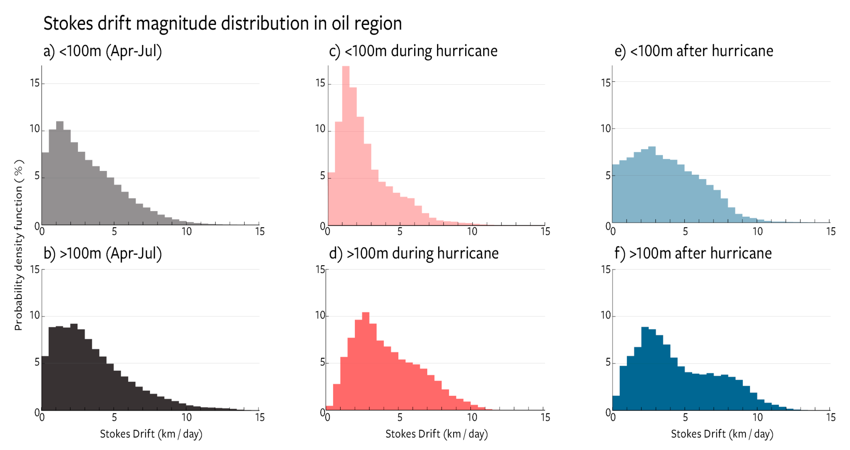
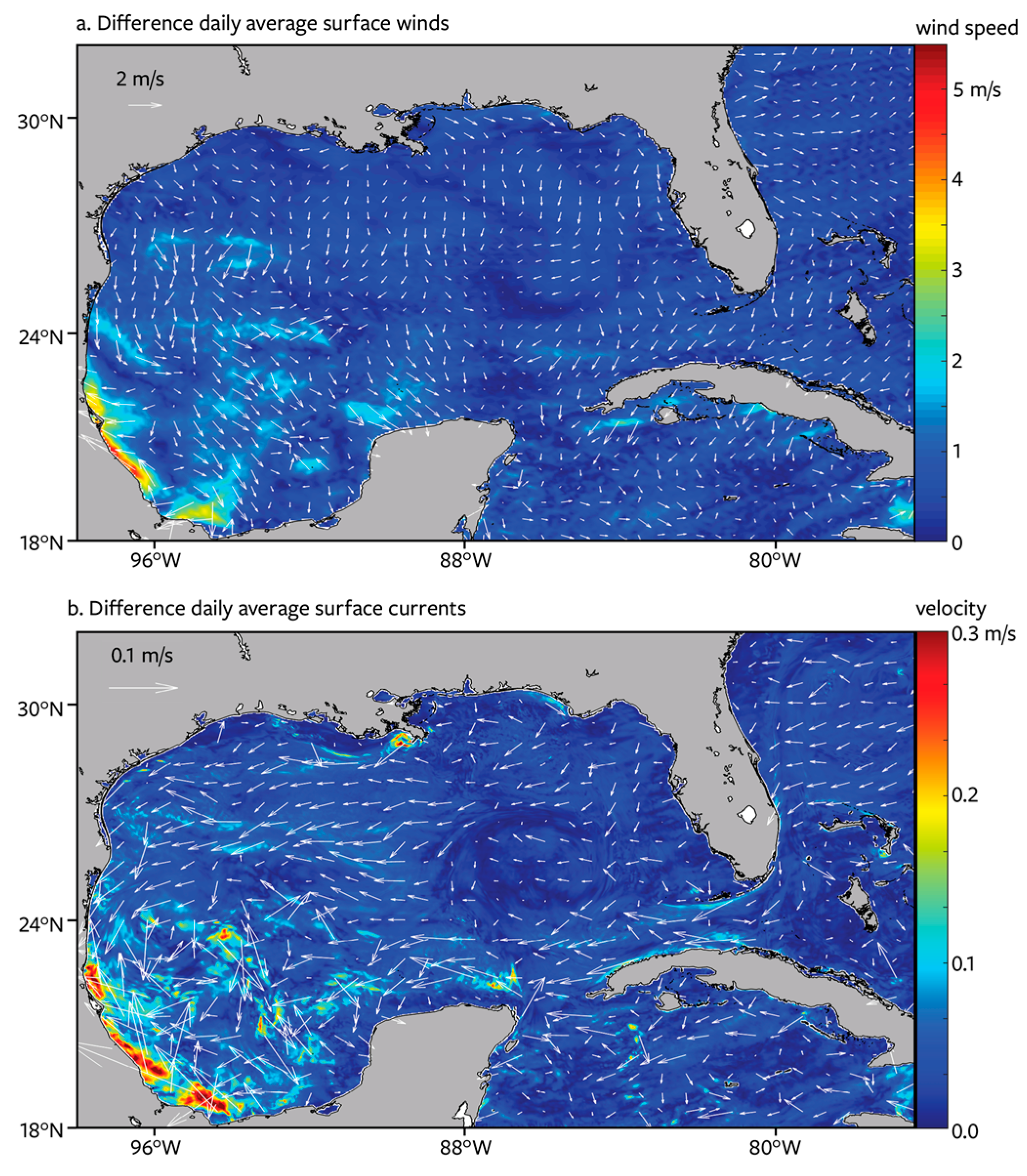
- Curcic, M.; Chen, S.; Özgökmen, T.M. Hurricane-induced ocean waves and Stokes drift and their impacts on surface transport and dispersion in the Gulf of Mexico. Geophys. Res. Lett. 2016, 43, 2773–2781. [Google Scholar] [CrossRef]
- Laxague, N.J.M.; Özgökmen, T.M.; Haus, B.K.; Novelli, G.; Shcherbina, A.; Sutherland, P.; Guigand, C.; Lund, B.; Mehta, S.; Alday, M.; et al. Observations of near-surface current shear help describe oceanic oil and plastic transport. Geophys. Res. Letts. 2018, 45, 245–249. [Google Scholar] [CrossRef] [Green Version]
- Morey, S.; Gopalakrishnan, S.; Pallas Sanz, E.; Marcos Azevedo Correia De Souza, J.; Donohue, K.; Perez-Brunius, P.; Dukhovskoy, D.; Chassignet, E.P.; Cornuelle, B.; Bower, A.; et al. Assessment of numerical simulations of deep circulation and variability in the Gulf of Mexico using recent observations. J. Phys. Oceanogr. 2020. [Google Scholar] [CrossRef]
- Ogle, M.T.; Smith, R.; Williams, B.; Schiller, R.; Perry, R.; Leung, P.; DiMarco, S.F.; Howden, S. Four Years of Metocean Support to the Shell Stones Field: From Asset Integrity to Collaborative Research. In Proceedings of the Offshore Technology Conference, Houston, TX, USA, 6–9 May 2019. [Google Scholar] [CrossRef]
- Barkan, R.; McWilliams, J.C.; Shchepetkin, A.F.; Molemaker, M.J.; Renault, L.; Bracco, A.; Choi, J. Sub-mesoscale dynamics in the northern Gulf of Mexico. Part I: Regional and seasonal characterization and the role of river outflow. J. Phys. Oceanogr. 2017, 47, 2325–2346. [Google Scholar] [CrossRef]
- Shi, Q.; Bourassa, M.A. Coupling Ocean Currents and Waves with Wind Stress over the Gulf Stream. Remote Sens. 2019, 11, 1476. [Google Scholar] [CrossRef] [Green Version]
- Smith, S.; Cummings, J.; Rowley, C.; Chu, P.; Shriver, J.; Helber, R.; Spence, P.; Carroll, S.; Smedstad, O.; Lunde, B. Validation Test Report for the Navy Coupled Ocean Data Assimilation 3D Variational Analysis (NCODA-VAR) System; Version 3.43 Rep.; NRL Report NRL/MR/7320-11-9363; Naval Research Laboratory, Stennis Space Center: Hancock County, MS, USA, 2011. [Google Scholar]
- Smith, S.; Ngodock, H.; Carrier, M.; Shriver, J.; Muscarella, P.; Souopgui, I. Validation and Operational Implementation of the Navy Coastal Ocean Model Four Dimensional Variational Data Assimilation System (NCOM 4DVAR) in the Okinawa Trough. in Data Assimilation for Atmospheric, Oceanic and Hydrologic Applications (Vol. III), Edited; Springer: Berlin/Heidelberg, Germany, 2017; pp. 405–427. [Google Scholar]
- Jacobs, G.A.; Bartels, B.P.; Bogucki, D.J.; Beron-Vera, F.J.; Chen, S.S.; Coelho, E.F.; Curcic, M.; Griffa, A.; Gough, M.; Haus, B.K. Data assimilation considerations for improved ocean predictability during the Gulf of Mexico Grand Lagrangian Deployment (GLAD). Ocean Model 2014, 83, 98–117. [Google Scholar] [CrossRef]
- D’Addezio, J.M.; Jacobs, G.A.; Yaremchuk, M.; Souopgui, I. Sub-mesoscale Eddy Vertical Covariances and Dynamical Constraints from High-Resolution. J. Phys. Oceanogr. 2020, 50, 1087–1115. [Google Scholar] [CrossRef] [Green Version]
- Carrier, M.J.; Ngodock, H.E.; Muscarella, P.; Smith, S. Impact of assimilating surface velocity observations on the model sea surface height using the NCOM-4DVAR. Mon. Weather Rev. 2016, 144, 1051–1068. [Google Scholar] [CrossRef]
- Muscarella, P.; Carrier, M.J.; Ngodock, H.; Smith, S.; Lipphardt, B., Jr.; Kirwan, A., Jr.; Huntley, H.S. Do assimilated drifter velocities improve Lagrangian predictability in an operational ocean model? Mon. Weather Rev. 2015, 143, 1822–1832. [Google Scholar] [CrossRef]
- Rodríguez, E.; Wineteer, A.; Perkovic-Martin, D.; Gál, T.; Stiles, B.W.; Niamsuwan, N.; Rodriguez Monje, R. Estimating Ocean Vector Winds and Currents Using a Ka-Band Pencil-Beam Doppler Scatterometer. Remote Sens. 2018, 10, 576. [Google Scholar] [CrossRef] [Green Version]
- Rodríguez, E.; Bourassa, M.; Chelton, D.; Farrar, J.T.; Long, D.; Perkovic-Martin, D.; Samelson, R. The Winds and Currents Mission Concept. Front. Mar. Sci. 2019, 6, 438. [Google Scholar] [CrossRef]
- Zheng, Y.; Bourassa, M.A.; Hughes, P.J. Influences of sea surface temperature gradients and surface roughness changes on the motion of surface oil: A simple idealized study. J. Appl. Meteor. Clim. 2013, 52, 1561–1575. [Google Scholar] [CrossRef]
- Liu, Y.; MacFadyen, A.; Ji, Z.-G.; Weisberg, R.H. Monitoring and Modeling the Deepwater Horizon Oil Spill: A Record Breaking Enterprise. Geophysical Monograph; American Geophysical Union: Washington, DC, USA, 2011; p. 195. [Google Scholar]
- Weber, J.E. Friction-induced roll motion in short-crested surface gravity waves. J. Phys. Oceanogr. 1985, 15, 936–942. [Google Scholar] [CrossRef] [Green Version]
- O’Neil, L.W.; Chelton, D.B.; Esbensen, S.K. Covariability of surface winds and stress responses to sea surface temperature ronts. J. Clim. 2012, 25, 5916–5942. [Google Scholar] [CrossRef] [Green Version]
- Song, Q.; Chelton, D.B.; Esbensen, S.K.; Thum, N.; O’Neill, L.W. Coupling between sea surface temperature and low-level winds in mesoscale numerical models. J. Clim. 2009, 22, 146–164. [Google Scholar] [CrossRef]
- Nakanishi, M.; Niino, H. An improved Mellor-Yamada level-3 model with condensation physics: Its design and verification. Bound. Layer. Meteor. 2004, 112, 1–31. [Google Scholar] [CrossRef]
- Grenier, H.; Bretherton, C.S. A moist PBL parameterization for large-scale models and its application to subtropical cloud-topped marine boundary layers. Mon. Weather Rev. 2001, 129, 357–377. [Google Scholar] [CrossRef] [Green Version]
- Judt, F.; Chen, S.S.; Curcic, M. Atmospheric forcing of the upper ocean transport in the Gulf of Mexico from seasonal to diurnal scales. J. Geophys. Res. Ocean. 2016, 121, 4416–4433. [Google Scholar] [CrossRef] [Green Version]
- Rowley, C.; Mask, A. Regional and coastal prediction with the relocatable ocean nowcast/forecast system. Oceanography 2014, 27, 44–55. [Google Scholar] [CrossRef] [Green Version]
- Allard, R.; Rogers, E.; Martin, P.; Jensen, T.; Chu, P.; Campbell, T.; Dykes, J.; Smith, T.; Choi, J.; Gravois, U. The US Navy coupled ocean-wave prediction system. Oceanography 2014, 27, 92–103. [Google Scholar] [CrossRef]
- Galt, J.A. Trajectory Analysis for Oil Spills. J. Adv. Mar. Technol. Conf. 1994, 11, 91–126. [Google Scholar]
- French McCay, D.P.; Jayko, K.; Li, Z.; Horn, M.; Kim, Y.; Isaji, T.; Crowley, D.; Spaulding, M.; Decker, L.; Turner, C.; et al. Technical Reports for Deepwater Horizon Water Column Injury Assessment—WC_TR14: Modeling Oil Fate and Exposure Concentrations in the Deepwater Plume and Cone of Rising Oil Resulting from the Deepwater Horizon Oil Spill. DWH NRDA Water Column Technical Working Group Report. Prepared for National Oceanic and Atmospheric Administration by RPS ASA, South Kingstown, RI, USA, 29 September 2015, Administrative Record no. DWH-AR0285776.pdf. Available online: https://www.doi.gov/deepwaterhorizon/adminrecord (accessed on 28 August 2020).
- French McCay, D.P.; Morandi, A.; McManus, M.C.; Schroeder, M.; Jayko, K.; Rowe, J.J. Technical Reports for Deepwater Horizon Water Column Injury Assessment—WC_TR.09: Vertical Distribution Analysis of Plankton. DWH NRDA Water Column Technical Working Group Report. Prepared for National Oceanic and Atmospheric Administration by RPS ASA, South Kingstown, RI, USA. DWH NRDA Water Column Technical Working Group Report. Prepared for National Oceanic and Atmospheric Administration by RPS ASA, South Kingstown, RI, USA, Administrative Record no. DWH-AR0195958.pdf, DWH-AR0171921.xlsx, DWH-AR0171922.xlsx, 2015b. Available online: https://www.doi.gov/deepwaterhorizon/adminrecord (accessed on 28 August 2020).
- French McCay, D.P.; McManus, M.C.; Balouskus, R.; Rowe, J.J.; Schroeder, M.; Morandi, A.; Bohaboy, E.; Graham, E. Technical Reports for Deepwater Horizon Water Column Injury Assessment: WC_TR.10: Evaluation of Baseline Densities for Calculating Direct Injuries of Aquatic Biota During the Deepwater Horizon Oil Spill. DWH NRDA Water Column Technical Working Group Report. Prepared for National Oceanic and Atmospheric Administration by RPS ASA, South Kingstown, RI, USA, Administrative Record no. DWH-AR0285021.pdf, DWH-AR0285141.xlsx, DWH-AR02851412.xlsx, 2015c. Available online: https://www.doi.gov/deepwaterhorizon/adminrecord (accessed on 28 August 2020).
- French McCay, D.P.; Li, Z.; Horn, M.; Crowley, D.; Spaulding, M.; Mendelsohn, D.; Turner, C. Modeling Oil Fate and Subsurface Exposure Concentrations from the Deepwater Horizon Oil Spill. In Proceedings of the 39th AMOP Technical Seminar on Environmental Contamination and Response, Halifax, NS, Canada, 7–9 June 2016; Volume 39, pp. 115–150. [Google Scholar]
- Yang, D.; Chen, B.; Socolofsky, S.; Chamecki, M.; Meneveau, C. Large-eddy simulation and parameterization of buoyant plume dynamics in stratified flow. J. Fluid Mech. 2016, 794, 798–833. [Google Scholar] [CrossRef]
- Fabregat, A.; Poje, A.; Ozgokmen, T.; Dewar, W.K. Numerical simulations of rotating bubble plumes in stratified environments. J. Geophys. Res. Ocean. 2017, 10, 6795–6813. [Google Scholar] [CrossRef]
- Fabregat, A.; Deremble, B.; Wienders, N.; Stroman, A.; Poje, A.; Ozgokmen, T.; Dewar, W.K. Rotating 2d Point Source Plume Models with Application to Deep Water Horizon. Ocean Model 2017, 119, 118–135. [Google Scholar] [CrossRef]
- Breivik, Ø.; Allen, A.A.; Maisondieu, C.; Olangnon, M. Advances in search and rescue at sea. Ocean Dyn. 2013, 63, 83–88. [Google Scholar] [CrossRef] [Green Version]
- Garcia-Pineda, O.; Staples, G.; Jones, C.E.; Hu, C.; Holt, B.; Kourafalou, V.H.; Haces-Garcia, F. Classification of oil spill by thicknesses using multiple remote sensors. Remote Sens. Environ. 2020, 236. [Google Scholar] [CrossRef]
- Garcia-Pineda, O.; Androulidakis, Y.; Le Henaff, M.; Kourafalou, V.H.; Hole, L.R.; Kang, H.; DiPinto, L. Measuring oil residence time with GPS-drifters, satellites, and Unmanned Aerial Systems (UAS). Mar. Pollut. Bull. 2020, 150, 110644. [Google Scholar] [CrossRef] [PubMed]
- Barker, C.H.; MacFadyen, A. WebGNOME Additions for Remote Sensing Ingestion for Model Initialization. In Interagency Agreement: E19PG00023 between the Bureau of Safety and Environmental Enforcement and the National Oceanic and Atmospheric Administration; Bureau of Safety: Washington, DC, USA; National Oceanic: Silver Spring, MD, USA; Atmospheric Administration: Silver Spring, MD, USA, 2019. [Google Scholar]
- Jacketti, M.; Ji, C.; Englehardt, J.D.; Beegle-Krause, C. Development of the SOSIM Model for Inferential Tracking of Subsurface Oil. In Proceedings of the Arctic and Marine Oil Pollution Conference, Environment and Climate Change Canada, Halifax, NS, Canada, 4–6 June 2019; pp. 485–501. [Google Scholar]
- French-McCay, D.; Horn, M.; Li, Z.; Jayko, K.; Spaulding, M.; Crowley, D.; Mendelsohn, D. Modeling Distribution Fate and Concentrations of Deepwater Horizon Oil in Subsurface Waters of the Gulf of Mexico. Chapter 31. In Oil Spill Environmental Forensics Case Studies; Stout, S., Wang, Z., Eds.; Butterworth-Heinemann: Oxford, UK, 2018; pp. 683–736. ISBN 978-O-12-804434-6. [Google Scholar]
- French-McCay, D.; Crowley, D.; Rowe, J.; Bock, M.; Robinson, H.; Wenning, R.; Walker, A.H.; Joeckel, J.; Parkerton, T. Comparative Risk Assessment of Spill Response Options for a Deepwater Oil Well Blowout: Part, I. Oil Spill Modeling. Mar. Pollut. Bull. 2018, 133, 1001–1015. [Google Scholar] [CrossRef] [PubMed]
- Yapa, P.D.; Dasanayaka, L.K.; Bandara, U.C.; Nakata, K. A model to simulate the transport and fate of gas and hydrates released in deepwater. J. Hydraul. Res. 2010, 48, 559–572. [Google Scholar] [CrossRef]
- Johansen, Ø. Development and verification of deep-water blowout models. Mar. Pollut. Bull. 2003, 47, 360–368. [Google Scholar] [CrossRef]
- Dissanayake, A.L.; Gros, J.; Socolofsky, S.A. Integral models for bubble, droplet, and multiphase plume dynamics in stratification and crossflow. Environ. Fluid Mech. 2018, 18, 1167–1202. [Google Scholar] [CrossRef] [Green Version]
- Bombardelli, F.A.; Buscaglia, G.C.; Rehmann, C.R.; Rincon, L.E.; Garcia, M.H. Modeling and scaling of aeration bubble plumes: A two-phase flow analysis. J. Hydraul. Res. 2007, 45, 617–630. [Google Scholar] [CrossRef]
- Yapa, P.D.; Zheng, L. Simulation of oil spills from underwater accidents I: Model development. J. Hydraul, Res. 1997, 35, 673–687. [Google Scholar] [CrossRef]
- Zheng, L.; Yapa, P.D. Simulation of oil spills from underwater accidents II: Model verification. J. Hydraul. Res. 1998, 36, 117–134. [Google Scholar] [CrossRef]
- Johansen, Ø. DeepBlow—A Lagrangian plume model for deep water blowouts. Spill. Sci. Technol. B 2000, 6, 103–111. [Google Scholar] [CrossRef]
- Turner, J.S. Turbulent entrainment: The development of the entrainment assumption, and its application to geophysical flows. J. Fluid Mech. 1986, 173, 431–471. [Google Scholar] [CrossRef]
- Chen, F.H.; Yapa, P.D. Modeling gas separation from a bent deepwater oil and gas jet/plume. J. Marine Syst. 2004, 45, 189–203. [Google Scholar] [CrossRef]
- Fabregat, A.; Dewar, W.K.; Özgökmen, T.; Poje, A.; Wienders, N. Large eddy simulations of thermal, bubble and hybrid plumes. Ocean Model 2015, 16–28. [Google Scholar] [CrossRef]
- Fabregat, A.; Poje, A.; Özgökmen, T.; Dewar, W.K. Effects of Rotation on Turbulent Buoyant Plumes in Stratified Environments. J. Geophys. Res. 2016. [Google Scholar] [CrossRef]
- Fabregat, A.; Poje, A.; Özgökmen, T.; Dewar, W.K. Dynamics of Multiphase Plumes with Hybrid Buoyancy Sources in Stratified Environments. Phys. Fluids 2016. [Google Scholar] [CrossRef] [Green Version]
- Fraga, B.; Stoesser, T. Influence of bubble size, diffuser width, and flow rate on the integral behavior of bubble plumes. J. Geophys. Res. Ocean. 2016, 121, 3887–3904. [Google Scholar] [CrossRef] [Green Version]
- Fraga, B.; Stoesser, T.; Lai, C.; Socolofsky, S.A. A LES-based Eulerian–Lagrangian approach to predict the dynamics of bubble plumes. Ocean Model. 2016, 97, 27–36. [Google Scholar] [CrossRef] [Green Version]
- Chen, F.H.; Yapa, P.D. Estimating hydrate formation and decomposition of gases released in a deepwater ocean plume. J. Mar. Syst. 2001, 30, 21–32. [Google Scholar] [CrossRef]
- Gros, J.; Reddy, C.M.; Nelson, R.K.; Socolofsky, S.A.; Arey, J.S. Simulating Gas-Liquid-Water Partitioning and Fluid Properties of Petroleum under Pressure: Implications for Deep-Sea Blowouts. Environ. Sci. Technol. 2016, 50, 7397–7408. [Google Scholar] [CrossRef]
- Gros, J.; Socolofsky, S.A.; Dissanayake, A.L.; Jun, I.; Zhao, L.; Boufadel, M.C.; Reddy, C.M.; Arey, J.S. Petroleum dynamics in the sea and influence of subsea dispersant injection during Deepwater Horizon. Proc. Natl. Acad. Sci. USA 2017, 114, 10065–10070. [Google Scholar] [CrossRef] [Green Version]
- Gros, J.; Dissanayake, A.L.; Daniels, M.M.; Barker, C.H.; Lehr, W.; Socolofsky, S.A. Oil spill modeling in deep waters: Estimation of pseudo-component properties for cubic equations of state from distillation data. Mar. Pollut. Bull. 2018, 137, 627–637. [Google Scholar] [CrossRef] [PubMed]
- Zhao, L.; Boufadel, M.C.; Adams, E.E.; Socolofsky, S.; King, T.; Lee, K. Simulation of scenarios of oil droplet formation from the Deepwater Horizon blowout. Mar. Pollut. Bull. 2015, 101, 304–319. [Google Scholar] [CrossRef] [PubMed]
- NRC. The Use of Dispersants in Marine Oil Spill Response; National Academies of Sciences, Engineering, and Medicine (NASEM): Washington, DC, USA; The National Academies Press: Washington, DC, USA, 2019. [Google Scholar] [CrossRef] [Green Version]
- Socolofsky, S.A.; Gros, J.; North, E.; Boufadel, M.C.; Parkerton, T.F.; Adams, E.E. The treatment of biodegradation in models of sub-surface oil spills: A review and sensitivity study. Mar. Pollut. Bull. 2019, 143, 204–219. [Google Scholar] [CrossRef] [PubMed]
- Thrift-Viveros, D.L.; Jones, R.; Boufadel, M. Development of a New Oil Biodegradation Algorithm for NOAA’s Oil Spill Modelling Suite (GNOME/ADIOS). In Proceedings of the Thirty-Eighth AMOP Technical Seminar, Vancouver, BC, Canada, 2–4 June 2015. [Google Scholar]
- Johansen, Ø.; Brandvik, P.J.; Farooq, U. Droplet breakup in subsea oil releases—Part 2: Predictions of droplet size distributions with and without injection of chemical dispersants. Mar. Pollut. Bull. 2013, 73, 327–335. [Google Scholar] [CrossRef] [PubMed]
- Li, C.; Miller, J.; Wang, W.; Koley, S.S.; Katz, K. Size Distribution of Droplets Generated by Impinging of Breaking waves on Oil Slicks. J. Geophys. Res. 2017. [Google Scholar] [CrossRef]
- Li, Z.; Spaulding, M.; McCay, D.F.; Crowley, D.; Payne, J.R. Development of a unified oil droplet size distribution model with application to surface breaking waves and subsea blowout releases considering dispersant effects. Mar. Pollut. Bull. 2017, 114, 247–257. [Google Scholar] [CrossRef]
- Bandara, U.C.; Yapa, P.D. Bubble sizes, breakup, and coalescence in deepwater gas/oil plumes. J. Hydraul. Eng. 2011, 137, 729–738. [Google Scholar] [CrossRef] [Green Version]
- Zhao, L.; Boufadel, M.C.; Socolofsky, S.A.; Adams, E.; King, T.; Lee, K. Evolution of droplets in subsea oil and gas blowouts: Development and validation of the numerical model VDROP-J. Mar. Pollut. Bull. 2014, 83, 58–69. [Google Scholar] [CrossRef]
- Nissanka, I.D.; Yapa, P.D. Calculation of oil droplet size distribution in an underwater oil well blowout. J. Hydraul. Res. 2016, 54, 307–320. [Google Scholar] [CrossRef]
- Zhao, L.; Torlapati, J.; Boufadel, M.C.; King, T.; Robinson, B.; Lee, K. VDROP: A comprehensive model for droplet formation of oils and gases in liquids-Incorporation of the interfacial tension and droplet viscosity. Chem. Eng. J. 2014, 253, 93–106. [Google Scholar] [CrossRef]
- Zhao, L.; Boufadel, M.C.; King, T.; Robinson, B.; Gao, F.; Socolofsky, S.A.; Lee, K. Droplet and bubble formation of combined oil and gas releases in subsea blowouts. Mar. Pollut. Bull. 2017, 120. [Google Scholar] [CrossRef] [PubMed]
- Zhao, L.; Gao, F.; Boufadel, M.C.; King, T.; Robinson, B.; Lee, K.; Conmy, R. Oil jet with dispersant: Macro-scale hydrodynamics and tip streaming. AIChE J. 2017, 63, 5222–5234. [Google Scholar] [CrossRef]
- Gopalan, B.; Katz, J. Turbulent shearing of crude oil mixed with dispersants generates long microthreads and microdroplets. Phys. Rev. Lett. 2010, 104, 054501. [Google Scholar] [CrossRef] [PubMed] [Green Version]
- Murphy, D.W.; Xue, X.; Sampath, K.; Katz, J. Crude oil jets in crossflow: Effects of dispersant concentration on plume behavior. J. Geophys. Res. Ocean. 2016, 121, 4264–4281. [Google Scholar] [CrossRef] [Green Version]
- Brandvik, P.J.; Storey, C.; Davies, E.J.; Johansen, Ø. Combined Releases of Oil and Gas Under Pressure: The Influence of Live Oil and Natural Gas on Initial Oil Droplet Formation. Mar. Pollut. Bull. 2019, 140, 485–492. [Google Scholar] [CrossRef] [PubMed]
- Brandvik, P.J.; Storey, C.; Davies, E.J.; Leirvik, F. Quantification of Oil droplets under High Pressure Laboratory Experiments Simulated Deep Water Oil Releases and Subsea Dispersant Injection (SSDI). Mar. Pollut. Bull. 2019, 138, 520–525. [Google Scholar] [CrossRef]
- Davies, E.J.; Brandvik, P.J.; Leirvik, F.; Nepstad, R. The use of wide-band transmittance imaging to size and classify suspended particulate matter in seawater. Mar. Pollut. Bull. 2017, 115, 105–114. [Google Scholar] [CrossRef]
- Boufadel, M.C.; Gao, F.; Zhao, L.; Özgökmen, T.; Miller, R.; King, T.; Robinson, B.; Lee, K.; Leifer, I. Was the Deepwater Horizon well discharge churn flow? Implications on the estimation of the oil discharge and droplet size distribution. Geophys. Res. Lett. 2018, 45, 2396–2403. [Google Scholar] [CrossRef]
- Brakstad, O.G.; Almas, I.K.; Krause, D.F.; Beegle-Krause, C.J. Biotransformation of natural gas and oil in oxygen-reduced seawater. Chemosphere 2020, 182, 555–558. [Google Scholar] [CrossRef]
- Brandvik, P.J.; Johansen, Ø.; Leirvik, F.; Farooq, U.; Daling, P.S. Droplet breakup in subsurface oil releases—Part I: Experimental study of droplet breakup and effectiveness of dispersant injection. Mar. Pollut. Bull. 2013, 73, 319–326. [Google Scholar] [CrossRef]
- Brandvik, P.J.; Davies, E.J.; Johansen, Ø.; Leirvik, F.; Belore, R. Subsea Dispersant Injection—Large-Scale Experiments to Improve Algorithms for Initial Droplet Formation (Modified Weber Scaling); An approach using the Ohmsett facility, NJ, USA and SINTEF Tower Basin in Norway (UNRESTRICTED). Technical Report; SINTEF: Trondheim, Norway, 2017; p. 88. [Google Scholar]
- Brandvik, P.J.; Johansen, Ø.; Leirvik, F.; Krause, D.F.; Daling, P.S. Subsea dispersant injection (SSDI), effectiveness of the different dispersant injection techniques—An experimental approach. Mar. Pollut. Bull. 2018, 136, 385–393. [Google Scholar] [CrossRef] [PubMed]
- Brakstad, O.G.; Nordtug, T.; Throne-Holst, M. Biodegradation of dispersed Macondo oil in seawater at low temperature and different oil droplet sizes. Mar. Pollut. Bull. 2015, 93, 144–152. [Google Scholar] [CrossRef]
- Brakstad, O.G.; Almas, I.K.; Krause, D.F. Biotransformation of natural gas and oil compounds associated with marine oil discharges. Chemosphere 2017, 182, 555–558. [Google Scholar] [CrossRef] [PubMed]
- Deepwater Horizon Incident Joint Information Center (U.S.), Joint Analysis Group; United States, National Ocean Service. Review of Subsurface Dispersed Oil and Oxygen Levels Associated with the Deepwater Horizon MC 252 Spill of National Significance. In NOAA Technical Report NOS OR&R. NOAA; National Oceanic and Atmospheric Administration: Silver Spring, MD, USA, 2012; p. 113. [Google Scholar]
- Adcroft, A.; Hallberg, R.; Dunne, J.P.; Samuels, B.L.; Galt, J.A.; Barker, C.H.; Payton, D. Simulations of underwater plumes of dissolved oil in the Gulf of Mexico. Geophys. Res. Lett. 2010, 37. [Google Scholar] [CrossRef] [Green Version]
- Beegle-Krause, C.; Daae, R.L.; Skancke, J.; Brakstad, O.; Stefanakos, C. Deepwater Wells and the Subsurface Dissolved Oxygen Minimum: A Tale of Two Sides of the Atlantic Ocean. In Proceedings of the Environment Canada’s Arctic and Marine Oil Pollution Conference, Halifax, NS, Canada, 7–9 June 2016. [Google Scholar]
- Beegle-Krause, C.J.; Brakstad, O.G.; Stefanakos, C.; Daae, R.; Pelz, O. Modeled Case Studies of Dissolved Oxygen Reduction During Sub Sea Dispersant Injection in the Event of a Response to an Oil Well Blowout. Mar. Pollut. Bull. 2020, submitted. [Google Scholar]
- Passow, U.; Ziervogel, K.; Asper, V.; Diercks, A. Marine snow formation in the aftermath of the deepwater horizon oil spill in the Gulf of Mexico. Environ. Res. Lett. 2012, 7. [Google Scholar] [CrossRef] [Green Version]
- Brooks, G.R.; Larson, R.A.; Schwing, P.T.; Romero, I.; Moore, C.; Reichart, G.-J.; Jilbert, T.J.; Chanton, J.P.; Hastings, D.W.; Overholt, W.A.; et al. Sedimentation Pulse in the NE Gulf of Mexico following the 2010 DWH Blowout. PLoS ONE 2015, 10, e0132341. [Google Scholar] [CrossRef] [Green Version]
- Romero, I.C.; Toro-Farmer, G.; Diercks, A.-R.; Schwing, P.; Muller-Karger, F.; Murawski, S.; Hollander, D.J. Large-scale deposition of weathered oil in the Gulf of Mexico following a deep-water oil spill. Environ. Pollut. 2017, 228, 179–189. [Google Scholar] [CrossRef]
- Daly, K.L.; Passow, U.; Chanton, J.; Hollander, D. Assessing the impacts of oil-associated marine snow formation and sedimenta- tion during and after the deepwater horizon oil spill. Anthropocene 2016, 13, 18–33. [Google Scholar] [CrossRef] [Green Version]
- Stout, S.A.; Rouhani, S.; Liu, B.; Oehrig, J.; Ricker, R.W.; Baker, G.; Lewis, C. Assessing the footprint and volume of oil deposited in deep-sea sediments following the deepwater horizon oil spill. Mar. Pollut. Bull. 2017, 114, 327–342. [Google Scholar] [CrossRef]
- Stout, S.A.; German, C.R. Characterization and flux of marine oil snow settling toward the seafloor in the northern Gulf of Mexico during the Deepwater Horizon incident: Evidence for input from surface oil and impact on shallow shelf sediments. Mar. Pollut. Bull. 2018, 129, 695–713. [Google Scholar] [CrossRef] [PubMed]
- Langenhoff, A.A.M.; Rahsepar, S.; van Eenennaam, J.S.; Radovic, J.R.; Oldenburg, T.B.P.; Foekema, E.; Murk, A.T.J. Effect of Marine Snow on Microbial Oil Degradation. In Deep Oil Spills—Facts, Fate, and Effects, S.A.; Murawski, D.A., Ainsworth, C.H., Gilbert, S.A., Hollander, D.J., Paris, C.B., Schlüter, M., Wetzel, D., Eds.; Springer: Berlin/Heidelberg, Germany, 2019; pp. 301–311. [Google Scholar]
- Passow, U.; Stout, S.A. Character and sedimentation of “lingering” Macondo oil to the deep-sea after the Deepwater Horizon oil spill. Mar. Chem. 2020, 218, 103733. [Google Scholar] [CrossRef]
- Lee, K.; Wong, C.S.; Cretney, W.J.; Whitney, F.A.; Parsons, T.R.; Lalli, C.M.; Wu, J. Microbial response to crude oil and Corexit 9527: SEAFLUXES enclosure study. Microb. Ecol. 1985, 11, 337–351. [Google Scholar] [CrossRef]
- Murk, A.J.; Hollander, D.J.; Chen, S.; Hu, C.; Liu, Y.; Vonk, S.M.; Schwing, P.T.; Gilbert, S.; Foekema, E.M. A Predictive Strategy for Mapping Locations Where Future MOSSFA Events Are Expected. In Scenarios and Responses to Future Deep Oil Spills; Murawski, A.S., Ainsworth, H.C., Gilbert, S., Hollander, J.D., Paris, B.C., Schlüter, M., Wetzel, L.D., Eds.; Springer: Cham, Switzerland, 2020. [Google Scholar]
- Brakstad, O.G.; Lewis, A.; Beegle-Krause, C.J. A critical review of marine snow in the context of oil spills and oil spill dispersant treatment with focus on the Deepwater Horizon oil spill. Mar. Pollut. Bull. 2018, 135, 346–356. [Google Scholar] [CrossRef] [PubMed]
- Jacketti, M.; Beegle-Krause, C.J.; Englehardt, J. A Review on the Sinking Mechanisms for Oil and Successful Response Technologies. Mar. Pollut. Bull. 2020, submitted. [Google Scholar]
- Jackson, G.A. Comparing observed changes in particle size spectra with those predicted using coagulation theory. Deep-Sea Res. Part II Top. Stud. Oceanogr. 1995, 42, 159–184. [Google Scholar] [CrossRef]
- Jackson, G.A.; Burd, A.B. Aggregation in the marine environment. Environ. Sci. Technol. 1998, 32, 2805–2814. [Google Scholar] [CrossRef]
- Burd, A.; Jackson, G. Modeling steady state particle size spectra. Environ. Sci. Technol. 2002, 36, 323–327. [Google Scholar] [CrossRef]
- Lee, K. Oil-Particle interactions in aquatic environments: Influence on the transport, fate, effect and remediation of oil spills. Spill Sci. Technol. Bull. 2002, 8, 3–8. [Google Scholar] [CrossRef]
- Khelifa, A.; Stoffyn-Egli, P.; Hill, P.; Lee, K. Characteristics of oil droplets stabilized by mineral particles: Effects of oil type and temperature. Spill Sci. Technol. Bull. 2002, 8, 19–30. [Google Scholar] [CrossRef]
- Khelifa, A.; Stoffyn-Egli, P.; Hill, P.; Lee, K. Effects of salinity and clay type on oil-mineral aggregation. Mar. Environ. Res. 2005, 59, 235–254. [Google Scholar] [CrossRef] [PubMed]
- Bandara, U.C.; Yapa, P.D.; Xie, H. Fate and transport of oil in sediment laden marine waters. J. Hydro-Environ. Res. 2011, 5, 145–156. [Google Scholar] [CrossRef]
- Zhao, L.; Boufadel, M.C.; Geng, X.; Lee, K.; King, T.; Robinson, B.; Fitzpatrick, F. A-drop: A predictive model for the formation of oil particle aggregates (OPAs). Mar. Pollut. Bull. 2016, 106, 245–259. [Google Scholar] [CrossRef]
- Lambert, R.A.; Variano, E.A. Collision of oil droplets with marine aggregates: Effect of droplet size. J. Geophys. Res. Ocean. 2016, 121, 3250–3260. [Google Scholar] [CrossRef] [Green Version]
- Dissanayake, A.L.; Burd, A.B.; Daly, K.L.; Francis, S.; Passow, U. Numerical modeling of the interactions of oil, marine snow, and riverine sediments in the ocean. J. Geophys. Res. Ocean. 2018, 123, 5388–5405. [Google Scholar] [CrossRef]
- Jokulsdottir, T.; Archer, D. A stochastic, lagrangian model of sinking biogenic aggregates in the ocean (slams 1.0): Model formulation, validation and sensitivity. Geosci. Model Dev. 2016, 9, 1455–1476. [Google Scholar] [CrossRef] [Green Version]
- Francis, S.; Passow, U. Transport of dispersed oil compounds to the seafloor by sinking phytoplankton aggregates: A modeling study. Deep-Sea Res. Part I Oceanogr. Res. Pap. 2019, 156, 103192. [Google Scholar] [CrossRef]
- Jackson, G.A. A model of the formation of marine algal flocs by physical coagulation processes. Deep-Sea Res. 1990, 37, 1197–1211. [Google Scholar] [CrossRef]
- Jackson, G.A.; Lochmann, S. Modeling coagulation of algae in marine systems. In Environmental Particles; Buffle, J., van Leeuwen, H.P., Eds.; CRC Press: Boca Raton, FL, USA, 1992; pp. 387–413. [Google Scholar]
- Yan, B.; Passow, U.; Chanton, J.P.; Nöthig, E.-M.; Asper, V.; Sweet, J.; Pitiranggon, M.; Diercks, A.R.; Pak, D. Sustained deposition of contaminants from the deepwater horizon spill. Proc. Natl. Acad. Sci. USA 2016, 113, E3332–E3340. [Google Scholar] [CrossRef] [Green Version]
- Venkatesh, S. The oil spill behaviour model of the canadian atmospheric environment service part 1: Theory and model evaluation. Atmos.-Ocean 1988, 16, 93–108. [Google Scholar] [CrossRef]
- Jones, C.E.; Dagestad, K.-F.; Breivik, Ø.; Holt, B.; Röhrs, J.; Christensen, K.H.; Espeseth, M.; Brekke, C.; Skrunes, S. Measurement and modeling of oil slick transport. J. Geophys. Res. Ocean. 2016, 121, 7759–7775. [Google Scholar] [CrossRef]
- Zelenke, B.; O’Connor, C.; Barker, C.; Beegle-Krause, C.J.; Eclipse, L. General NOAA Operational Modeling Environment (GNOME) Technical Documentation; U.S. Dept. of Commerce: Washington, DC, USA, NOAA Technical Memorandum OR&R; Emergency Response Division; NOAA: Seattle, WA, USA, 2012.
- Dagestad, K.-F.; Röhrs, J.; Breivik, Ø.; Ådlandsvik, B. OpenDrift v1.0: A generic framework for trajectory modelling. Geosci. Model Dev. 2018, 11, 1405–1420. [Google Scholar] [CrossRef] [Green Version]
- Ledwell, J.R.; He, R.R.; Xue, Z.; DiMarco, S.F.; Spencer, L.J.; Chapman, P. Dispersion of a tracer in the deep Gulf of Mexico. J. Geophys. Res. 2016, 1212, 1110–1132. [Google Scholar] [CrossRef] [Green Version]
- Visser, A.W. Using random walk models to simulate vertical distribution of particles in a turbulence water column. Mar. Ecol. Prog. Ser. 1997, 158, 275–280. [Google Scholar] [CrossRef] [Green Version]
- Nordam, T.; Kristiansen, R.; Nepstad, R.; Röhrs, J. Numerical analysis of boundary conditions in a Lagrangian particle model for vertical mixing, transport and surfacing of buoyant particles in the water column. Ocean Model 2019, 136, 107–119. [Google Scholar] [CrossRef]
- Nordam, T.; Nepstad, R.; Litzler, E.; Röhrs, J. On the use of random walk schemes in oil spill modeling. Mar. Pollut. Bull. 2019, 146, 631–638. [Google Scholar] [CrossRef]
- D’Amours, R.; Malo, A.; Flesch, T.; Wilson, J.; Gauthier, J.-P.; Servancks, R. The canadian meteorological centre’s atmospheric transport and dispersion modelling suite. Atmos.-Ocean 2015, 53, 176–199. [Google Scholar] [CrossRef]
- Fay, J.A. Physical Processes in the Spread of Oil on a Water Surface. In Proceedings of the International Oil Spill Conference Proceedings, Washington, DC, USA, 15–17 June 1971; pp. 463–467. [Google Scholar]
- Zeinstra-Helfrich, M.; Koops, W.; Murk, A.J. Predicting the consequence of natural and chemical dispersion for oil slick size over time. J. Geophys. Res. Ocean. 2017, 122, 7312–7324. [Google Scholar] [CrossRef]
- Delvigne, D.A.L.; Sweeney, C. Natural dispersion of oil. Oil Chem. Pollut. 1988, 4, 281–310. [Google Scholar] [CrossRef]
- Johansen, Ø.; Reed, M.; Bodsberg, N. Natural dispersion revisited. Mar. Pollut. Bull. 2015, 93, 20–26. [Google Scholar] [CrossRef]
- Li, Z.; Spaulding, M.L.; McCay, D.F. An algorithm for modeling entrainment and naturally and chemically dispersed oil droplet size distribution under surface breaking wave conditions. Mar. Pollut. Bull. 2017, 119, 145–152. [Google Scholar] [CrossRef] [PubMed]
- Zeinstra-Helfrich, M.; Koops, W.; Dijkstra, K.; Murk, A.J. Quantification of the effect of oil layer thickness on entrainment of surface oil. Mar. Pollut. Bull. 2015, 96, 401–409. [Google Scholar] [CrossRef] [PubMed]
- Zeinstra-Helfrich, M.; Koops, W.; Murk, A.J. How oil properties and layer thickness determine the entrainment of spilled surface oil. Mar. Pollut. Bull. 2016, 110, 184–193. [Google Scholar] [CrossRef] [PubMed]
- Lehr, W.J.; Jones, R.; Evans, M.; Simecek-Beatty, D.; Overstreet, R. Revisions of the ADIOS oil spill model. Environ. Model. Softw. 2002, 17, 191–199. [Google Scholar] [CrossRef]
- Drozd, G.T.; Worton, D.R.; Aeppli, C.; Reddy, C.M.; Zhang, H.; Variano, E.; Goldstein, H. Modeling comprehensive chemical composition of weathered oil following a marine spill to predict ozone and potential secondary aerosol formation and constrain transport pathways. J. Geophys. Res. Oceans 2015, 120, 7300–7315. [Google Scholar] [CrossRef]
- Drozd, G.T.; Worton, D.R.; Aeppli, C.; Reddy, C.M.; Zhang, H.; Variano, E. How Far and How Much? Modeling Oil Weathering Using Comprehensive Composition to Constrain Transport and Pollutant Formation. In Proceedings of the Gulf of Mexico Oil Spill & Ecosystem Science Conference 2016, Tampa, FL, USA, 1–4 February 2016. [Google Scholar]
- Fingas, M.F.; Fieldhouse, B. Water-in-oil-Emulsions. In Handbook of Oil Spill Science & Technology; Wiley: Hoboken, NJ, USA, 2014; Volume 8. [Google Scholar] [CrossRef]
- Daling, P.; Strøm, T. Weathering of Oils at Sea: Model/Field Data Comparisons. Spill Sci. Technol. Bull. 1999, 5, 63–74. [Google Scholar] [CrossRef]
- Daling, P.S.; Singsaas, I.; Reed, M.; Hansen, O. Experiences in dispersant treatment of experimental oil spills. Spill Sci. Technol. Bull. 2002, 7, 201–213. [Google Scholar] [CrossRef]
- Fingas, M. Water-in-oil emulsion formation: A Review of physics and mathematics models. Spill Sci. Technol. Bull. 1995, 2, 55–59. [Google Scholar] [CrossRef]
- Ward, C.P.; Overton, E.B. How the 2010 Deepwater Horizon spill reshaped our understanding of crude oil photochemical weathering at sea: A past, present, and future perspective. Environ. Sci. Process. Impacts. 2020. [Google Scholar] [CrossRef]
- Shukla, J. Predictability. Adv. Geophys. 1985, 28, 126–161. [Google Scholar] [CrossRef]
- Ferrari, R.; Wunsch, C. Ocean circulation kinetic energy: Reservoirs, sources, and sinks. Annu. Rev. Fluid Mech. 2009, 41, 253–282. [Google Scholar] [CrossRef] [Green Version]
- De Dominicis, M.; Falchetti, S.; Trotta, F.; Pinardi, N.; Giacomelli, L.; Napolitano, E.; Fazioli, L.; Sorgente, E.; Haley, P.J.; Lemusiaux, P.; et al. A relocatable ocean model in support of environmental emergencies. Ocean Dyn. 2014. [Google Scholar] [CrossRef] [Green Version]
- ASTM F2067-19. Standard Practice for Development and Use of Oil-Spill Trajectory Models; ASTM International: West Conshohocken, PA, USA, 2019. [Google Scholar]
- NOAA. Standard Practice for Development and Use of Oil-Spill Trajectory Models; ASTM: West Conshohocken, PA, USA; Dept of Commerce/NOAA/OR&R: Seattle, WA, USA, 2000; p. 3.
- Carrier, M.J.; Ngodock, H.; Smith, S.; Jacobs, G.; Muscarella, P.; Özgökmen, T.; Haus, B.; Lipphardt, B. Impact of Assimilating Ocean Velocity Observations Inferred from Lagrangian Drifter Data Using the NCOM-4DVAR. Mon. Weather Rev. 2014, 142, 1509–1524. [Google Scholar] [CrossRef] [Green Version]
- Wei, M.Z.; Rowley, C.; Martin, P.; Barron, C.N.; Jacobs, G. The US Navy’s RELO ensemble prediction system and its performance in the Gulf of Mexico. Q. J. R. Meteor. Soc. 2014, 140, 1129–1149. [Google Scholar] [CrossRef]
- Counillon, F.; Bertino, L. High-resolution ensemble forecasting for the Gulf of Mexico eddies and fronts. Ocean Dyn. 2009, 59, 83–95. [Google Scholar] [CrossRef]
- Milliff, R.F.; Bonazzi, A.; Wikle, C.K.; Pinardi, N.; Berliner, L.M. Ocean ensemble forecasting. Part I: Ensemble Mediterranean winds from a Bayesian hierarchical model. Q. J. R. Meteor. Soc. 2011, 137, 858–878. [Google Scholar] [CrossRef] [Green Version]
- Pinardi, N.; Bonazzi, A.; Dobricic, S.; Milliff, R.F.; Wikle, C.K.; Berliner, L.M. Ocean ensemble forecasting. Part II: Mediterranean Forecast System response. Q. J. R. Meteor. Soc. 2011, 137, 879–893. [Google Scholar] [CrossRef] [Green Version]
- Lima, L.N.; Pezzi, L.P.; Penny, S.G.; Tanajura, C.A.S. An investigation of ocean model uncertainties through ensemble forecast experiments in theSouthwest Atlantic Ocean. J. Geophys. Res. Oceans 2019, 124, 432–452. [Google Scholar] [CrossRef]
- Brassington, G. Forecast Errors, Goodness, and Verification in Ocean Forecasting. J. Mar. Res. 2017, 75, 403–433. [Google Scholar] [CrossRef]
- Murphy, A.H. What is a good forecast? An essay on the nature of goodness in weather forecasting. Weather Forecast. 1993, 8, 281–292. [Google Scholar] [CrossRef] [Green Version]
- Lehr, W.J.; Barker, C.H.; Simecek-Beatty, D.A. New Developments in the Use of Uncertainty in Oil Spill Forecasts. In Proceedings of the Twenty-second AMOP Technical Seminar, Calgary, AB, Canada, 2–4 June 1999. [Google Scholar]
- Sepp Neves, A.A.; Pinardi, N.; Flavio, M. IT-OSRA: Applying ensemble simulations to estimate the oil spill risk associated to operational and accidental oil spills. Ocean Dyn. 2016, 66, 939–954. [Google Scholar] [CrossRef]
- Sepp Neves, A.A.; Pinardi, N.; Navarra, A.; Trotta, F. A General Methodology for Beached Oil Spill Hazard Mapping. Front. Mar. Sci. 2020, 7. [Google Scholar] [CrossRef] [Green Version]
- Kratzke, T.M.; Stone, L.D.; Frost, J.R. Search and Rescue Optimal Planning System. In Proceedings of the 2010 13th International Conference on Information Fusion, Edinburgh, UK, 26–29 July 2010. [Google Scholar]
- Schiller, R.V.; Kourafalou, V.H.; Hogan, P.J.; Walker, N.D. The dynamics of the Mississippi River plume: Impact of topography, wind and offshore forcing on the fate of plume waters. J. Geophys. Res. 2011, 116, C06029. [Google Scholar] [CrossRef]
- Soloviev, A.V.; Matt, S.; Fujimura, A. Three-dimensional dynamics of freshwater lenses in the ocean’s near-surface layer. Oceanography 2015, 28, 142–149. [Google Scholar] [CrossRef] [Green Version]
- Verri, G.; Pinardi, N.; Bryan, F.O.; Tseng, Y.-H.; Coppinia, G.; Clementia, E. A box model to represent estuarine dynamics in mesoscale resolution ocean models. Ocean Model 2020, 148. [Google Scholar] [CrossRef]
- Fennel, K.; Hetland, R. A coupled physical and biological model of the Northern Gulf of Mexico shelf: Model description, validation and analysis of plankton variability. Biogeosciences 2011, 8, 1881–1889. [Google Scholar] [CrossRef] [Green Version]
- Herzfeld, M. The role of numerical implementation on open boundary behaviour in limited area ocean models. Ocean Model 2009, 27, 18–32. [Google Scholar] [CrossRef]
- Herzfeld, M.; Schmidt, M.; Griffies, S.; Liang, Z. Realistic test cases for limited area ocean modelling. Ocean Model 2011, 37, 1–34. [Google Scholar] [CrossRef]
- Warren, C.J.; MacFadyen, A.; Henry, C., Jr. Mapping Oil for the Destroyed Taylor Energy Site in the Gulf of Mexico. In International Oil Spill Conference Proceedings; American Petroleum Institute: Washington, DC, USA, 2014; Volume 1, p. 299931. [Google Scholar]
- Ardhuin, F.; Chapron, B.; Maes, C.; Romeiser, R.; Gommenginger, C.; Cravate, S.; Morrow, R.; Donlon, C.; Bourassa, M. Satellite Doppler observations for the motions of the oceans. Bul. Amer. Meteor. Soc. 2019, 100, ES215–ES219. [Google Scholar] [CrossRef]
- Bourassa, M.A.; Meissner, T.; Cerovecki, I.; Chang, P.; Dong, X.; De Chiara, G.; Donlon, C.; Dukhovskoy, D.S.; Elya, J.; Fore, A.; et al. Remotely Sensed Winds and Wind Stresses for Marine Forecasting and Ocean Model. Front. Mar. Sci. 2019, 6, 443. [Google Scholar] [CrossRef] [Green Version]
- Johansen, Ø.; Jensen, H.V.; Daling, P. Deep Spill JIP. Experimental Discharges of Gas and Oil at Helland Hansen, SINTEF Report No STF66 F00093, 36p. 2000. Available online: https://www.bsee.gov/sites/bsee.gov/files/osrr-oil-spill-response-research//377ab.pdf (accessed on 17 August 2020).
- Olsen, J.E.; Krause, D.F.; Davies, E.J.; Skjetne, P. Observations of Rising Methane Bubbles in Trondheimsfjord and Its Implications to Gas Dissolution. J. Geophys. Res. 2018, 124, 1399–1409. [Google Scholar] [CrossRef]
- ASCE Task Committee on Modeling of Oil Spills. State-of-the-Art Review of Modeling Transport and Fate of Oil Spills. J. Hydraul. Eng. 1996, 122, 594–609. [Google Scholar] [CrossRef]
- Afshar-Mohajer, N.; Li, C.; Rule, A. A laboratory study of particulate and gaseous emissions from crude oil and crude oil-dispersant contaminated seawater due to breaking waves. Atmos. Environ. 2018, 179, 177–186. [Google Scholar] [CrossRef]
- Liyana-Arachchi, T.; Zhang, Z.; Ehrenhauser, F.; Avij, P.; Valsaraj, K.; Hung, F. Bubble bursting as an aerosol generation mechanism during an oil spill in the deep-sea environment: Molecular dynamics simulations of oil alkanes and dispersants in atmospheric air/sal water interfaces. Environ. Sci. Processes Impacts 2014, 16, 53–64. [Google Scholar] [CrossRef]
- Zhu, H.; You, J.; Zhao, H. An experimental investigation of underwater spread of oil spill in a shear flow. Mar. Pollut. Bull. 2017, 116, 156–166. [Google Scholar] [CrossRef]
- Lödise, J.; Özgökomen, T.; Griffa, A.; Berta, M. Vertical structure of ocean currents under high winds from massive arrays of drifters. Ocean Sci. 2019, 15, 1627–1651. [Google Scholar] [CrossRef] [Green Version]
- Daae, R.L.; Skancke, J.; Brandvik, P.J.; Faksness, L.-G. The sensitivity of the surface oil signature to subsurface dispersant injection and weather conditions. Mar. Pollut. Bull. 2018, 127, 175–181. [Google Scholar] [CrossRef]
- Nordam, T.; Lofthus, S.; Brakstad, O. Modelling biodegradation of crude oil components at low temperatures. Chemosphere 2020, 254. [Google Scholar] [CrossRef]
- Khelifa, A.; Gamble, L. Prediction of Tar Ball Formation. In Proceedings of the Twenty-ninth AMOP Technical Seminar, Vancouver, BC, Canada, 6–8 June 2006; pp. 79–90. [Google Scholar]
- Harriman, B.H.; Zito, P.; Podgorski, D.C.; Tarr, M.A.; Suflita, J.M. Impact of Photooxidation and Biodegradation on the Fate of Oil Spilled During the Deepwater Horizon Incident: Advanced Stages of Weathering. Environ. Sci. Technol. 2017, 51, 7412–7421. [Google Scholar] [CrossRef]
- Ward, C.P.; Sharpless, C.M.; Valentine, D.L.; French-McCay, D.P.; Aeppli, C.; White, H.K.; Reddy, C.M. Partial Photochemical Oxidation Was a Dominant Fate of Deepwater Horizon Surface Oil. Environ. Sci. Technol. 2018, 52, 1797–1805. [Google Scholar] [CrossRef] [Green Version]
- McKenna, A.M.; Nelson, R.K.; Reddy, C.M.; Savory, J.J.; Kaiser, N.K.; Fitzsimmons, J.E.; Marshall, A.G.; Rodgers, R.P. Expansion of the Analytical Window for Oil Spill Characterization by Ultrahigh Resolution Mass Spectrometry: Beyond Gas Chromatogr. Environ. Sci. Technol. 2013, 47, 7530–7539. [Google Scholar]
- Chen, H.; Hou, A.; Corilo, Y.E.; Lin, Q.; Lu, J.; Mendelssohn, I.A.; Zhang, R.; Rodgers, R.P.; McKenna, A.M. 4 Years after the Deepwater Horizon Spill: Molecular Transformation of Macondo Well Oil in Louisiana Salt Marsh Sediments Revealed by FT-ICR Mass Spectrometry. Environ. Sci. Technol. 2016, 50, 9061. [Google Scholar] [CrossRef] [PubMed]
- Zito, P.; Podgorski, D.C.; Johnson, J.; Chen, H.; Rodgers, R.P.; Guillemette, F.; Kellerman, A.M.; Spencer, R.G.M.; Tarr, M.A. Molecular-Level Composition and Acute Toxicity of Photosolubilized Petrogenic Carbon. Environ. Sci. Technol. 2019, 53, 8235–8243. [Google Scholar] [CrossRef] [PubMed]
- Aeppli, C.; Swarthout, R.F.; O’Neil, G.W.; Katz, S.D.; Nabi, D.; Ward, C.P.; Nelson, R.K.; Sharpless, C.M.; Reddy, C.M. Oil Weathering after the Deepwater Horizon Disaster Led to the Formation of Oxygenated Residues. Environ. Sci. Technol. 2012, 46, 8799–8807. [Google Scholar] [CrossRef] [PubMed]
- Gros, J.; Reddy, C.M.; Aeppli, C.; Nelson, R.K.; Carmichael, C.A.; Arey, J.S. Resolving Biodegradation Patterns of Persistent Saturated Hydrocarbons in Weathered Oil Samples from the Deepwater Horizon Disaster. Environ. Sci. Technol. 2014, 48, 1628–1637. [Google Scholar] [CrossRef]
- Aeppli, C.; Nelson, R.K.; Carmichael, C.A.; Valentine, D.L.; Reddy, C.M. Biotic and Abiotic Oil Degradation After The Deepwater Horizon Disaster Leads To Formation Of Recalcitrant Oxygenated Hydrocarbons: New Insights Using GC×GC. In Proceedings of the 2014 International Oil Spill Conference, Savannah, GA, USA, 5–8 May 2014; pp. 1087–1098. [Google Scholar]
- Niles, S.F.; Chacón-Patiño, M.L.; Chen, H.; McKenna, A.M.; Blakney, G.T.; Rodgers, R.P.; Marsha, A.G. Molecular-Level Characterization of Oil-Soluble Ketone/Aldehyde Photo-Oxidation Products by Fourier Transform Ion Cyclotron Resonance Mass Spectrometry Reveals Similarity Between Microcosm and Field Samples. Environ. Sci. Technol. 2019, 53, 6887–6894. [Google Scholar] [CrossRef]
- Bacosa, H.P.; Erdner, D.L.; Liu, Z. Differentiating the roles of photooxidation and biodegradation in the weathering of Light Louisiana Sweet crude oil in surface water from the Deepwater Horizon site. Mar. Pollut. Bull. 2015, 95, 265–272. [Google Scholar] [CrossRef]
- Ray, P.Z.; Tarr, M.A. Formation of organic triplets from solar irradiation of petroleum. Mar. Chem. 2015, 168, 135–139. [Google Scholar]
- McFarlin, K.M.; Prince, R.C.; Perkins, R.; Leigh, M.B. Biodegradation of Dispersed Oil in Arctic Seawater at −1 °C. PLoS ONE 2014, 9, e84297. [Google Scholar] [CrossRef] [Green Version]
- Olson, G.M.; Gao, H.; Meyer, B.M.; Miles, M.S.; Overton, E.B. Effect of Corexit 9500A on Mississippi Canyon crude oil weathering patterns using artificial and natural sea water. Heliyon 2017, 3, e00269. [Google Scholar] [CrossRef] [Green Version]
- Bacosa, H.P.; Erdner, D.L.; Rosenheim, B.E.; Shetty, P.; Seitz, K.W.; Baker, B.J.; Liu, Z. Hydrocarbon degradation and response of seafloor sediment bacterial community in the northern Gulf of Mexico to light Louisiana sweet crude oil. ISME J. 2018, 12, 2532–2543. [Google Scholar] [CrossRef] [PubMed]
- Brakstad, O.G.; Daling, P.S.; Faksness, L.-G.; Almås, I.K.; Vang, S.-H.; Syslak, L.; Leirvik, F. Depletion and biodegradation of hydrocarbons in dispersions and emulsions of the Macondo 252 oil generated in an oil-on-seawater mesocosm flume basin. Mar. Pollut. Bull. 2014, 84, 125–134. [Google Scholar] [CrossRef] [PubMed]
- O’Donnell, J. Integration of Coastal Ocean Dyn.Application Radar (CODAR) and Short-Term Predictive System (STPS) Surface Current Estimates into the Search and Rescue Optimal Planning System (SAROPS). Tech. Rep. 2006. [Google Scholar] [CrossRef]
- Allshouse, M.R.; Ivey, G.N.; Xu, J.; Beegle-Krause, C.; Lowe, R.; Jones, N.; Peacock, T. The Impact of Wind on the Lagrangian Structure of Ocean Surface Transport. Environ. Fluid Dyn. 2017, 17, 473–483. [Google Scholar] [CrossRef]
- Beegle-Krause, C.; Peacock, T.; Allshouse, M.R. Exploiting Lagrangian Coherent Structures (LCS) for the Calculations of Oil Spill and Search and Rescue Drift Patterns in the Ocean. In Proceedings of the Arctic and Marine Oil Spill Conference (AMOP). Environment Canada, Banff, AB, Canada, 4–6 October 2011. [Google Scholar]
- Mezic, I.; Loire, S.; Fonoberov, V.A.; Hogan, P. A New Mixing Diagnostic and Gulf Oil Spill Movement. Science 2010, 330, 486–489. [Google Scholar] [CrossRef]
- Galt, J.A. Triangular Tessellation Documentation; Genwest Technical Publications: Edmonds, WA, USA, 2011; Volume 11, p. 48. [Google Scholar]
- Galt, J.A. Triangular Tessellation Documentation Part II—Clustering on Boundaries; Genwest Technical Publications: Edmonds, WA, USA, 2015; Volume 15, p. 23. [Google Scholar]
- Björnham, O.; Brännström, N.; Grahn, H.; Lindgren, P.R.; von Schoenberg, P. Post-processing of results from a particle dispersion model by employing kernel density estimation. In Technical Report No. FOI-R--4135—SE; The Swedish Defence Research Agency: Stockholm, Sweden, 2015; pp. 1650–1942. [Google Scholar]
- Shannon, C.E.; Weaver, W. The Mathematical Theory of Communication; The University of Illinois Press: Urbana, IL, USA; Chicago, IL, USA, 1962; p. 125. [Google Scholar]
- Galt, J.A.; Payton, D.L.; Hanson, R. Analysis of Lagrangian Models Using Information Theory. In Proceedings of the Fortieth AMOP Technical Seminar, Environment and Climate Change Canada, Calgary, AB, Canada, 3–5 October 2017; pp. 694–716. [Google Scholar]
- Özgökmen, T.M.; Boufadel, M.; Carlson, D.; Cousin, C.; Guigand, C.; Haus, B.; Horstmann, J.; Lund, B.; Molemaker, J.; Novelli, G. Technological advances for ocean surface measurements by the Consortium of Advanced Research for Hydrocarbons in the Environment (CARTHE). Mar. Technol. Soc. J. 2018, 52, 71–76. [Google Scholar] [CrossRef]
- Grossi, M.; Kubat, M.; Özgökmen, T. Prediction of particle trajectories using artificial neural networks. Ocean Model 2020. in revision. [Google Scholar]
| 1 | |
| 2 | |
| 3 | |
| 4 | |
| 5 | |
| 6 |


© 2020 by the authors. Licensee MDPI, Basel, Switzerland. This article is an open access article distributed under the terms and conditions of the Creative Commons Attribution (CC BY) license (http://creativecommons.org/licenses/by/4.0/).
Share and Cite
Barker, C.H.; Kourafalou, V.H.; Beegle-Krause, C.; Boufadel, M.; Bourassa, M.A.; Buschang, S.G.; Androulidakis, Y.; Chassignet, E.P.; Dagestad, K.-F.; Danmeier, D.G.; et al. Progress in Operational Modeling in Support of Oil Spill Response. J. Mar. Sci. Eng. 2020, 8, 668. https://doi.org/10.3390/jmse8090668
Barker CH, Kourafalou VH, Beegle-Krause C, Boufadel M, Bourassa MA, Buschang SG, Androulidakis Y, Chassignet EP, Dagestad K-F, Danmeier DG, et al. Progress in Operational Modeling in Support of Oil Spill Response. Journal of Marine Science and Engineering. 2020; 8(9):668. https://doi.org/10.3390/jmse8090668
Chicago/Turabian StyleBarker, Christopher H., Vassiliki H. Kourafalou, CJ Beegle-Krause, Michel Boufadel, Mark A. Bourassa, Steve G. Buschang, Yannis Androulidakis, Eric P. Chassignet, Knut-Frode Dagestad, Donald G. Danmeier, and et al. 2020. "Progress in Operational Modeling in Support of Oil Spill Response" Journal of Marine Science and Engineering 8, no. 9: 668. https://doi.org/10.3390/jmse8090668