Extending Complex Conjugate Control to Nonlinear Wave Energy Converters

Abstract

This paper extends the concept of Complex Conjugate Control (CCC) of linear wave energy converters (WECs) to nonlinear WECs by designing optimal limit cycles with Hamiltonian Surface Shaping and Power Flow Control (HSSPFC). It will be shown that CCC for a regular wave is equivalent to a power factor of one in electrical power networks, equivalent to mechanical resonance in a mass-spring-damper (MSD) system, and equivalent to a linear limit cycle constrained to a Hamiltonian surface defined in HSSPFC. Specifically, the optimal linear limit cycle is defined as a second-order center in the phase plane projection of the constant energy orbit across the Hamiltonian surface. This concept of CCC described by a linear limit cycle constrained to a Hamiltonian surface will be extended to nonlinear limit cycles constrained to a Hamiltonian surface for maximum energy harvesting by the nonlinear WEC. The case studies presented confirm increased energy harvesting which utilizes nonlinear geometry realization for reactive power generation.

1. Introduction

Most recently extracting power from ocean waves is receiving much attention. Many different devices and control strategies have been proposed. A simple point absorber wave energy converter (WEC) consists of a floating buoy connected to vertical hydraulic cylinders (spar) which are attached at the bottom to the seabed or to a large body whose vertical motion is negligible relative to the float. When the float moves due to waves, the hydraulic cylinders drive hydraulic motors which in turn drive a generator [1]. Regarding the WEC control, most of the existing literature presents controls that are designed using a linear dynamic model, e.g., [2,3]. For instance, reference [1] implements dynamic programming while reference [4] uses a gradient-based algorithm in searching for the optimal control. A model predictive control (MPC) can be used as in [5]. Reference [6] utilized the pseudospectral method whereas references [7,8] developed a shape-based approach that needs a fewer number of approximated states compared to the pseudo-spectral method [9]. In the presence of limitations on the control actuation level, a bang-bang suboptimal control was proposed in [10].

Most often, WEC devices have been based on simple on/off or simple resonant frequency operation. Conventional WEC devices generate power over a small band of the full-wave frequency spectrum. Typically these designs resonate at a frequency matching the dominant wave frequency. When a wave impacts the WEC device at the resonance frequency, the device can absorb a significant amount of energy from the wave very efficiently. However, when the WEC is off-resonance with the impacting waves the WEC operates much less efficiently. To be competitive with other energy market technologies and maximize economic return in the form of energy and electrical power, the WEC must be capable of operation and energy capture over the full range of sea states. The full sea state range includes highly nonlinear sea state conditions during the power production mode [11]. A large reduction in buoy sizes and improvements in year around power capture through multi-resonance will be required to make the location deployments independent. By focusing on multi-resonance a large increase in power will show both a reduction in size and weight making modern WEC designs more efficient.

There are multiple sources of possible nonlinearities in the WEC dynamic model [12]. For example, if the buoy shape is not perpendicular near the water surface then the hydrostatic force is nonlinear. The hydrodynamic forces can also be nonlinear in the case of large motion [13]. Control strategies that aim at maximizing the harvested energy will increase the motion amplitude and hence amplify these nonlinearities. In reference [14] the optimized system’s nonlinear force is assumed to drive the design of the WEC resulting in increased energy capture with reduction in reactive power. In [15] HSS nonlinear control with nonlinearities due to the geometry and/or the PTO were taken into account and resulted in increased harvesting of energy.

Complex Conjugate Control (CCC) has been developed in many references [4,16]. The one referenced in this paper is the Proportional Derivative CCC or PDC3 [17,18,19]. PDC3 applies the principle of superposition of linear systems and solves for the optimal PD feedback controller to approximate the CCC for a regular wave or an irregular wave approximated by a Fourier series. In the context of Hamiltonian Surface Shaping and Power Flow Control (HSSPFC) [20], the PD feedback controller is shaping the Hamiltonian (energy surface) to make the linear WEC resonate and emulate an electrical power network with a power factor of one at all frequencies approximated by the Fourier series.

The goal of this paper is to show desirable characteristics for nonlinear control design that demonstrate; (1) no required reactive power or energy storage system due to the geometry buoy shape, (2) no cancellation of nonlinear terms that consume power, (3) the nonlinear resonator increases the capture width by including sub/super harmonics in the input waves, (4) by increasing the draft and speed of the nonlinear buoy more energy is harvested, and (5) the nonlinear buoy shape creates equivalent wave height and buoy motion measurements that are naturally incorporated. This paper begins by presenting the equivalences of CCC which are a power factor of one in electrical power networks, a mechanical resonance in an mass-spring-damper (MSD) system, and a linear limit cycle constrained to a Hamiltonian surface defined in HSSPFC (Section 2 and Section 3). Next, in Section 4 a nonlinear WEC controller is designed by reviewing nonlinear feedback linearization to eliminate the nonlinear terms followed by applying PDC3. In Section 5, HSSPFC is applied to the nonlinear WEC to develop a nonlinear resonating WEC which creates a nonlinear limit cycle constrained to the Hamiltonian surface to maximize power extraction from the waves. Case studies are reviewed in Section 6 for both regular and irregular wave conditions. Finally, in Section 7 the results are discussed and concluded.

2. CCC and PDC3

This section presents a practical CCC algorithm realization in the time-domain that targets both amplitude and phase through feedback that is constructed from individual frequency components that can come from the spectral decomposition of the measurement signal. This feedback strategy focuses on decomposing the WEC output response to the wave input, into a sum of individual frequencies for which a PD feedback controller is designed for each frequency. The proportional gain is designed [17,18] for each feedback channel to produce resonance and the derivative channel produces the maximum absorbed power. Since this investigation is focused on isolated microgrid connected WECs, an energy storage device will need to be employed in combination with the PD controller to realize the specified reactive power between cycles. A multi-channel equalizer type amplifier can be realized to capture multiple frequencies that span the entire sea state.

Initially, a right circular cylinder (RCC) WEC device (see Figure 1 for example) can be modeled as a simple MSD plant dynamics with a sum of multiple frequency content input excitation forces and the controller input force [17,21] or

$$m\ddot{z}+c\dot{z}+kz=\sum _{j=1}^N{F}_{e{x}_j}sin{\mathsf{\Omega }}_{j}t+F_u,$$

(1)

where the PDC3 controller [21] is defined as

$$F_u=F_{u_{PDC3}}=\sum _{j=1}^N{F}_{u_j}=\sum _{j=1}^N[-K_{P_j}{z}_j-K_{D_j}{\dot{z}}_j].$$

(2)

The issues with the PDC3 controller is the required reactive power and the associated energy storage system. The nonlinear WEC described in Section 5.1 will eliminate these issues.

3. Electrical Power Networks, Mechanical Oscillators, and Linear Limit Cycles

This section will demonstrate that CCC for a regular wave is equivalent to a power factor of one in electrical power networks, equivalent to mechanical resonance in a MSD system, and equivalent to a linear limit cycle constrained to a Hamiltonian surface defined in HSSPFC. Specifically, the optimal linear limit cycle is defined as a second-order center in the phase plane projection of the constant energy orbit across the Hamiltonian surface [20,22].

A linear limit cycle is a strange concept to most people since limit cycles are typically associated with nonlinear systems [22]. A limit cycle is defined by [23] as a closed trajectory in phase space having the property that at least one other trajectory spirals into it either as time approaches infinity or as time approaches minus infinity. In particular, a center [24] of a second-order system can be interpreted as a linear limit cycle, for example, the goal of power engineering.

The Hamiltonian for natural systems is the stored energy, and its time derivative is the power flow into, dissipated within, and stored in the system [20,22]. For a conservative system, the time derivative of the Hamiltonian is zero which leads to a constant energy orbit constrained to the Hamiltonian surface. This constant energy orbit also occurs when the power flow into the system is balanced by the power being dissipated by the load [20,22].

3.1. Electrical Power Networks

The energy storage terms of the Hamiltonian for electrical systems are typically associated with the capacitance, C and inductance, L of the electrical network such as

$${\mathcal{H}}_e={\mathcal{T}}_e+{\mathcal{V}}_e=\frac{1}{2}L{\dot{q}}^2+\frac{1}{2C}{q}^2,$$

(3)

where ${\mathcal{T}}_e$ is the electrical kinetic energy, ${\mathcal{V}}_e$ is the electrical potential energy, $\dot{q}$ is the electrical charge-rate or current and q is the electrical charge. These terms are equivalent to mechanical kinetic and potential energy terms depending upon whether the network is voltage-controlled or current-controlled [20,22]. The equation of motion for an RLC electrical network is

$$L\ddot{q}+\frac{1}{C}q=-R\dot{q}+V_{0}cos\mathsf{\Omega }t,$$

(4)

with the corresponding electrical schematic shown in Figure 2.

The time derivative of the Hamiltonian is

$${\dot{\mathcal{H}}}_e=\left[L\ddot{q}+\frac{1}{C}q\right]\dot{q}=\left[-R\dot{q}+V_{0}cos\mathsf{\Omega }t\right]\dot{q}.$$

(5)

CCC is called impedance matching which occurs for electrical systems (and an equivalent for mechanical systems) when the Hamiltonian is constant,

$${\dot{\mathcal{H}}}_e=0,$$

(6)

which implies the forcing frequency of the sinusoidal voltage, $\mathsf{\Omega }$, is equal to the natural frequency of the circuit, $\overline{\omega }$ or

$${\overline{\omega }}^2=\frac{1}{LC}={\mathsf{\Omega }}^2$$

(7)

and the power factor is equal to one [25], or

$$R\dot{q}=V_{0}cos\mathsf{\Omega }t.$$

(8)

As one will note next, this situation is equivalent to the MSD system resonating in response to the sinusoidal forcing function.

3.2. Mechanical Systems

The Hamiltonian defines the energy storage terms for the mechanical systems in terms of the kinetic and potential energies given as

$${\mathcal{H}}_m={\mathcal{T}}_m+{\mathcal{V}}_m=\frac{1}{2}M{\dot{x}}^2+\frac{1}{2}K{x}^2,$$

(9)

where ${\mathcal{T}}_m$ is the mechanical kinetic energy, ${\mathcal{V}}_m$ is the mechanical potential energy, M is the mass, K is the stiffness, $\dot{x}$ is the velocity and x is the displacement. The equation of motion for a MSD system is

$$M\ddot{x}+Kx=-c\dot{x}+F_{0}cos\mathsf{\Omega }t$$

(10)

with the corresponding mechanical schematic shown in Figure 3.

The time derivative of the Hamiltonian is

$${\dot{\mathcal{H}}}_m=\left[M\ddot{x}+Kx\right]\dot{x}=\left[-c\dot{x}+F_{0}cos\mathsf{\Omega }t\right]\dot{x}.$$

(11)

Equation (11) is equivalent to Equation (5). The idea of resonating a mechanical system is equivalent to designing a vibration isolator [26,27] that is attempting to minimize the vibration response of the main structure such as an airplane engine. An exception is the WEC resonator design which intentionally excites the mechanical system to increase power/energy capture.

3.3. Linear Limit Cycles

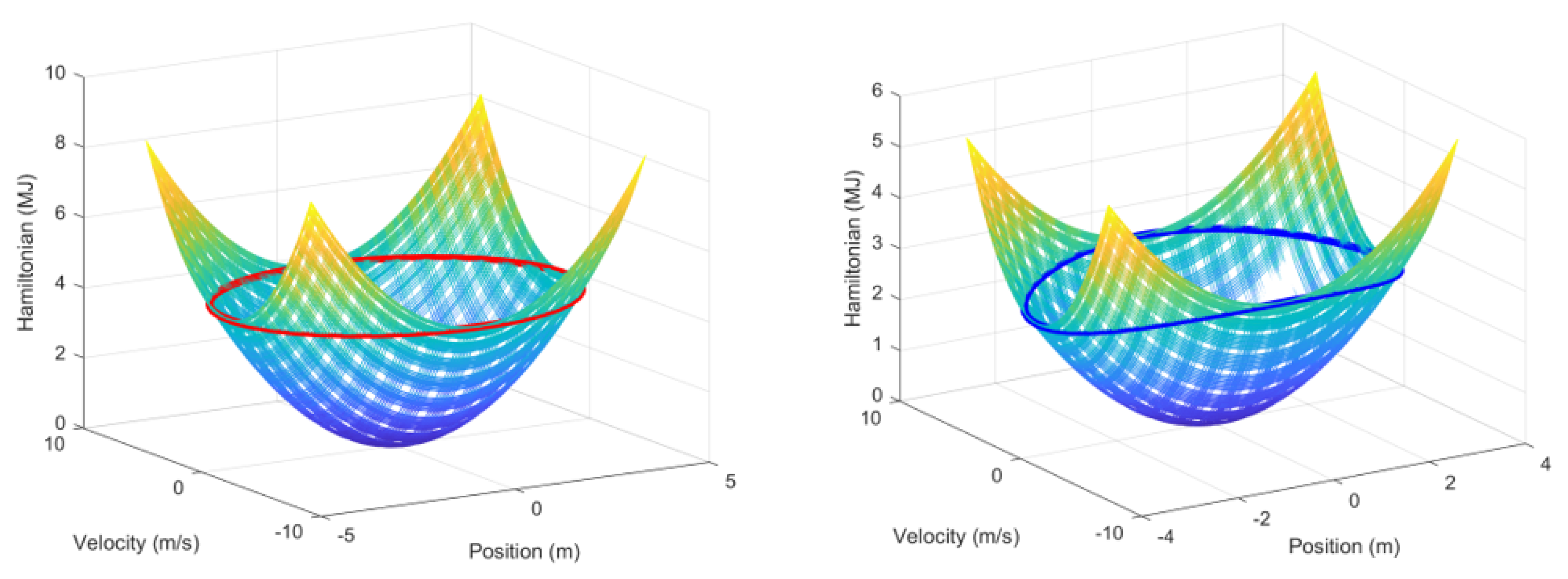
The optimal power/energy capture for an unconstrained linear WEC is a linear limit cycle (constant energy orbit across the Hamiltonian surface) which is also known as a second-order center. The optimal linear limit cycle, as well as non-optimal limit cycles for non-resonating circuits and power engineering applications, are discussed in [20,28]. The optimal and non-optimal limit cycles for the RCC WEC (Figure 1) are shown in Figure 4 along with the corresponding limit cycle comparisons shown in Figure 5, respectively. For the purposes of this discussion, a linear RCC WEC equation of motion for a single sinusoidal frequency can be stated as

$$m\ddot{z}+kz=-c\dot{z}+F_{0}cos\mathsf{\Omega }t+F_u,$$

(12)

where z and $\dot{z}$ are the heave displacement and velocity, respectively. The natural frequency of the system is $\omega =\sqrt{k/m}$. For the condition $\mathsf{\Omega }\equiv \omega$ the system will resonate.

The off-resonant case is equivalent to a parameter mis-match which could represent differing material properties or unaccounted mass properties. A simple change of a 15% offset in stiffness or $\tilde{\omega }=\sqrt{\tilde{k}/m}$ with $\tilde{k}=0.85k$ is shown in the corresponding plots (Figure 5) for the off-resonance condition. This results in a reduction in heave displacement and heave velocity. As an example, assume a simple rate feedback controller, $F_u=-R_{opt}\dot{z}$ then for the off-resonance versus resonance case the real power, $P_{real}=F_u\dot{z}$ will have a reduction in power/energy capture. The harvested energy is given as the integral of real power. The reactive power is defined as $P_{reac}=F_{reac}\dot{z}$.

4. Nonlinear Feedback Linearization and PDC3

A straightforward way to apply CCC to a nonlinear WEC is to apply feedback linearization [29]. A nonlinear WEC controller is designed by applying nonlinear feedback linearization to eliminate the nonlinear terms followed by applying PDC3 to the remaining linear system. A typical nonlinear WEC model for a regular wave could include nonlinear damping (Coulomb friction [29], Chapter 4 and typical square law drag [29], Chapter 1) and nonlinear stiffness (Duffing oscillator, hardening spring [29], Chapter 1) resulting in

$$M\ddot{z}+Kz+K_{NL}{z}^3=-c\dot{z}-c_{N{L}_1}sign\left(\dot{z}\right)-c_{N{L}_2}\dot{z}\left|\dot{z}\right|+F_{0}cos\mathsf{\Omega }t+F_u.$$

(13)

A nonlinear feedback controller can be implemented as

$$F_u=F_{u_{NL}}+F_{u_{PDC3}},$$

(14)

where

$$F_{u_{NL}}={\widehat{c}}_{N{L}_1}sign\left(\dot{z}\right)+{\widehat{c}}_{N{L}_2}\dot{z}\left|\dot{z}\right|+{\widehat{K}}_{NL}{z}^3,$$

(15)

and $F_{u_{PDC3}}$ is a PDC3 linear feedback controller (see Equation (2)). After applying the nonlinear feedback controller with perfect parameter cancellation or ${\widehat{c}}_{N{L}_1}=c_{N{L}_1}, {\widehat{c}}_{N{L}_2}=c_{N{L}_2}$, and ${\widehat{K}}_{NL}=K_{NL}$ and perfect sensor measurements the remaining system is a linear WEC for a regular wave or

$$M\ddot{z}+Kz=-c\dot{z}+F_{0}cos\mathsf{\Omega }t+F_{u_{PDC3}}.$$

(16)

This controller can be easily extended to irregular waves. The performance results of this nonlinear controller are given for an electrical system in [20,28]. A special case of nonlinear control that utilizes cubic spring feedback only is developed for a WEC and compared with PDC3 in [30]. The issues with the nonlinear feedback linearization controller are the required reactive power and the associated energy storage system as well as the power being consumed by the cancellation of the nonlinear terms. In the next section, the cubic spring controller is realized as a nonlinear geometric buoy to eliminate the issues of reactive power, energy storage, and nonlinear feedback linearization.

5. HSSPFC and Nonlinear Limit Cycles

HSSPFC can be applied to nonlinear WECs to design nonlinear resonators which take advantage of the nonlinear dynamics instead of eliminating them [30]. References [20,22] describe the process to extend the concepts of linear limit cycles to nonlinear limit cycle design. In particular, the goal of this section is to maximize the power/energy capture of the nonlinear WEC by properly shaping the buoy to produce reactive power from the water and generating super- and sub-harmonics that resonate at the desired wave frequencies.

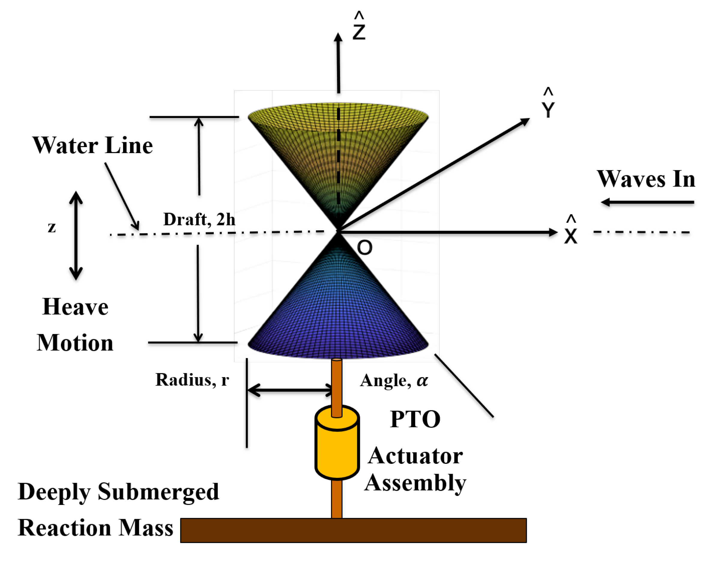
5.1. Hour-Glass (HG) WEC Design Model Development

A cubic hardening spring discussed in the previous section can be created by shaping the buoy into an hour-glass (HG) geometry as shown in Figure 6. The corresponding buoy geometric parameters for both the HG and RCC designs are given in

Table 1. Hour-glass (HG) and RCC buoy geometric parameters.

Parameter	Symbol	HG Range	RCC Value	Unit
Radius	r	5.72–10.0	4.47	m
Height	h	8.18–2.68	4.47	m
Angle	$\alpha$	50–70	0.00	deg

, respectively.

The HG and RCC (dashed line) cross-sections are presented in Figure 7 and will be modeled using a small body approximation [16,31]. Note, the volume of the HG and RCC are constrained to be equal.

The hydrostatic force is caused by the submerged volume of the HG. The volume of one cone is

$$V_{cone}=\frac{1}{3}\pi r^{2}h=\frac{1}{3}\pi {\overline{\alpha }}^2{h}^3$$

(17)

for

$$r=htan\alpha =h\overline{\alpha }.$$

(18)

Assuming the neutral buoyancy line is located at the apex of the cones, the volume as a function of position of the center of volume is

$$V\left(z\right)=\frac{1}{3}\pi {\overline{\alpha }}^2{h}^3-\frac{1}{3}\pi {\overline{\alpha }}^2{z}^3=\frac{1}{3}\pi {\overline{\alpha }}^2\left[h^3-z^3\right].$$

(19)

The hydrostatic force for the buoy staying in the water is

$$F_h=F_g+F_{buoy}=-mg+\rho gV\left(z\right)=-\frac{1}{3}\pi \rho g{\overline{\alpha }}^2{z}^3.$$

(20)

The potential function for this hydrostatic force is

$${\mathcal{V}}_{buoy}=\frac{1}{12}\pi \rho g{\overline{\alpha }}^2{z}^4.$$

(21)

The nonlinear WEC model for the HG is developed from [16,31] where the excitation force in heave is dominated by the hydrostatic component

$$F_{ex}\approx \rho g{S}_{w}A.$$

(22)

This is essentially the hydrostatic force. The non-uniform water plane area, $S_w$, for the cone is

$$S_w\left(\zeta \right)=\pi r{\left(z\right)}^2=\pi {\overline{\alpha }}^2{\left[z-\zeta \right]}^2,$$

(23)

where $\zeta$ is the vertical position of the center of volume of HG (see Figure 7). The hydrostatic force is proportional to the submerged volume of the body, and for very long waves, the wave profile can be considered as having the same value of the vertical coordinate across the cone (see Figure 7). That is, $z\approx \eta$ and where $\eta$ is the wave elevation. The submerged volume is

$$\begin{array}{cc}\hfill V_{sub}& =V_{cone}+{\int }_{\zeta }^{\eta }\pi {\overline{\alpha }}^2{(z-\zeta )}^{2}dz\hfill \\ \hfill & =V_{cone}+{\int }_{\zeta }^{\eta }\pi {\overline{\alpha }}^2(z^2-2\zeta z+{\zeta }^2)dz\hfill \\ \hfill & =V_{cone}+\pi {\overline{\alpha }}^2\left[\frac{1}{3}{\eta }^3-\zeta {\eta }^2+{\zeta }^2\eta -\frac{1}{3}{\zeta }^3\right].\hfill \end{array}$$

(24)

Assuming the added mass and radiation damping are constant with frequency [19,21] then

$$m\ddot{\zeta }=-b\dot{\zeta }-mg+\rho g{V}_{sub}+F_u.$$

(25)

Upon substitution of $V_{sub}$ from Equation (24) gives the equation of motion as

$$m\ddot{\zeta }+b\dot{\zeta }+\rho g\pi {\overline{\alpha }}^2\left[\frac{1}{3}{\zeta }^3-\eta {\zeta }^2+{\eta }^2\zeta \right]=\frac{\rho g\pi {\overline{\alpha }}^2}{3}{\eta }^3+F_u,$$

(26)

which contains the cubic hardening spring with $F_u=-R_{opt}\dot{\zeta }$. The Hamiltonian for the HG WEC is

$${\mathcal{H}}_{buoy}={\mathcal{T}}_{buoy}+{\mathcal{V}}_{buoy}=\frac{1}{2}m{\dot{\zeta }}^2+\frac{1}{12}\pi \rho g{\overline{\alpha }}^2{\zeta }^4,$$

(27)

where ${\mathcal{T}}_{buoy}$ and ${\mathcal{V}}_{buoy}$ are the kinetic and potential energies of the buoy, respectively. To fully understand the value of the HG WEC design, a RCC WEC design with nonlinear feedback control will be developed in the next section. The simulation results and comparisons for the HG and RCC models and controllers will be presented in Section 6.

5.2. RCC WEC Design Model Development

For the RCC buoy the hydrostatic force is caused by the submerged volume of the RCC (see Figure 7). The volume of one-half the RCC buoy is

$$V_{RCC}=\frac{1}{2}{r}^{2}h.$$

(28)

The volume as a function of position of the center of volume is

$$V=V\left(z\right)=V_{RCC}+{\int }_{\zeta }^{\eta }\pi r^{2}dz=V_{RCC}+\pi r^2(\eta -\zeta ).$$

(29)

The equation of motion becomes

$$m\ddot{\zeta }=-b\dot{\zeta }-mg+\rho gV+F_u.$$

(30)

Substitute Equation (29) into Equation (30) yields

$$m\ddot{\zeta }=-b\dot{\zeta }-mg+\rho g{V}_{RCC}+\pi r^2(\eta -\zeta )+F_u.$$

(31)

The equilibrium position is

$$mg=\rho g{V}_{RCC},$$

(32)

which then yields after simplification

$$m\ddot{\zeta }+b\dot{\zeta }+\rho g\pi r^2\zeta =\rho g\pi r^2\eta +F_u.$$

(33)

Note that $\zeta$ is the vertical position of the center of the RCC buoy geometry and $\eta$ is the wave elevation or driving input to the system (see Figure 7) for either regular or irregular waves.

An additional nonlinear (NL) restoring force can be introduced to the equation of motion (Equation (33)) as

$$m\ddot{\zeta }+b\dot{\zeta }+k_{LIN2}\zeta =F_{ex}+F_u+F_{NL},$$

(34)

where $k_{LIN2}=\rho g\pi r^2$ and the external wave force input is $F_{ex}=k_{LIN2}\eta$. For the purposes of this study a nonlinear restoring force can be introduced as a regulatory cubic spring along with resistive damping (rate feedback) control or

$$\begin{array}{cc}\hfill F_{NL}& =-k_{NL2}{\zeta }^3\hfill \end{array}$$

(35)

$$\begin{array}{cc}\hfill F_u& =-R_{opt}\dot{\zeta }.\hfill \end{array}$$

(36)

The Hamiltonian for the RCC WEC design is

$${\mathcal{H}}_{buoy}={\mathcal{T}}_{buoy}+{\mathcal{V}}_{buoy}=\frac{1}{2}m{\dot{\zeta }}^2+\frac{1}{4}{k}_{NL2}{\zeta }^4.$$

(37)

This RCC WEC design dynamic model and control version will be utilized to contrast and compare with the HG WEC design discussed in Section 5.1.

The final RCC WEC design modification explores a nonlinear feedback control with position error and rate feedback defined as

$$\begin{array}{cc}\hfill F_{NL}& =0\hfill \end{array}$$

(38)

$$\begin{array}{cc}\hfill F_u& =k_{NL2}{(\widehat{\eta }-\widehat{\zeta })}^3-R_{opt}\dot{\widehat{\zeta }}.\hfill \end{array}$$

(39)

When the cubic term is expanded to

$$F_u=k_{NL2}({\widehat{\eta }}^3-3{\widehat{\eta }}^2\widehat{\zeta }+3\widehat{\eta }{\widehat{\zeta }}^2-{\widehat{\zeta }}^3)-R_{opt}\dot{\widehat{\zeta }}$$

(40)

demonstrates that the individual terms compare similar to the HG WEC design interaction with the waves (see Equation (26)).

This nonlinear feedback strategy focuses on nonlinear oscillations to multiply and/or magnify the energy and power capture from the WEC device. By introducing a cubic spring in the feedback loop a significant increase in power capture results. This can be realized as a mechanical nonlinear spring in combination with an energy storage device to help transmit reactive power between cycles or geometric modifications. Alternatively, the cubic hardening spring can be realized by shaping the buoy to produce reactive power from the waves.

In contrast to the HG WEC design with resistive damping feedback, the RCC WEC design with nonlinear feedback control, the following exceptions are required; (i) estimated wave elevation $\widehat{\eta }$ and (ii) measured vertical buoy position $\widehat{\zeta }$. The elegance of the HG WEC design is that the reactive power and energy storage system requirements are inherently embedded in the nonlinear buoy geometry which only requires simple rate feedback control. In addition, the estimated wave elevation and vertical buoy position are intrinsic to the HG WEC design.

6. Case Study Simulation Results

In this section, the case studies and simulation results are discussed for; (i) nonlinear resonator, (ii) single frequency inputs, and (iii) multi-frequency spectrum inputs. A simplified optimal HG WEC design (optimize $\alpha$ subject to volumetric constraints leading to draft limits) is contrasted with an RCC WEC design, respectively. A volume constraint on displaced fluid was imposed on both the RCC and HG WECs to be equivalent or

$$V_{HG}=V_{RCC}.$$

(41)

The position constraints for the RCC and the HG WECs resulted in draft limits shown in

Table 2. Single frequency numerical results.

Parameter	Unit	RCCNL	RCC	HG	RCC10	HG10	RCC20	HG20	RCC30	HG30
$\alpha$	deg	N/A	N/A	59.5	N/A	56.5	N/A	53.5	N/A	50.9
${\overline{R}}_{opt}$	$\left(\mathrm{N}\frac{\mathrm{s}}{\mathrm{m}}\right)·{10}^5$	3.844	4.456	N/A	4.848	N/A	5.242	N/A	5.746	N/A
$h_{limit}$	m	4.47	4.47	4.53	4.47	4.896	4.47	5.274	4.47	5.614
$E_{max}$	MJ	129	146	146	160	171	173	197	183	226

. The simplified optimization, used for the Bretschneider spectrum, for the HG WEC is a function of $\alpha$ which constrains the heave motion and the wave height. Note that $\alpha$ will be sea state-dependent and would be adapted to meet each specific condition for the actual application. The buoy [14] effective mass is $m=1.76\times {10}^5$ kg, linear damping coefficient is $b=170$ N s/m, and linear stiffness coefficient is $k=4.544915\times {10}^5$ kg/${\mathrm{s}}^2$. The nonlinear stiffness coefficient used for the $RC{C}_{NL}$ case is $K_{NL}=1.4141\times {10}^4$ N/${\mathrm{m}}^3$. Note the damping and nonlinear stiffness for the $RC{C}_{NL}$ buoy are from reference [30]. To constrain the maximum displacement for the RCC buoy, the linear damping coefficients were increased as given in Table 2. This prevents the RCC buoy from coming out of the water or totally submerging causing over-topping.

6.1. Nonlinear Resonator Results

The goal of this section is to show the design characteristics that started from a simple RCC with nonlinear control design (utilizing a cubic spring [30]), that was initially employed to evaluate a NL geometric shape, resulted in the HG WEC design. The nonlinear limit cycles constrained to the Hamiltonian surface, for the HG WEC design as compared to the RCC NL cubic spring WEC design and are shown in Figure 8. The corresponding nonlinear limit cycle comparisons are shown in Figure 9, respectively.

The differences in the shapes and responses can be traced back to the comparison of Equations (26), (34) and (40), respectively. Initially, the HG WEC design includes the cubic expansion and interaction between the device and the fluid media whereas the initial RCC WEC design does not. However, the key highlight—a nonlinear control design was employed to design a nonlinear geometric HG WEC with the desired effects and characteristics associated with providing reactive power that is intrinsic to the design.

6.2. Single Frequency Results

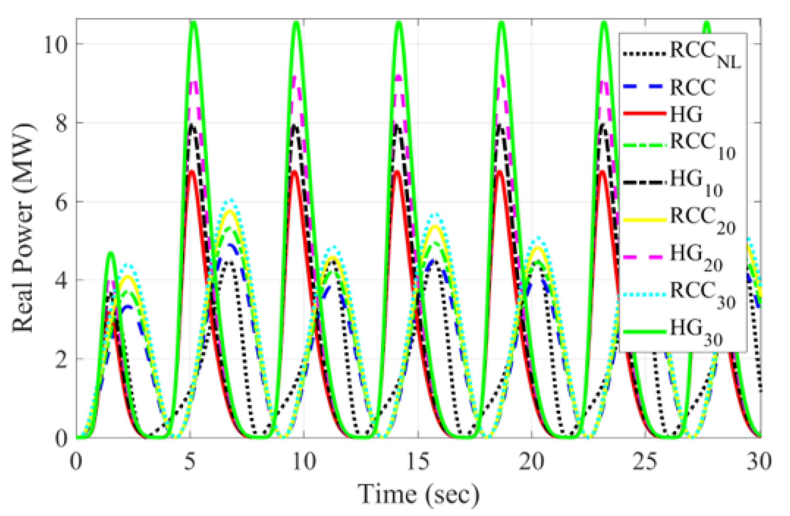
Numerical simulation results are presented for each of the variations considered. The RCC WEC design included both a PDC3 ($RCC$) and nonlinear cubic spring ($RC{C}_{NL}$) controllers. Initially, the HG WEC design ($HG$) used an $\alpha$ value to match the corresponding PDC3 RCC WEC design. These three designs are considered as the baseline designs during the numerical simulation results. Note that the full draft potential for the HG WEC design was investigated by comparing the HG and RCC WEC designs for incrementally increasing wave heights (10%, 20%, 30%). These are also noted as subscripts in the numerical results ($RC{C}_{10}, H{G}_{10}, RC{C}_{20}, H{G}_{20}, RC{C}_{30}, H{G}_{30}$). All results were performed over a 100 s time window. A 0.111 Hz single frequency wave input was employed for all cases. The first 30 s of the 100 s duration are shown in Figure 10.

The harvested energy for all buoy designs is shown in Table 2 and Figure 11, respectively. Table 2 includes; (1) $\alpha$, steepness angle limit, (2) ${\overline{R}}_{opt}$, effective optimal damping for the RCC buoys, (3) $h_{limit}$ draft for all buoys, and (4) $E_{max}$, the maximum harvested energy, for the 100 s duration, used as a metric of performance for all buoy designs. The harvested energy was determined between 30 and 100 s to avoid initial transients, such that all buoys are in steady state operation. Overall the HG buoy designs resulted in increased harvested energy; 6.9%, 13.9%, and 23.5%, for increased waves; 10%, 20%, 30%, in comparison to the RCC buoy designs, respectively.

The external forces and control forces for all cases are shown in Figure 12 and Figure 13, respectively. Note that after an initial 10 s period the transient responses converges to steady-state operation.

The RCC with PDC3 reactive power responses are symmetric and cancel point-by-point [20,22] (linear) at resonance. For the more general solution the point-by-point force balance is replaced by a cyclic balance between the power flowing into the system versus the power being dissipated within the system (or equal area under the reactive power curve) or

$${\mathcal{H}}_{cyclic}={\oint }_{\tau }\dot{\mathcal{H}}dt=0,$$

(42)

where $\tau$ is over the cycle time. For the nonlinear responses, the RCC with nonlinear feedback and the HG will have equal areas over the respective cycles. The reactive power for all cases is shown in Figure 14.

The real power for all cases is shown in Figure 15. Note that for increasing wave input, the HG buoys increase in real power production at a higher rate than the equivalent RCC buoy designs.

The corresponding buoy position and velocity responses for all cases are shown in Figure 16 and Figure 17, respectively. Each buoy design position response observes the $h_{limit}$ parameter given in Table 2. For increasing wave inputs, the corresponding velocity responses also increase, resulting in higher speeds and real power production (primarily for the HG buoy).

6.3. Bretschneider Multi-Spectrum Results

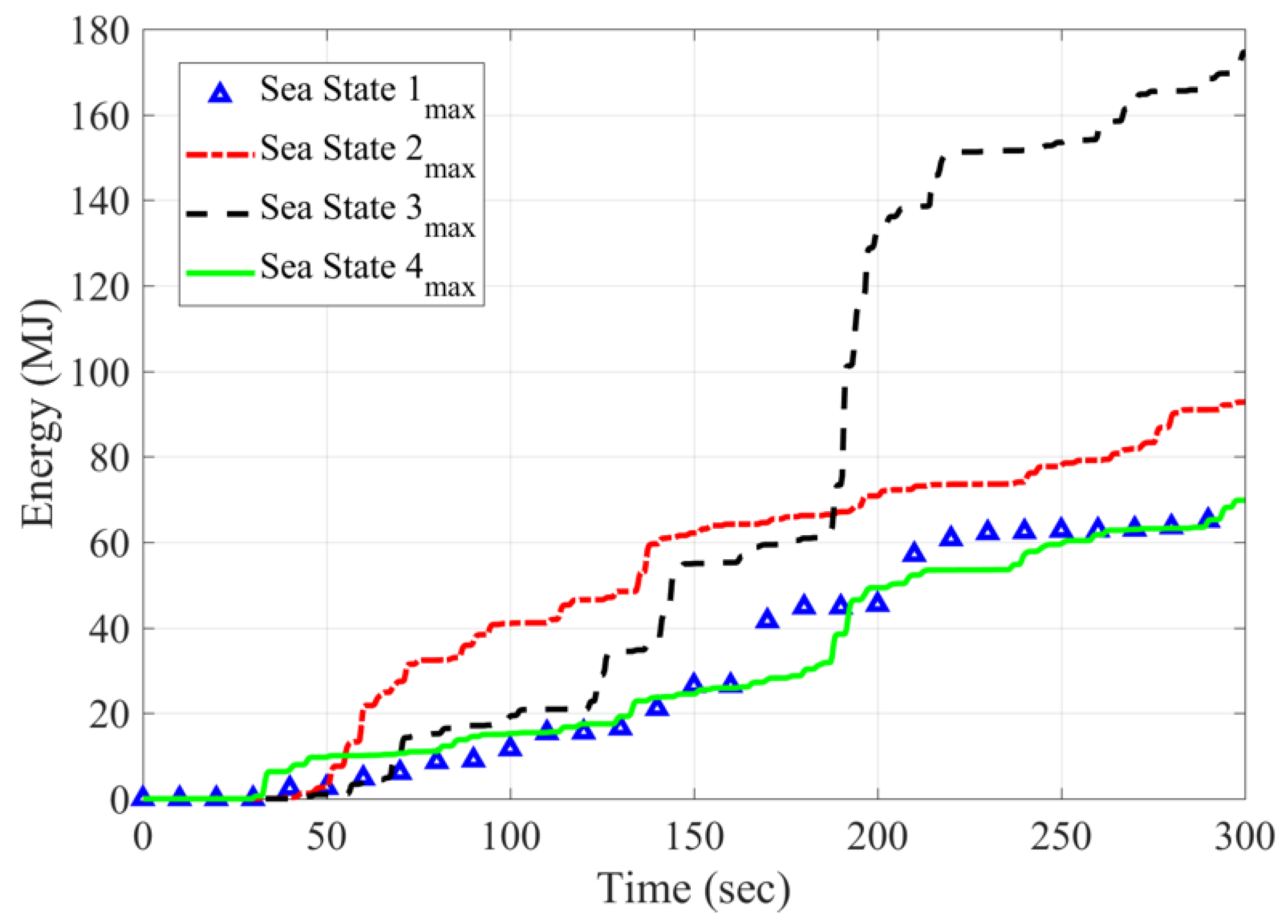
A Bretschneider multi-spectrum containing multi-frequency content includes four varying sea states with five minute durations. These were generated for the HG buoy design to fully evaluate the power/energy capture extraction. These varying sea states were derived based on actual buoy data from Nags Head, NC with a scale factor of 3 applied to boost the wave height $H_s$ to provide sufficient amplification for the HG buoy to be evaluated. The spectrum was generated with the Bretschneider and corresponding time domain data by spec2dat Matlab functions from the toolbox in [32]. The varying sea state parameters are given in

Table 3. Sea state parameters.

Sea State	${\mathit{H}}_{\mathit{s}}$ (m)	${\mathit{T}}_{\mathit{p}}$ (sec)	Duration (sec)
1	5.7	8.0	300.0
2	6.6	6.6	300.0
3	7.8	7.8	300.0
4	6.9	11.0	300.0

with the corresponding Bretschneider spectrum in the frequency domain shown in Figure 18.

The HG design was evaluated with a volumetric constraint given by Equation (41). The steepness angle, $\alpha$, shown in Figure 6, was swept from 55–75 degrees to define the design space for each varying sea state. The energy captured at the end of the 5 min duration was recorded and the results are given in

Table 4. HG buoy Bretschneider spectrum sea state results.

Angle	Draft	Sea State 1	Sea State 2	Sea State 3	Sea State 4
$\mathbf{\alpha }$	hhalf	Emax	Emax	Emax	Emax
deg	m	MJ	MJ	MJ	MJ
55	5.084	26.485	23.935	174.63	32.230
60	4.470	43.240	39.235	SAT	48.564
65	3.8767	67.170	61.550	–	69.790
70	3.2864	SAT	92.752	–	SAT
75	2.680	–	SAT	–	–

Note: for all Sea States ${\overline{R}}_{opt} = 4.4044\left(\mathrm{N}\frac{\mathrm{s}}{\mathrm{m}}\right)·{10}^5$.

.

A SAT (saturation) recorded in the table column indicates the HG buoy for the corresponding $\alpha$ angle saturated the geometric upper/lower vertical displacement limits and the previous angle is considered the maximum energy capture result. Saturation indicates that the HG buoy is either completely out of the water or totally submerged/over-topping. The maximum energy captured for each sea state is plotted in Figure 19.

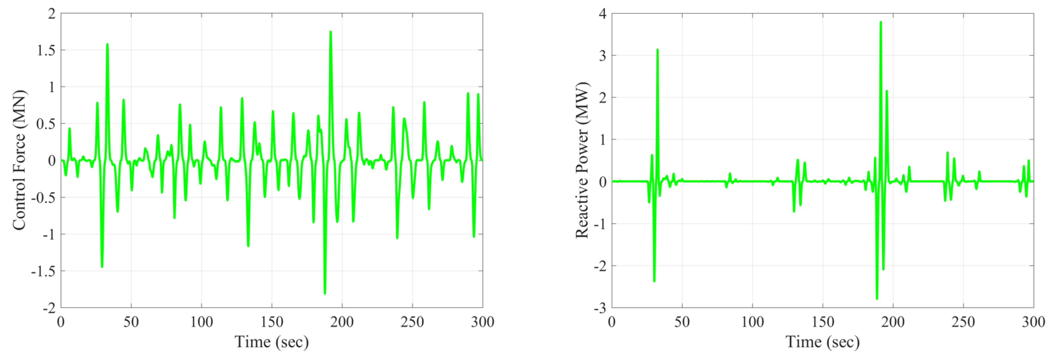
The complete time simulation results for sea state 4 ($SS4$) are shown in the following figures (color code noted as green in all plots). The corresponding Bretschneider wave input (left) and external force (right) are shown in Figure 20. The control force (left) and reactive power (right) are shown in Figure 21. Note that the reactive power is generated intrinsically by the NL HG buoy geometry. The real power (left) and harvested energy (right) are shown in Figure 22. Positive values represent power and harvested energy generated from the WEC devices. The final harvested energy value at the end of the 5 min duration (Figure 22 right) corresponds to the tabulated value 69.790 MJ in Table 4. The WEC buoy position (left) and velocity (right) are given in Figure 23. The trend shows for increased $\alpha$ the power and harvested energy increases. However, given the volume constraint on the HG WEC design, the draft decreases as $\alpha$ increases which constrains upper limit on the maximum power/energy capture since the motion of the HG WEC buoy is constrained. For these realistic wave forms, the HG WEC buoy shows desirable characteristics.

7. Conclusions

This paper extends the concept of CCC of linear WECs to NL WECs by designing optimal limit cycles with HSSPFC. It was shown that CCC for a regular wave is equivalent to a power factor of one in electrical power networks, equivalent to mechanical resonance in an MSD system, and equivalent to a linear limit cycle constrained to a Hamiltonian surface defined in HSSPFC. Specifically, the optimal linear limit cycle is defined as a second-order center in the phase plane projection of the constant energy orbit across the Hamiltonian surface. This concept of CCC described by a linear limit cycle constrained to a Hamiltonian surface was extended to NL limit cycles constrained to a Hamiltonian surface to maximize energy harvesting by the NL WEC design. Numerical simulations verified these cases. This current HG WEC design and case study show desirable characteristics; (1) no required reactive power or energy storage system due to the geometry buoy shape, (2) no cancellation of nonlinear terms that consume power, (3) the nonlinear resonator increases the capture width by including sub/super harmonics in the input waves, (4) by increasing the draft and speed of the HG buoy more energy is harvested, and (5) the NL WEC buoy shape creates equivalent wave height and buoy motion measurements that are naturally incorporated. Future work will include a refined optimization of the HG WEC design with respect to varying and site-dependent sea state conditions.

References

- Li, G.; Weiss, G.; Mueller, M.; Townley, S.; Belmont, M.R. Wave energy converter control by wave prediction and dynamic programming. Renew. Energy 2012, 48, 392–403. [Google Scholar] [CrossRef] [Green Version]
- Falnes, J. A review of wave-energy extraction. Mar. Struct. 2007, 20, 185–201. [Google Scholar] [CrossRef]
- Ringwood, J.; Bacelli, G.; Fusco, F. Energy-Maximizing Control of Wave-Energy Converters: The Development of Control System Technology to Optimize Their Operation. IEEE Control Syst. Mag. 2014, 34, 30–55. [Google Scholar] [CrossRef]
- Hals, J.; Falnes, J.; Moan, T. A Comparison of Selected Strategies for Adaptive Control of Wave Energy Converters. J. Offshore Mech. Arct. Eng. 2011, 133. [Google Scholar] [CrossRef]
- Cretel, J.; Lightbody, G.; Thomas, G.; Lewis, A. Maximisation of Energy Capture by a Wave-Energy Point Absorber Using Model Predictive Control. In Proceedings of the 18th IFAC World Congress, Milano, Italy, 28 August–2 September 2011; Volume 44, pp. 3714–3721. [Google Scholar]
- Bacelli, G.; Ringwood, J.V.; Gilloteaux, J.C. A control system for a self-reacting point absorber wave energy converter subject to constraints. In Proceedings of the 18th IFAC World Congress, Milano, Italy, 28 August–2 September 2011; pp. 11387–11392. [Google Scholar]
- Abdelkhalik, O.; Robinett, R.; Bacelli, G.; Coe, R.; Bull, D.; Wilson, D.; Korde, U. Control Optimization of Wave Energy Converters Using a Shape-Based Approach. In ASME Power & Energy 2015; ASME: San Diego, CA, USA, 2015. [Google Scholar]
- Abdelkhalik, O.; Robinett, R.; Zou, S.; Bacelli, G.; Coe, R.; Bull, D.; Wilson, D.; Korde, U. On the control design of wave energy converters with wave prediction. J. Ocean Eng. Mar. Energy 2016, 2, 473–483. [Google Scholar] [CrossRef] [Green Version]
- Faedo, N.; Olaya, S.; Ringwood, J.V. Optimal control, MPC and MPC-like algorithms for wave energy systems: An overview. IFAC J. Syst. Control 2017, 1, 37–56. [Google Scholar] [CrossRef] [Green Version]
- Abraham, E. Optimal Control and Robust Estimation for Ocean Wave Energy Converters. Ph.D. Thesis, Department of Aeronautics, Imperial College London, London, UK, 2013. [Google Scholar]
- Retes, M.; Giorgi, G.; Ringwood, J. A Review of Non-Linear Approaches for Wave Energy Converter Modelling. In Proceedings of the 11th European Wave and Tidal Energy Conference, Nantes, France, 6–11 September 2015. [Google Scholar]
- Wolgamot, A.; Fitzgerald, C. Nonlinear Hydrodynamic and Real Fluid Effects on Wave Energy Converters. Proc. Inst. Mech. Eng. Part A J. Power Energy 2015, 229, 772–794. [Google Scholar] [CrossRef]
- Giorgi, G.; Retes, M.; Ringwood, J. Nonlinear Hydrodynamic Models for Heaving Buoy Wave Energy Converters. In Proceedings of the Asian Wave and Tidal Energy Conference (AWETEC 2016), Singapore, 24–28 October 2016. [Google Scholar]
- Abdelkhalik, O.; Darani, S. Optimization of nonlinear wave energy converters. Ocean Eng. 2018, 162, 187–195. [Google Scholar] [CrossRef]
- Darani, S.; Abdelkhalik, O.; Robinett, R.; Wilson, D. A hamiltonian surface-shaping approach for control system analysis and the design of nonlinear wave energy converters. J. Mar. Sci. Eng. 2019, 7, 48. [Google Scholar] [CrossRef] [Green Version]
- Falnes, J. Ocean Waves and Oscillating Systems, 1st ed.; Cambridge University Press: Cambridge, NY, USA, 2002. [Google Scholar]
- Song, J.; Abdelkhalik, O.; Robinett, R.; Bacelli, G.; Wilson, D.; Korde, U. Multi-Resonant Feedback Control of Heave Wave Energy Converters. Ocean Eng. 2016, 127, 269–278. [Google Scholar] [CrossRef]
- Abdelkhalik, O.; Zou, S.; Robinett, R.; Bacelli, G.; Wilson, D.; Coe, R.; Korde, U. Multi-Resonant Feedback Control of Three Degree-of-Freedom Wave Energy Converters. IEEE Trans. Sustain. Energy 2017, 8, 1518–1527. [Google Scholar] [CrossRef]
- Wilson, D.; Bacelli, G.; Coe, R.; Bull, D.; Abdelkhalik, O.; Korde, U.; Robinett, R. A Comparison of WEC Control Strategies; Sandia Report, URR, SAND2016-4293; Sandia National Laboratories: Albuquerque, NM, USA, 2016.
- Robinett, R.; Wilson, D. Nonlinear Power Flow Control Design: Utilizing Exergy, Entropy, Static and Dynamic Stability, and Lyapunov Analysis; Springer: London, UK, 2011. [Google Scholar]
- Wilson, D.; Bacelli, G.; Robinett, R.; Korde, U.; Abdelkhalik, O.; Glover, S. Order of Magnitude Power Increase from Multi-Resonance Wave Energy Converters. In Proceedings of the OCEANS 2017—Anchorage, Anchorage, AK, USA, 18–21 September 2017. [Google Scholar]
- Robinett, R.; Wilson, D. What is a Limit Cycle? Int. J. Control 2008, 81, 1886–1900. [Google Scholar] [CrossRef]
- Wikipedia. Limit Cycle. 2019. Available online: www.wikipedia.org (accessed on 27 January 2020).
- Ogata, K. Modern Control Engineering; Prentice-Hall, Inc.: Englewood Cliffs, NJ, USA, 1970. [Google Scholar]
- Smith, R. Circuits, Devices, and Systems: A First Course in Electrical Engineering, 3rd ed.; John Wiley & Sons: New York, NY, USA, 1976. [Google Scholar]
- Hartog, J.D. Mechanical Vibrations; McGraw-Hill: New York, NY, USA, 1934. [Google Scholar]
- Habiba, G.; Detroux, T.; Kerschen, G. Generalization of Den Hartog’s Equal-Peak Method for Nonlinear Primary Systems. In MATEC Web of Conferences, CSNDD 2014—International Conference on Structural Nonlinear Dynamics and Diagnosis; EDP Sciences: Les Ulis, France, 2014; Volume 16. [Google Scholar]
- Robinett, R.; Wilson, D. Nonlinear power flow control applied to power engineering. In Proceedings of the 2008 International Symposium on Power Electronics, Electrical Drives, Automation and Motion (SPEEDAM 2008), Ishchia, Italy, 11–13 June 2008. [Google Scholar]
- Slotine, J.J.; Li, W. Applied Nonlinear Control; Prentice-Hall, Inc.: Englewood Cliffs, NJ, USA, 1991. [Google Scholar]
- Wilson, D.; Robinett, R.; Abdelkhalik, O.; Bacelli, G. Nonlinear Control Design for Nonlinear Wave Energy Converters. In Proceedings of the John L. Junkins Dynamical Systems Symposium, College Station, TX, USA, 20–21 May 2018. [Google Scholar]
- Wilson, D.; Bacelli, G.; Weaver, W.; Robinett, R. 10x Power Capture Increased from Multi-Frequency Nonlinear Dynamics; Express LDRD Final Report, SAND2015-10446R; Sandia National Laboratories: Albuquerque, NW, USA, 2015.
- Perez, T.; Fossen, T. A Matlab Toolbox for Parametric Identification of Radiation-Force Models of Ships and Offshore Structures. Model. Identif. Control 2009, 30, 1–15. [Google Scholar] [CrossRef] [Green Version]
Figure 1.
Right circular cylinder (RCC) wave energy converter (WEC) buoy geometry.
Figure 2.
RLC electrical network schematic.
Figure 3.
Mass-spring-damper (MSD) mechanical system schematic.
Figure 4.
For a single frequency the resonance , (left) and off-resonance , (right) plots.
Figure 5.
For a single frequency the resonance and off-limit cycle comparisons, 3d (left) and phase-plane (right) plots.
Figure 6.
Hourglass nonlinear geometry WEC design.
Figure 7.
WEC HG and RCC buoy geometry 2D cross-sectional schematic.
Figure 8.
For a single frequency utilizes RCC with nonlinear (NL) cubic spring (left) and NL HG (right), respectively.
Figure 9.
NL limit cycle comparisons, 3d (left) and phase-plane (right), respectively.
Figure 10.
External wave input for the first 30 of 100 s duration.
Figure 11.
Harvested energy for all cases.
Figure 12.
External wave forces for the first 30 s of 100 s duration for all cases, respectively.
Figure 13.
Control forces for the first 30 s of 100 s duration for all cases, respectively.
Figure 14.
Reactive powers for the first 30 s of 100 s duration for all cases, respectively.
Figure 15.
Real powers for the first 30 s of 100 s duration for all cases, respectively.
Figure 16.
Buoy positions for the first 30 s of 100 s duration for all cases, respectively.
Figure 17.
Buoy velocities for the first 30 s of 100 s duration for all cases, respectively.
Figure 18.
Bretschneider spectral density for all sea states.
Figure 19.
Harvested energy for all varying sea states.
Figure 20.
SS4 external Bretschneider wave input (left) and external wave force (right), respectively.
Figure 21.
SS4 control force (left) and reactive power (right), respectively.
Figure 22.
SS4 real power (left) and harvested energy (right), respectively.
Figure 23.
SS4 position (left) and velocity (right), respectively.