Inter-Annual Variability of the Seawater Light Absorption in Surface Layer of the Northeastern Black Sea in Connection with Hydrometeorological Factors


Abstract
:1. Introduction
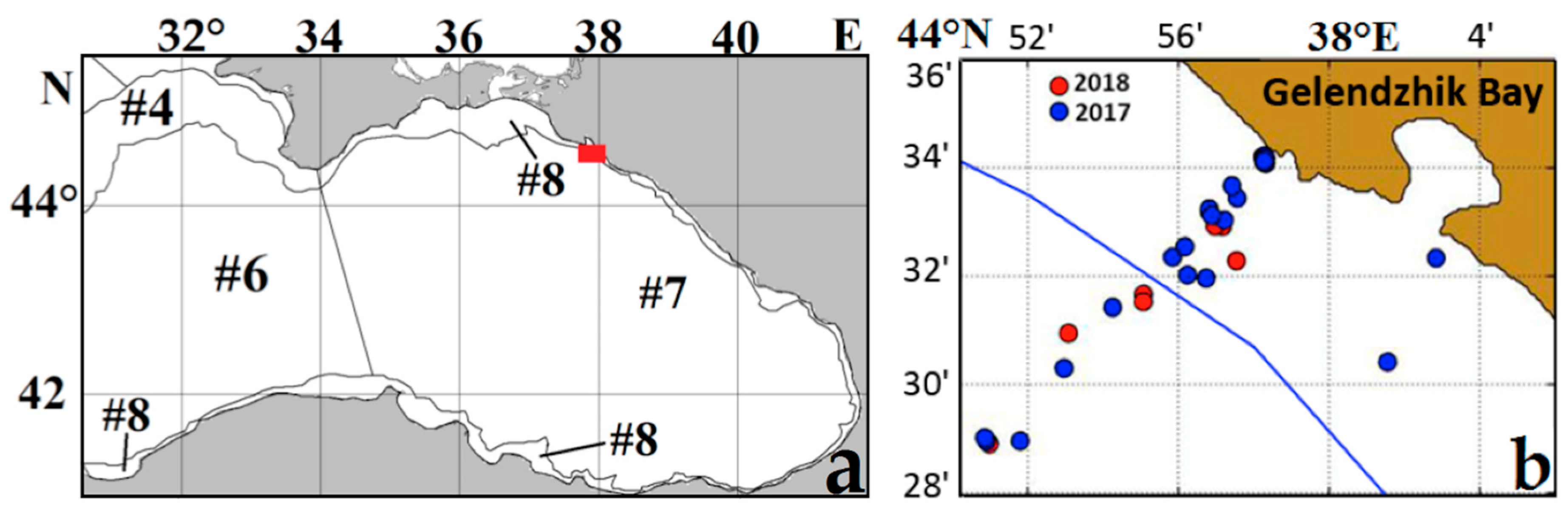
2. Materials and Methods
2.1. In Situ Studies
2.1.1. Measurements of the Spectral Absorption Parameters
2.1.2. Measurements of the Vertical Structure
2.2. Calculation of Hydrometeorological Parameters
2.3. Satellite Observation Data
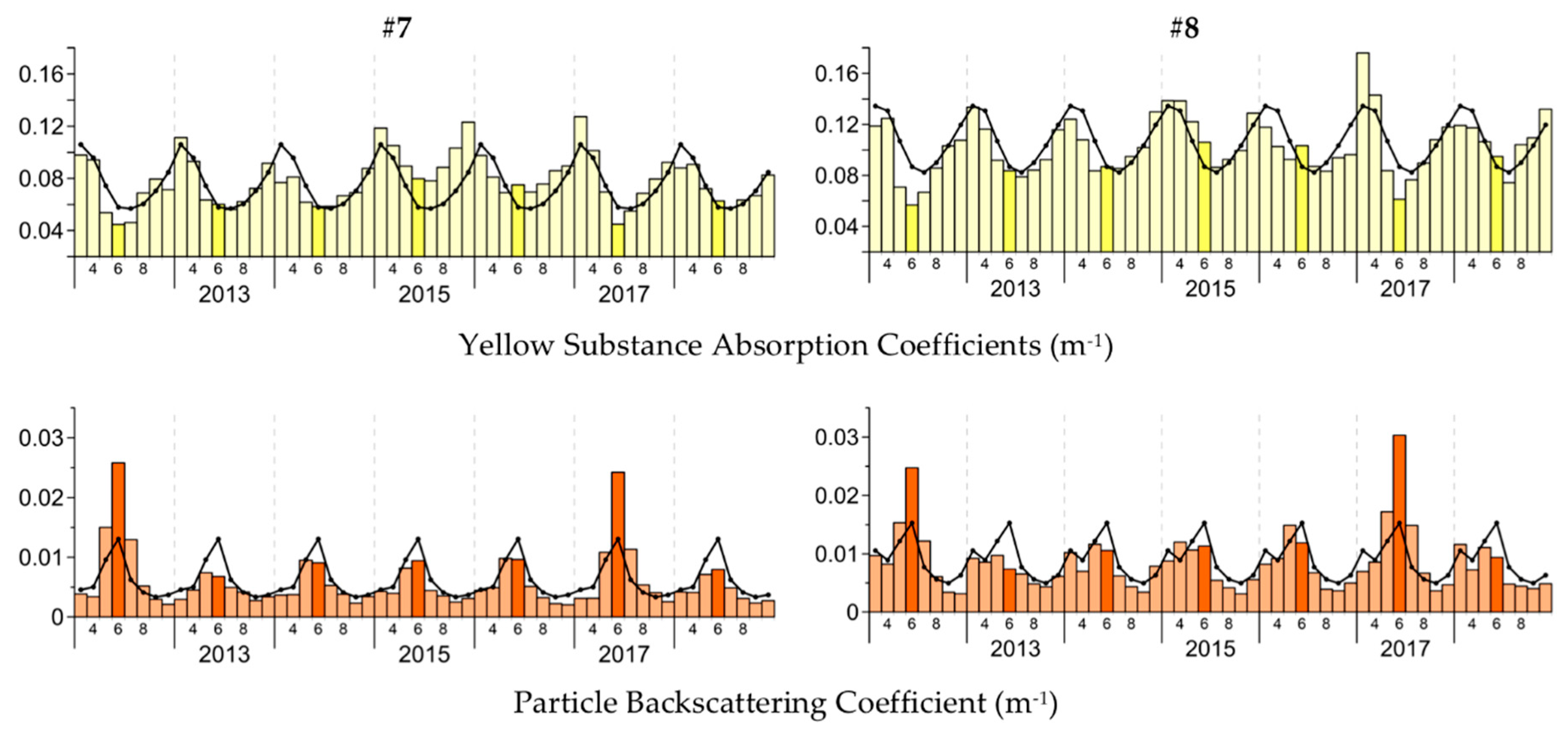
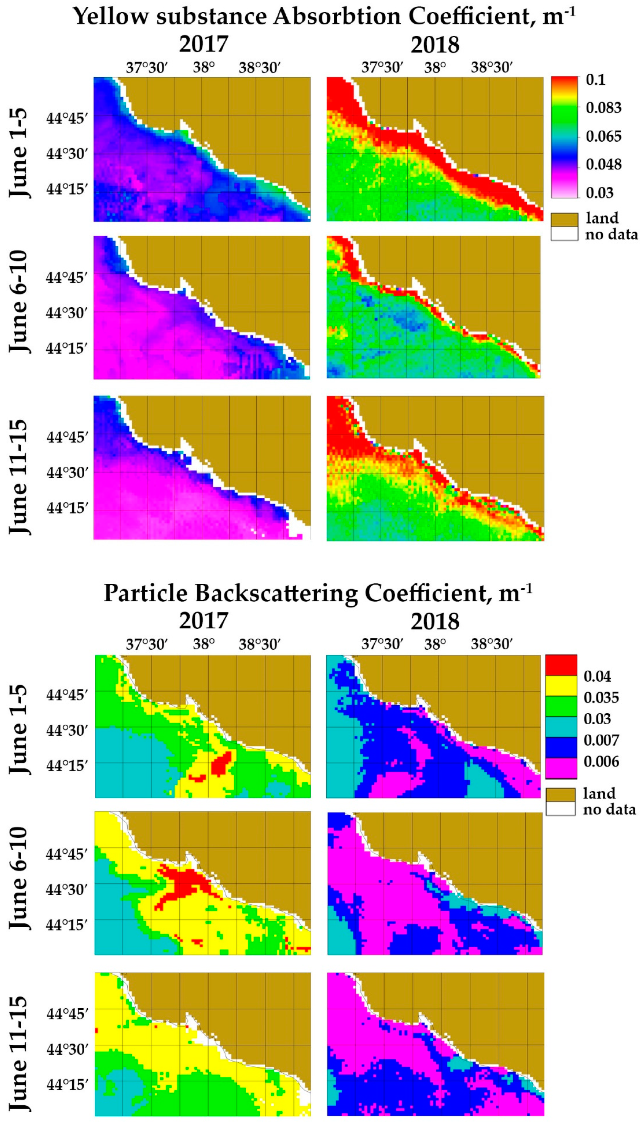
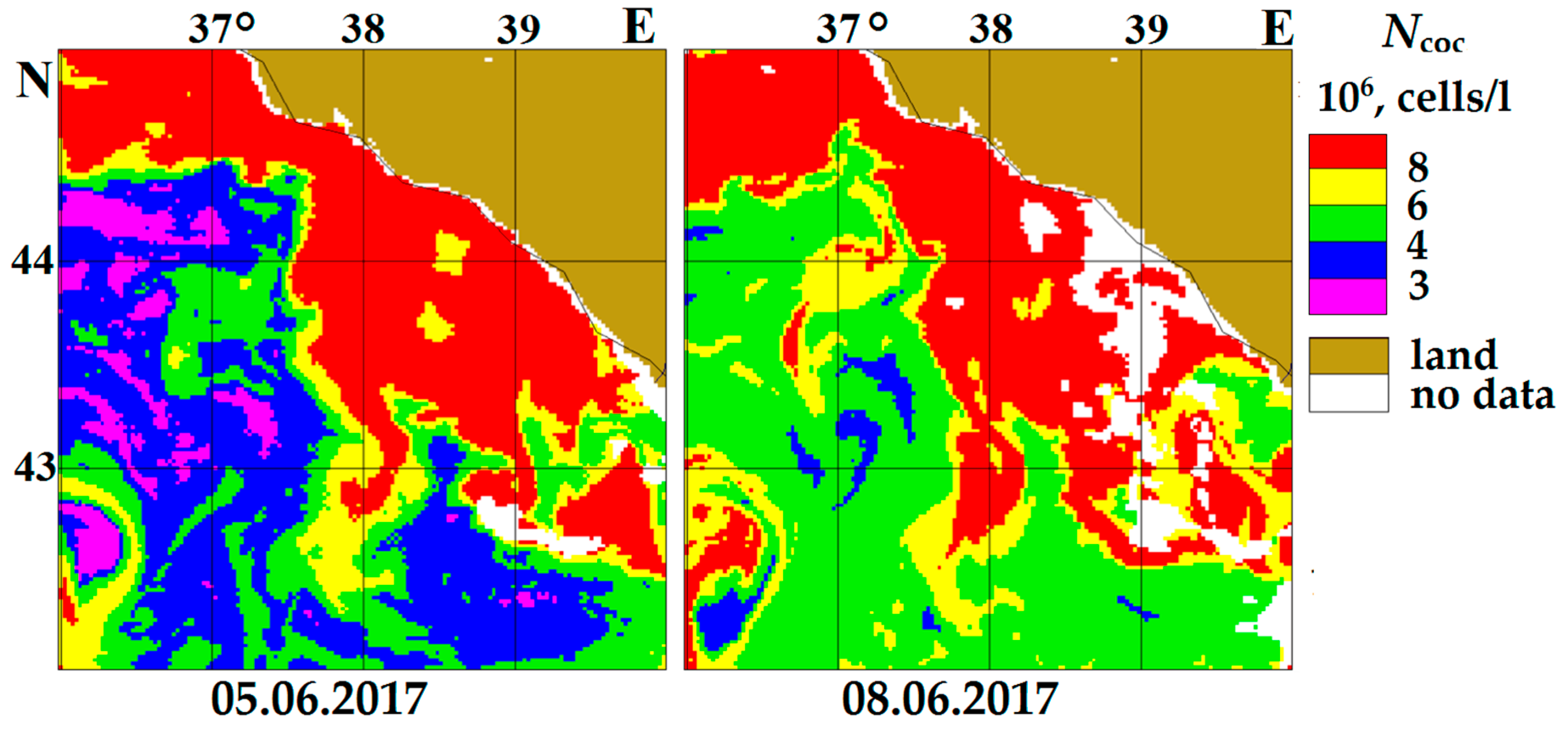
3. Results
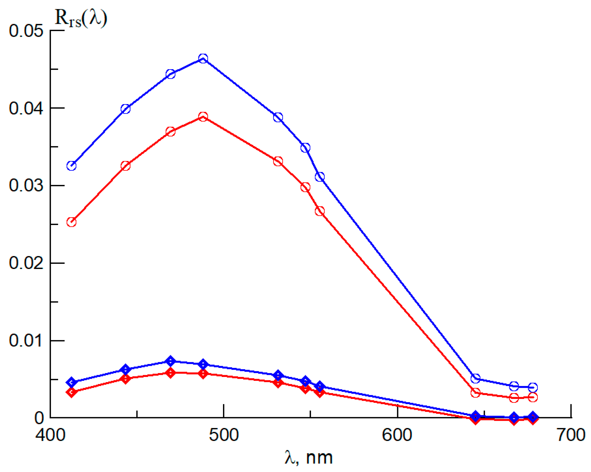
3.1. Satellite Data
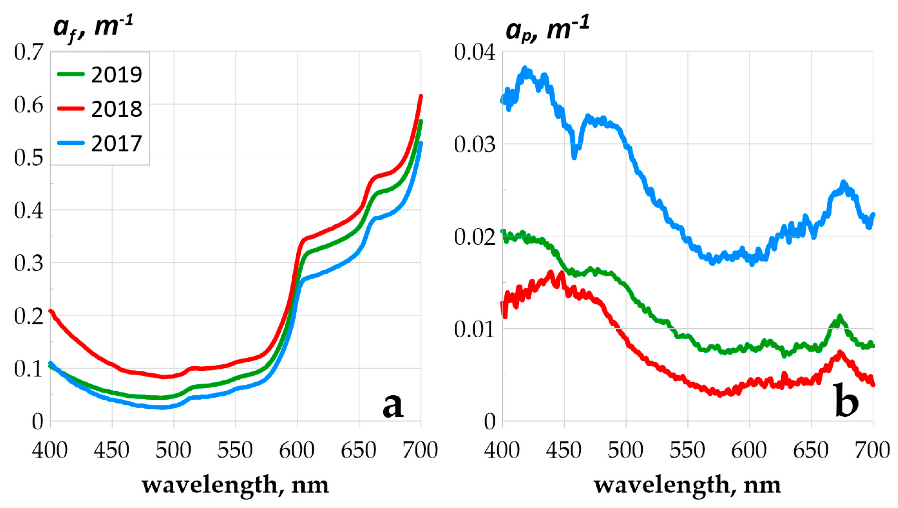
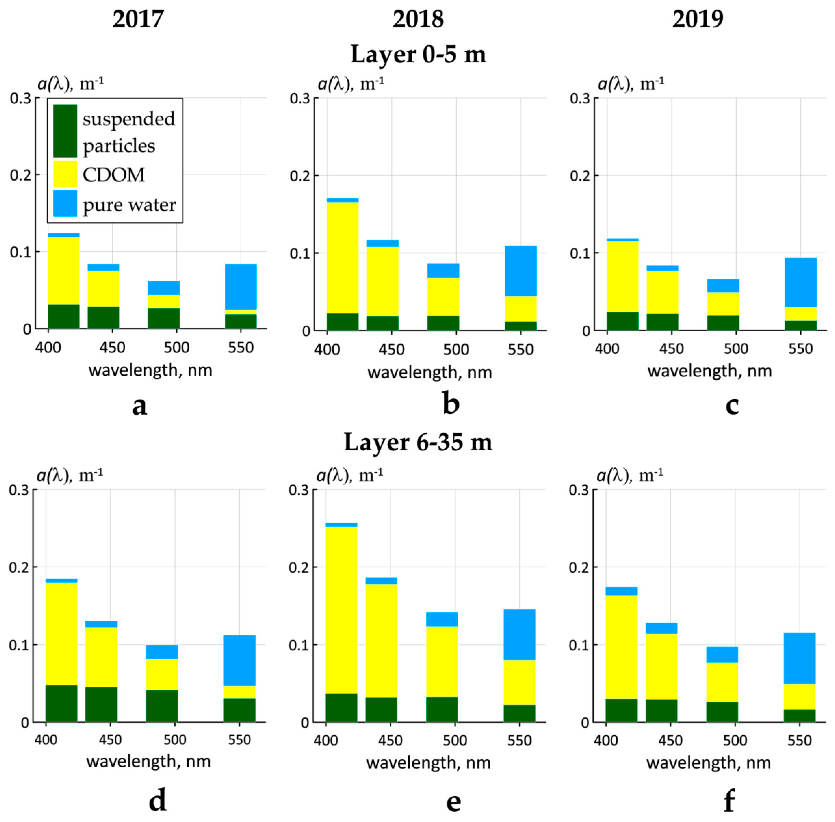
3.2. Spectral Absorption Measurements on the ICAM
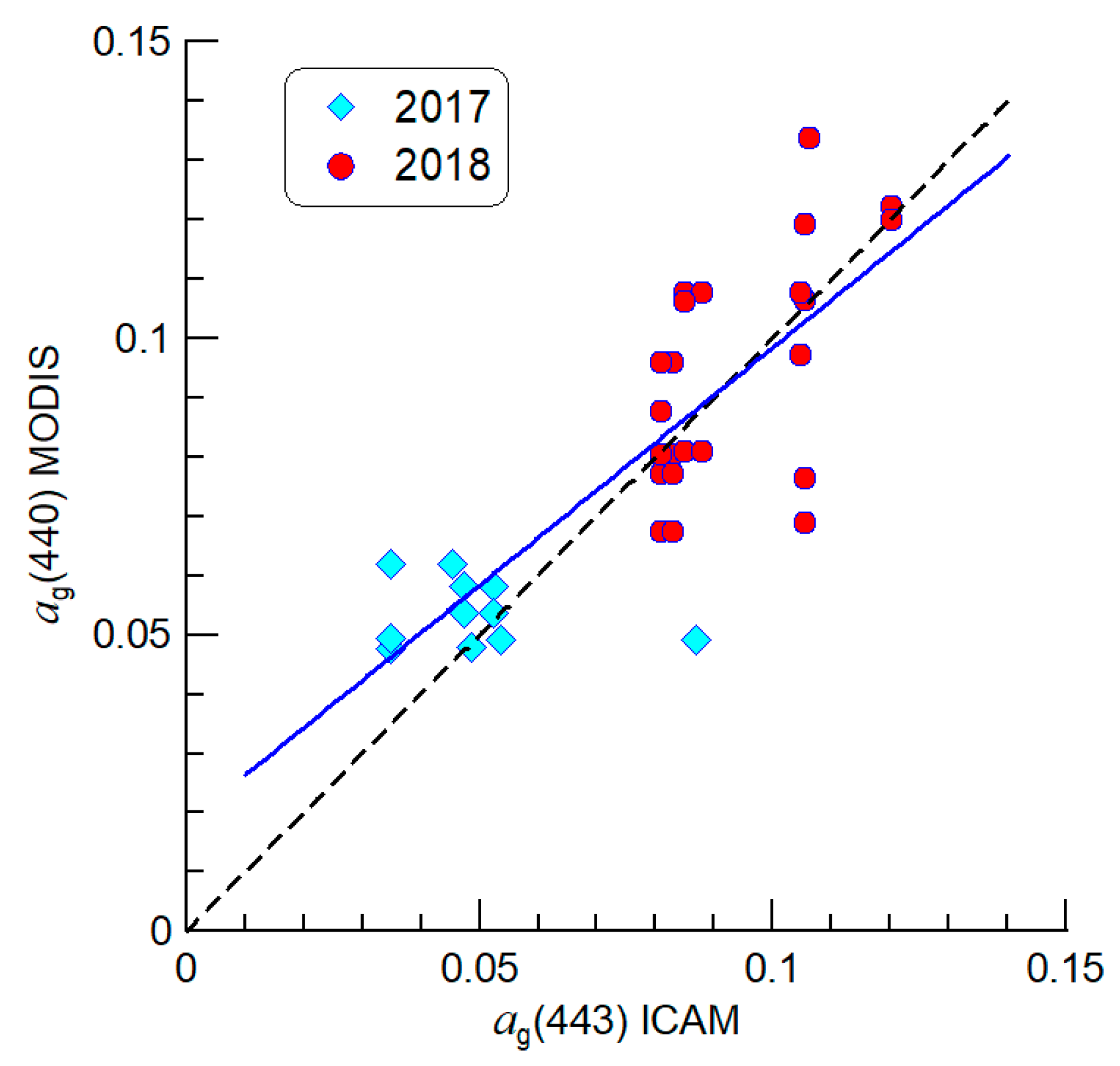
3.3. Comparison between the ag values derived from different measurements
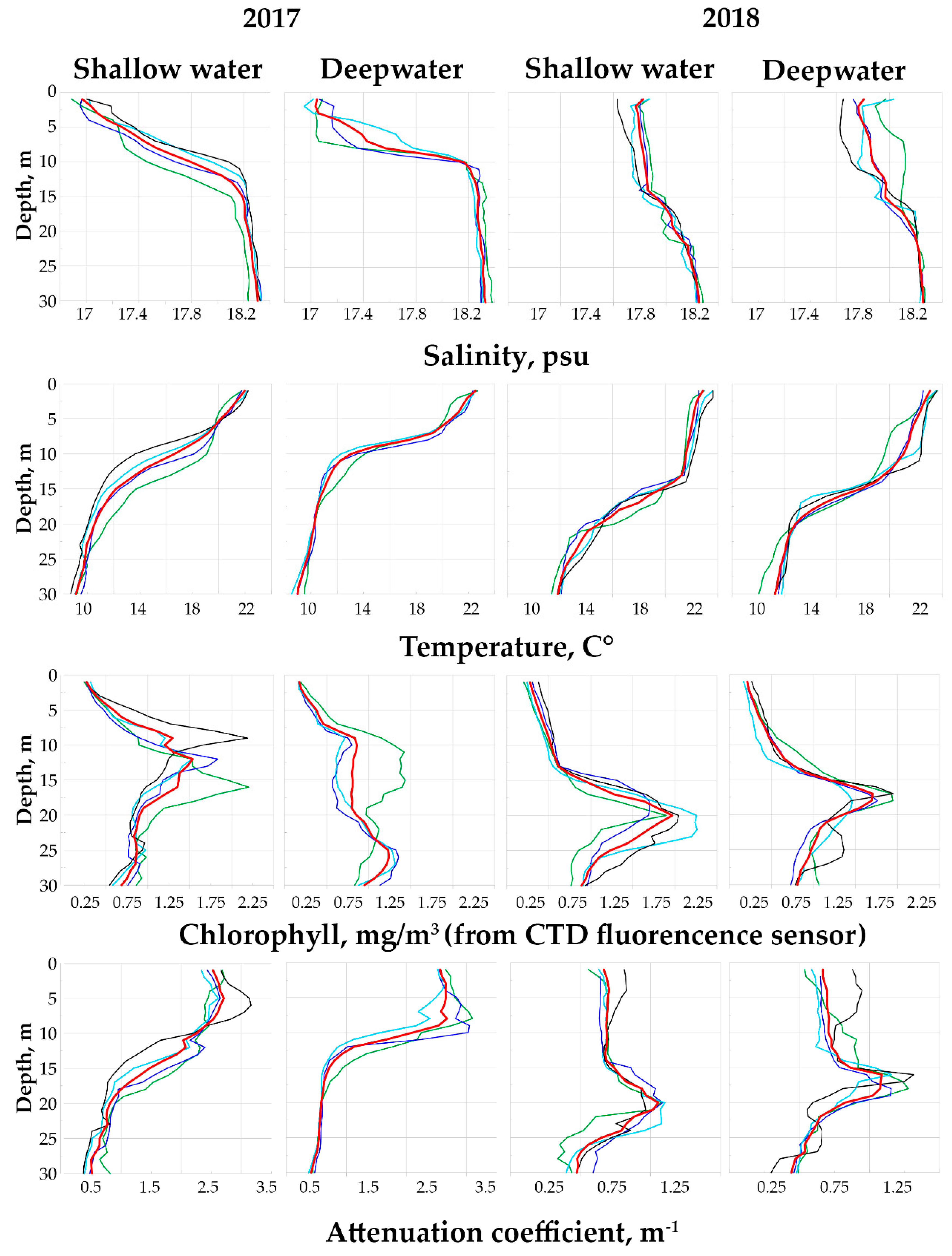
3.4. Comparison of Optical and Hydrological Data
4. Discussion
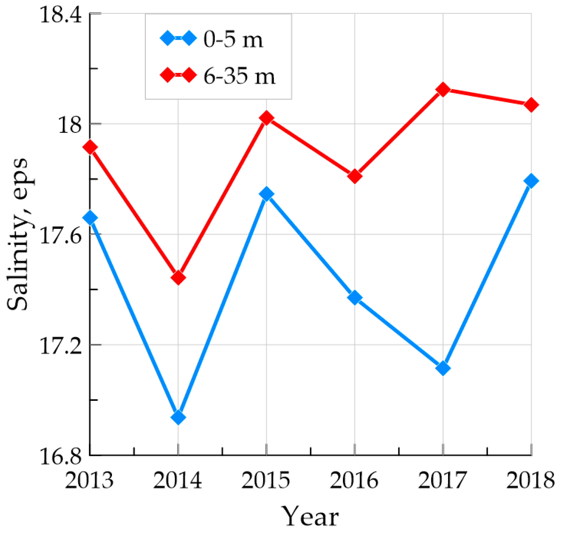
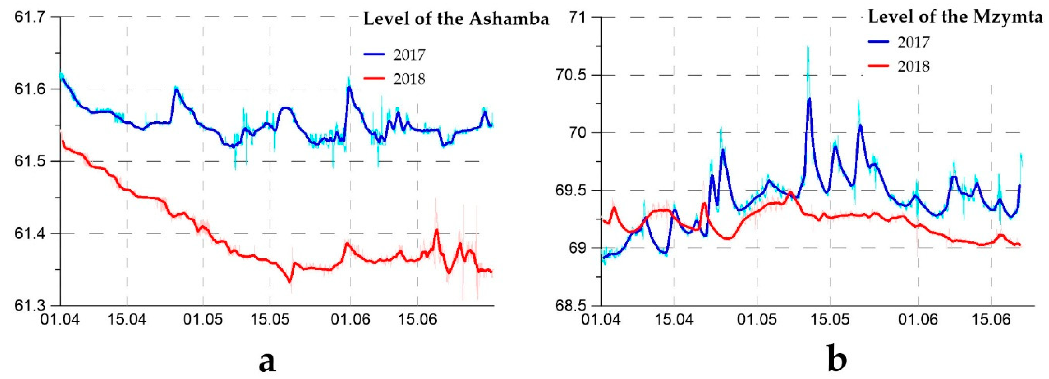
4.1. Interannual Salinity Measurements
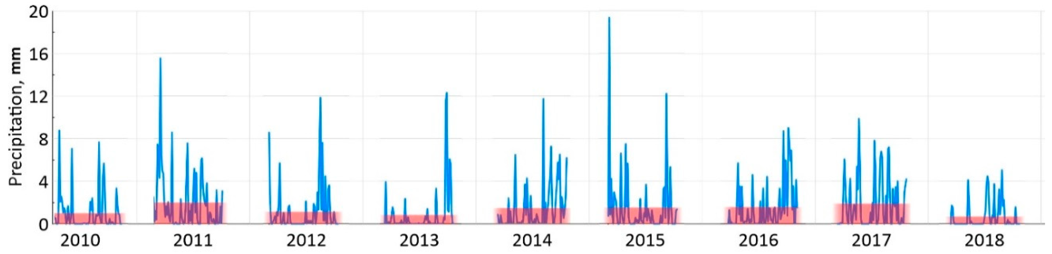
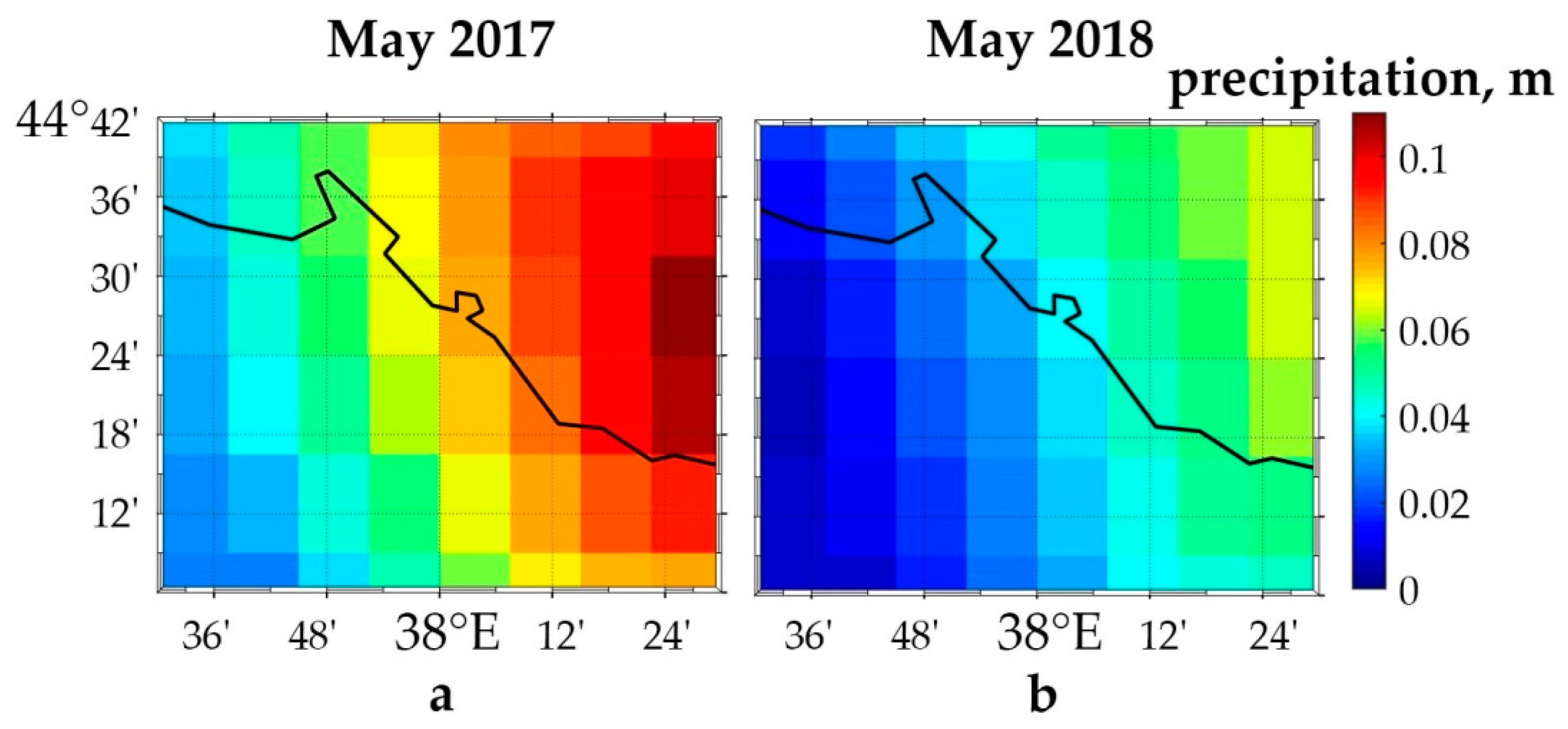
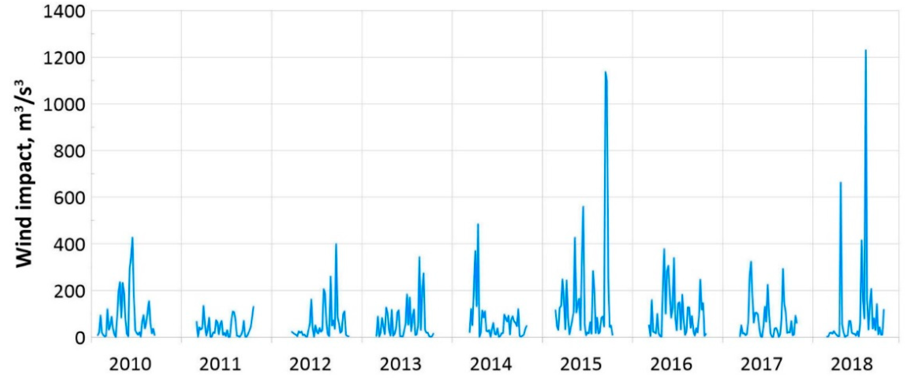
4.2. Precipitation and Wind
4.3. Main Results and Conclusion
Author Contributions
Funding
Acknowledgments
Conflicts of Interest
References
- Burenkov, V.I.; Kelbalikhanov, B.F.; Kopelevich, O.V. Methods of measurements of the seawater optical properties. In Ocean Optics; Monin, A.S., Ed.; Nauka: Moscow, Russia, 1983; Volume 1, pp. 131–139. [Google Scholar]
- Kopelevich, O.V.; Rusanov, S.J.; Nosienko, N.M. Light absorption by sea water. In Hydrophysical and Hydrooptical Investigations in the Atlantic and Pacific Oceans in View of Results of the 5th Cruise of r/v “Dimitry Mendeleyev”; Nauka: Moscow, Russia, 1974; pp. 107–112. [Google Scholar]
- Kopelevich, O.V.; Burenkov, V.I. On the relationship between spectral light attenuation coefficients of sea water, phytoplankton pigments and yellow substances. Okeanology 1977, 17, 427–433. [Google Scholar]
- Kopelevich, O.V.; Lyutsarev, S.V.; Rodionov, V.V. The spectral absorption of light by yellow substance in ocean water. Oceanology 1989, 29, 409–414. [Google Scholar]
- Kalle, K. The problem of Gelbstoff in the sea. Oceanogr. Mar. Biol. Annu. Rev. 1966, 4, 91–104. [Google Scholar]
- Højerslev, N.K. On the origin of yellow substance in the marine environment. Oceanogr. Rep. Univ. Cph. Inst. Phys. 1980, 42, 1–35. [Google Scholar]
- Bricaud, A.; Morel, A.; Prieur, L. Absorption by dissolved organic matter of the sea (yellow substance) in the UV and visible domains. Limnol. Oceanogr. 1981, 26, 43–53. [Google Scholar] [CrossRef]
- Carder, K.L.; Steward, R.G.; Harvey, G.R.; Ortner, P.B. Marine humic and fulvic acids: Their effects on remote sensing of ocean chlorophyll. Limnol. Oceanogr. 1989, 34, 68–81. [Google Scholar] [CrossRef]
- Wozniak, B.; Dera, J. Light Absorption in Sea Water; Springer: New York, NY, USA, 2007. [Google Scholar]
- Koblentz-Mishke, O.I.; Wozniak, B.; Ochakovskiy, Y.E. Utilisation of Solar Energy in the Photosynthesis of the Baltic and Black Sea Phytoplankton; Izd. Inst. Okeanol.; AN SSSR: Moscow, Russia, 1985. [Google Scholar]
- Koblentz-Mishke, O.I.; Wozniak, B.; Kaczmarek, S.; Konovalov, B.V. The assimilation of light energy by marine phytoplankton. Part 1. The light absorption capacity of the Baltic and Black Sea phytoplankton (methods; relation to chlorophyll concentration). Okeanology 1995, 37, 145–169. [Google Scholar]
- Churilova, T.; Berseneva, G. Absorption of light by phytoplankton, detritus, and dissolved organic substances in the coastal region of the Black Sea (July–August 2002). Phys. Oceanogr. 2004, 14, 221–233. [Google Scholar] [CrossRef]
- Suslin, V.; Churilova, T. A regional algorithm for separating light absorption by chlorophyll-a and coloured detrital matter in the Black Sea, using 480–560 nm bands from ocean colour scanners. Int. J. Remote Sens. 2016, 37, 4380–4400. [Google Scholar] [CrossRef]
- Kopelevich, O.V.; Burenkov, V.I.; Sheberstov, S.V.; Vazyulya, S.V.; Kravchishina, M.D.; Pautova, L.; Silkin, V.A.; Artemiev, V.A.; Grigoriev, V. Satellite monitoring of coccolithophore blooms in the Black Sea from ocean color data. Remote Sens. Environ. 2014, 146, 113–123. [Google Scholar] [CrossRef]
- Kopelevich, O.V.; Burenkov, V.I.; Sheberstov, S.V. Case Studies of Optical Remote Sensing in the Barents Sea. In Remote Sensing of the European Seas; Springer: Dordrecht, The Netherlands, 2008; pp. 53–66. [Google Scholar]
- Kopelevich, O.V.; Sheberstov, S.V.; Burenkov, V.I.; Vazyulya, S.V.; Pautova, L.A.; Silkin, V.A. New data about coccolithophore blooms in the Black Sea from satellite data. In Proceedings of the YII International Conference «Current problems in Optics of Natural Waters», St.-Peterburg, Russia, 10–14 September 2013; pp. 10–14. [Google Scholar]
- Kopelevich, O.V.; Burenkov, V.I.; Sheberstov, S.V.; Vazulya, S.V.; Sahling, I.V. Coccolithophore Blooms in the North-Eastern Black Sea. In Proceedings of the Twelfth International Conference on the Mediterranean Coastal Environment, Varna, Bulgaria, 6–10 October 2015; MEDCOAST, Mediterranean Coastal Foundation: Dalyan, Turkey, 2015; Volume 1, pp. 363–374. [Google Scholar]
- Thierstein, H.R.; Young, J.R. Coccolithophores—From Molecular Processes to Global Impact; Springer: Berlin, Germany, 2004. [Google Scholar]
- Kopelevich, O.V.; Sahling, I.V.; Vazyulya, S.V.; Glukhovets, D.I. Bio-Optical Characteristics of the Seas, Surrounding the Western part of Russia, from Data of the Satellite Ocean Color Scanners of 1998–2017; Burenkov, V.I., Karalli, P.G., Eds.; OOO «VASh FORMAT»: Moscow, Russia, 2018. [Google Scholar]
- Kopelevich, O.V.; Sahling, I.V.; Vazyulya, S.V.; Glukhovets, D.I.; Sheberstov, S.V.; Burenkov, V.I.; Karalli, P.G.; Yushmanova, A.V. Atlas “Bio-Optical Characteristics of the Seas, Surrounding the Western part of Russia, from Data of the Satellite Ocean Color Scanners of 1998–2017”. Available online: http://optics.ocean.ru/ (accessed on 30 June 2019).
- Pogosyan, S.I.; Durgaryan, A.M.; Konyukhov, I.V.; Chivkunova, O.B.; Merzlyak, M.N. Absorption spectroscopy of microalgae, cyanobacteria, and dissolved organic matter: Measurements in an integrating sphere cavity. Oceanology 2009, 49, 866–871. [Google Scholar] [CrossRef]
- Podymov, O.I.; Zatsepin, A.G. Seasonal anomalies of water salinity in the Gelendzhik region of the Black Sea according to shipborne monitoring data. Oceanology 2016, 56, 342–354. [Google Scholar] [CrossRef]
- Glukhovets, D.I.; Sheberstov, S.V.; Kopelevich, O.V.; Zaytseva, A.F.; Pogosyan, S.I. Measuring the sea water absorption factor using integrating sphere. Light Eng. 2018, 26, 120–126. [Google Scholar] [CrossRef]
- Artemiev, V.A.; Taskaev, V.R.; Burenkov, V.I.; Grigoriev, A.V. Universal compact meter of vertical distribution of light attenuation. In Comprehensive Studies of the World Ocean: Project “Meredian”, Part 1. Atlantic Ocean; Nauka: Moscow, Russia, 2008. [Google Scholar]
- Dee, D.P.; Uppala, S.M.; Simmons, A.J.; Berrisford, P.; Poli, P.; Kobayashi, S.; Andrae, U.; Balmaseda, M.A.; Balsamo, G.; Bauer, P.; et al. The ERA-Interim reanalysis: Configuration and performance of the data assimilation system. Q. J. R. Meteorol. Soc. 2011, 137, 553–597. [Google Scholar] [CrossRef]
- Emersit Data. Available online: http://www.emercit.com/ (accessed on 30 June 2019).
- NASA’s OceanColor Web. Available online: https://oceancolor.gsfc.nasa.gov/ (accessed on 30 June 2019).
- Werdell, P.J.; McKinna, L.I.W.; Boss, E.; Ackleson, S.G.; Craig, S.E.; Gregg, W.W.; Lee, Z.; Maritorena, S.; Roesler, C.S.; Rousseaux, C.S.; et al. An overview of approaches and challenges for retrieving marine inherent optical properties from ocean color remote sensing. Prog. Oceanogr. 2018, 160, 186–212. [Google Scholar] [CrossRef]
- Sheberstov, S.V. System for batch processing of oceanographic satellite data. Mod. Probl. Remote Sens. Earth Space 2015, 12, 154–161. [Google Scholar]
- Gordon, H.R. Can the Lambert–Beer law be applied to the diffuse attenuation coefficient of ocean water? Limnol. Oceanogr. 1989, 34, 1389–1409. [Google Scholar] [CrossRef]
- Burenkov, V.I.; Ershova, S.V.; Kopelevich, O.V.; Sheberstov, S.V.; Shevchenko, V.P. An Estimate of the Distribution of Suspended Matter in the Barents Sea Waters on the Basis of the SeaWiFS Satellite Ocean Color Scanner. Oceanology 2001, 41, 622–628. [Google Scholar]
- Pope, R.M.; Fry, E.S. Absorption spectrum (380–700 nm) of pure water. I. Integrating cavity measurements. Appl. Opt. 1997, 36, 8710–8723. [Google Scholar] [CrossRef] [PubMed]


| Station | ICAM | MODIS (Rrs) | From Kd |
|---|---|---|---|
| At depth of 50 m | 0.081 | 0.076 (−6%) | 0.074 (−9%) |
| At depth of 1500 m | 0.085 | 0.111 (+30%) | 0.066 (−22%) |
| Shallow Water | ||||||
| Depth, m | ag (m−1) | S (psu) | T (°C) | Chl (mg∙m−3) | Ncoc (× 106 Cells/L) | c (m−1) |
| 2017 | ||||||
| Above | 0.10 ±0.02 (11) | 17.1 ± 0.2 (23) | 21.3 ± 1 (23) | 0.66 ± 0.3 (23) | 6.7 ± 2 (23) | 2.3 ± 0.2 (23) |
| Maximum F_chl (8–17 m) | 0.13 ± 0.02 (9) | 18.0 ± 0.2 (12) | 14.2 ± 1 (12) | 2.1 ± 0.7 (12) | 7.0 ± 2.3 (12) | 2.3 ± 0.4 (12) |
| Below | 0.13 ± 0.03 (3) | 18.3 ± 0.1 (13) | 10.3 ± 1 (13) | 1.02 ± 0.3 (13) | 0.57 ± 0.7 (13) | 0.8 ± 0.3 (13) |
| 2018 | ||||||
| Above | 0.16 ± 0.03 (10) | 17.8 ± 0.1 (10) | 22.7 ± 1 (10) | 0.3 ± 0.03 (5) | 0.51 ± 0.1 (4) | 0.70 ± 0.1 (10) |
| Maximum F_chl (17–21 m) | 0.25 ± 0.02 (4) | 18.1 ± 0.1 (4) | 15.3 ± 0.7 (4) | 2.08 ± 0.9 (4) | 0.46 ± 0.3 (4) | 1 ± 0.1 (4) |
| Below | 0.16 ± 0.04 (5) | 18.3 ± 0.1 (5) | 11.6 ± 1 (5) | 1.72 ± 0.3 (2) | 0.20 ± 0.2 (2) | 0.5 ± 0.2 (5) |
| Deep Water | ||||||
| Depth, m | ag (m−1) | S (psu) | T (°C) | Chl (mg∙m−3) | Ncoc (× 106 cells/L) | с (m−1) |
| 2017 | ||||||
| Above | 0.07 ± 0.01 (5) | 17.2 ± 0.2 (8) | 21.7 ± 1 (8) | 0.5 ± 0.15 (8) | 6.3 ± 1.6 (8) | 2.6 ± 0.1 (8) |
| Maximum F_chl (8–17 m) | 0.16 (1) | 18.2 ± 0.1 (4) | 12.4 ± 0.8 (4) | 1.06 ± 0.5 (4) | 6.4 ± 3.1 (4) | 1.8 ± 1 (4) |
| Below | 0.13 ± 0.02 (3) | 18.3 ± 0.1 (6) | 8.7 ± 0.9 (6) | 0.92 ± 0.6 (6) | 0.1 ± 0.07 (6) | 0.4 ± 0.1 (6) |
| 2018 | ||||||
| Above | 0.16 ± 0.04 (14) | 17.6 ± 0.2 (14) | 22.3 ± 1 (14) | 0.35 ± 0.2 (6) | 0.8 ± 0.30 (4) | 0.7 ± 0.1 (14) |
| Maximum F_chl (17–21 m) | 0.26 ± 0.05 (4) | 18.1 ± 0.1 (5) | 14.5 ± 1 (5) | 2.03 ± 0.3 (5) | 0.7 ± 0.43 (5) | 1.2 ± 0.2 (5) |
| Below | 0.18 ± 0.03 (6) | 18.3 ± 0.1 (5) | 11 ±1.3 (5) | 1.06 ± 0.3 (2) | 0.22 (1) | 0.4 ± 0.1 (5) |
| Year | 2010 | 2011 | 2012 | 2013 | 2014 | 2015 | 2016 | 2017 | 2018 |
|---|---|---|---|---|---|---|---|---|---|
| Precipitation (mm) | 1.00 | 2.00 | 1.13 | 0.83 | 1.47 | 1.52 | 1.57 | 1.89 | 0.68 |
| ∑Precipitation (mm) | 72.0 | 144.2 | 81.1 | 59.5 | 105.6 | 109.7 | 113.1 | 136.4 | 48.8 |
| Year | 2010 | 2011 | 2012 | 2013 | 2014 | 2015 | 2016 | 2017 | 2018 |
|---|---|---|---|---|---|---|---|---|---|
| Average V3 (m3/s3) | 85.2 | 39.3 | 55.6 | 63.2 | 69.5 | 163.0 | 100.9 | 70.9 | 96.6 |
| ∑ V3 (m3/s3) | 3579 | 1652 | 2337 | 2654 | 2920 | 6846 | 4238 | 2978 | 4058 |
© 2019 by the authors. Licensee MDPI, Basel, Switzerland. This article is an open access article distributed under the terms and conditions of the Creative Commons Attribution (CC BY) license (http://creativecommons.org/licenses/by/4.0/).
Share and Cite
Yushmanova, A.; Kopelevich, O.; Vazyulya, S.; Sahling, I. Inter-Annual Variability of the Seawater Light Absorption in Surface Layer of the Northeastern Black Sea in Connection with Hydrometeorological Factors. J. Mar. Sci. Eng. 2019, 7, 326. https://doi.org/10.3390/jmse7090326
Yushmanova A, Kopelevich O, Vazyulya S, Sahling I. Inter-Annual Variability of the Seawater Light Absorption in Surface Layer of the Northeastern Black Sea in Connection with Hydrometeorological Factors. Journal of Marine Science and Engineering. 2019; 7(9):326. https://doi.org/10.3390/jmse7090326
Chicago/Turabian StyleYushmanova, Anna, Oleg Kopelevich, Svetlana Vazyulya, and Inna Sahling. 2019. "Inter-Annual Variability of the Seawater Light Absorption in Surface Layer of the Northeastern Black Sea in Connection with Hydrometeorological Factors" Journal of Marine Science and Engineering 7, no. 9: 326. https://doi.org/10.3390/jmse7090326