Evaluating the Performance of a Dual-Frequency Multibeam Echosounder for Small Target Detection

Abstract

With rising interest in marine renewable energy (MRE) associated with offshore wind, waves, and tidal flows, the effects of device placement on changes in animal behaviour require proper assessment to minimise environmental impacts and inform decision making. High-frequency multibeam echosounders, or imaging sonars, can be used to observe and record the underwater movement and behaviour of animals at a fine scale (tens of metres). However, robust target detection and tracking of closely spaced animals are required for assessing animal–device and predator–prey interactions. Dual-frequency multibeam echosounders combine longer detection ranges (low frequency) with greater detail (high frequency) while maintaining a wide field of view and a full water column range compared to acoustic or optical cameras. This study evaluates the performance of the Tritech Gemini 1200ik imaging sonar at 720 kHz (low frequency) and 1200 kHz (high frequency) for small target detection with increasing range and the ability of the two frequency modes to discriminate between two closely spaced targets using a 38.1 mm tungsten carbide acoustic calibration sphere under controlled conditions. The quality of target detection decreases for both modes with increasing range, with a 25 m limit of detection at high frequency and a low-frequency mode able to detect the target up to 30 m under test conditions in shallow water. We quantified the enhanced performance of the high-frequency mode in discriminating targets at short ranges and improved target detection and discrimination at high ranges in the low-frequency mode.

1. Introduction

Multibeam echosounders have been used extensively for water column imaging globally. Different frequencies have been employed to study diving seabirds, marine mammals, fish, and abiotic objects, like shipwrecks, mines, or coral reefs. Rising interest in marine renewable energy due to shifting energy demands, concerns about fossil fuels, and government net-zero initiatives have led to increased stakeholder interest in offshore wind, tidal stream, and wave energy.

Previous studies have used high-resolution and high-frequency (kHz and MHz) multibeam sonars to detect and track animal movement [1,2]; although highly effective, these studies can be limited due to their short sampled ranges of around 10 metres and relatively narrow swath. The short range is a result of the frequency used and high sound attenuation, thus making imaging the entire water column or detecting and tracking of moving targets above or below areas of interest, like around rotor blades or turbine structures, difficult. With low-frequency multibeam echosounders, a greater range is provided at the cost of a lower resolution of the targets [2,3,4,5,6,7].

New high-frequency multibeam echosounders allow for capturing very-high-resolution data, of almost image-like quality, of large marine mammals [8] and fish [2,9], allowing a plethora of new classification methods with high degrees of success to identify target species in multibeam data [10,11]. To achieve the desired outputs for answering ecological questions, it is of great importance to understand how targets are detected within the multibeam swath.

There are two main ways in which multibeam echosounders are tested and evaluated: laboratory-based calibration and field trials.

Calibration often uses a tank or a controlled environment to characterise source level, beam patterns, and the ability to resolve the angular position of a target [12,13,14]. In comparison, field testing uses the multibeam echosounder in situ to assess detection capabilities on known or opportunistic abiotic/biotic targets [15,16]. Evaluating detection capabilities, particularly as a function of range, target type, and environmental conditions, is of great importance for the application of multibeam echosounders to water column imaging.

The Canadian Offshore Energy Research Association (OERA) Pathway Program field-tested detection capabilities in the high flow conditions of a Tritech Gemini 720i (720 kHz) and Teledyne Blueview M900-2250 (900/2250 kHz) with the eventual goal of monitoring animals around tidal stream turbines. The instruments were mounted on a boat, orientated with an oblique horizontal swath. Three objects (lead fishing weight, basalt rock, and V-Wing glider) were drifted below a second boat through the ensonified area of both multibeam echosounders. The data were inspected manually via the manufacturer software (Tritech Genesis version 1.7.4.108) for detections by experts and instruments cross compared to investigate detections [15,16]. These types of field studies go hand in hand with more specific evaluations of multibeam instruments aimed at understanding specific targets like a particular fish species or visual signatures [8,9], but previous studies have often overlooked the potential effect of surrounding factors like noise caused by turbid or turbulent flows, potential suspended sediments altering reflection, and target size and orientation that might influence uncalibrated multibeam echosounder readings [12,13].

With the increase in the resolution of almost image-like quality for larger targets [8,9] the interest in classifying the recorded target data into specific animal groups has become of increased interest. The morphology of various targets like fish schools, seals, cetaceans, and sharks has been studied with other multibeam echosounders, but comparative metrics to assess the target are often lacking for imaging sonars [12,17,18,19]. Many studies have used single-frequency multibeam echosounders with varying resolutions to investigate animal behaviour, but barely a few have shown and analysed the capabilities of dual-frequency echosounders with the main focuses being on fish size, changes in animal behaviour around MRE devices, and group composition estimations [2,4,5]. Some of these studies focus exclusively on river-bound fish and as a means to measure their length [20,21,22], meaning that the use of dual-frequency sonars for marine animals is comparatively unexplored, though several studies have investigated the imaging capabilities of different multibeam imaging sonars for the purpose of species identification [8,9,10]. Multibeam sonars have shown great effectiveness in estimating fish size compared to baited trap sampling or camera-based techniques, especially during diurnal and nocturnal sampling times and/or turbid environments with high flow speeds and particle suspension [21,22].

Most multibeam echosounder studies do not calibrate the instrument and use a relative measure of backscatter confounding comparisons between studies [17]. Site-specific factors like flow speed, animal abundance, wave-generated noise, and seabed composition can alter the returns and visibility of targets within the swath and are said to be some of the most hindering factors in allowing comparisons between multiple datasets [17,18,19]. Understanding how factors like target range or separation between targets influence detection is of great importance to the application of imaging sonar for the purpose of collecting and categorising relevant data on marine life throughout the water column at specific points of interests like MRE devices, tidal streams, and potential nursery grounds.

This study evaluates the performance of a dual-frequency multibeam echosounder with the eventual application of detecting animals in the water column and measuring target behaviour, e.g., size, shape, velocity, direction, and location in the water column. Combining the longer-range target detection capability expected in a low-frequency mode with the enhanced details in high frequency, the study seeks to quantify the performance of the integrated use of these modes using a new dual-frequency multibeam imaging sonar.

Additionally, this study provides the framework for a cost-efficient evaluation of the capabilities of a dual-frequency multibeam imaging sonar. It combines established target suspension and echosounder calibration techniques [19] with previous field study techniques investigating the detection capabilities of multibeam echosounders at different ranges and the ability to detect calibration spheres, used as a proxy of fish swim bladders [14,15,16]. The experimental methodology developed is designed to be transferable, using standard targets and establishing standard procedures to allow evaluation against other instruments and in different conditions in the future.

Multibeam Echosounder Operation

Multibeam echosounders transmit a burst of sound commonly referred to as a pulse or ping. As the pulse travels outwards from a point source, it increases volumetrically, while the intensity decreases with distance due to energy loss via absorption and an increase in volume (spreading). The pulse duration (in time) and corresponding pulse length (in metres) affect the potential range resolution and the ability of target detection. A short pulse duration allows for a higher target resolution, as the corresponding shorter pulse length allows for an increased range resolution of a target, potentially increasing the distinguishability between multiple closely spaced targets or improving the visibility of notable features like fins, flukes, or body shapes, allowing for an increased chance of successful target classification [13,23,24].

After acoustic waves encounter a density difference (difference in acoustic impedance) such as a potential target, part of the incident energy is scattered and/or reflected, producing reflections that propagate in all directions away from the target depending on its volume, size, and surface smoothness. In general terms, the smoother the surface, the more confined the reflected energy is to follow the direction of the incident wave fronts [22]. Acoustic backscatter can additionally be influenced by the size of the object in relation to the size of the incoming wavelength of the acoustic signal. If the wavelength is far greater than the target length, the resulting backscatter will radiate outward from the target in all directions. The scattered intensity is not equal in all directions and is dependent on the volume of the target. In the case of the target being larger than the incoming signal wavelength, the incoming signal will be reflected based on the angle of incidence. When the target size and wavelength are approximately equal in size, the scattering depends on the geometric and internal structure of the target, i.e., surface roughness, material properties, and composition [23].

Resolution improves with reducing pulse length at the cost of increasing noise relative to the signal, as less acoustic energy is transmitted in a shorter pulse. To overcome the increased noise, in general, more power is needed for transmission. Noise is a term used to describe unwanted signals that are present within the swath, independent of the acoustic signal sent out by the echosounder, and it is a crucial factor to be aware of during data collection. The main sources of noise can be classified into different categories, like physical (wind, wave action, and turbulence), biological (animal noise and movement), artificial (ship noise and other acoustic instruments), and electrical [12,19,25].

Compressed High-Intensity Radar Pulse (CHIRP) [23,24,26] allows for a frequency-modulated broadband sound pulse that aids in improving the Signal-to-Noise Ratio (SNR), a measure of the desired signal compared to the background noise, of the recorded data. It transmits a long pulse across a wide frequency band. In general, the pulse duration is longer compared to a continuous-wave single-frequency pulse, meaning more energy is transmitted into the water column [23]. CHIRP mitigates the negative effects of a longer pulse duration on range resolution via a process called pulse compression. As a CHIRP device receives more information per pulse compared to its standard counterpart, it is able, via pulse compression, to a convert long-duration pulse into narrow pulses with high amplitudes. These narrow pulses can be correlated to a long duration with low power pulse, which increases the available range resolution, even at long pulse durations. The effectivity or quality of a transducer is assessed by the quality factor Q with CHIRP-enabled transducers having on average a lower Q number, indicating a general higher resolution compared to single-frequency (continuous-wave or narrowband) pulses.

2. Materials and Methods

2.1. Experimental Site and Setup

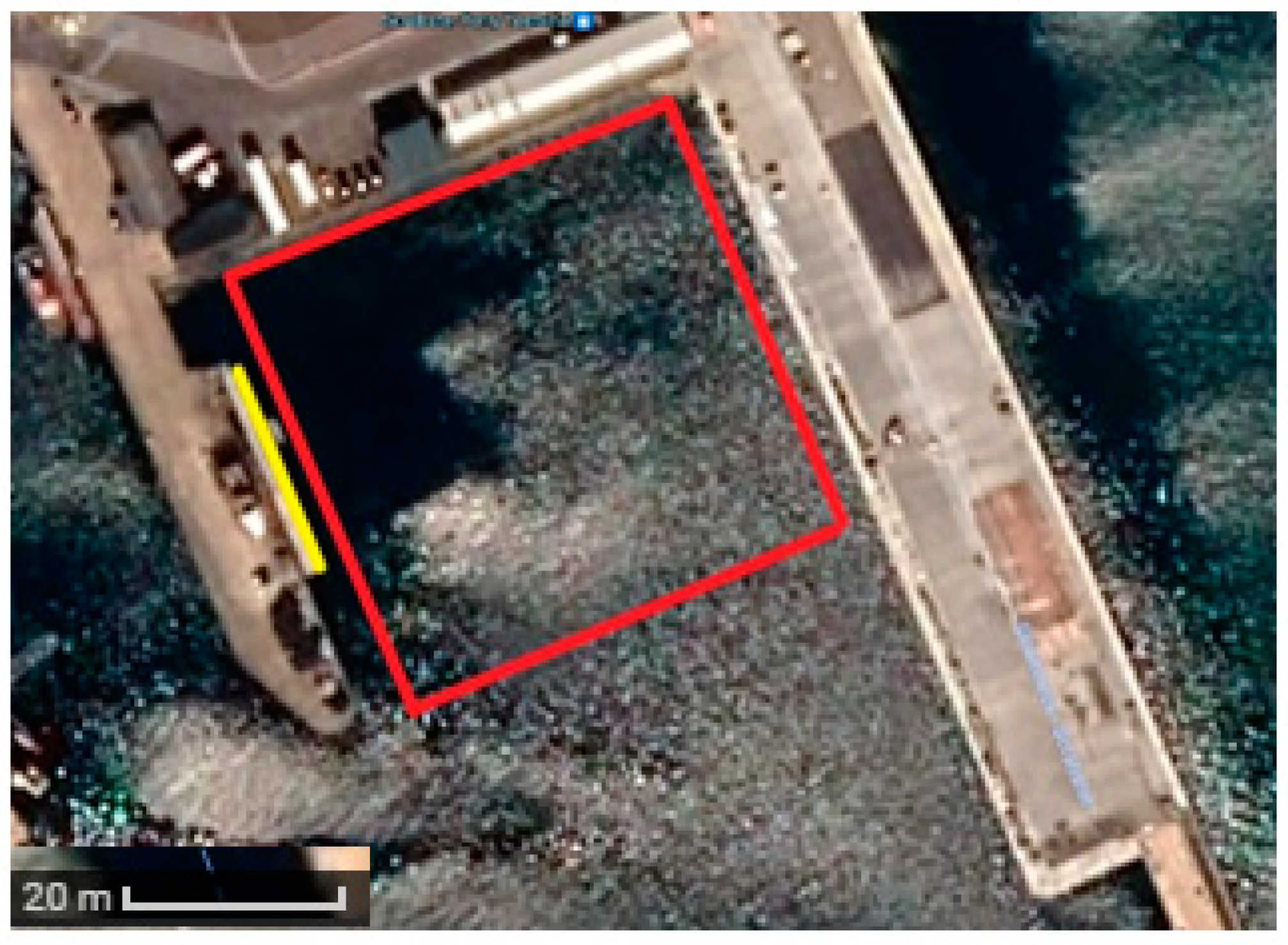
The site of the experiment was at Scrabster Harbour (Caithness, Scotland, UK, Figure 1) with an average depth of 8 m near the pontoon during high tide with increasing depths to an average of 12 m. A Tritech Gemini 1200ik dual-frequency imaging sonar with either a 1200 kHz (high frequency) or a 720 kHz (low frequency) mode was used for data collection. Changing the frequency mode of the 1200ik changes the number of beams and the range resolution; for high frequency, the number of beams was 1024 with a range bin resolution of 1696, and for low frequency, the number of beams was 512 with a range bin resolution of 1058. A buoy with a tungsten carbide sphere was used as an assumed target, which was moved across the harbour and away from the multibeam to investigate its detection and separation capabilities.

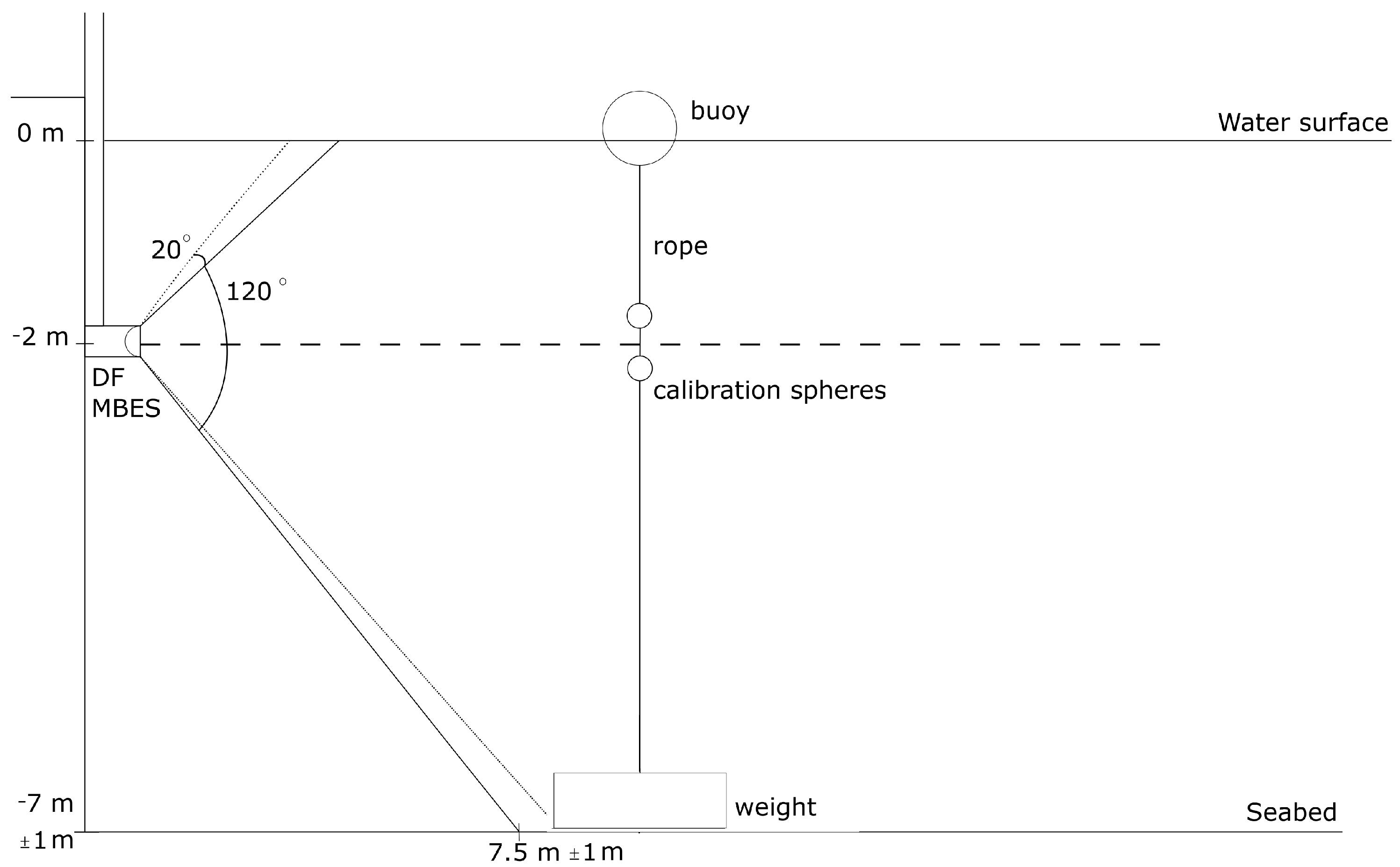
The dual-frequency multibeam was placed in a vertical orientation with the 120° along-swath direction orientated vertically (Figure 2) and the 20° (low-frequency mode)/12° (high-frequency mode) across-swath direction orientated horizontally. The change in across-swath beamwidth between frequency modes may affect target visibility. The target was acoustically centred in the horizontal (across-swath) direction using an iterative process of incrementally varying the horizontal (azimuth) angle of the sonar in approximately 2° steps, recording data for a period of 60 s and selecting the section of the dataset with the highest intensity measure of the target during post processing, which was identified as when the target was acoustically centred in the across-swath direction. The multibeam echosounder was facing away from the floating pontoon (Figure 1) towards the distant harbour wall at approximately 40 m.

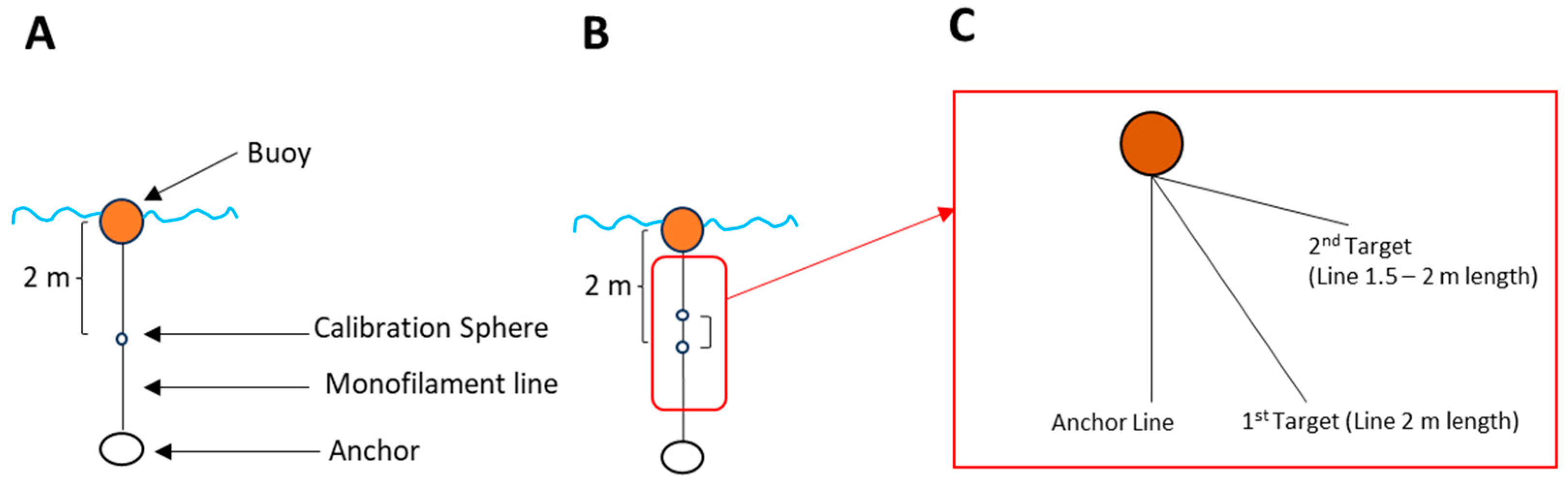
Initially, a single calibration sphere was suspended 2 m below (Figure 2) the surface at the same depth as the multibeam echosounder and at the nadir in the horizontal and vertical (along and across swath, respectively) directions. For investigating the separation distance, a similar setup was used, with two calibration spheres being moved closer together by increasing the length of an additional nylon line on which the 2nd target was suspended (Figure 3). The targets were suspended from the buoy with an anchor using an acoustically transparent monofilament line of 0.25 mm in diameter to reduce the potential interference within the water column [19].

To suspend the spheres within the water column, a similar design to that within the ICES CRR 326 [19] was used, allowing for the manipulation of the spheres. The x and y (horizontal) coordinates were assumed to remain constant over the course of the experiment within the sheltered part of the harbour, with the only change being the vertical (z) distance between the spheres. The anchor was small and low profile aiming for a similarity with the seabed to decrease the potential interference with the target readings from any swath (beamwidth) sidelobes.

Measurements were conducted over several days, and environmental conditions are presented in

Table 1. Environmental factors during the survey days. Water depth was the measured depth at the pontoon.

Date	Wind Speed (ms−1)	Tidal State	Water Depth (m)	Operation
22 April 2022	1.5	High	7.7	SNR, Trial Separation Distance
23 April 2022	2.8	High	8.8	Separation Distance 5, 15 m—repeat of 15, 20 m SNR recording
28 April 2022	1.9	High	10.5	Separation Distance 25 m and repeated 15 m

.

2.2. Experimental Procedure

The experiment was started during high tide at flood to allow for the deepest possible water depth at Scrabster Harbour to minimise possible seabed interference. The 1200ik was clamped to the pontoon pointing towards the opposite harbour wall and was submerged at a 2 m depth. Wind speed, surface conditions, and air temperature were recorded for the final data analysis, while the multibeam echosounder range setting was set to 35 m to not include the strong reflections from the harbour wall located approximately 40 m from the pontoon. Display gain was set to 100% for maximum visibility of the target.

Before the sphere deployment, background noise measurements were taken in both frequency modes for a 3 min period each day of the experimental trials. The buoys were deployed with the aid of a kayak at the relevant ranges from the multibeam and centred before recording for one minute, and the frequency mode was swapped. Seven measurements were taken at the ranges of 1, 5, 10, 15, 20, 25, and 30 m for both frequency modes. To investigate the ability of the 1200ik to separate between two targets, a similar setup was used, but the spheres were only deployed at 5, 15, 25, and 35 m ranges, with 35 m yielding no usable data.

All data captured with the 1200ik were recorded as GLF files with a constant range setting of 35 m and with CHIRP enabled for both frequencies over the duration of the experiment.

2.3. Data Processing and Analysis

As the multibeam is uncalibrated, all backscatter pixel values are relative returns (0–255, arbitrary units). MATLAB R2021a was used for all data processing as follows:

• A polar plot of the swath showing the maximum intensity over time over the recording period (for one experimental configuration) was created;
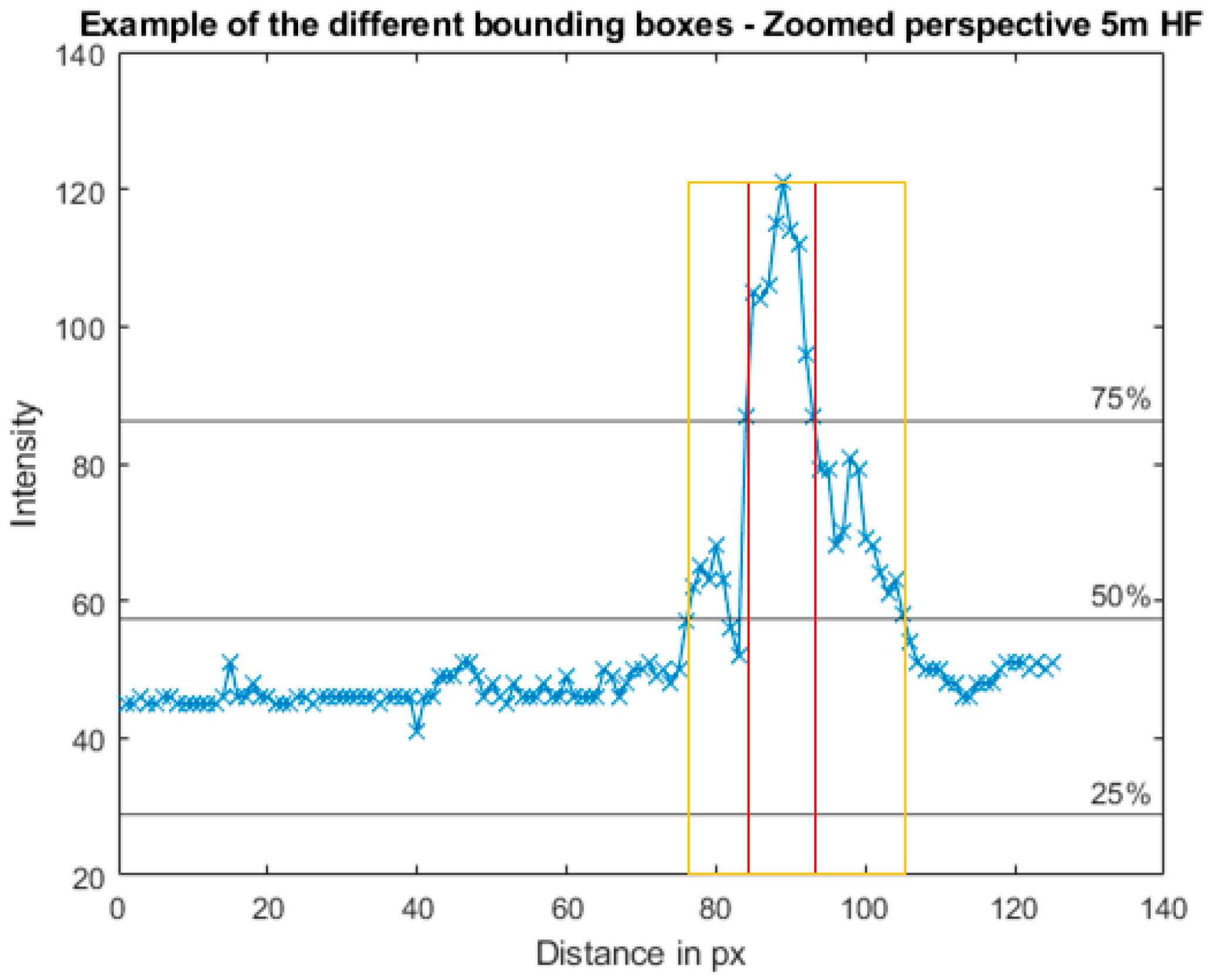
• The region of highest intensity, which corresponds to the midwater target, was identified, and an approximate bounding box was manually defined around it;
• The maximum intensity value and location within that region were identified, and the corresponding frame was used for further data processing;
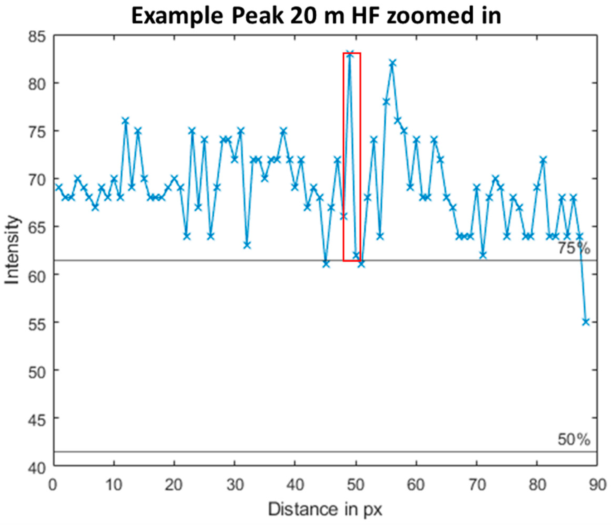
• An intensity plot was created through the centroid of the region both horizontally and vertically;
• A second bounding box was created with its extent determined by the cut-off value of 75% lower intensity than the maximum value in the horizontal and vertical directions. An example of the process is further explained in Figure 4;
• The mean intensity value of the pixels within the bounding box was extracted by investigating the changes in mean intensity of the target over all frames within the bounds of the bounding box.
  • Frames that were determined to contain a peak in the target’s intensity over time were extracted.
  • The mean intensity of the target values of each of those frames was extracted before the mean over time was determined.

It was decided to use the mean of the intensity within the bounding box as this study aimed to look at the change of the overall target. It was assumed that the mean intensity of the target provided a better evaluation of effectiveness than comparing peak intensities.

2.3.1. Bounding Box Extent

A value of 75% of the maximum intensity of the target was used as a cut-off point for the width and length of the bounding box. The effect of changing the cut-off value for the intensity is shown in Figure 4, and representative ranges of 5, 15, and 25 m in high frequency are shown in

Table 2. Effect of changing the bounding box cut-off value on the mean intensity within the box for high-frequency recordings.

Range in m	Mean Intensity at 75%	Mean Intensity at 50%	Mean Intensity at 25%	Mean Intensity of the Noise
5	105.3	85.2	51.9	48.7
15	68.7	59.8	58.5	58.2
25	68.1	68.6	68.7	71.4

.

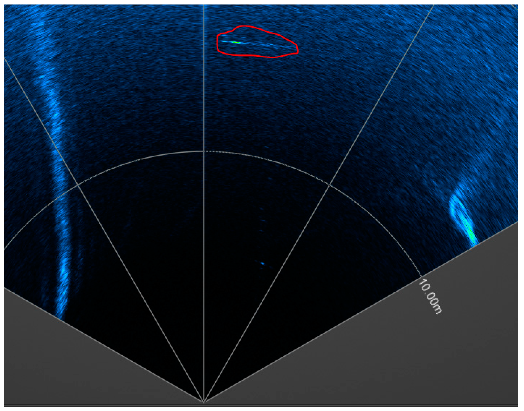
During the data processing for the high-frequency recordings, it was noted that at both the 20 and 25 m ranges, the mean intensity of the signal was found to be lower than the mean intensity of the noise. At these points, the maximum intensity allowed for the likely target to be identified through manual inspection based on the expected location (Figure 5). Additionally, the bounding box cut-off values were below the noise within the recording, requiring manual determination of the bounding box extent. This is one of the main reasons why it was decided to use the mean intensity of the target, as otherwise the target would be marked as visible (based on maximum, not mean), but based on a detection-based algorithm that searches for specific features in mean intensity, the target might have been overlooked, indicating a potential area of future investigation.

2.3.2. Background Recording

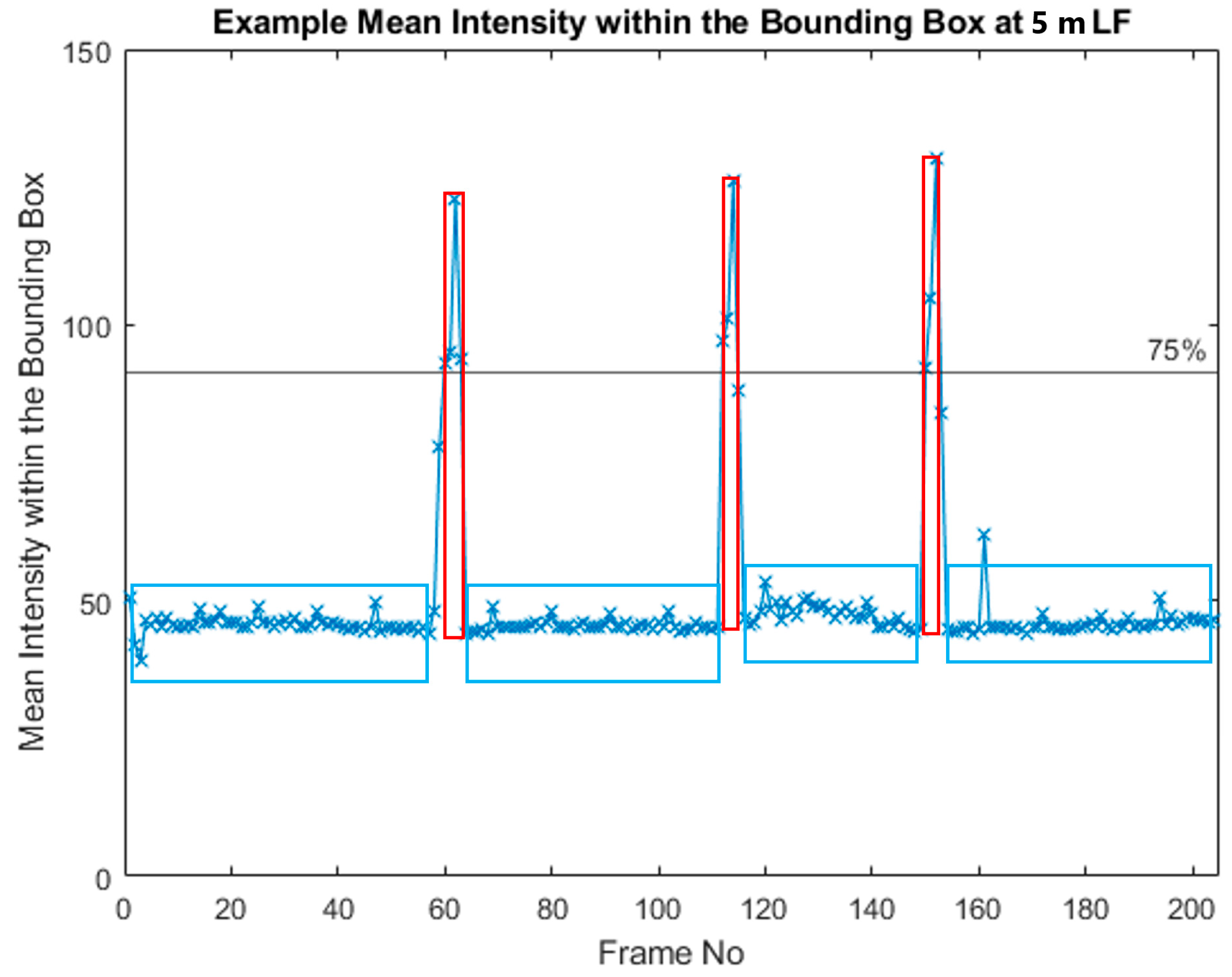
The noise value was determined from one recording at the beginning of the experiment, which recorded the site in both low and high frequency for a minute. 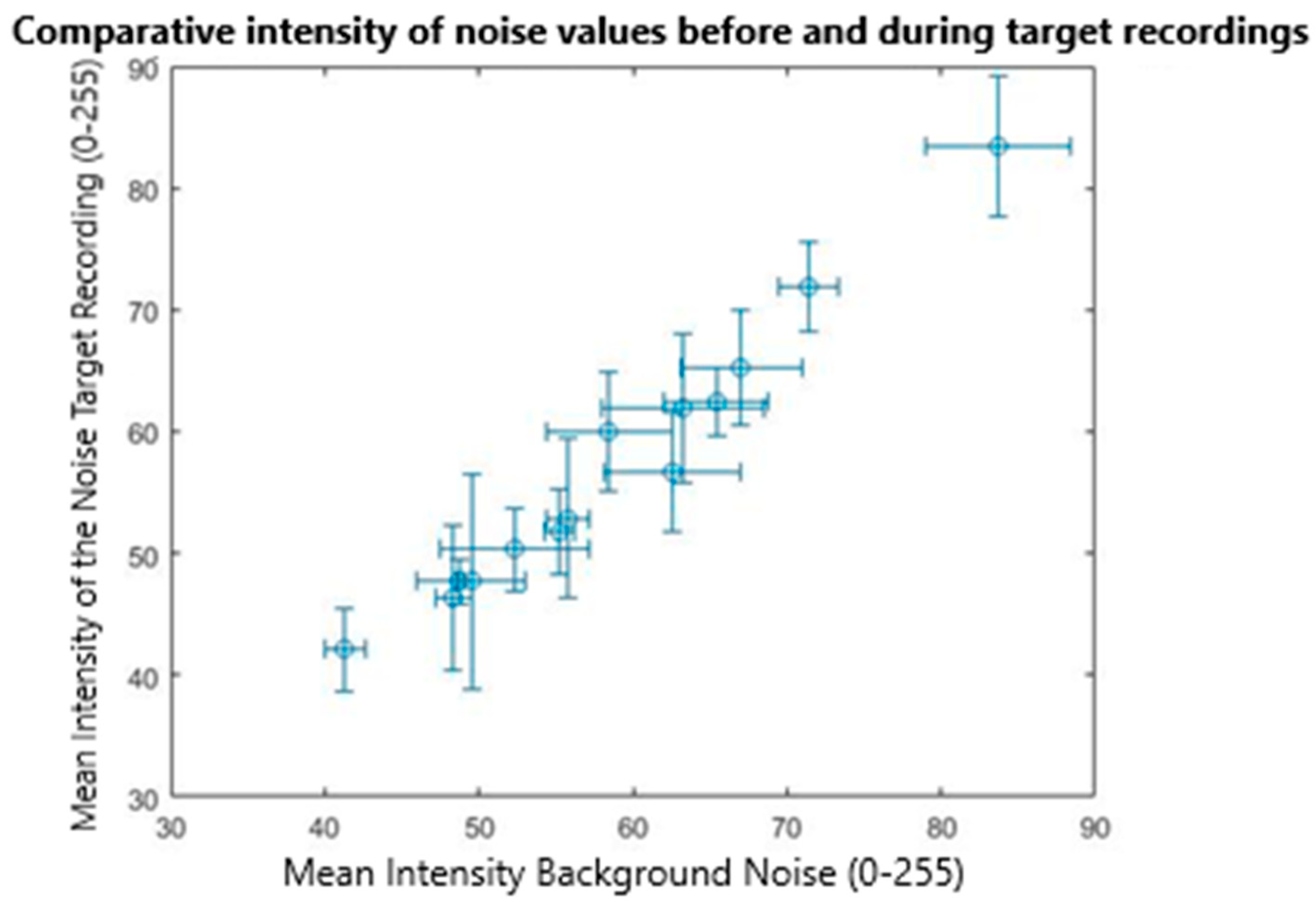The same bounding box used in determining the intensity of each target was placed at the corresponding position within the noise recording, and the mean intensity within the bounding box was calculated, followed by the mean over the duration of the 1 min noise recording (Figure 6). To fully compare the noise levels during and before the experiment, noise levels within the recording were also taken, at the same range as the target, and compared against the pre-recording levels (Figure 7). Based on the potential varying noise levels in the harbour during the experiment, this method was employed to determine if there had been changes in background noise between the pre-recording and the recordings and, if noise occurred, whether it would impact the measurements. The approach is designed to be transferable to support comparison with other studies in future, and it follows methods used to analyse datasets with temporal varying noise but focuses on the multibeam reading of intensity instead of considering a spectral noise analysis.

Encountered noise is suggested to be mainly reverberations of acoustic waves when they encounter biological material or suspended sediments. The recording occurred during flood tide, which may explain the possible increase in background noise as water entering the harbour may have resuspended sediment from the bottom.

It was assumed that the background would not change substantially during the experiment. This was verified by comparing the mean intensity within the bounding box in the background recording against the mean intensity present in the actual recording after the peaks, indicating the target was removed. The signal within the recording that includes the target can be split into three different parts illustrated in Figure 6. Red boxes represent the part of the signal that are attributed to be the target and fall above a 75% cut-off based on the maximum intensity. A 75% cut-off value was used as it presents the most visible part of the target, as the multibeam swath was panned across the study site to acoustically centre the targets in the 12/20° beamwidth. The blue boxes are the background noise that occurs when the target is not within the multibeam swath.

Mean noise intensity values from before the target recording and during the target recording are similar. A slight bias towards an increased noise value from the background recording was determined through Figure 7, with most data points showing a high deviation as the mean noise intensity during the target recordings showed more variation compared to the pre-target noise recordings.

2.3.3. Target Discrimination—Separation Distance

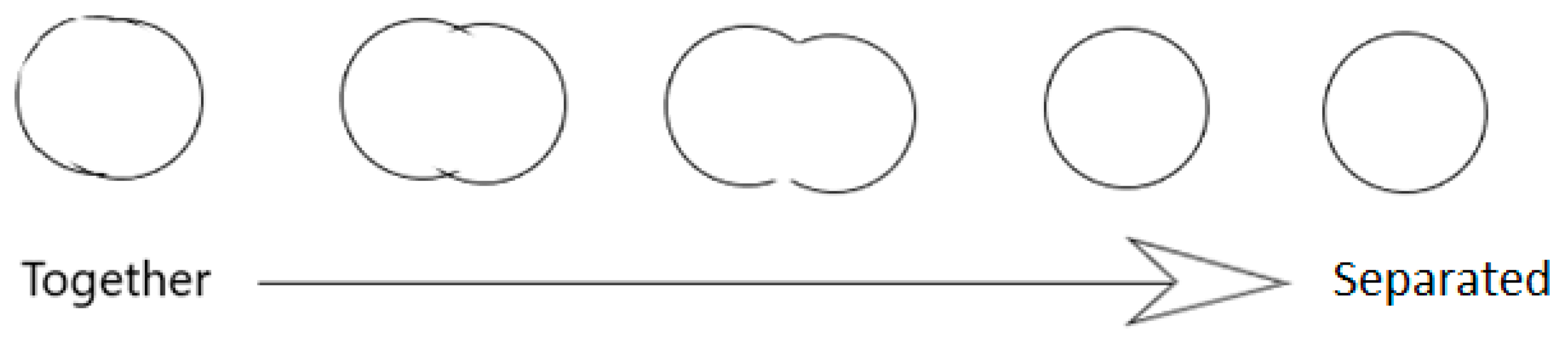
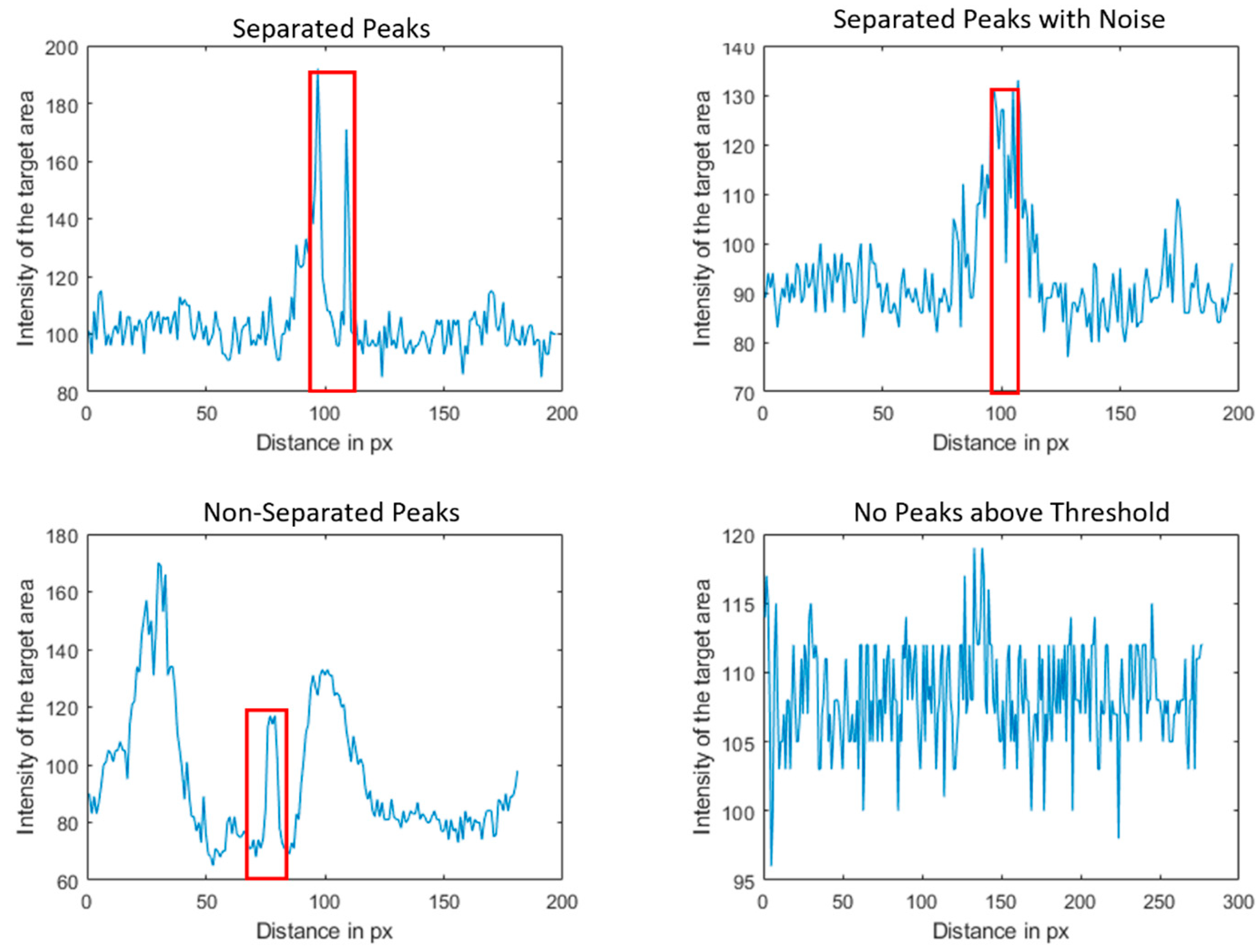
Identifying the separation can be performed using a similar method as above to draw the bounding boxes. Figure 8 shows an example of the potential returns with increasing distance between the two spheres.

The following method was employed to determine the degree of separation:

• An intensity plot that intersects vertically through the centroids of both spheres was generated, as it was assumed that there would be minimal movement (swinging) by the spheres;
• The ‘findpeaks’ function within MATLAB processes the vertical line intersecting the centroid of both spheres and determines the resulting peaks based on the following parameters:
  • Prominence—the minimum difference between the peak maximum and its background (50, units of intensity);
  • Minimum Distance—minimum separation distance between two peaks (4 cm);
  • Threshold—minimum peak height (75% of the maximum intensity for each range).

3. Results

The seabed is more distinct than the sea surface for the two different frequencies (Figure 9), with low frequency showing the entirety of both features over the 35 m range, while for high frequency the sea surface becomes indistinguishable from the background at 18.81 m (range of 950 pixels) and the seabed at 23.76 m (range of 1200 pixels). All plots are in polar form; hence, the sea surface and seabed appear curved. Additionally, the high-frequency plot shows a curved line (in polar format) starting at a range value of 121 and ending at 705 with a high intensity. This potential anomaly was also recorded at a low frequency, though it lacks the defined shape recorded at a high frequency. This is likely a reflection. Finally, a region of higher noise intensity is present at nadir on a high frequency at beam 512, with intensity increasing with range.

3.1. Low Frequency

At low frequency, the intensity of the target decreases with range. The intensity recorded for the background also increases with range (

Table 3. Table of intensity values of the target bounding box (BB) and the background with the corresponding SNR for low frequency.

Range in m	Mean BB Intensity	Intensity of the Noise	SNR
1	124.3	48.3	2.6
5	96.6	49.5	1.9
10	89.8	55.2	1.6
15	88.6	53.3	1.7
20	87.9	62.5	1.5
25	86.2	63.8	1.3
30	87.1	67.0	1.3

). At a 10 m range the target intensity was observed to fluctuate during the reading, which was attributed to slight drifting of the target (target moved from 10.14 m to 9.3 m over the course of the recording), leading to an artificially inflated higher intensity value within the bounding box. The SNR decreases over the increase in range with a stark decrease from 1 m to 5 m and a gradual decline from 10 m onwards.

Correlating the increase in background intensity with the change in the SNR yields an R value of −0.82, while the decrease in the target bounding box intensity correlated with the changes in SNR yields a value of 0.54, suggesting the increase in background intensity is the greatest determinant of the SNR rather than a change in target signal.

3.2. High Frequency

The target intensity at high frequency decreases with a range up to 25 m before the target is not visible within the data (Figure 10). The red box indicates the area where a target was expected to be found, based on manually lowering a 2 m line from the sea surface down the water column.

The SNR shows a rapid decline at ranges from 1 m to 10 m with a lesser change after the 15 m range (

Table 4. Table of the intensity values of the bounding box (BB) and the background with the corresponding SNR for high frequency.

Range in m	Mean BB Intensity	Intensity of the Noise	SNR
1	132.9	41.3	3.2
5	102.3	48.7	2.1
10	81.6	52.3	1.6
15	68.7	58.2	1.2
20	64.3	65.4	0.9
25	68.1	71.4	0.9
30	NA	83.7	NA

). A slight increase in SNR occurs at 25 m, corresponding with a slight increase in the target intensity.

Correlating SNR with background intensity over range yields an R value of −0.91 and a positive value of 0.97 if the SNR is correlated to the change of the bounding box (target) intensity.

Both frequencies show a decrease in SNR with increasing range, with the high frequency showing a steeper rate of decline than low frequency. Both trends show a similar pattern of a steep drop of SNR before the decline flattens for low frequency from a 5 m range and for high frequency at 20 m (Figure 11). From a range of 20 m in high frequency the SNR corresponds to a value lower than 1, i.e., the signal is no longer technically discernible from the background noise. At 30 m the signal peak that was visible in previous measurements was overshadowed by the background noise.

Overall, up to a 10 m range, the high-frequency mode yields the better SNR, which then changes to a better SNR in the low-frequency mode from 15 m onwards. Both frequency modes also show a similar increase in background intensity over distance with high frequency showing a linear increase, while for low frequency, the trend is less linear with plateaus in between every two range values (Figure 12).

3.3. Separation Distance

To determine the effectiveness of using the multibeam to measure separation distance between closely spaced targets, the results are split into two categories:

• Fully Separated
  • Separated peaks with a minimum separation of 4 cm;
  • No signal higher than 75% of the maximum peak intensity between the peaks;
  • Prominence value via ‘findpeaks’ of >50;
• No Separation
  • Peaks are not separated by a ‘trough’ of low intensity;
  • No visible peaks above the threshold;
  • Peaks are interspersed with noise > 75% of the maximum intensity.

Example plots of the different types of peaks that were seen within the data are shown (Figure 13).

3.3.1. Separation over Range

For both low and high frequencies, the degree of apparent separation between the two targets decreased with increasing range, similarly to the SNR results. In high-frequency mode, targets were able to be separated at a 5 cm separation at the 5 m range, with low frequency only being able to show two distinct targets at a 10 cm separation at the same range (Figure 14).

Separation at high frequency was observed for all separation distances at the 5 m range (Figure 14). Both modes could not separate the targets at the 15 m range until either 10 cm separation (high frequency, Figure 14) or 20 cm (low frequency, Figure 15) with 50 cm separation showed two distinct peaks under high frequency at 25 m.

The high frequency shows a poor performance at the 25 m range with the mode being unable to show separation until 40 cm. The ability to separate the two targets remained the same for low frequency at 25 m and 15 m, possibly indicating that the low-frequency mode allows for a consistent detection of separation with increasing range.

3.3.2. Difference between Sonar Observed and Actual Separation

The sonar-observed separation distance between peaks was also investigated and compared against the actual separation measured out of the water before the experiment, to investigate the difference between the two frequency modes for measuring the separation distance of closely spaced targets.

For high frequency, an average increase in sonar-observed separation distance with an increase in range away from the multibeam can be observed, i.e., at higher ranges, the sonar overestimates the separation (Figure 16). At the 5 m range the sonar-observed separation almost equals the actual separation until 30 cm before the sonar-observed separation is lower than the actual separation. A stark increase within the sonar-observed separation is noted for 15 m from the 20 cm separation and for the entirety of the 25 m recording, with all of its values being greater by a difference of above 5 cm, excluding the value at 50 cm.

Similar to high frequency, low frequency also shows an increase in sonar-observed separation with increasing range. Comparing Figure 16 and Figure 17, for low frequency, the difference between the separation at increasing ranges appears to be less distinct compared to high frequency, as at both 15 and 25 m the sonar-observed distances are smaller. The data show that sonar-observed separation increases with range for both frequencies, though it is uncertain which frequency mode performs better at low ranges as both trends are similar.

4. Discussion

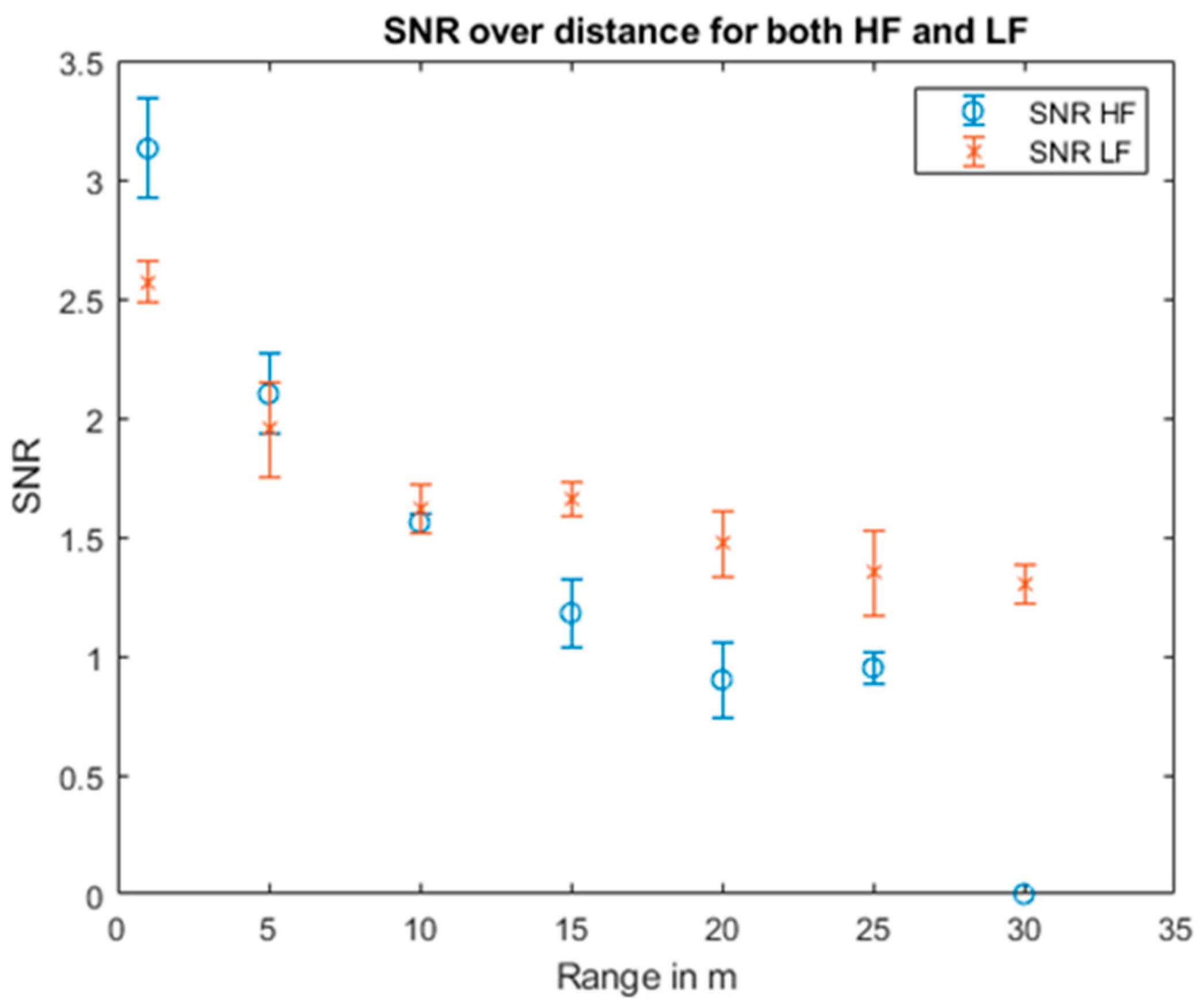
As expected, SNR decreases with increasing range at both high and low frequencies. The difference in SNR between the two frequency modes was greatest at the initial ranges of 1, 5, and 10 m, where SNR was greater for the high-frequency mode. The rate of decline in SNR at high frequency is greater compared to low frequency with both trends shown in Figure 11. Comparing the decline in visibility over range with the results obtained via previous in situ studies with a comparative goal [15,16], a sharp decline in visibility and detectability with range can be seen in both, at similar operating frequencies of 720 kHz (Tritech Gemini 720i and Tritech Gemini 1200ik). Targets were able to be resolved up to 50 m away for the Tritech Gemini 720i while the low-frequency mode of the 1200ik only detected the given target up to 25 m away. However, the target used in this study was static within the water column and did not move, which might have contributed for an increased detection at long ranges. Additionally, the targets used by Trowse et al. [15] had varying strengths as they were made from different materials, making comparisons difficult, which highlights the importance of using a standardised calibration target to allow for sufficient cross-comparisons.

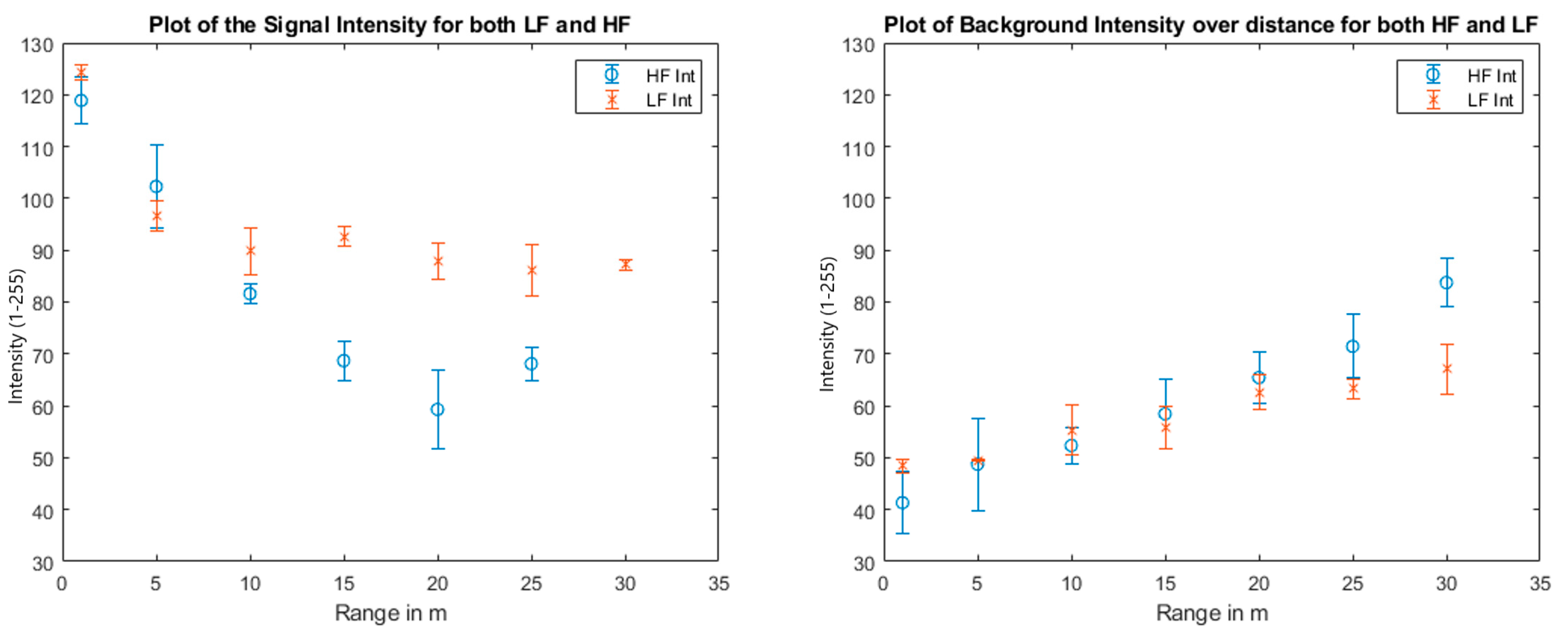
Comparing intensity values between the two modes shows a larger decrease in target intensity at high frequency, reducing the SNR by a factor of 2.18 compared to the low-frequency mode, which shows a reduction by a factor of 1.42. A possible explanation could be the increased effect of absorption, as the higher frequency mode is calculated to have double the absorption over the same range. Additionally, for high frequency, the increase in the background intensity was also greater than the recorded background intensity for low frequency, with a simultaneous drop in the target intensity leading to the greater change in SNR between the two frequency modes. Recorded values at 20 m and 25 m during the high frequency recording had an SNR below 1 showing a higher background noise level than the target, though the target was still visually distinct compared to the background through manual inspection, as the intensity was not spread uniformly [23].

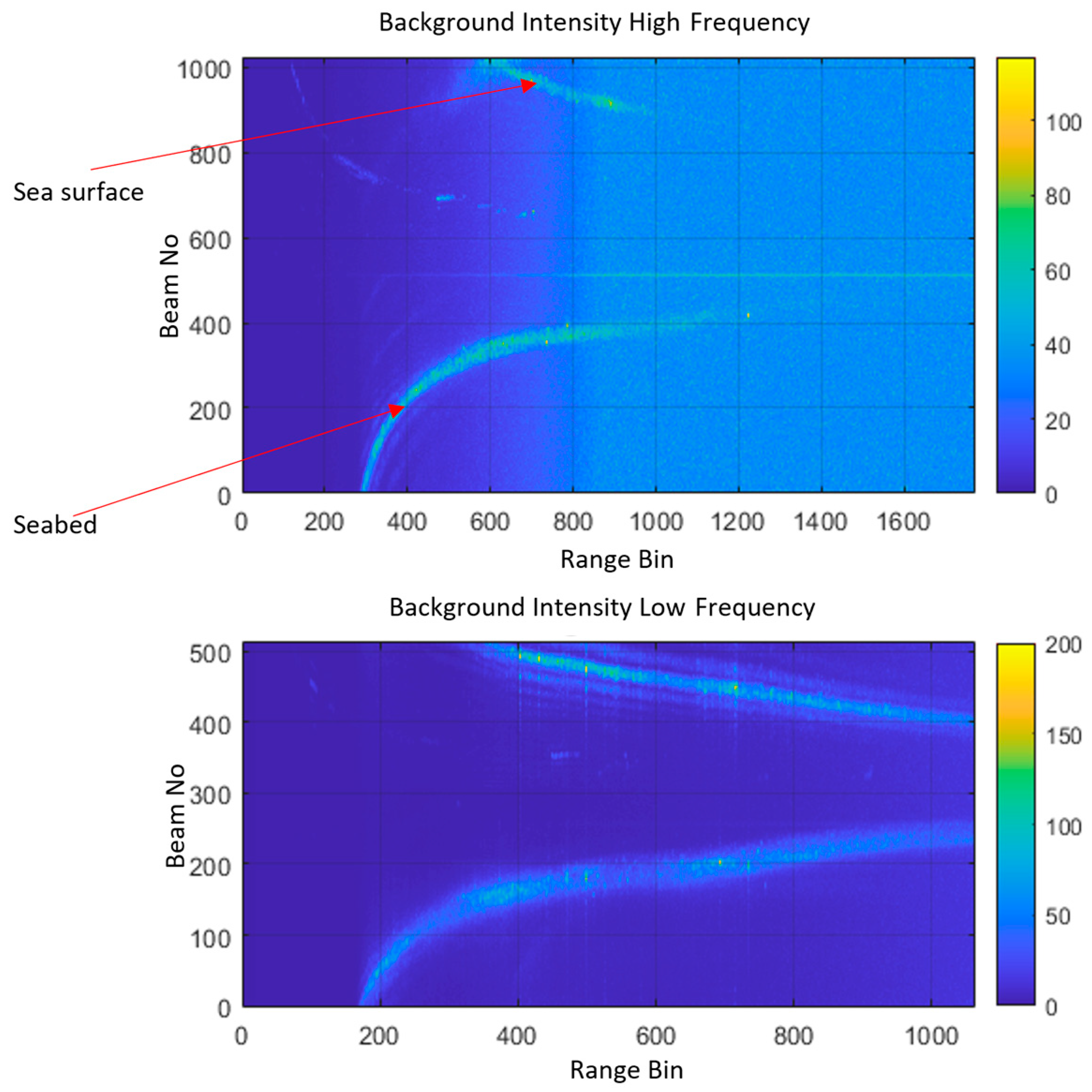
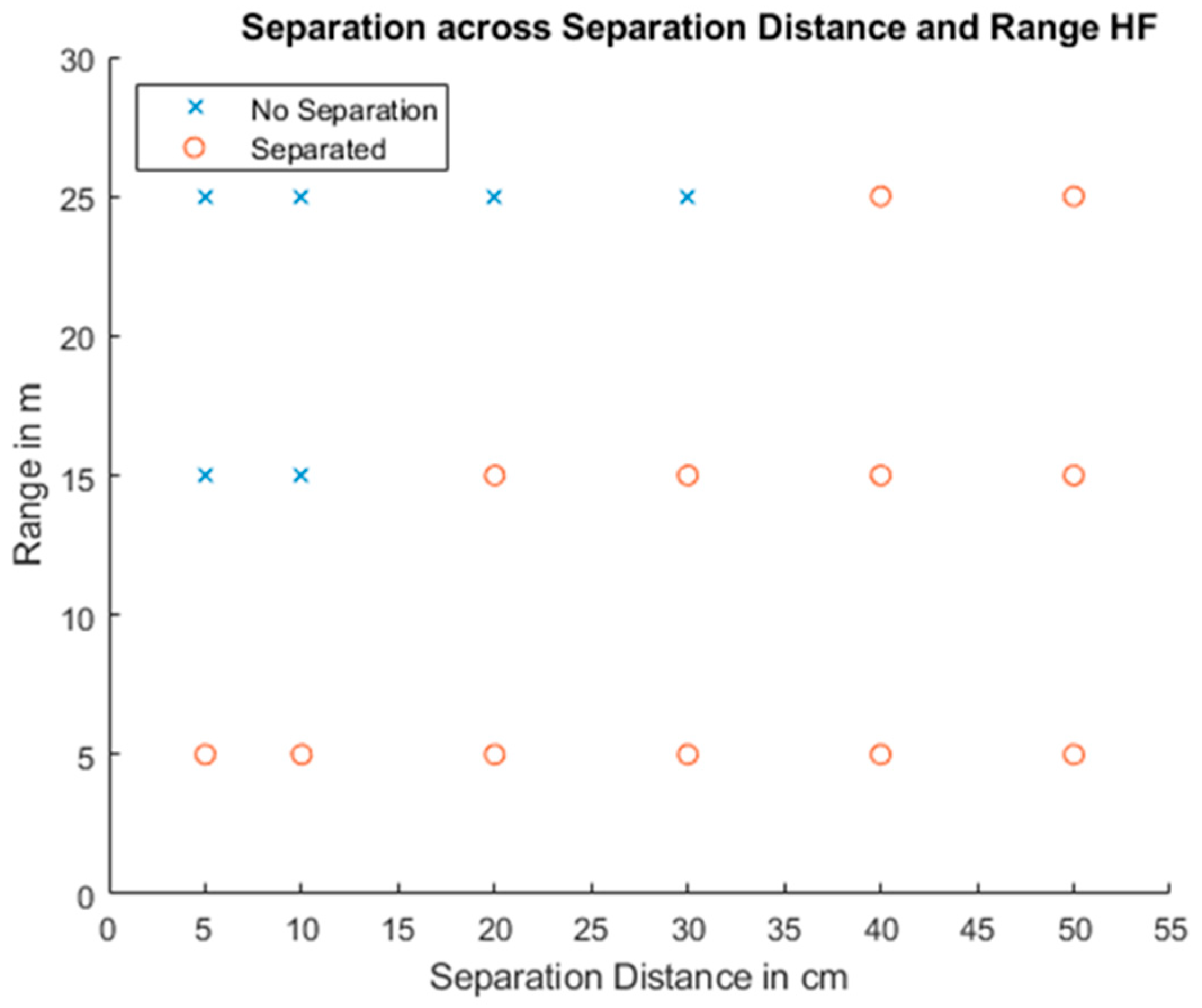
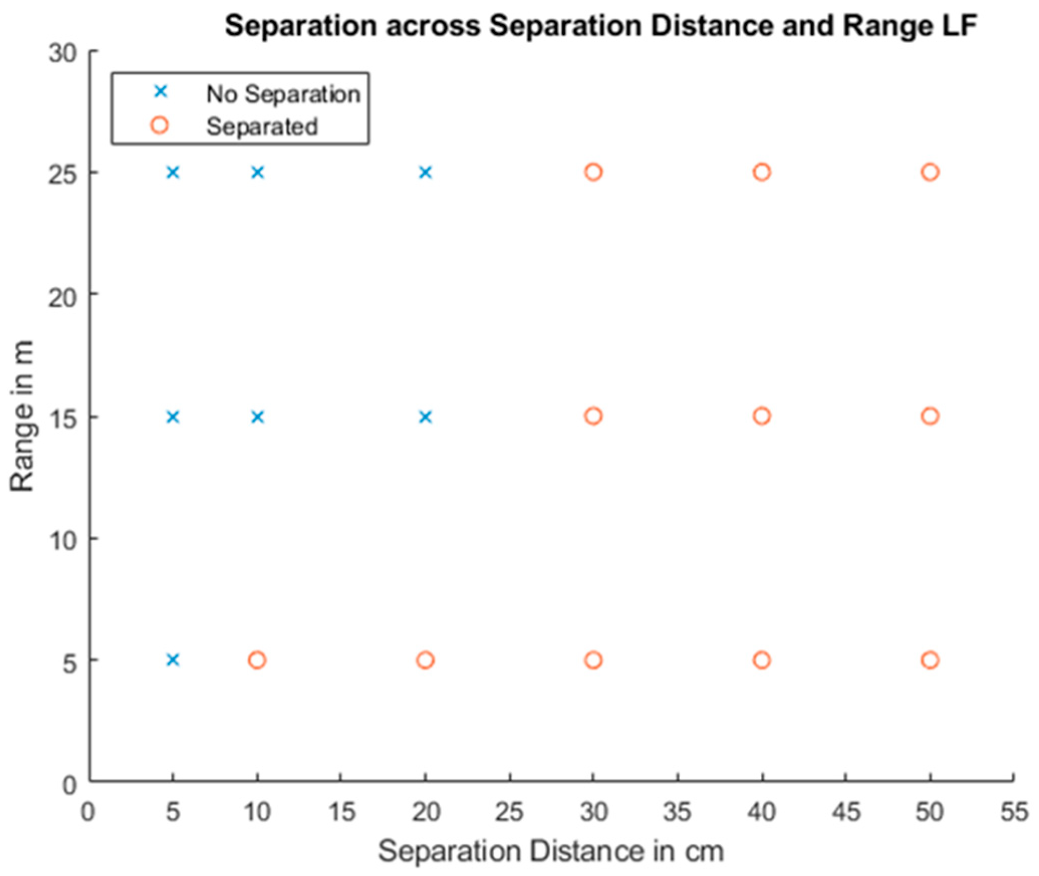
Considering the SNR and separation distance results for high frequency at the 30 m range, it appears that the target is being overshadowed by the background returns and increasing blurred noise from both the sea surface and seafloor. This was also found in the low-frequency data, but to a lower extent, supporting the expectation that the high-frequency mode of the 1200ik will be more affected with noise at higher ranges in the shallow waters of the test site, despite a narrower across-swath beamwidth. Based on the manufacturer specifications, the high-frequency mode is able to operate between the 0.1 and 50 m range, with low frequency being able to work from 0.1 to 120 m. It is assumed that those numbers correspond to deep water tests in a ‘normal’ configuration (120-degree angle orientated horizontally instead of imaging the water column vertically) for a clear water column with a strong reflector as target, though the manual lacks details on the test configuration and target used.

When comparing the trend in SNR and the separation visibility plots, both show a similar trend of high frequency being able to better distinguish targets at short range, while low-frequency mode provides better performance at higher ranges. The main factor is thought to be the higher increase in background noise over increasing range during operation of the high-frequency mode, likely caused by frequency-dependent absorption.

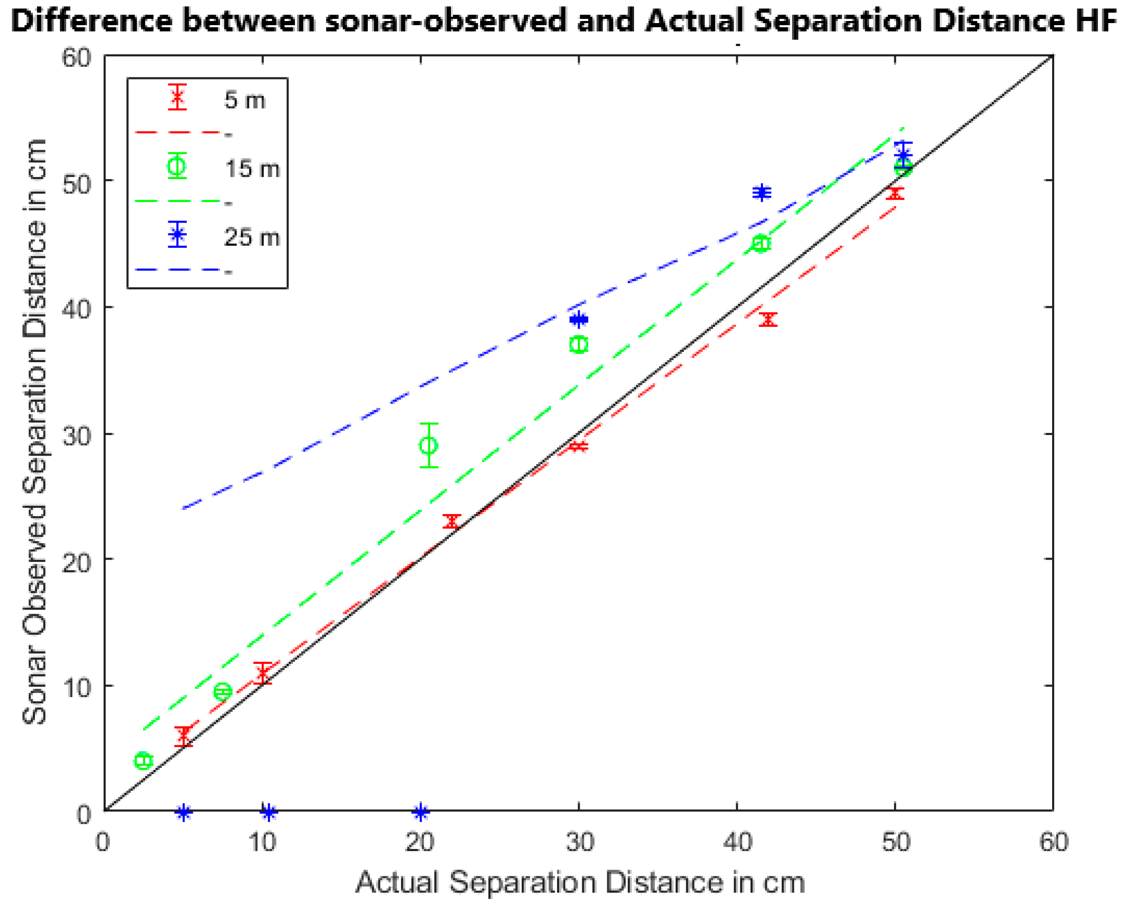
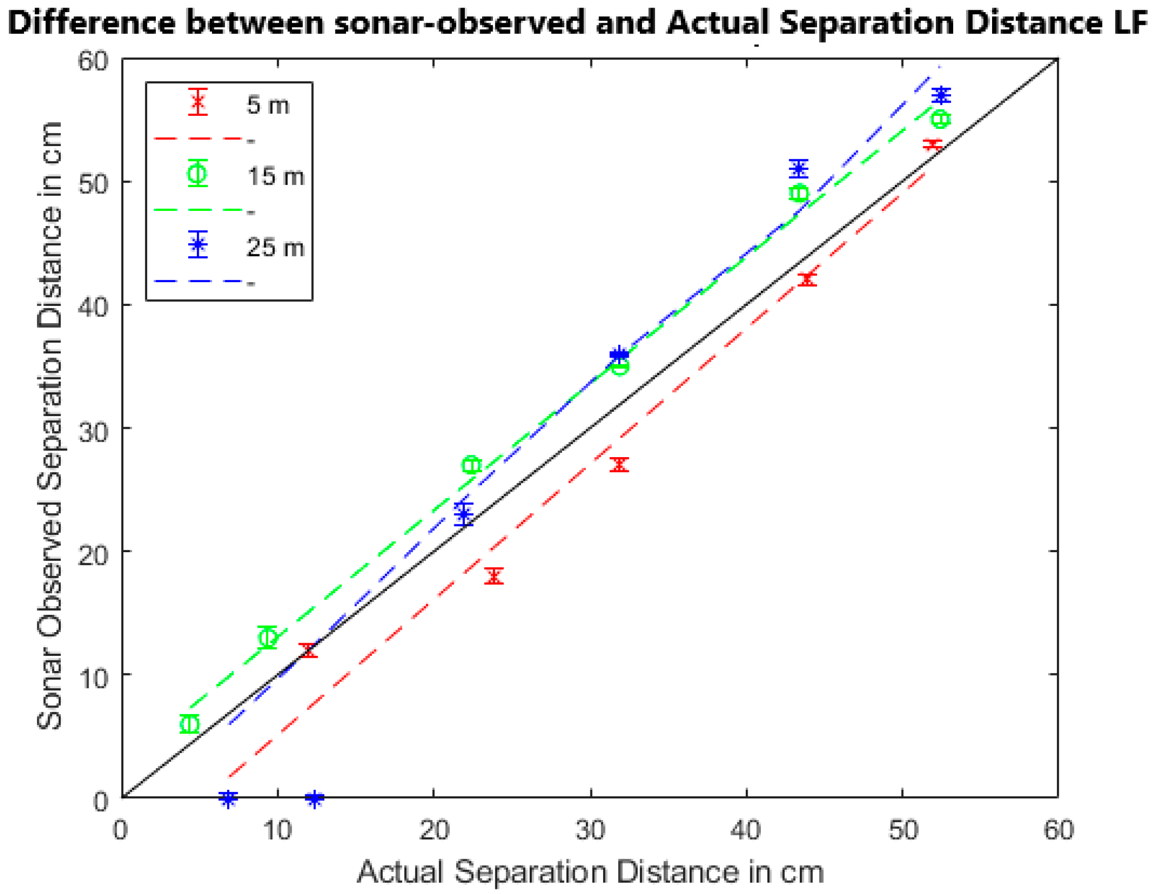
It was determined that, on average, the sonar-observed separation distance increased in both modes with an increase in range, compared to the actual measured target separation. In both frequency recordings at the 5 m range, the actual separation distance was smaller than the sonar-observed separation, which changed at both the 15 and 25 m ranges. In the low-frequency recording, the gradients of the lines of best fit are of a similar value as a one-to-one line, with the lines being shifted in near parallel with a trend of overestimating the sonar-measured distance of separation.

In summary, when target separation can be established (noting a function of frequency mode and range), then the 1200ik provided a generally accurate measure of separation distance with a typical error range of 0.3 cm to 3.5 cm. Comparing the tungsten carbide sphere measurements to in situ measurements of fish length with a high-frequency sonar by Cook et. al. [21] supports the claim that sonar-measured lengths are less accurate. The difference determined by previous studies [21,22] between sonar and baited traps was between ±5 and 20%, which the findings of the present study are consistent with. Previous studies [20,21,22,23] also support the claim of multibeam-generated length measurements, showing an overestimation of target length. Additionally, the range from the multibeam sonar, animal velocity, and angle of imaging can have impacts on the measurements just as they might impact the device capability to detect the target, which could be investigated in future studies of the 1200ik capabilities with biotic targets.

The high-frequency mode shows an on-average higher error in determining separation distance compared to the low-frequency mode, but both show a weak trend of increase in the percentage error with increasing range from the multibeam. At low ranges, the high-frequency mode also underestimated the separation distance between the targets. This may be caused by the shallow nature of the test site, causing reflections of the targets that may have blurred the edges, lowering the intensity gradient between the intensity spikes designated as the centre of the sphere, which shortened the length between the peaks.

4.1. Performance of the Sphere as a Representative Target

The tungsten carbide sphere was chosen as a representative and comparable target based on the extensive previous use for acoustic calibration, documentation about its properties, and to enable the applicability of the results here for comparison with other studies and instruments. The sphere mimics the reflection of an air-filled gas bladder within a fish sufficiently for other studies to be used in calibrating fish returns for single and school targets [13,27,28,29]. Importantly, the target strength does not vary with orientation to avoid biases, such that only position rather than orientation affects the backscattered signal. One of the main assumptions for using a fixed target and comparing it to potential biological targets is that it is representative of the wide variety of potential movements of biotic targets.

When comparing with in situ collected animal data, it should be noted that the target was fixed at a vertical and horizontal distance within the water column to provide a representative and robust test, while potential animal targets can move in and out of the swath and be recorded in opportune positions and orientations that may lessen their backscattered signal.

As the tungsten carbide target is sized at 38.1 mm, this small size also impacts its visibility within an increasing range away from the multibeam. The resolution for the 1200ik is stated as 4 mm (low frequency) and 2.4 mm (high frequency), which will lessen with increasing range settings, which might have affected the visibility of the sphere. As the target chosen for the experiment was a very strong reflector, it can still be assumed that it contributes to the recorded backscatter even when it only occupies a small part of the range and beam bin. Based on the results, it might be said that targets of similar size have a finite range of detection for the 1200ik at low-depth sites; this range was found to be 30 m for the high-frequency mode in these experimental conditions, as the increase in background noise exceeded the backscatter of the strong reflector.

Acoustic backscatter properties of fish are dependent on several factors like signal frequency, species morphology (e.g., swim bladder or not), and their orientation and size as they move through the beam’s swath [13,14,27]. With the 38.1 mm tungsten carbide target representing a potential biotic target with a swim bladder and with a size between 20–30 cm [13], the results show the potential applicability for target detection with the high-frequency mode in shallow waters to moderate distances (25 m). Based on the change in SNR depicted in Table 3, where the SNR flattens out at 1.3 from a range of 25 m onwards, it might be concluded that the target will also be lost within the background noise at the next possible range of 35 or 40 m. Currently, we portray a detection difference between the two frequency modes of 5 m within the shallow conditions of the study site, which is significantly smaller than the proposed 70 m difference between the two operational modes within the 1200ik specification sheet.

The sphere was deemed suitable as a target to estimate the capabilities of detection between the two modes, although future work could consider a suite of different or biological targets.

4.2. Limitations

One of the main factors that could have influenced the results was the method used to determine which frame(s) were used for data processing. It was assumed that for a uniform sphere, the maximum backscatter intensity is achieved when it is acoustically centred within the multibeam across-swath direction. As the multibeam was rotated slowly from left to right over an approximate angle of 30°, it might be that more than one frame exists that shows the potential maximum intensity of the target.

Parts of the high-frequency dataset show the nylon lines that were used to suspend the target spheres. To safely deploy the spheres without causing the sensitive netting to break during recovery, it was decided to use a 0.25 mm line, as the 0.15 mm line broke during a previous trial as the buoy was dragged through the water, although even hints of the 0.15 mm line were observed in the raw data. No alternative suspension techniques were deemed possible or known, and the experiment followed the ICES standard procedure for suspending targets when calibrating acoustic instruments [19,30]. However, in some cases, the lines were visible in possible reflections of the targets (Figure 18).

The low-frequency mode of the 1200ik did not detect the nylon line, making it a high-frequency artefact. Due to taking the maximum intensity over time across all frames to determine the best possible bounding box for the target spheres, an acoustically visible nylon line could interfere with the results of the bounding box, increasing the signal if the nylon reflection coincided with the frame of the maximum target intensity.

It should be noted that most visible nylon lines fell below the cut-off intensity of 75% of the maximum intensity used for the bounding box, with the only exception being at 5 m in the high frequency recording where the intensity of the reflected line approached similar intensity levels as the edge of the target. If there was evidence for a visible nylon line within the chosen frame, the two frames before and after were also analysed and compared against one another to determine the intensity values and bounding box extent, aiming to reduce their possible interference. If an instance was found where the nylon line was encroaching on the bounding box, including the frame before and after, the maximum intensity frame was analysed as described by the methodology, and the bounding box extent and measured intensity within would have been averaged over the frames. This situation did not occur during data processing, but as mentioned at the 5 m range, the maximum intensity of the nylon string approached the 75% cut-off value used for determining the bounding box extent.

Compared to the target bounding box, most visible nylon lines tended to be only one or two pixels wide with a length that tended to be almost double the target bounding box making them very distinguishable from the target (

Table 5. Visualisation showing the maximum intensity and extent (size of an approximate bounding box) of the nylon strings compared to the target.

Range (m)	HF Nylon Size (px)	HF Max Nylon Intensity	HF Target Size (px)	HF Max Target Intensity
5	1 × 14	143	3 × 6	178
10	2 × 8	112	4 × 4	167
15	1 × 12	93	3 × 5	163

) by manual inspection.

Hence, this was deemed to have a negligible effect on the overall experiment which also corresponds to problems and potential issues in previous studies that deal with suspension-based techniques [13,14,19].

5. Conclusions

This field trial provides the first comparative dataset of detection of a standard target across the two different frequency modes of operation and varying ranges using a Tritech Gemini 1200ik dual frequency imaging sonar. It also presented a similar dataset for how the separation between two identical targets is resolved across three ranges. The potential of the 1200ik detection capabilities of a standard target—representing a fish with a swim bladder—within shallow water conditions was observed and discussed. The high-frequency operation mode showed an increased ability for detection and separation at low ranges, with the low-frequency mode allowing for increased detection capabilities at high ranges. Additionally, the visibility of a 0.15 mm and 0.25 mm diameter nylon line at ranges below 5 m further indicated the high sensitivity for target detection with the 1200ik high-frequency mode.

Future investigations will consider target detection across the swath in the 12/20-degree direction. Understanding how target intensity might change while it is not acoustically centred/aligned within the across-swath beamwidth (i.e., 12 or 20°) would provide additional data aiding understanding of the capabilities of the 1200ik and how it can be used to collect animal target data. With the capabilities shown by the high-frequency mode at close ranges, the potential for extending to the analysis of a target shape and size and how those change with range will provide additional characterisation within the field of animal/target classification.

Investigating the feasibility of new instruments also includes the software aspect, which deals with data extraction, processing, and analysis. While this characterisation study mainly used manual techniques to extract targets, other studies have already made efforts to explore the use of automated tools for object detection, extraction, and classification [7,11,30,31]. With the increased amount of data generated with increasing multibeam resolution, the use of automated machine learning tools to accelerate the processing pipeline has increasing potential. The use of bounding boxes for object detection is one of the universal methods in image analysis, followed by the use of spectra analysis via Fourier Transforms. A new method raised by De Curto et al. [32,33] provides the opportunity to employ the Signature Transform to measure similarities in images. Future work in this field could include comparison and evaluation of multibeam imaging sonar data to determine the advantages and disadvantages in different applications.

A different area for investigation might be to investigate the effect of range on observing multiple targets, i.e., fish schools, with a similar method to this study to further understand the multi-target detection and tracking capabilities of the 1200ik. Both future objectives would also supply much-needed ground truth data to test detection capabilities at different conditions and ranges and the capabilities for automated target detection.