
A Numerical Model to Simulate the Transport of Radionuclides in the Western Mediterranean after a Nuclear Accident

1
Department of Física Aplicada I, Universidad de Sevilla, 41013 Sevilla, Spain
2
Department of Matemática Aplicada I, Universidad de Sevilla, 41013 Sevilla, Spain
*
Author to whom correspondence should be addressed.
J. Mar. Sci. Eng. 2023, 11(1), 169; https://doi.org/10.3390/jmse11010169
Submission received: 1 December 2022
/
Revised: 16 December 2022
/
Accepted: 23 December 2022
/
Published: 10 January 2023
(This article belongs to the Special Issue Modeling the Transport of Pollutants and Tracers in the Ocean)
Abstract
:The transport of radionuclides in the western Mediterranean Sea resulting from hypothetical accidents in a coastal nuclear power plant, and in a vessel with nuclear power or transporting radioactive material, was assessed with a Lagrangian model developed for this kind of accident assessment. Water circulation was obtained from the HYCOM global ocean model. The transport model was developed in spherical coordinates and includes advection by currents, three-dimensional turbulent mixing, radioactive decay, and radionuclide interactions between water and seabed sediments. Age calculations are included as well. A dynamic model based on kinetic transfer coefficients was used to describe these interactions. Mixing, decay, and water/sediment interactions were solved applying a stochastic method. Hypothetical accidents occurring at different moments were simulated to investigate seasonal effects in the fate of radionuclides. In addition, simulations for different radionuclides were carried out to investigate the effects of their different geochemical behaviours. Thus, in the case of a coastal release, Cs is transported at long distances from the source, while Pu stays close to the release point due to its strong reactivity, most of it being quickly fixed to the seabed sediment. In deep waters, in case of a surface release, Pu spreads over larger areas since sediments are not reached by radionuclides.
1. Introduction
The recent projects launched by the International Atomic Energy Agency (IAEA), MODARIA, and MODARIA-II [1] have highlighted the need to have numerical models of radionuclide transport in the marine environment ready to run in areas which could be potentially affected by a nuclear accident, in order to be able to carry out a quick assessment of the accident aftermaths. These accidents could be a radionuclide release from a nuclear facility, such as in the Fukushima Daiichi case in Japan, or due to an accident in a ship transporting nuclear waste, or equipped with nuclear power, for instance.
Thus, some recent works have focused on developing radionuclide transport models for several marine areas of the Earth which could be affected by a nuclear accident. These are the cases of the Red Sea [2], the northern Indian Ocean [3], the Arabian/Persian Gulf [4,5], or the eastern Mediterranean Sea [6].
The purpose of the present work consists of describing a radionuclide transport model for the western Mediterranean Sea. Some nuclear power plants operate on the coast of Spain. In addition, the Rhone River in France receives radionuclides from the Marcoule nuclear complex; thus, this river could be a source of radionuclides into the sea in case of an accident in this complex. The transit of nuclear-powered vessels, mainly military, and thus some of them carrying nuclear weapons, must be considered as well. As a consequence, it is pertinent to have an available transport model for this region, as stated in the frame of IAEA projects [1].
The model is Lagrangian in nature. Thus, the radionuclide release is simulated by a number of particles, each one equivalent to a number of Bq, whose trajectories are calculated during the simulation. The model includes advection by currents, three-dimensional turbulent mixing, radioactive decay, and uptake/release of radionuclides between water and seabed sediments. A novel feature, with respect to works cited above, is that it is formulated in spherical coordinates. Its description is summarized in Section 2 and some application examples are presented in Section 3.
2. The Model
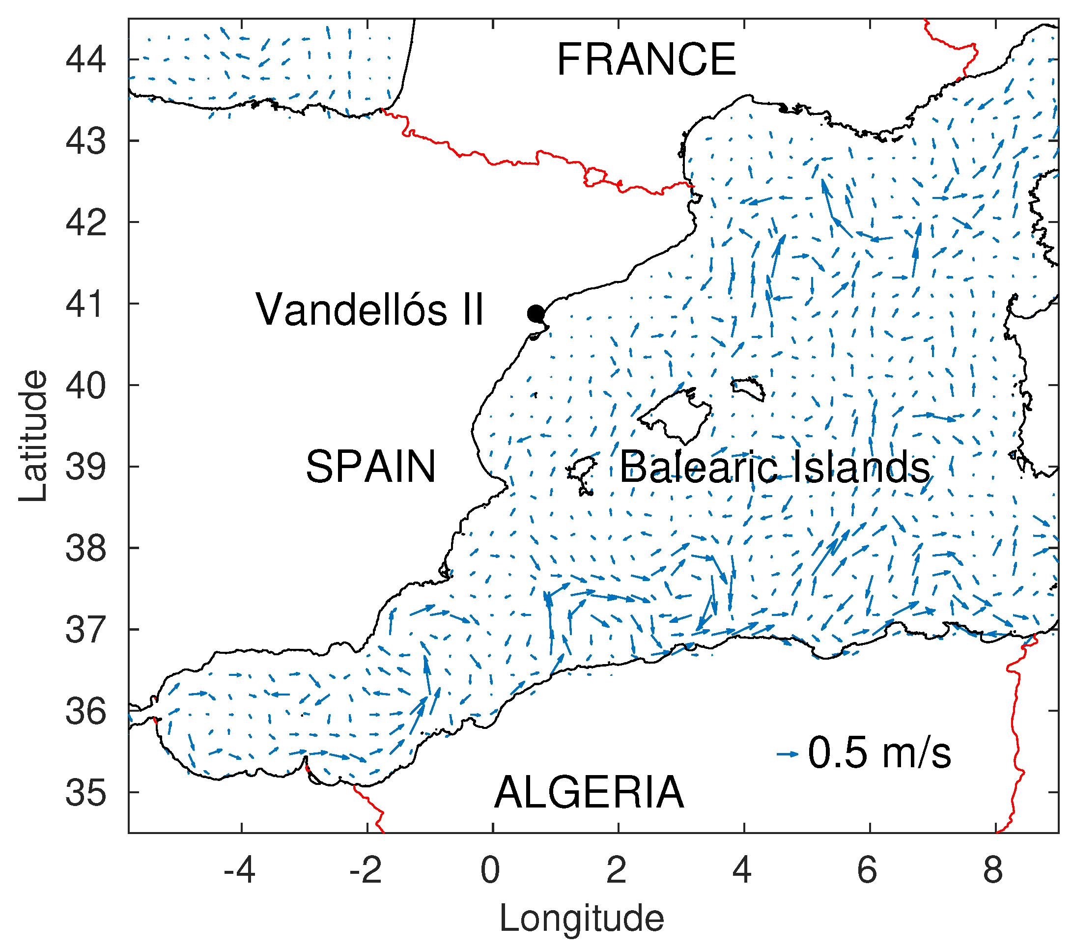
As commented before, the model is Lagrangian, and thus the radionuclide release is simulated by a number of particles whose trajectories are calculated during the simulated period. Advection is the transport due to water currents. Consequently, the water circulation must be known in the area of interest. The model domain extends from −5.80° to 9.00° in longitude and from 34.50° to 44.50° in latitude. The water currents over this domain were obtained from the HYCOM global ocean model [7]. It is forced by results from atmospheric modeling, which provides winds, short– and long–wave radiation, freshwater inflow through the main rivers and precipitation, air temperature, specific humidity, dew point, and atmospheric pressure. Many application examples can be seen on the model web page (https://www.hycom.org/, accessed on 1 July 2022), and some particular applications to the Mediterranean Sea can be seen in [8,9]. The model consists of 32 vertical levels and its horizontal resolution is 0.08° in longitude. However, horizontal resolution in latitude is not uniform (ranging between 0.0659° and 0.0571°), and consequently it was more appropriate to operate in spherical coordinates. Cartesian coordinates were used in the works cited above [2,3,4,5] since in these cases the horizontal spacing was uniform in the corresponding HYCOM model runs. Tides are not included in the HYCOM model, but they are weak in the Mediterranean Sea and thus can be neglected [10]. As an example, the model domain showing surface circulation for 31 January, as downloaded from HYCOM, can be seen in Figure 1.
If u and v are the horizontal currents (in west–east and south–north directions, respectively) downloaded from the HYCOM ocean model, then the corresponding changes in longitude, , and latitude, , of a given particle during a time are as follows:
where is the radius of the Earth, is the present latitude of the particle, and is the time step used to integrate the model.
As usual [2,3,4,5,11], the horizontal step given by a particle due to turbulent mixing is
in the direction , where is a horizontal diffusion coefficient and s are independent random numbers between 0 and 1. Therefore, the corresponding changes in the longitude and latitude of the particle, due to mixing, are
Equations (1), (2), (4), and (5) give the changes in longitude and latitude in radians. They must be multiplied by to convert them to degrees.
A constant value m/s is used for the horizontal diffusivity, which is appropriate for the present grid resolution [4,5]. More complex schemes, such as the Smagorinsky one [12], can be used, but this scheme very significantly increases the computing time [3], which is not appropriate for a rapid assessment after a nuclear accident. A constant diffusivity was used in other models of semienclosed seas [2,4] as a good compromise with computation speed.
The size of the vertical jump given by the particle because of turbulent mixing is [2,3,4,5,11]:
where is a vertical diffusion coefficient. This jump may be given either towards the surface or the sea bottom. A new independent uniform random number is generated and used to decide the jump direction through the following equation:
where is the vertical displacement of the particle, measured downwards from the sea surface. The vertical diffusion coefficient is considered to change with depth according to the following:
where z is water depth below the surface. The increased turbulence in the mixed layer of the ocean is described in this way. In addition, the turbulence is smaller in the pycnocline and deep sea. This description was used in models applied to simulate Fukushima releases in the Pacific Ocean [13] and also in a radionuclide transport model in the Indian Ocean [3]. The mixed layer depth in the western Mediterranean Sea shows seasonal variability, ranging from about 10 to 100 m [14]. A mean representative value of 50 m was used in this model to distinguish between surface and deep water layers. Of course, the use of a constant mixed layer thickness is an approximation to speed up calculations.
Radioactive decay is calculated using a stochastic method [11]. If is the radioactive decay constant of the considered radionuclide, then the probability that a given particle decays during a time step is
A new independent random number is generated. If it is smaller than , the particle is considered to decay and therefore it is removed from the computation.
The radionuclide interactions between water and sediments are described using a 1-step kinetic model [15] consisting of a single reversible reaction. Thus, the adsorption and release reactions are governed by the corresponding kinetic rates and . A stochastic method is used again to solve these processes. The probability that a dissolved particle is adsorbed by the sediment is defined as follows:
If a new generated independent random number is , the particle is fixed to the sediment. It is considered that only particles which are at a distance from the seabed smaller than m can interact with it.
Similarly, the probability that a particle which is fixed to the sediment is redissolved is defined as follows:
and the same procedure as above is used. is a correction factor that takes into account that part of the surface of sediments is hidden by the surrounding sediments. Consequently, the hidden part cannot interact with water. Full details of this procedure may be seen, for instance, in [2,3,4,5,11]. The concentrations (in Bq/m) of radionuclides in the 50 m thick surface mixed water layer are calculated, counting the number of dissolved particles per grid cell. The same procedure applies for particles fixed to the sediment (concentrations in Bq/m in this case). The procedure is explained in detail in [5], for instance. The correction factor was fixed as as in other works [4,16,17,18].
The adsorption rate is obtained from the desorption coefficient and the radionuclide distribution coefficient for coastal waters (full details may be seen in [15]). As described in this reference, the is the ratio between radionuclide concentrations in sediment and water once equilibrium in the partition has been reached, and then it is written as follows:
where m is the sediment concentration. In this case, m must be understood as the mass of seabed sediment in a grid cell divided by the water volume which can interact with it. In Equation (12), the is given in m/kg, m in kg/m, and the kinetic rates are measured in s.
The seabed sediment concentration m in the water layer of thickness H which interacts with the sea bottom is (see, for instance [19]) as follows:
where L is the thickness of the sediment layer which interacts with water and is the bulk density (dry weight divided by wet volume) of the sediment. Bulk density is calculated as , where is the density of mineral particles and p is sediment porosity.
Then, the equation used for is
where is a correction factor, as explained above (Equation (11)).
If typical values (such as in models in [2,3,4,5,20,21]) are used: m, kg/m, and , and the water layer interacting with sediments is m, as mentioned above, then a value of kg/m results.
recommended values for coastal waters were compiled by the IAEA [22]. The value of the desorption rate was obtained from the experiments in Nyffeler et al. [23], s. It was used in many previous modeling works involving different radionuclides (see, for instance, the review in Periáñez et al. [20]).
The ages of particles released to sea are also calculated with the model, since they can provide useful oceanographic information and their calculations do not demand significant computational resources. Age is defined as the time elapsed since a particle was released into the sea. It is a Lagrangian concept, calculated by attaching a clock to each particle, which starts at the time the particle is released. According to the age-averaging hypothesis of Deleersnijder et al. [24], the mean age of particles within each grid cell is defined as the mass-weighted arithmetic average of the ages of the particles present there. The mass of a given Lagrangian particle i is defined as its radioactivity content . Thus the mean age, , in a given grid cell is
where N is the number of particles within the cell and is the age of particle i. If were the same for all particles, then the mean age is just the arithmetic mean of the clock readings:
For a given simulation, the following information must be provided to the model: release location (geographical coordinates) and depth; release date; release duration; release magnitude; simulation time; radionuclide decay constant; and . The model can deal with instantaneous releases or releases lasting any time. Output files (radionuclide concentrations in the mixed water layer and sediments, and ages of radionuclides in the mixed layer, deep water, and sediments) are generated at the end of the simulated time.
The time step used to integrate the model is s. Stability conditions imposed by the terms describing water/sediment interactions are satisfied with this value [25]:
where is the maximum kinetic rate involved in the model. In addition, it is ensured that the spatial displacement given by a particle during due to advection and diffusion is not larger than a grid cell size, which is a condition required in Lagrangian models [11].
The number of particles used in the simulations presented in this paper is , although it can be changed. With this number of particles and for a 90-day-long simulation, running times range from 15 min, in the case of a 90-day continuous release, to 45 min, if the release is instantaneous.
3. Results
Several hypothetical accidents occurring in the Vandellós II nuclear power plant (NPP) were simulated. This NPP is located on the east Spanish coast, at coordinates 40°57′ N 0°52′ E (see the location in Figure 1). It started its operation in 1988 and consists of a pressurized water reactor with 1087 MW power. The purpose of these simulations is to show some examples of model performances, and also to show how some information on the transport pathways of radionuclides may be inferred from the calculated ages, but the model can, of course, be used as a rapid-response tool to support decision-making after a radioactive release occurring anywhere in the western Mediterranean at any temporal scale. Although a number of radionuclides are released in the case of a nuclear accident, Cs and Pu were chosen as examples of radionuclides with very different geochemical behaviours. As mentioned above, only the radionuclide , decay constant, and release data must be modified to deal with different radionuclides.
It must be mentioned that comparisons between model results measurements are not possible since hypothetical accidents were simulated. Nevertheless, the methodology presented in this work has been tested in model intercomparisons carried out in the frame of IAEA exercises [1] and applied to real situations in which comparisons of model results with measurements in water and sediment could be carried out. As examples, Fukushima releases in the Pacific Ocean [13,26], releases from European nuclear fuel reprocessing plants in the Atlantic Ocean [17,27], and Chernobyl deposition on the Baltic Sea [28] can be mentioned.
Several releases of Cs were first simulated. All releases occur in dissolved form. The release was supposed to occur at the surface, with magnitude 1 PBq and lasting 90 days. It was considered uniform in time. This is an example of the same order of magnitude as the direct releases of Cs from Fukushima NPP into the Pacific Ocean during the first three months after the tsunami in 2011 [29]. Four hypothetical accidents were analyzed, starting on 21 March, 21 June, 21 September, and 21 December, in order to observe any potential seasonal effects in transport pathways. Radionuclides are directly released into the sea. However, atmospheric releases often occur in the case of a nuclear accident. These radionuclides are later deposited on the sea surface, as occurred in the case of the Fukushima accident [13,29,30]. An example of deposition of Cs on the Mediterranean Sea was the Acerinox incident that occurred in May 1998 in the south of Spain: a Cs source passed through the monitoring equipment in the Acerinox scrap metal reprocessing plant. When melted, a radioactive cloud was detected in several countries in Europe. Part of the radionuclides were deposited on the Mediterranean Sea surface, and their transport was simulated by means of a box model [31]. Although the present model can treat this atmospheric deposition, only direct release examples are presented.
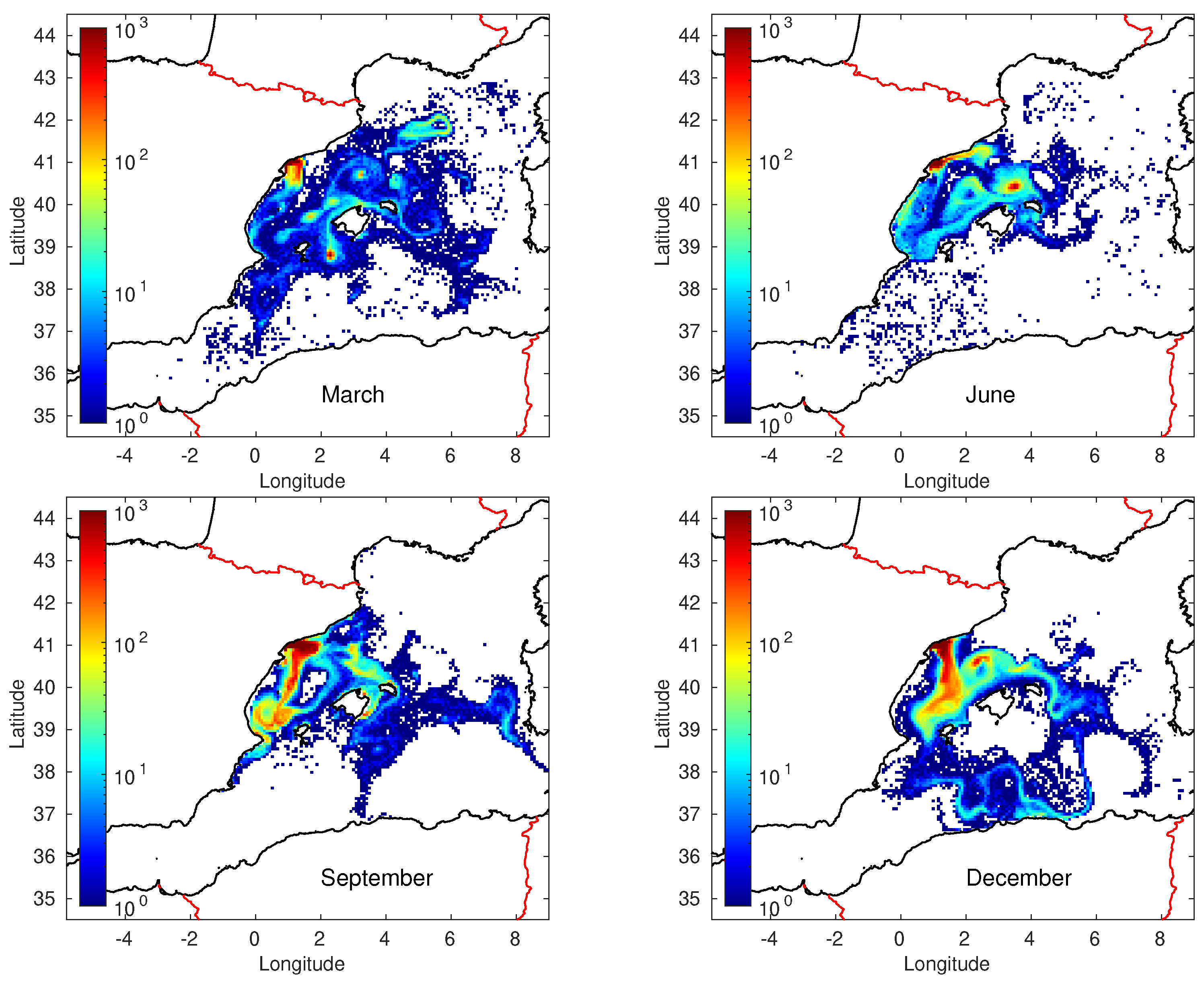
The calculated concentrations of Cs in surface waters for the four accidents can be seen in Figure 2, and the corresponding ages of these radionuclides in Figure 3. The extension of the radionuclide patch is different for each experiment. If the accident starts in March, radionuclides travel to larger distances from the source, extending over a greater region of the western Mediterranean. In June, some radionuclides reach the African coast. This also occurs in the June and September accidents, although a shorter length of the coast is affected by the releases in the September case. The Balearic Islands are affected by the releases in all cases, although it may be noted that radionuclides do not arrive on their south coasts if the accident starts in September. In all cases, concentrations of Cs in surface water arising from an accident similar to that of Fukushima would be significantly higher than measured background in the Mediterranean Sea surface, which is about 1.5 Bq/m (decay-corrected to present date; measurements carried out in 1995) [32].
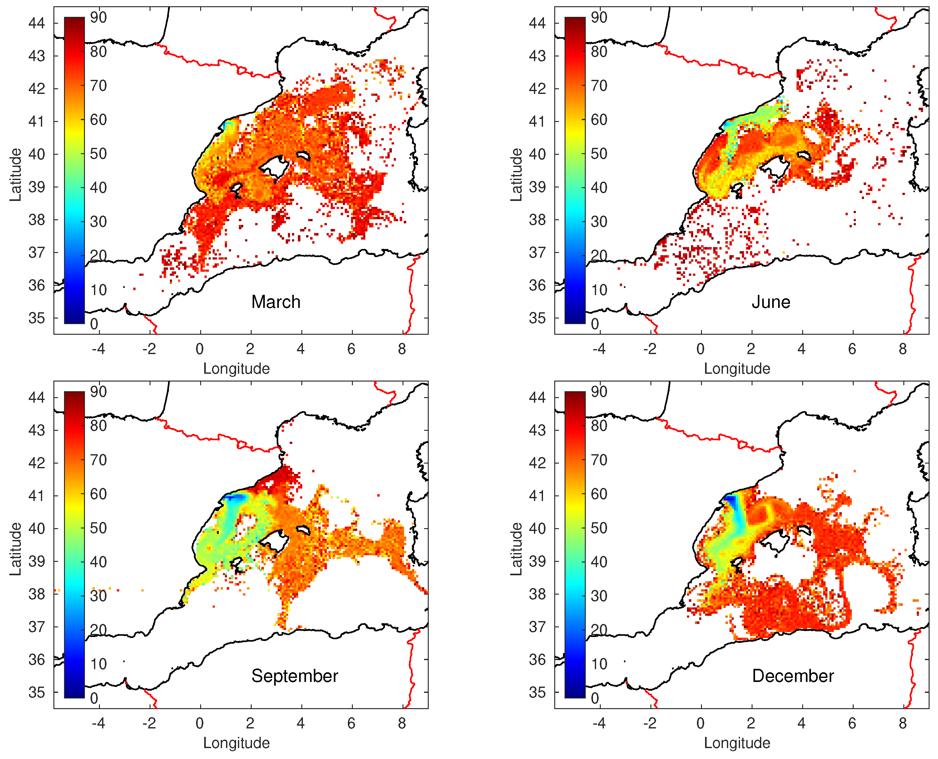
The age distributions in Figure 3 help to visualize the transport pathways. Of course, the extension of the colored map is the same as in Figure 2 since age is zero in grid cells where there are not radionuclides. It must be taken into account, however, that age distributions do not represent a snapshot of water circulation at a given time since the release lasts three months. As a consequence, these age distributions are an integration of circulation during these three months. For accidents starting in March and December, it can be seen that the most recently released radionuclides (blue–green colors) traveled to the south. Older discharges (orange–red) traveled around the Balearic Island in a rather symmetric form. In the case of the accident starting in September, it can be appreciated that the integrated circulation in the period is cyclonic around the Balearic Islands: the older radionuclides are close to the northwest coast of Spain and there is gradual transition to younger ages around the Balearic Islands. The most recent radionuclides also traveled to the south from the source, as in previous cases. If the accident starts in June, some old radionuclides return close to the south of the release area, although old radionuclides are also present to the east and northeast of the Balearic Islands as well as close to the African coast. In addition, there is a transition in the circulation in the release area from southwards to northwards in the last stages of the accident.
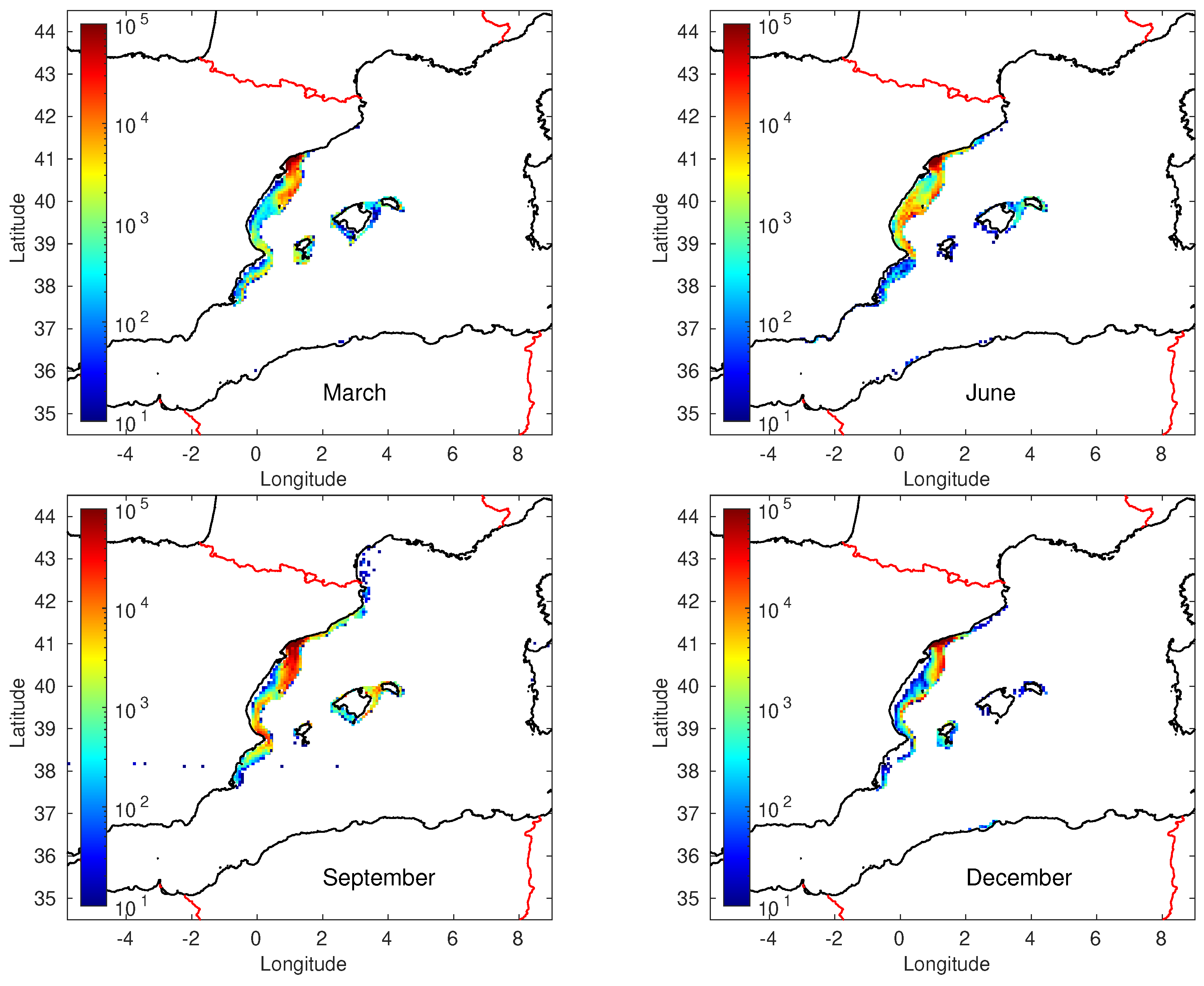
The calculated Cs concentrations in bed sediments for the four accidents are presented in Figure 4. Background levels in the Mediterranean Sea sediments are ∼10 Bq/kg [33], which are about 500 Bq/m with the values for L, , and p used in this work. A band of contaminated sediments along the Spanish coast is apparent in all cases, with concentrations some orders of magnitude above background. Radionuclides do not reach the seabed as water depth increases, and sediments are again contaminated in the shallower areas around the Balearic Islands, although with concentrations significantly above background mainly in the September accident. In the December simulation, a smaller quantity of radionuclides reach these islands. Sediments of the southeastern coast of France are also reached by radionuclides in the simulation carried out for September, although with low concentrations (below background levels).
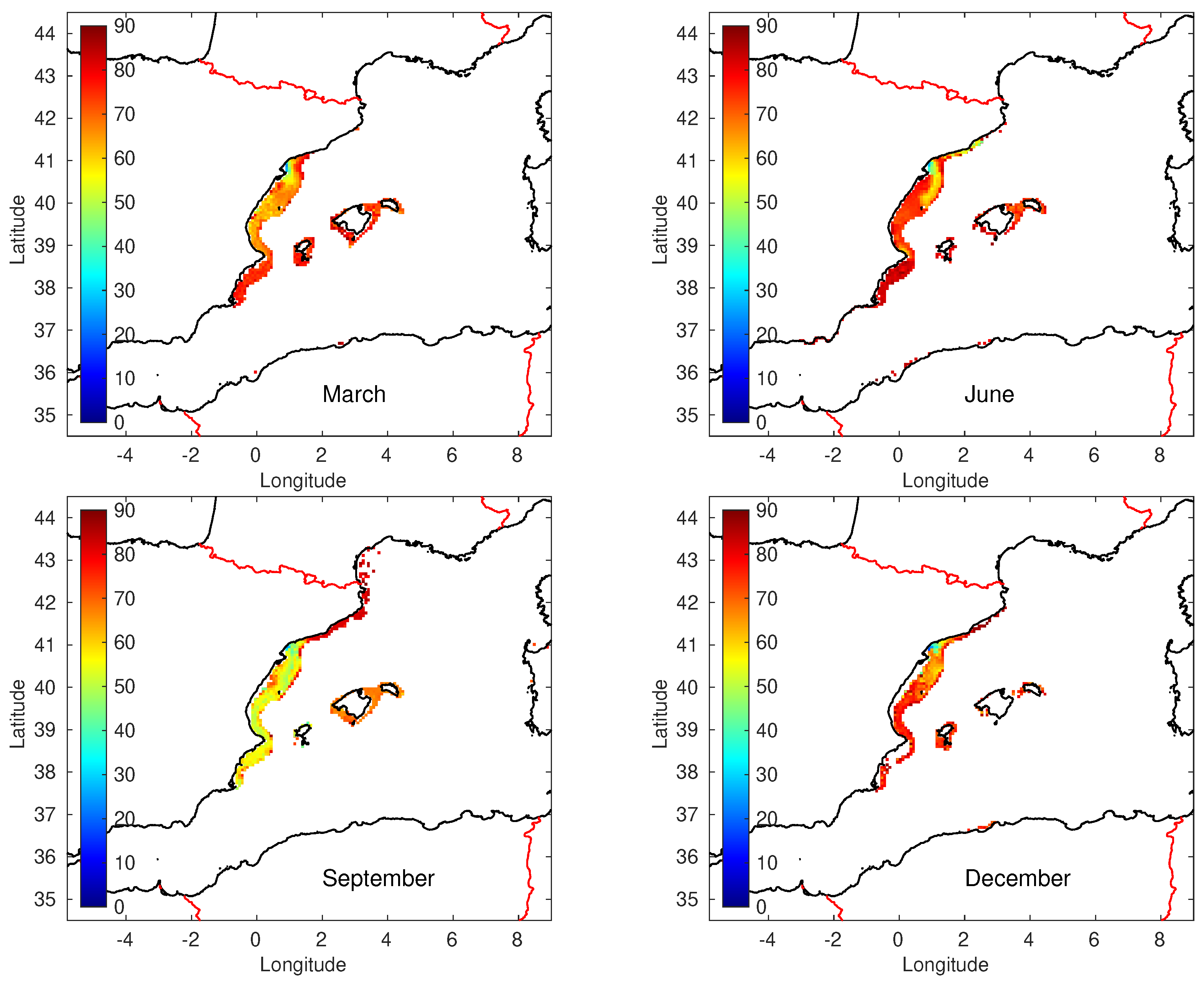
The age distributions of radionuclides in bed sediments (Figure 5) indicate that the Balearic Islands are reached by radionuclides soon after the releases occurring either in March or in June (red colors around the islands, thus oldest radionuclides). However, about one month is required in the case of the September accident (age is about two months). In addition, in this just-mentioned accident, it can be seen that radionuclides initially traveled northwards along the Spanish coast, and after about one month the coastal circulation reversed to southwards. Similar changes in circulation are apparent for the March and December accidents, although they occurred soon after the accident starting time.
The same accidents were simulated in the case of plutonium using a typical total release of 1 TBq, as explained below. Results (not shown) are completely different due to the extreme low mobility of this element in the marine environment. Since the release occurs from a coastal facility, thus in shallow waters, plutonium is quickly fixed to bed sediments of the release area. Actually, radionuclides in sediments are not given by the model at distances longer than a few tens of km from the release point. This is, for instance, the case with measurements of Pu off the shore ofFukushima [34]: results did not show contamination due to the accident more than 30 km away fromthe power plant. This effect was also observed in Pu simulations for this accident [21].
There are other scenarios, besides an accident at a coastal nuclear power plant, in which a radionuclide release could occur. For instance, in 1966, a US B-52 bomber collided with a refueling airplane near the village of Palomares in southeast Spain. As a result, two of the four thermonuclear weapons carried by the B-52 were destroyed, and plutonium contaminated about 2.5 km of soil. This plutonium was later washed into the Mediterranean Sea by rains. The total input to the sea was estimated at 1.37 TBq of Pu + Pu [35]. Another B-52 crashed on ice near Thule (Greenland) in 1968. As a consequence of the accident, the marine environment was contaminated (mainly bed sediments) with a Pu inventory estimated at 3.1 TBq [36].
Other accidents have occurred in nuclear-powered ships and/or ships carrying nuclear weapons. For instance, the nuclear-powered submarine Komsomolet sank in the Norwegian Sea in 1989 with about 16 TBq of Pu in two nuclear weapons and 5 TBq of actinides in the reactor core. Fortunately, only a minor contamination resulted from the accident [37]. In some cases, accidental releases have occurred at military bases during maintenance works of military and civilian nuclear-powered vessels. An example of the last is the accidental release from the icebreaker Lenin into the Kara Sea that occurred in 1965 [38].
In this work, an accidental release of Pu from an accident of this kind was supposed to occur far from the coast, at coordinates 1.5° E, 37.8° N. This point is located between the Balearic Islands and Algeria, and water depth here is 3000 m. A typical representative release of 1 TBq of Pu (see paragraphs above), instantaneously occurring, was considered. Thus, this example is also useful to see the model performance in instantaneous releases. Three release scenarios were studied: surface, mid-depth, and seabed releases (for instance, due to a sunk vessel). For each of these three cases, the same four accidents as before were considered, occurring on 21 March, 21 June, 21 September, and 21 December, to see any potential seasonal effects in transport pathways. Simulation time was 90 days, as before, in all cases.
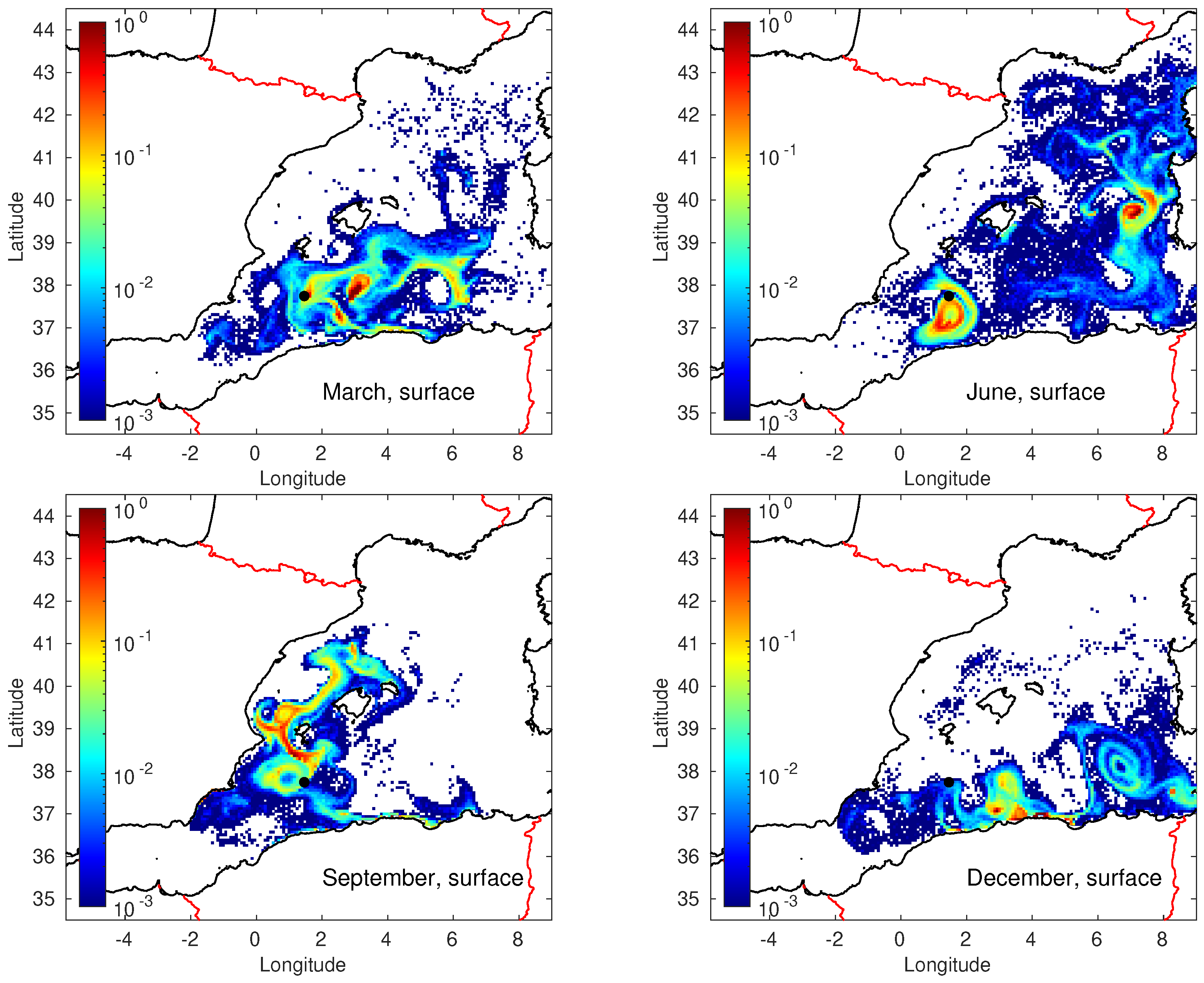
The calculated Pu concentrations in surface water, for the release occurring on the sea surface, are presented in Figure 6. The behavior of the patch clearly depends on the moment of the year when the accident took place. For instance, in December and September, most of the radionuclides are, after 90 days, located, respectively, in the southern and western regions of the domain. In contrast, most of the western Mediterranean is affected if the accident occurs in June. In all cases, a number of gyres and meanders with higher concentrations than in surrounding waters can be appreciated.
Measured Pu concentrations in the surface waters off Monaco (northwestern Mediterranean) are on the order of Bq/m [39]. Thus, this accident would lead to concentrations higher than those measured in Mediterranean waters in significant parts of the sea. These enhanced concentrations would also reach the coast on some occasions, for instance, the Algerian coast in the March, September, and December accidents, and a small fraction of the Spanish coast in the September accident.
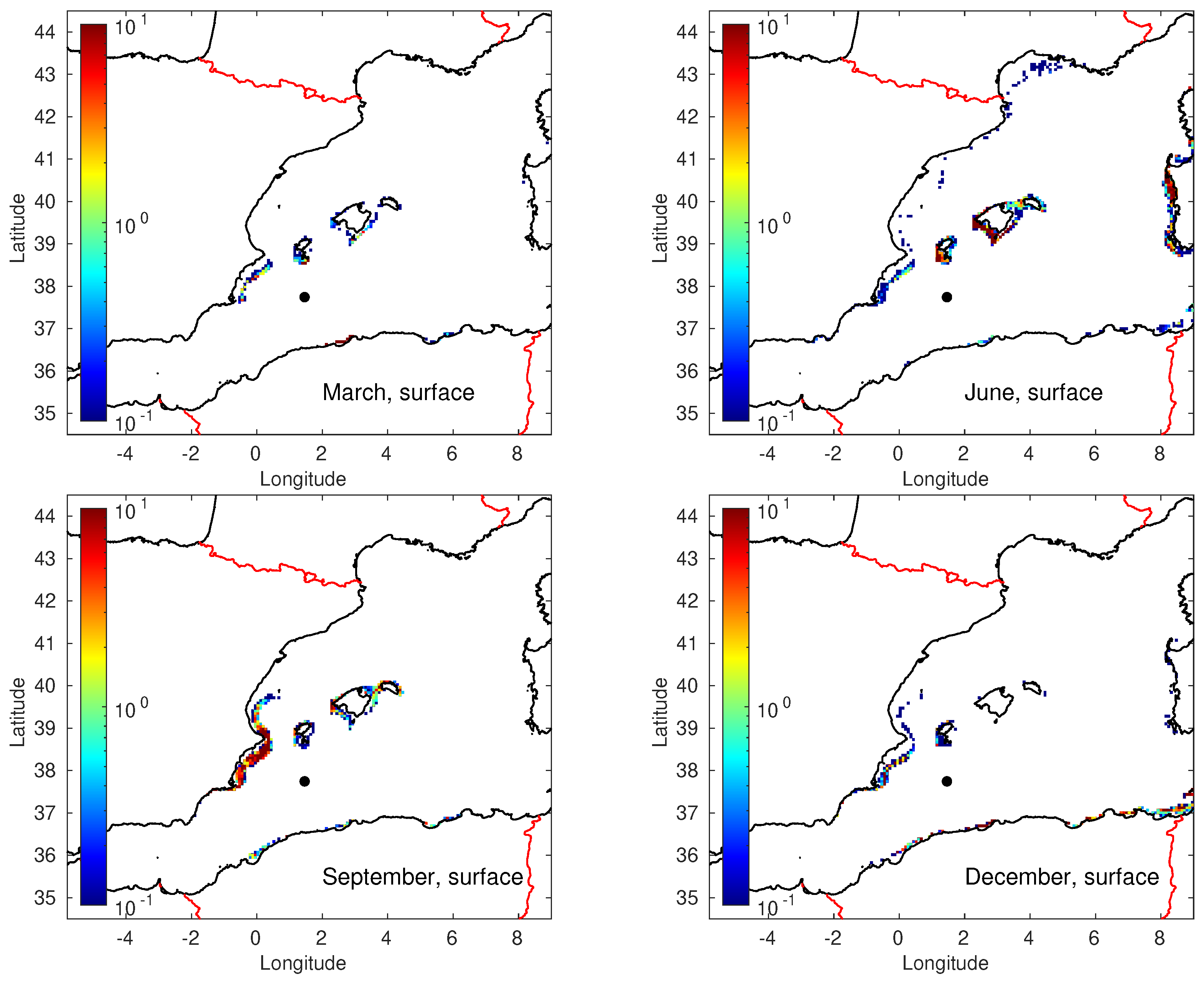
The resulting concentrations in bed sediments for the sea surface releases can be seen in Figure 7. The sediments are affected by the releases in the coastal regions, i.e., when waters are shallow enough to allow radionuclide interactions with the seabed. The eastern Spanish coast, for instance, is more affected if the accident occurs in September, and the Balearic Islands is more affected if it takes place in June, reflecting the radionuclide distributions in surface waters (Figure 6). Sediments in the area off Monaco present Pu concentrations on the order of 1 Bq/kg [40], i.e., approximately 50 Bq/m. Thus, the resulting Pu concentrations in sediments due to the simulated accidents would not be significant, being on the order, or below, of those measured.
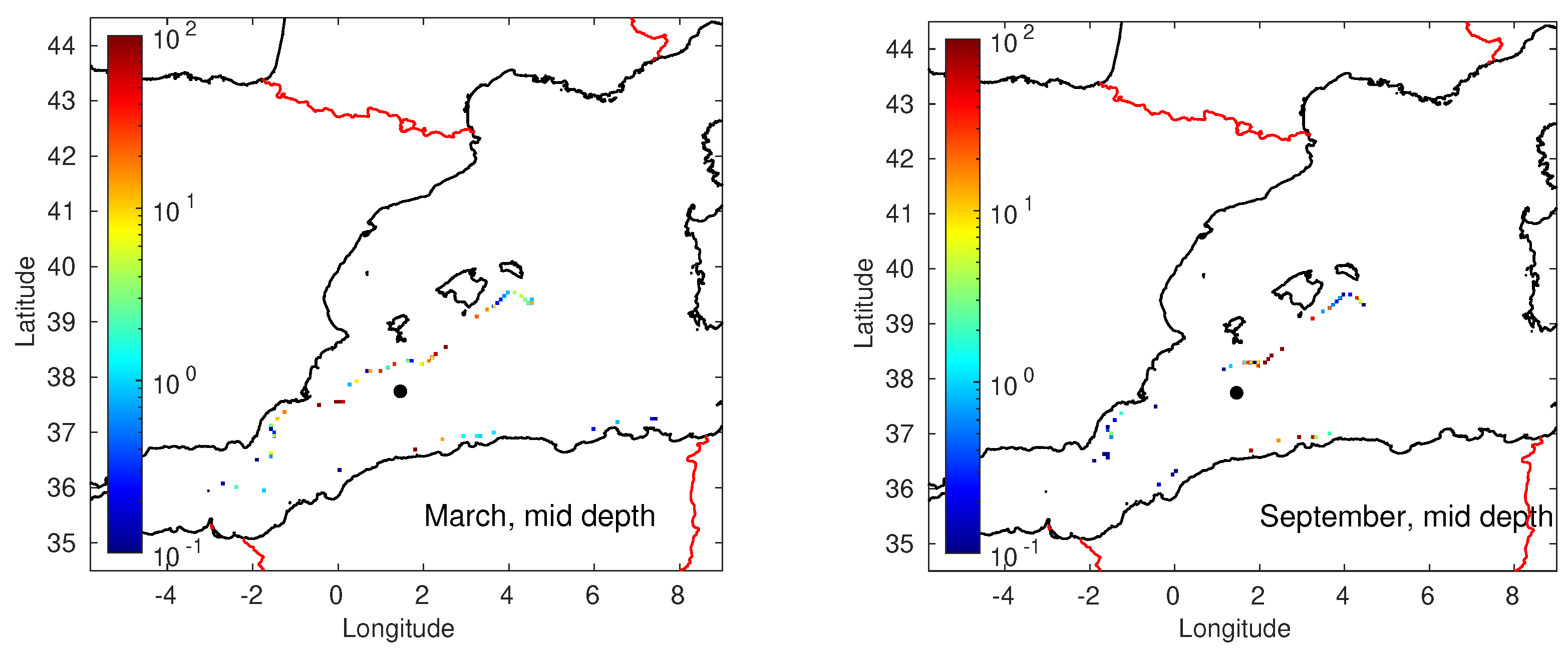
If the release occurs at mid-depth of the water column (1500 m) or close to the seabed (2990 m), radionuclides do not reach the surface water layer in any case. The resulting Pu concentrations in bed sediments for the mid-depth release are presented in Figure 8 for the March and September accidents. Both distributions are very similar, and the same happens in the cases of the June and December accidents (not shown). It can be concluded, therefore, that seasonality does not influence the results in these cases. Sediments of the 1500 m isobath are contaminated when water containing traces of Pureaches them. Nevertheless, peak concentrations are about one order of magnitude higher than if the release occurs at the sea surface (compare the color scales in Figure 7 and Figure 8).
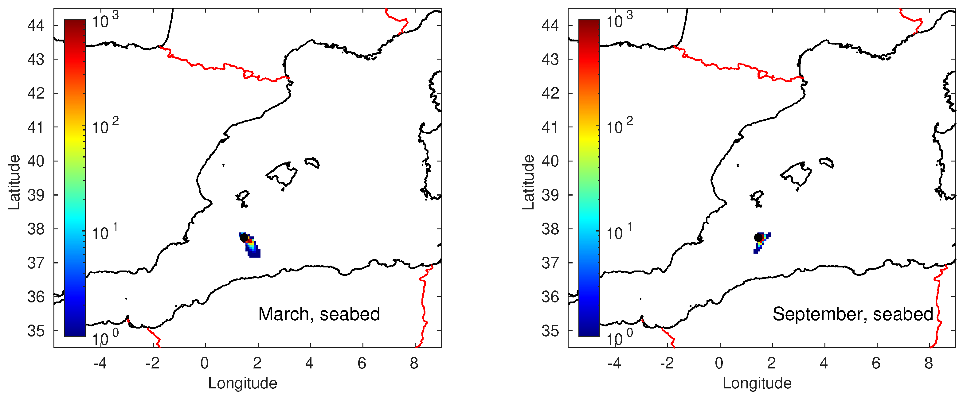
Resulting Pu distributions in bed sediments if the release occurs close to the seabed are presented in Figure 9, again using the accidents of March and September as examples. Only the sediments of the area around the accident location are affected by the release since Pu quickly attaches to solid particles and, consequently, its mobility is very low in the marine environment, as mentioned before. Peak concentrations are one order of magnitude higher than in the previous case, since all radionuclides are located in a small area.
4. Conclusions
A Lagrangian model, working in spherical coordinates, was developed to simulate the transport of radionuclides in the western Mediterranean Sea. The model includes the processes of advection by currents, three-dimensional mixing induced by turbulence, radioactive decay, and exchanges of radionuclides between water and the seabed sediments. These exchanges are described through a dynamic model based on kinetic transfer coefficients. Mixing, decay, and water/sediment interactions are solved applying a stochastic method. The water circulation was obtained from the HYCOM global ocean model. The model can be used to simulate instantaneous or continuous radionuclide releases over any temporal scale, and it provides maps of radionuclide concentrations in water and sediments as well as radionuclide age distributions, which may be used to infer oceanographic information.
Several hypothetical accidents were simulated. If a release occurs from a coastal nuclear facility, in particular the Vandellós II nuclear power plant in northeast Spain, it was found that Pu stays very close to the release area due to the low mobility of this radionuclide in the marine environment. In the case of Cs, radionuclides can travel to long distances from the release point, reaching the Balearic Islands, African coasts, and a significant part of the Spanish coastline. The time of the year when the accident occurs affects the dispersion patterns, as detailed above. Sediments are contaminated over a narrow band along the Spanish coastline, and radionuclides also reach the shallower waters around the Balearic Islands.
Several examples of Pu releases occurring far from the coastline were also considered. If the release takes place at the sea surface, resulting Pu concentrations in water present a clear seasonality. Coastal sediments of the regions reached by the Pu patch are contaminated. If the Pu release occurs deeper in the water column (mid-depth and close to the seabed), radionuclides do not reach the water surface layer. Sediments of the isobath at which the release occurred are contaminated with Pu in the case of the mid-depth release. Only the area close to the accident is contaminated with Pu if the release occurs at the seabed. Seasonality effects in results are lost in both cases.
It is relevant to have this type of model ready to operate in areas which could be potentially exposed to a nuclear accident, and especially if such areas have a concentrated population, high touristic potential, and/or great ecological value, as is the case, for instance, for the eastern coast of Spain and the Balearic Islands.
Author Contributions
R.P. and C.C.: conceptualization, software and analysis of results; R.P.: main writing; C.C.: writing and review. All authors have read and agreed to the published version of the manuscript.
Funding
This research received no external funding.
Institutional Review Board Statement
Not applicable.
Informed Consent Statement
Not applicable.
Data Availability Statement
Contact the authors.
Conflicts of Interest
The authors declare no conflict of interest.
References
- IAEA. Modelling of Marine Dispersion and Transfer of Radionuclides Accidentally Released from Land Based Facilities; IAEA–TECDOC–1876; IAEA: Vienna, Austria, 2019. [Google Scholar]
- Periáñez, R. Models for predicting the transport of radionuclides in the Red Sea. J. Environ. Radioact. 2020, 223–224, 106396. [Google Scholar] [CrossRef] [PubMed]
- Periáñez, R.; Min, B.-I.; Suh, K.-S. The transport, effective half-lives and age distributions of radioactive releases in the northern Indian Ocean. Mar. Pollut. Bull. 2021, 169, 112587. [Google Scholar] [CrossRef] [PubMed]
- Periáñez, R. APERTRACK: A particle-tracking model to simulate radionuclide transport in the Arabian/Persian Gulf. Progr. Nucl. Energ. 2021, 142, 103998. [Google Scholar] [CrossRef]
- Periáñez, R. A Lagrangian tool for simulating the transport of chemical pollutants in the Arabian/Persian Gulf. Modelling 2021, 2, 675–685. [Google Scholar] [CrossRef]
- Tsabaris, C.; Eleftheriou, G.; Tsiaras, K.; Triantafyllou, G. Distribution of dissolved 137Cs, 131I and 238Pu at eastern Mediterranean Sea in case of hypothetical accident at the Akkuyu nuclear power plant. J. Environ. Radioact. 2022, 251–252, 106964. [Google Scholar] [CrossRef]
- Bleck, R. An oceanic general circulation model framed in hybrid isopycnic–Cartesian coordinates. Ocean Model. 2001, 4, 55–88. [Google Scholar] [CrossRef]
- Xu, X.; Chassignet, E.P.; Price, J.F.; Özgökmen, T.M.; Peters, H. A regional modeling study of the entraining Mediterranean outflow. J. Geophys. Res. 2007, 112, C12005. [Google Scholar] [CrossRef] [Green Version]
- Kara, A.B.; Wallcraft, A.J.; Martin, P.J.; Pauley, R.L. Optimizing surface winds using QuikSCAT measurements in the Mediterranean Sea during 2000–2006. J. Mar. Syst. 2009, 78, S119–S131. [Google Scholar] [CrossRef]
- Pugh, D.T. Tides, Surges and Mean Sea Level; Wiley: Chichester, UK, 1987; p. 472. [Google Scholar]
- Periáñez, R.; Elliott, A.J. A particle tracking method for simulating the dispersion of non conservative radionuclides in coastal waters. J. Environ. Radioact. 2002, 58, 13–33. [Google Scholar] [CrossRef]
- Cushman-Roisin, B.; Beckers, J.M. Introduction to Geophysical Fluid Dynamics; Elsevier: Amsterdam, The Netherlands, 2011. [Google Scholar]
- Periáñez, R.; Bezhenar, R.; Brovchenko, I.; Jung, K.T.; Kamidara, Y.; Kim, K.O.; Kobayashi, T.; Liptak, L.; Maderich, V.; Min, B.I.; et al. Fukushima 137Cs releases dispersion modelling over the Pacific Ocean. Comparisons of models with water, sediment and biota data. J. Environ. Radioact. 2019, 198, 50–63. [Google Scholar] [CrossRef]
- D’Ortenzio, F.; Iudicone, D.; de Boyer Montegut, C.; Testor, P.; Antoine, D.; Marullo, S.; Santoleri, R.; Madec, G. Seasonal variability of the mixed layer depth in the Mediterranean Sea as derived from in situ profiles. Geophys. Res. Lett. 2005, 32, L12605. [Google Scholar] [CrossRef] [Green Version]
- Periáñez, R.; Brovchenko, I.; Jung, K.T.; Kim, K.O.; Maderich, V. The marine kd and water/sediment interaction problem. J. Environ. Radioact. 2018, 192, 635–647. [Google Scholar] [CrossRef]
- Periáñez, R. Modelling the environmental behavior of pollutants in Algeciras Bay (south Spain). Mar. Pollut. Bull. 2012, 64, 221–232. [Google Scholar] [CrossRef]
- Periáñez, R.; Suh, K.S.; Min, B.I.; Villa, M. The behaviour of 236U in the North Atlantic Ocean assessed from numerical modelling: A new evaluation of the input function into the Arctic. Sci. Total Environ. 2018, 626, 255–263. [Google Scholar] [CrossRef]
- Periáñez, R.; Hierro, A.; Bolivar, J.P.; Vaca, F. The geochemical behavior of natural radionuclides in coastal waters: A modelling study for the Huelva estuary. J. Marine Syst. 2013, 126, 82–93. [Google Scholar] [CrossRef]
- Periáñez, R. A modelling study on 137Cs and 239,240Pu behaviour in the Alborán Sea, western Mediterranean. J. Environ. Radioact. 2008, 99, 694–715. [Google Scholar] [CrossRef]
- Periáñez, R.; Bezhenar, R.; Brovchenko, I.; Duffa, C.; Iosjpe, M.; Jung, K.T.; Kobayashi, T.; Liptak, L.; Little, A.; Maderich, V.; et al. Marine radionuclide transport modelling: Recent developments, problems and challenges. Environ. Modell. Softw. 2019, 122, 104523. [Google Scholar] [CrossRef]
- Periáñez, R.; Suh, K.S.; Min, B.I. Should we measure plutonium concentrations in marine sediments near Fukushima? J. Radioanal. Nucl. Chem. 2013, 298, 635–638. [Google Scholar] [CrossRef]
- IAEA. Sediment Distribution Coefficients and Concentration Factors for Biota in the Marine Environment; Technical Reports Series 422; IAEA: Vienna, Austria, 2004. [Google Scholar]
- Nyffeler, U.P.; Li, Y.H.; Santschi, P.H. A kinetic approach to describe trace element distribution between particles and solution in natural aquatic systems. Geochim. Cosmochim. Acta 1984, 48, 1513–1522. [Google Scholar] [CrossRef]
- Deleersnijder, E.; Capin, J.M.; Delhez, E.J.M. The concept of age in marine modelling 1: Theory and preliminary model results. J. Marine Syst. 2001, 28, 229–267. [Google Scholar] [CrossRef]
- Periáñez, R. Modelling the Transport of Radionuclides in the Marine Environment: An Introduction; Springer: Berlin/Heidelberg, Germany, 2005. [Google Scholar]
- Periáñez, R.; Brovchenko, I.; Duffa, C.; Jung, K.T.; Kobayashi, T.; Lamego, F.; Maderich, V.; Min, B.I.; Nies, H.; Osvath, I.; et al. A new comparison of marine dispersion model performances for Fukushima Dai–ichi releases in the frame of IAEA MODARIA program. J. Environ. Radioact. 2015, 150, 247–269. [Google Scholar] [CrossRef] [PubMed]
- Periáñez, R.; Suh, K.S.; Min, B.I. The behaviour of 137Cs in the North Atlantic Ocean assessed from numerical modelling: Releases from nuclear fuel reprocessing factories, redissolution from contaminated sediments and leakage from dumped nuclear wastes. Mar. Pollut. Bull. 2016, 13, 343–361. [Google Scholar] [CrossRef] [PubMed]
- Periáñez, R.; Bezhenar, R.; Iosjpe, M.; Maderich, V.; Nies, H.; Osvath, I.; Outola, I.; de With, G. A comparison of marine radionuclide dispersion models for the Baltic Sea in the frame of IAEA MODARIA program. J. Environ. Radioact. 2015, 139, 66–77. [Google Scholar] [CrossRef] [PubMed]
- Kobayashi, T.; Nagai, H.; Chino, M.; Kawamura, H. Source term estimation of atmospheric release due to the Fukushima Dai–ichi Nuclear Power Plant accident by atmospheric and oceanic dispersion simulations. J. Nucl. Sci. Technol. 2013, 50, 255–264. [Google Scholar] [CrossRef] [Green Version]
- Christoudias, T.; Lelieveld, J. Modelling the global atmospheric transport and deposition of radionuclides from the Fukushima Dai–ichi nuclear accident. Atmos. Chem. Phys. 2013, 13, 1425–1438. [Google Scholar] [CrossRef] [Green Version]
- Bezhenar, R.; Heling, R.; Ievdin, I.; Iosjpe, M.; Maderich, V.; Willemsen, S.; de With, G.; Dvorzhak, A. Integration of marine food chain model POSEIDON in JRODOS and testing versus Fukushima data. Radioprotection 2016, 51, S137–S139. [Google Scholar] [CrossRef] [Green Version]
- Papucci, C.; Delfanti, R. 137-Caesium distribution in the eastern Mediterranean Sea: Recent changes and future trends. Sci. Total Environ. 1999, 237–238, 67–75. [Google Scholar] [CrossRef]
- Evangeliou, N.; Florou, H.; Kritidis, P. A Survey of 137Cs in Sediments of the Eastern Mediterranean Marine Environment from the Pre-Chernobyl Age to the Present. Environ. Sci. Technol. Lett. 2014, 1, 102–107. [Google Scholar] [CrossRef]
- Zheng, J.; Aono, T.; Uchida, S.; Zhang, J.; Honda, M.C. Distribution of Pu isotopes in marine sediments in the Pacific 30 km off Fukushima after the Fukushima Daiichi nuclear power plant accident. Geochem. J. 2012, 46, 361–369. [Google Scholar] [CrossRef] [Green Version]
- Papucci, C. Time evolution and levels of man–made radioactivity in the Mediterranean sea. In Radionuclides in the Oceans; Gurgurniat, P., Germain, P., Mrtivier, H., Eds.; Les Editions de Physique: Les Ulis, France, 1996; pp. 177–197. [Google Scholar]
- Smith, J.N.; Ellis, K.M.; Aarkrog, A.; Dahlgaard, H.; Holm, E. Sediment mixing and burial of the plutonium–239/240 pulse from the 1968 Thule Greenland nuclear weapon accident. J. Environ. Radioact. 1994, 25, 135–159. [Google Scholar] [CrossRef]
- Sivintsev, Y. Study of Nuclide Composition and Characteristics of Fuel in Dumped Submarine Reactors and Atomic Icebreaker `Lenin’, Part I—Atomic Icebreaker; IAEA–IASAP–1; IAEA: Vienna, Austria, 1994. [Google Scholar]
- IAEA. Predicted Radionuclide Release from Marine Reactors Dumped in the Western Kara Sea; Report of the Source Term Working Group of the International Arctic Seas Assessment Project (IASAP), IAEA–TECDOC–938; IAEA: Vienna, Austria, 1997. [Google Scholar]
- Lee, S.H.; La Rosa, J.J.; Levy-Palomo, I.; Oregioni, B.; Pham, M.K.; Povinec, P.P.; Wyse, E. Recent inputs and budgets of 90Sr, 137Cs, 239,240Pu and 241Am in the northwest Mediterranean Sea. Deep Sea Res. Pt. II 2003, 50, 2817–2834. [Google Scholar] [CrossRef]
- Lansard, B.; Charmasson, S.; Gascó, C.; Antón, M.P.; Grenz, C.; Arnaud, M. Spatial and temporal variations of plutonium isotopes (238Pu and 239,240Pu) in sediments off the Rhone River mouth (NW Mediterranean). Sci. Total Environ. 2007, 376, 215–227. [Google Scholar] [CrossRef]
Figure 1.
Example of surface circulation in the western Mediterranean (31 January), as downloaded from the HYCOM ocean model. Only one of each of the 16 current vectors are drawn for more clarity. The dot indicates the location of the Vandellós II nuclear power plant in Spain.
Figure 1.
Example of surface circulation in the western Mediterranean (31 January), as downloaded from the HYCOM ocean model. Only one of each of the 16 current vectors are drawn for more clarity. The dot indicates the location of the Vandellós II nuclear power plant in Spain.

Figure 2.
Calculated Cs concentrations in surface water (Bq/m) three months after hypothetical accidents in the Vandellós II nuclear power plant starting on 21 March, 21 June, 21 September, and 21 December.
Figure 2.
Calculated Cs concentrations in surface water (Bq/m) three months after hypothetical accidents in the Vandellós II nuclear power plant starting on 21 March, 21 June, 21 September, and 21 December.

Figure 3.
Calculated Cs age distributions in surface water (days) after hypothetical accidents in the Vandellós II nuclear power plant starting on 21 March, 21 June, 21 September, and 21 December.
Figure 3.
Calculated Cs age distributions in surface water (days) after hypothetical accidents in the Vandellós II nuclear power plant starting on 21 March, 21 June, 21 September, and 21 December.

Figure 4.
Calculated Cs concentrations in bed sediments (Bq/m) three months after hypothetical accidents in the Vandellós II nuclear power plant starting on 21 March, 21 June, 21 September, and 21 December.
Figure 4.
Calculated Cs concentrations in bed sediments (Bq/m) three months after hypothetical accidents in the Vandellós II nuclear power plant starting on 21 March, 21 June, 21 September, and 21 December.

Figure 5.
Calculated Cs age distributions in bed sediments (days) after hypothetical accidents in the Vandellós II nuclear power plant starting on 21 March, 21 June, 21 September, and 21 December.
Figure 5.
Calculated Cs age distributions in bed sediments (days) after hypothetical accidents in the Vandellós II nuclear power plant starting on 21 March, 21 June, 21 September, and 21 December.

Figure 6.
Calculated Pu concentrations in surface water (Bq/m) after a hypothetical instantaneous release occurring on the sea surface on 21 March, 21 June, 21 September, and 21 December. The dot indicates the accident location.
Figure 6.
Calculated Pu concentrations in surface water (Bq/m) after a hypothetical instantaneous release occurring on the sea surface on 21 March, 21 June, 21 September, and 21 December. The dot indicates the accident location.

Figure 7.
Calculated Pu concentrations in bed sediments (Bq/m) after a hypothetical instantaneous release occurring on the sea surface on 21 March, 21 June, 21 September, and 21 December. The dot indicates the accident location.
Figure 7.
Calculated Pu concentrations in bed sediments (Bq/m) after a hypothetical instantaneous release occurring on the sea surface on 21 March, 21 June, 21 September, and 21 December. The dot indicates the accident location.

Figure 8.
Calculated Pu concentrations in bed sediments (Bq/m) after a hypothetical instantaneous release occurring at 1500 m depth on 21 March and 21 September. The dot indicates the accident location.
Figure 8.
Calculated Pu concentrations in bed sediments (Bq/m) after a hypothetical instantaneous release occurring at 1500 m depth on 21 March and 21 September. The dot indicates the accident location.

Figure 9.
Calculated Pu concentrations in bed sediments (Bq/m) after a hypothetical instantaneous release occurring at 2990 m depth on 21 March and 21 September. The dot indicates the accident location.
Figure 9.
Calculated Pu concentrations in bed sediments (Bq/m) after a hypothetical instantaneous release occurring at 2990 m depth on 21 March and 21 September. The dot indicates the accident location.

Disclaimer/Publisher’s Note: The statements, opinions and data contained in all publications are solely those of the individual author(s) and contributor(s) and not of MDPI and/or the editor(s). MDPI and/or the editor(s) disclaim responsibility for any injury to people or property resulting from any ideas, methods, instructions or products referred to in the content. |
© 2023 by the authors. Licensee MDPI, Basel, Switzerland. This article is an open access article distributed under the terms and conditions of the Creative Commons Attribution (CC BY) license (https://creativecommons.org/licenses/by/4.0/).
Share and Cite
MDPI and ACS Style
Periáñez, R.; Cortés, C. A Numerical Model to Simulate the Transport of Radionuclides in the Western Mediterranean after a Nuclear Accident. J. Mar. Sci. Eng. 2023, 11, 169. https://doi.org/10.3390/jmse11010169
AMA Style
Periáñez R, Cortés C. A Numerical Model to Simulate the Transport of Radionuclides in the Western Mediterranean after a Nuclear Accident. Journal of Marine Science and Engineering. 2023; 11(1):169. https://doi.org/10.3390/jmse11010169
Chicago/Turabian StylePeriáñez, Raúl, and Carmen Cortés. 2023. "A Numerical Model to Simulate the Transport of Radionuclides in the Western Mediterranean after a Nuclear Accident" Journal of Marine Science and Engineering 11, no. 1: 169. https://doi.org/10.3390/jmse11010169
Note that from the first issue of 2016, this journal uses article numbers instead of page numbers. See further details here.