Numerical Study of Influences of Onshore Wind on Hydrodynamic Processes of Solitary Wave over Fringing Reef

Abstract

Many post-disaster surveys have reported on the natural function and effectiveness of fringing reef in preventing the shoreline from the inundation caused by severe weather events. Prior studies mainly focus on the wave propagating, transforming, and breaking on the fringing reefs by assuming that ocean waves propagate in an ideal environment where the wind is absent. However, in the real severe ocean environment, huge surges and waves always occur simultaneously with the strong winds. The wave profile can be easily reshaped by the strong winds, which can also significantly affect the way that ocean waves propagate on the fringing reefs. Therefore, it is necessary to study the hydrodynamics of fringing reefs under the combined action of wind and waves. To study the influences of the onshore wind on the hydrodynamics of solitary wave on the fringing reef, the finite volume method is applied to solve the governing equations of two-phase incompressible flow and a high-resolution numerical wind-wave tank is established in this study. Effects of several main factors are analyzed in detail. The research results show that the onshore wind can significantly increase the maximum wave runup height (maximum by 38.49%) and decrease the wave reflection coefficient of solitary wave (maximum by 8.66%). It is hoped that the research results of this study can enhance the understandings on the hydrodynamics of ocean waves on the fringing reefs during severe weather events.

1. Introduction

Fringing reefs are distributed widely along the coastline in subtropical or tropical regions, which consist of a steep offshore forereef slope, a shallow reef flat, and a steep backreef beach [1,2]. Most of the incident ocean wave energy can be dissipated through the wave breaking processes near the reef edge or reef crest. As the breaking surge bore propagates on the reef flat, the rest of ocean wave energy can be further lost due to the frictional force at the rough bottom [3,4]. The natural buffer capability of fringing reefs in preventing the coastlines from the inundation induced by the harsh weather events has been reported in many post-disaster surveys [5,6,7]. However, influences of the onshore winds are often ignored in the previous research when the wave hydrodynamics of fringing reefs are considered, although the huge waves are always accompanied by the strong coastal winds during extreme events. Hence, it is significantly necessary to investigate the influences of wind on the hydrodynamic processes of solitary wave on the fringing reefs, which is also a necessary supplement to the previous studies.

The complex interactions between the different kinds of incident waves, i.e., regular wave [8,9,10,11] and random waves [12,13,14], and the fringing reefs have been extensively studied though field-surveys [15], theoretical analysis [16], laboratory experiments [17], and numerical simulations [18,19]. Since the low-laying reef coasts are vulnerable to the inundations during the extreme weather events, many efforts have been devoted to investigating the wave setup over the reef flat [20] and wave runup processes at the backreef slope [21]. The previous research findings revealed that the infragravity waves can become dominant in the shoreline wave runup processes at the backreef slope after the majority of the wave energy of sea and swell waves is dissipated by the wave breaking processes and the frictional forces at the rough bottom of reef flat [22]. The maximum value of wave runup height of the infragavity waves can be further enhanced by the reef flat resonance [23]. Effects of reef morphology [24], anthropic excavation pit [25], seawall [26], and bottom roughness on this process were also systematically investigated in recent years. These studies have undoubtedly promoted the understandings on the hydrodynamic processes of ocean waves on the fringing reefs.

However, very limited studies were performed on the hydrodynamic processes of solitary wave on the fringing reefs [27]. For instance, Roeber and his colleagues [28,29] studied the hydrodynamics of two-dimensional (2D) reef configurations under solitary wave in a wave flume. Based on the experiment data collected in Roeber et al. [28], Kazolea et al. [30] numerically evaluated the performances of several different types of flow solvers in modelling the transforming and breaking of solitary wave on different fringing reefs. Quiroga and Cheung [31] and Yao et al. [7] both systematically investigated the effects of bed-form roughness of the reef surfaces on the hydrodynamics of solitary wave on the fringing reefs through both laboratory experiments and numerical simulations. Their results revealed that the bed-form roughness can significantly increase the bottom friction and greatly enhance the wave energy dissipation rate during the shoaling process of solitary wave. Moreover, Liu et al. [32] numerically investigated the momentum flux properties of solitary wave on the fringing reefs. Qu et al. [33] investigated the influences of permeability of the reef flat on the hydrodynamic processes of solitary wave on the fringing reef. Their results indicate that if the classical quadratic friction law is applied to approximate the friction forces at the rough bottom of fringing reef, the wave energy dissipation rate can be greatly underestimated.

During the coastal harsh weather events, the generation, propagation, and transformation of the huge surges and waves are always accompanied by the strong onshore winds. The earliest studies of wind–wave interactions can date back to the 1920s, when Jeffrey [34] studied the generation mechanism of ocean surface waves by the action of wind. Subsequently, several scholars carried out similar studies successively, and focused on the analysis of the air separation processes over wave surfaces [35,36]. For a long time after that, study on the wind–wave interactions did not attract enough attention from the research community. In recent years, many laboratory experiments were carried out to understand the influences of winds on the nearshore wave shoaling and breaking [37,38] and their influences on the coastal sediment transportation [39]. It is reported that even light-wind can finally influence the wave breaking processes [40]. Moreover, influences of the onshore winds on the propagations of freak wave groups have been systematically investigated through both experiment works [41,42] and numerical simulations [43,44,45]. It is found that the actual focusing location can be shifted downward by the onshore wind and the peak wave height can be increased. The hydrodynamic loads of coastal structures under the combined action of wind and waves were also studied in recent years. For instance, the complicated interactions between the regular waves and onshore wind at a seawall was numerically studied by Hieu et al. [46]. Their research findings indicated that the presence of wind can significantly increase the wave-overtopping rate at the vertical seawall. By applying a two-phase numerical wind-wave tank, Qu et al. [47] and Wen et al. [48] studied the influences of onshore wind on the hydrodynamics of coastal bridge decks under the actions of solitary wave or regular waves, respectively.

So far, there are few studies that have been performed to investigate the influences of wind on the hydrodynamics of fringing reef under the ocean waves. In the past, several tsunami events have caused massive socio-economic and human losses in the coastal regions where the tsunami-induced floodings can easily reached. During harsh weather conditions, the tsunami waves can become more devastating to the coast. Although the rationality of using the solitary wave as a tsunami wave model is questioned in recent years, the solitary wave is widely applied since it shares some main facets of tsunami waves. To make up for the shortcomings of previous studies, influences of the onshore winds on the hydrodynamics of solitary wave on the fringing reef have been numerically analyzed based on a two-phase numerical wind-wave tank. Influences of several main factors, i.e., onshore wind speed, water depth, wave height, and forereef and backreef slopes, are discussed in detail.

The remainder of the paper is organized as follows. The descriptions on the numerical wind-wave tank are given in Section 2. Model validation is performed in Section 3. Section 4 presents the discussions on the research results. Section 5 summarizes the research findings.

2. Descriptions on Numerical Model

The complex hydrodynamics of solitary wave on the fringing reef can be fully described by the unsteady two-phase incompressible flow, whose governing equations can be formulated as

$$\frac{\partial u_i}{\partial x_i}=0$$

(1)

$$\frac{\partial \rho u_i}{\partial t}+\rho u_j\frac{\partial u_i}{\partial x_j}=-\frac{\partial p}{\partial x_i}+\frac{\partial }{x_j}\left[{\mu }_{eff}\left(\frac{\partial u_i}{\partial x_j}+\frac{\partial u_j}{\partial x_i}\right)\right]+\rho g_i$$

(2)

where $u_i$ is the velocity, $p$ is the pressure, $t$ is the time,$\rho$ is the flow density, ${\mu }_{eff}={\mu }_l+{\mu }_t$ is the effective viscosity, ${\mu }_l$ is the laminar viscosity, ${\mu }_t$ is the turbulence viscosity, and $g_i$ is the gravity acceleration. The finite volume method (FVM) has been applied to numerically integrate the governing Equations (1) and (2) [49,50]. To avoid the numerical instability issue, the momentum interpolation method has been applied to interpolate the velocities at the cell faces from the control cell centers [51]. The pressure and velocity are coupled by applying the classical Pressure Implicit Split Operator (PISO) method [52].

The turbulence closure is met by applying the classic $k$ − $\omega$ turbulence model [53], whose governing equations for the kinetic energy ($k$) and the specific turbulent dissipation ($\omega$) can be formulated as

$$\frac{\partial \rho k}{\partial t}+\rho u_j\frac{\partial k}{\partial x_j}=\frac{\partial }{\partial x_j}\left[\left({\mu }_l+\frac{{\mu }_t}{{\sigma }_k}\right)\frac{\partial k}{\partial x_j}\right]+2{\mu }_t{\left|S\right|}^2-\rho k\omega$$

(3)

$$\frac{\partial \rho \omega }{\partial t}+\rho u_j\frac{\partial \omega }{\partial x_j}=\frac{\partial }{\partial x_j}\left[\left({\mu }_l+\frac{{\mu }_t}{{\sigma }_{\omega }}\right)\frac{\partial \omega }{\partial x_j}\right]+2c_{\mu }{c}_{\omega 1}\rho {\left|S\right|}^2-c_{\omega 2}\rho {\omega }^2$$

(4)

The turbulent viscosity can be calculated by ${\mu }_t=\rho k/\omega$. As suggested in [48], $c_{\mu }=0.09$, $c_{\omega 1}=5/9$, $c_{\omega 2}=5/6$, and ${\sigma }_{\omega }={\sigma }_k=2$. The term ${\left|S\right|}^2$ is constituted of the mean rate of the strain tensor

$$S=\frac{1}{2}\left(\frac{\partial u_j}{\partial x_i}+\frac{\partial u_i}{\partial x_j}\right)$$

(5)

In the following computations, the initial turbulent kinetic energy is set as 0 ${\mathrm{m}}^2/{\mathrm{s}}^2$, and the initial specific dissipation rate is set as 1.0 ${\mathrm{s}}^{-1}$.

To accurately compute the interface between the air and water, the volume of fluid method (VOF) is used in this study. The transportation of VOF can be described by

$$\frac{\partial \gamma }{\partial t}+\frac{\partial \gamma u_i}{\partial x_i}=0$$

(6)

where $\gamma$ represents the volume fluid of water in a cell and is defined by whether the control volume is filled by water or air, as

$$\left\{\begin{array}{cc}\hspace{1em} \gamma =0,& air\hfill \\ 0<\gamma <1,& interface\hfill \\ \hspace{1em} \gamma =1,& water\hfill \end{array}\right.$$

(7)

The flow density and the flow laminar viscosity can be defined as functions of $\gamma$, as

$$\rho ={\rho }_{air}+\gamma ·\left({\rho }_{water}-{\rho }_{air}\right)$$

(8)

$${\mu }_l={\mu }_{air}+\gamma ·\left({\mu }_{water}-{\mu }_{air}\right)$$

(9)

In this study, one of the high-resolution VOF methods named STACS (Switching Technique for Advection and Capturing of Surfaces) was used [54].

To quantitively evaluate the wave hydrodynamics of solitary wave on the fringing reef, the wave reflection coefficient is defined as

$$C_R=\frac{H_R}{H_I}$$

(10)

where $H_I$ is the incident wave height and $H_R$ is the reflected wave height. In addition, the units of physical quantities represented by all symbols in this paper are SI units.

3. Model Verification

In order to calibrate the reliability of present numerical wave model, hydrodynamics of a solitary wave on the fringing reef model are numerically simulated. The computed water elevations and wave runup process are verified by the experiment data [27]. Figure 1 depicts the experimental layout of the fringing reef model. In the experiment, six capacitance-wire wave gauges were placed laterally along the flume to record the solitary wave propagation, shoaling and breaking process over the fringing reefs. To measure the wave run-up height, a 2 m capacitance-wire wave gauge was laid on the back-reef slope. The fringing reef model is composed of a forereef slope (1:3), a 4.93 m wide horizontal reef flat with a reef height of 0.383 m, and a backreef slope (1:11.9). The toe of the forereef slope is installed at 14.25 m away from the wave paddle. In the simulation, the wave height ($H$) is 0.05 m. The water depth ($h$) is 0.413 m. Moreover, 40 mesh layers have been applied to discretize the region of wave height. The computed temporal evolutions of water surface elevation recorded at x = 8.25, 14.25, 14.825, 15.4, 17.387, 20.33 m are compared with measured data, as shown in Figure 2. The computed water surface elevations are in good agreement with the measured data. The skill number [55] is applied to assess the degree of agreement between numerical results and experimental data. The skill numbers for the water surface elevations at different wave gauges are all greater than 0.85, indicating that the computed water surface elevations are in good agreement with the experiment data. Figure 3 compares the time series of computed and measured wave runup processes at the backreef slope. The computed wave runup height can well match the measurement. The difference in the maximum value of wave runup between the prediction and the measurement is less than 6%. Overall, the present numerical wave model can well resolve the full hydrodynamics of a solitary wave on the fringing reef.

4. Discussion on Results

Hydrodynamic processes of the solitary wave in windy condition on the fringing reef have been systematically analyzed. Influences of several main factors, i.e., the onshore wind speed, water depth, wave height, and forereef and backreef slopes are carefully discussed. Similar to [27], the computational layout is plotted in Figure 4. As depicted in Figure 4, the length of reef flat is 4.93 m. The reef height is 0.383 m. $\alpha$ and $\beta$ represent the forereef and backreef slope angle, respectively. For the basic run, the forereef slope ($\tan \alpha$) is 1:3, and the backreef slope ($\tan \beta$) is 1:10. The toe of the forereef slope is located 14.25 m away from the inlet. In this study, time series of water elevation and horizontal wind velocity in the logarithmic profile are imposed at the inlet, as depicted in Figure 1. The wind speed ($U_w$) imposed at the inlet represents the averaged wind speed, which is normalized by the shallow water celerity ($C$) in this study as $U_w^{*}=U_w/C$ and $C=\sqrt{gh}$.

In this study, the logarithmic wind profile at the inlet is defined as

$$u_w\left(z\right)=\frac{u_{*}}{\kappa }ln\left(\frac{z}{z_0}\right)$$

(11)

The friction velocity is defined as $u_{*}=\kappa U_w/ln\left(\delta /z_0\right)$. $\delta$ is the distance between the water surface and the top of the computational domain at the inlet. The von Karman constant $\kappa$ = 0.4. $z_0$ is the surface roughness. For the smooth open water surface, $z_0$ is set as 0.0002 m in this study.

In addition, to adapt to the temporal evolution of the water elevation at the inlet, the lowest boundary of the wind at the inlet needs to evolve closely with the temporal evolution of water elevation of solitary wave [47]. In our previous studies [47,48], the computational capability of the present numerical model in predicting the complex interactions between the waves and the wind has been well verified. For interested readers, please refer to [47,48].

4.1. Hydrodynamic Analyses

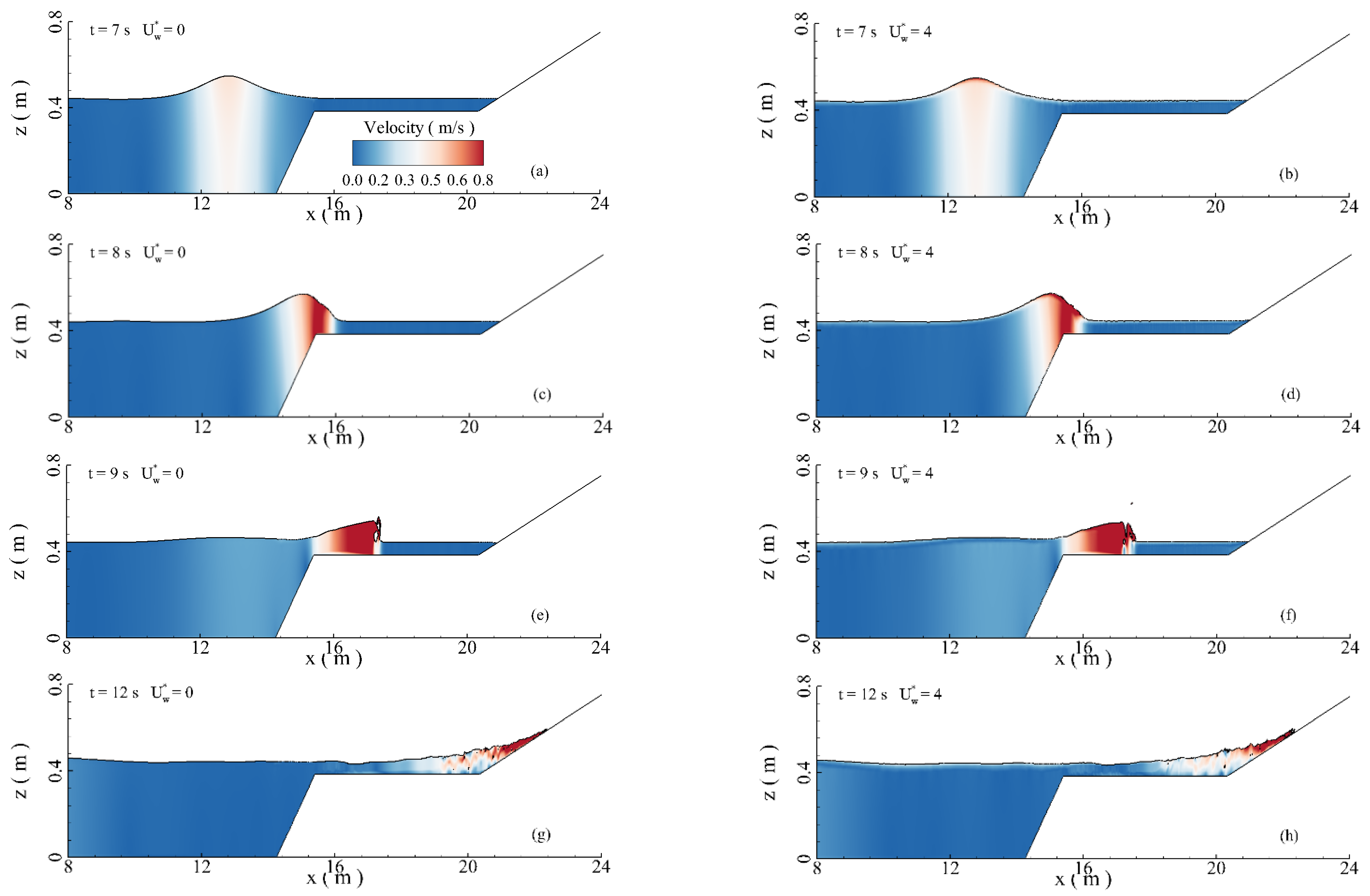
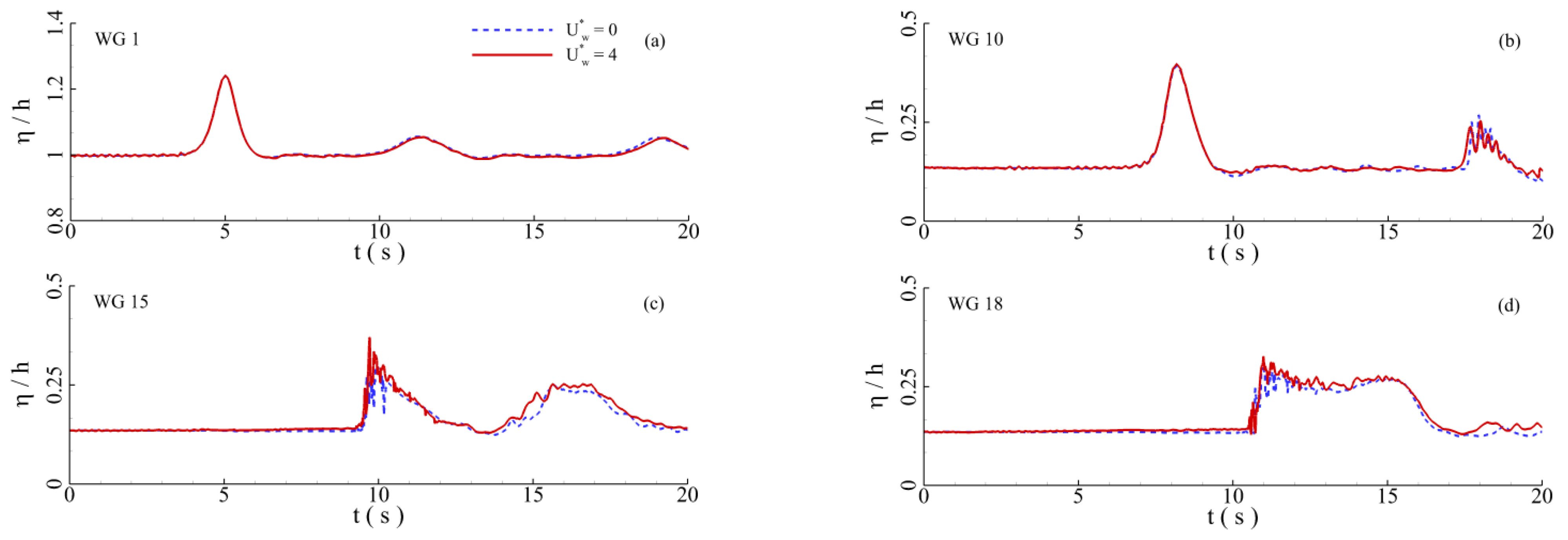
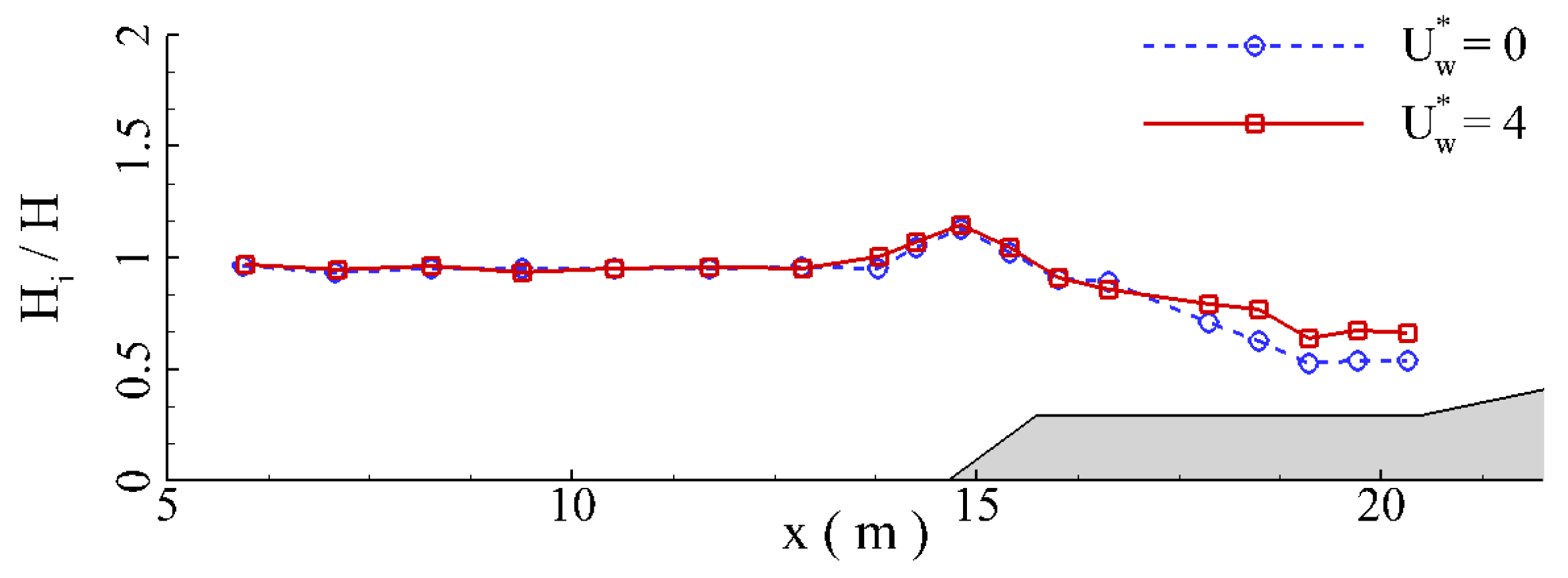
In this section, influences of the onshore wind on the complex hydrodynamic processes of solitary wave on the fringing reef are analyzed. The water depth ($h$) is 0.443 m. The wave height ($H$) is 0.11075 m. The relative wave height ($\epsilon =H/h$) is 0.25. The submergence water depth ($h_r$) is 0.06 m. The wind speed ($U_w$) is 4$C$, and $C$ = 2.085 m/s. Hence, the corresponding dimensionless wind speed $U_w^{*}$ = 4. Figure 5 depicts the plots of water velocity contour at different time moments. As the onshore wind blows over the water surface, the significant velocity differences between the water and air phases results in a strong wind shear stress at the water surface. Moreover, as the onshore wind blows over the crest of solitary wave, air separation can be formed, which can produce a strong pressure imbalance. Driven by the wind stress sand pressure forces, water layer in the high velocity can be observed near the surface of the water body (Figure 5a). Attributed to the blowing influences of onshore wind, the solitary wave shape gradually becomes asymmetrical. Meanwhile, noticeable water surface oscillations can be observed, especially in the leeward region. As the solitary wave propagates over the forereef slope, the wave steepness tends to increase. At this moment, the solitary wave will have a larger wave steepness under the action of onshore wind (Figure 5b). Under the continuous action of blowing wind, the speed of the water body of solitary wave will continue to increase, eventually leading to more complex and stronger wave breaking processes (Figure 5c). Under the driving forces of onshore wind, the breaking surge bore will produce a greater wave runup height (Figure 5d). Figure 6 plots the pressure contours of the water body different time moments. Obviously, compared to the solitary wave in the no-wind condition, due to the blowing action of onshore wind, low pressure region can be formed near wave crest or the front side of breaking surge bore, which can impose extra sucking force at the water surface due to the low pressure, resulting in the stronger wave breaking processes. Figure 7 shows the snapshots of the vector velocity field at the time instance of wave breaking. It is seen that the breaking intensity of a solitary wave can be strengthened by the strong onshore wind. Meanwhile, a big vortex structure can form at the front side of the breaking surge bore under the action of onshore wind. In addition, it is found that there exist vast differences in the velocity magnitude in the air and water phases when the onshore wind is present. The high velocity in the air phase and low speed in the water phase can generate a very high velocity gradient, which finally can cause high shear stress at the water surface. Figure 8 shows the contours of shear stress during the wave-breaking processes. It is seen clearly there exists higher shear stress at the air and water interface under the onshore wind. This finding is consistent with the results shown in Figure 7. Before the solitary wave approaching the reef edge, the presence of wind has few influences on the temporal evolutions of water elevations, as depicted in Figure 9a,b. Once the wave breaking occurs, the effects of onshore wind on the temporal evolutions of water elevation can be become more apparent. The presence of onshore wind can increase the peak values of water elevations, as shown in Figure 9c,d. Figure 10 shows the spatial distributions of local wave heights of the solitary wave in the windy and no-wind conditions. As depicted in Figure 10, it is found that the spatial distributions of solitary wave with and without the onshore wind nearly coincide with each other before the occurrence of wave breakings. Once the wave breaking occurs, the wind driving forces can significantly increase the local wave height. Figure 11 shows the temporal evolutions of wave runup height. It is seen that the wave runup of solitary wave in the windy condition occurs in advance a little bit. The maximum value of wave runup height of solitary wave in the windy condition can be 22.6% greater than that in no-wind condition. Overall, it is found that the presence of wind has significant influences on the hydrodynamic processes of solitary wave on the fringing reef.

4.2. Influences of Wind Speed

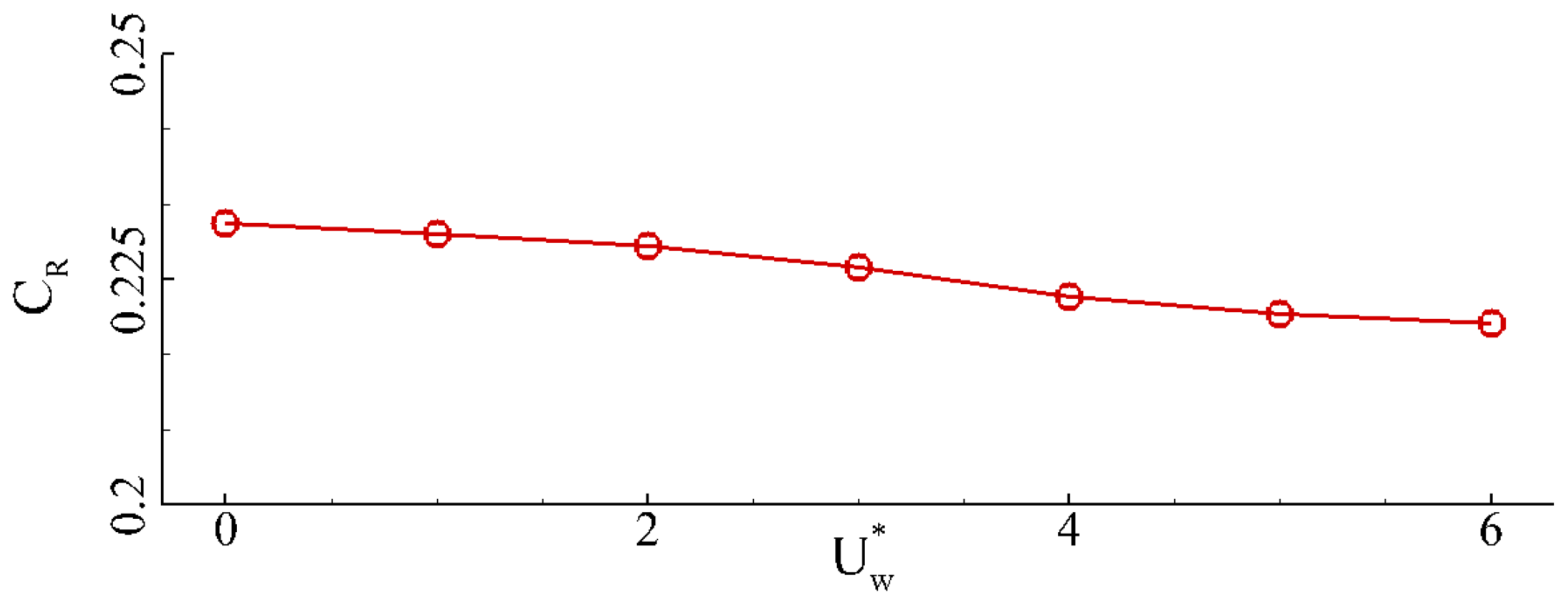
Influences of the wind speed on the hydrodynamics of solitary wave in the windy condition on the fringing reef are numerically investigated by selecting six different nondimensional wind speeds, i.e., $U_w^{*}$ = 0, 2, 3, 4, 5 and 6. Given the water depth ($h$) of 0.443 m, the selected six different nondimensional wind speed represent the wind speed $U_w$ = 0, 4.17, 6.255, 8.34, 10.425 and 12.51 m/s, respectively. The wave height ($H$) is 0.11075 m, and the relative wave height ($H/h$) is 0.25. The submergence depth ($h_r$) at the reef flat is 0.06 m. Figure 12 plots the water velocity contours at different time moments under different onshore wind speeds. As depicted in Figure 12, the flow velocity near the wave crest tends to increase with the onshore wind speed before the occur of wave breaking. At the same time, the flow velocity near the water surface also gradually increases with the onshore wind speed. Moreover, it is also observed that as the wind speed continues to increase, the time of occurrence of wave breaking continues to advance. Figure 13 depicts the spatial distributions of local wave heights of solitary wave under different onshore wind speeds. The local wave height of a solitary wave after the wave breakings gradually increases with the onshore wind speed. As seen in Figure 14, the wave reflection coefficient decreases gradually with the onshore wind speed. When the wind speed ($U_w^{*}$) increases from 0 to 6, the wave reflection coefficient decreases by 8.66%. It is attributed to reason that the propagation celerity of solitary wave gradually increases under the increasingly intensified blowing effects of onshore wind. Figure 15 shows the variations of the maximum value of wave runup height of solitary wave with the onshore wind speed. It is seen that the maximum value of wave runup height monotonically increases with the onshore wind speed in a linear mode. When the wind speed ($U_w^{*}$) increases from 0 to 6, the maximum value of wave runup height increases by 38.49%.

4.3. Influences of Wave Height and Water Depth

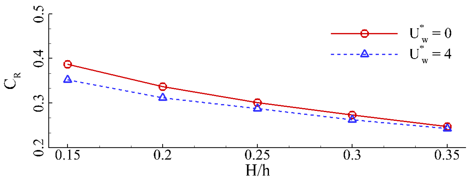
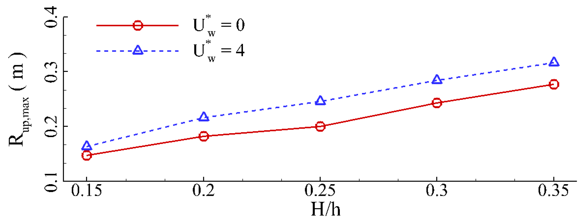
In this section, influences of the wave height and water depth on the hydrodynamics of solitary wave in the windy condition on the fringing reef are investigated. In the computation, the dimensionless wind speed is $U_w^{*}$ = 4. When the influences of wave height are discussed, the water depth ($h$) is 0.443 m. Five different relative wave heights are chosen, i.e., $H/h$ = 0.15, 0.2, 0.25, 0.3 and 0.35. Figure 16 plots the spatial distributions of the local wave heights under different relative wave heights. Driven by the blowing influences of onshore wind, the local wave height of solitary wave in the windy condition is generally greater than that in the no-wind condition after the wave breakings. Moreover, the variation trend of local wave height with the relative wave height after the wave breakings exhibit nonlinear behavior. For instance, when the relative wave height ($H/h$) is equal to 0.15 or 0.25, there exist apparent differences between the local wave heights of solitary wave in the windy and no-wind conditions after the wave breakings. However, when the relative wave height ($H/h$) is 0.2, the spatial distributions of local wave height of solitary wave in the windy and no-wind conditions almost coincide with each other. Figure 17 depicts the variation of the wave reflection coefficient of solitary wave with the relative wave height. When the relative wave height gradually increases, the wave reflection coefficient tends to decrease monotonically. Meanwhile, the differences in the wave reflection coefficients between the solitary wave in the windy and no-wind conditions tends to decrease as well. When the relative wave height ($H/h$) increases from 0.15 to 0.35, the wave reflection coefficient for the solitary wave in the windy and no-wind conditions decreases by 8.92% and 1.94%, respectively. The wave reflection coefficient of solitary wave in the no-wind condition is always greater than that of solitary wave in the windy condition, averagely 5.33% greater. Figure 18 depicts the variation of the maximum value of wave runup height of solitary wave on the fringing reef with the relative wave height. As depicted in Figure 17, the maximum value of wave height monotonically increases with the relative wave height for both solitary wave in the windy and no-wind conditions. When the relative wave height ($H/h$) increases from 0.15 to 0.35, the maximum value of wave runup height of solitary wave in the windy and no-wind conditions increases by 10.95% and 13.98%, respectively. The maximum value of wave runup height of solitary wave in the windy condition is always greater than that in the no-wind condition, on average, 16.67% greater.

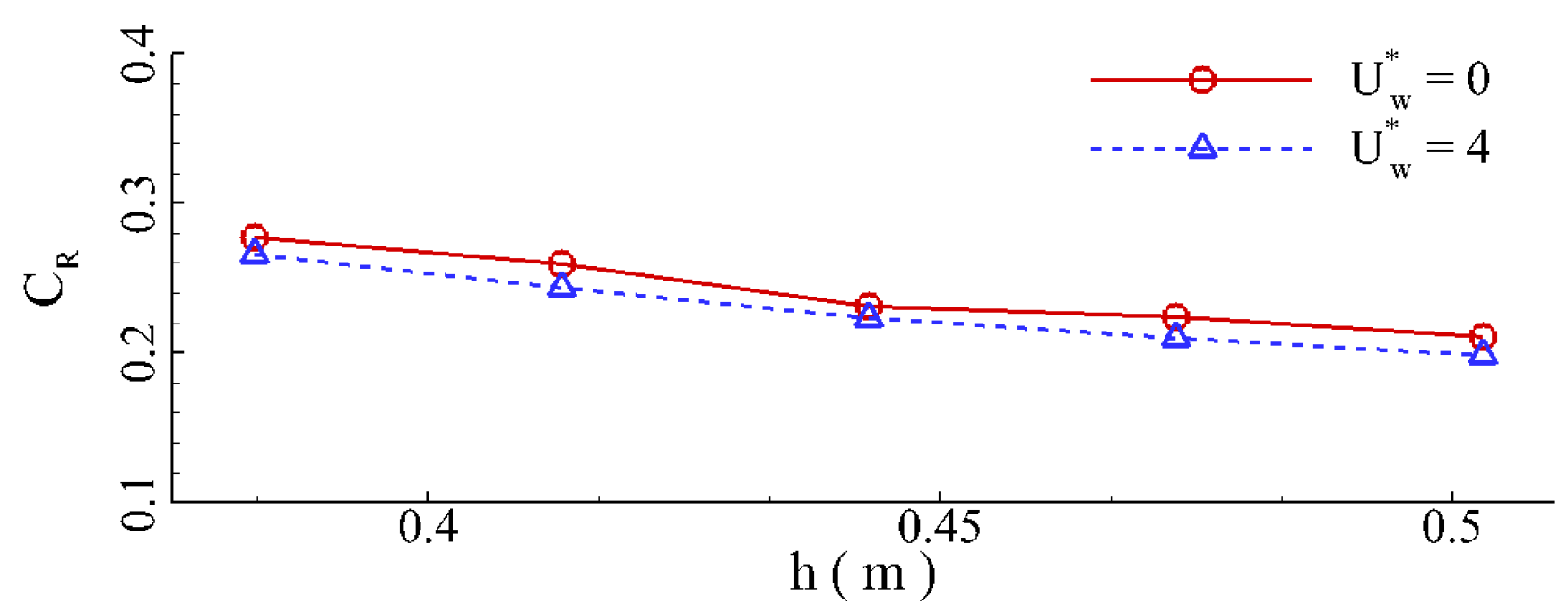
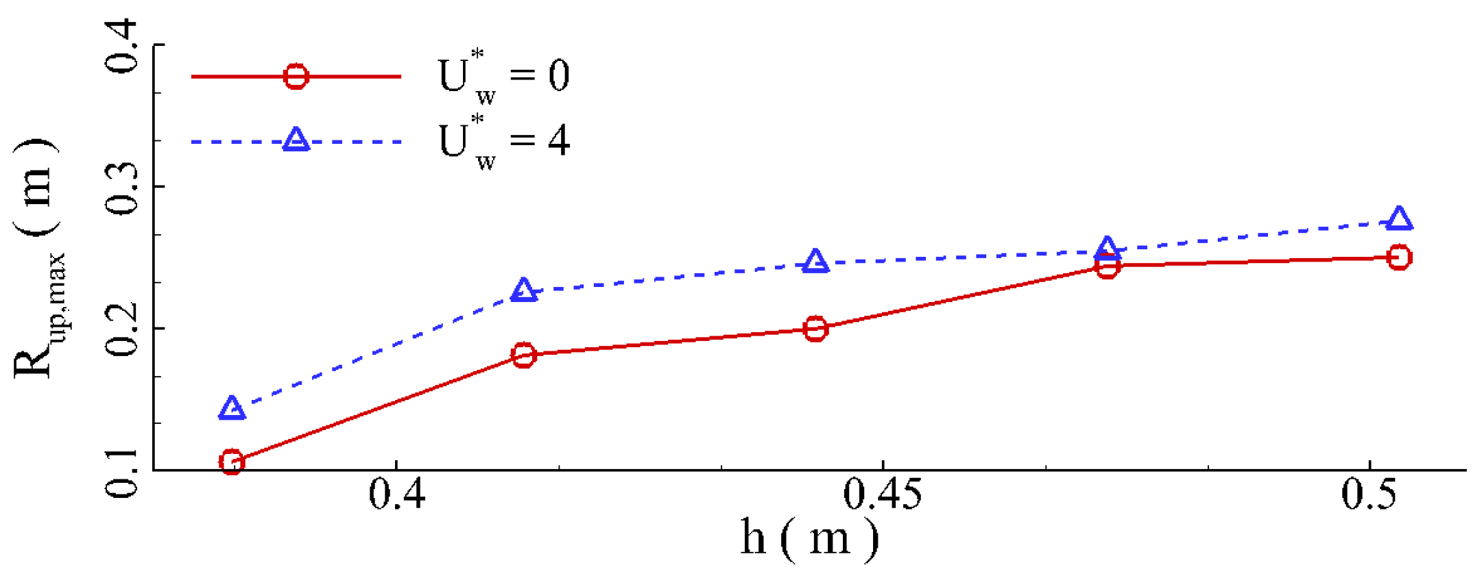
When the influences of the water depth on the hydrodynamics of solitary wave in the windy condition on the fringing reef are considered, five different water depths are chosen, i.e., $h$ = 0.383, 0.413, 0.443, 0.473 and 0.503 m, which produces five different submergence water depths, i.e., $h_r$ = 0, 0.03, 0.06, 0.09 and 0.12 m. The wave height ($H$) is kept as 0.11075 m. The spatial distributions of local wave height of solitary wave on the fringing reef under different water depths are depicted in Figure 19. As seen in Figure 19, when the reef flat is dry ($h$ = 0.383 m), the spatial distributions of the local wave heights of the solitary wave in the windy and no-wind conditions are nearly same (Figure 19a). When the water depth gradually increases, the differences in the local wave heights between the solitary wave in the windy and no-windy conditions gradually become larger after the wave breakings (Figure 19b,c). If the water depth ($h$) increases to 0.473 m, the differences in the local wave heights between the solitary wave in the windy and no-wind conditions become smaller again (Figure 19d). However, if the water depth is no less than 0.503 m, the spatial distributions of local wave heights exhibit a complex trend. The local wave heights after the wave breakings can become much greater than the incident wave height. Figure 20 plots the variations of wave reflection coefficients of the solitary wave on the fringing reef with the water depth. As depicted in Figure 20, the wave reflection coefficient of solitary wave tends to monotonically decrease with the water depth. It is attributed to the reason that when the water depth gradually increases, the blocking effects of the forereef slope on the solitary wave gradually decreases. When the water depth ($h$) increases from 0.383 m to 0.503 m, the wave reflection coefficient of solitary wave on the fringing reef decreases by 4.29% and 5.92% for the solitary wave in the windy and no-wind conditions, respectively. Figure 21 depicts the variation of the maximum value of wave runup height of solitary wave on the fringing reef with the water depth. Generally, the maximum value of wave runup height of solitary wave on the fringing reef gradually increases monotonically with the water depth. When the water depth ($h$) increases from 0.383 m to 0.503 m, the maximum value of wave runup height of solitary wave in the windy and no-windy conditions on the fringing reef increases by 33.8% and 10.25%, respectively. The maximum value of wave runup height of solitary wave in the windy condition is always greater than that in the no-wind condition, on average, 22.82% greater. However, when the water depth ($h$) is equal to 0.473 m, the difference in the maximum value of wave runup height between the solitary wave in the windy and no-wind conditions can be ignored.

4.4. Influences of Forereef and Backreef Slopes

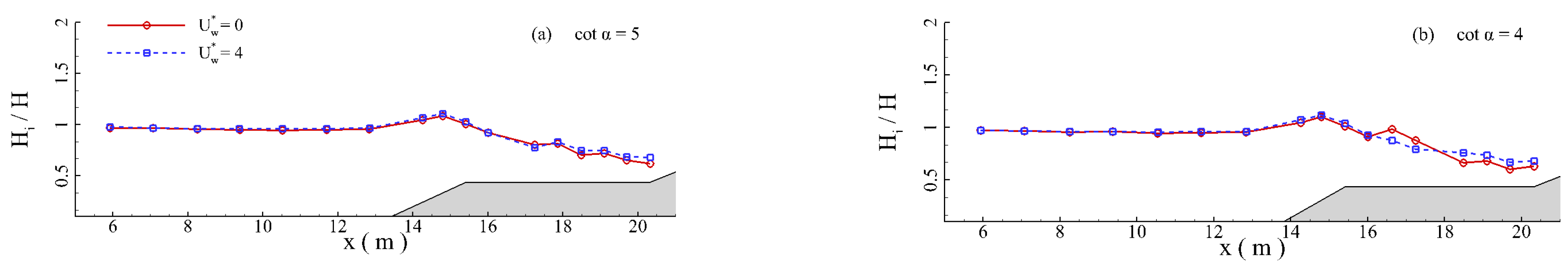
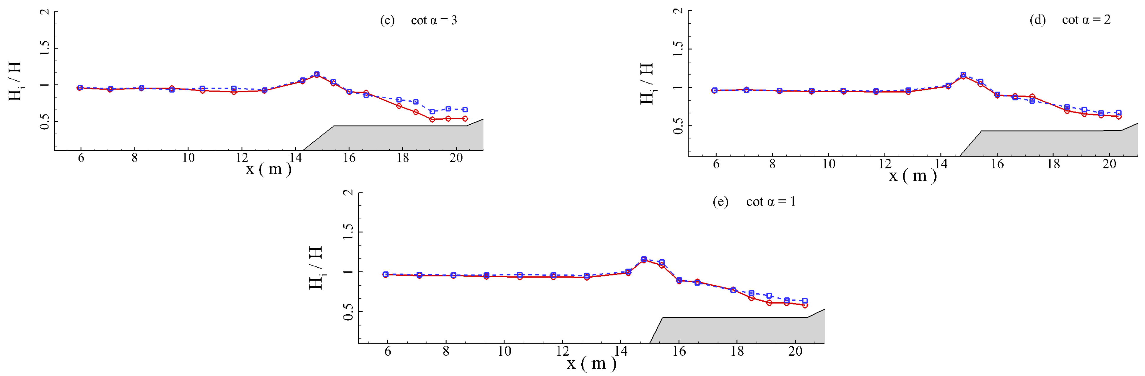
Influences of the forereef and backreef slopes on the hydrodynamic processes of solitary wave with the onshore wind on the fringing reef have been investigated in this section. The wave height ($H$) is 0.11075 m. The water depth ($h$) is 0.443 m. The dimensionless onshore wind speed ($U_w^{*}$) is set as 4. When the influences of forereef slope are considered, five different forereef slopes are chosen, i.e., $\cot \alpha$ = 5, 4, 3, 2 and 1. Figure 22 shows the spatial distributions of local wave height under different forereef slopes. It is shown that when the forereef slope is mild ($\cot \alpha$ = 5), the differences in the local wave heights between the solitary wave in the windy and no-wind conditions after the wave breakings can be ignored. When the forereef gradually increases from $\cot \alpha$ = 4 to $\cot \alpha$ = 3, the differences in the local wave height between the solitary wave in the windy and no-wind conditions after the wave breakings become more apparent. However, once the forereef slope becomes greater than $\cot \alpha$ = 2, the differences in the local wave heights between the solitary wave in the windy and no-windy conditions after the wave breakings tends to decrease gradually. Figure 23 depicts the variations of wave reflection coefficient with the forereef slope. As seen in Figure 23, the wave reflection coefficient almost increases linearly with the forereef slope. When the forereef slope increases from $\cot \alpha$ = 5 to $\cot \alpha$ = 1, the wave reflection coefficient increases by 11.02% and 5.12% for the solitary wave in the windy and no-wind conditions, respectively. Figure 24 plots the variations of maximum value of the wave runup height with the forereef slope. It clearly shows that the forereef slope can only slightly influence the maximum value of wave runup height, especially for the solitary wave in the windy condition. The maximum value of wave runup height of the solitary wave in the windy condition is, on average, 15.58% greater than that in no-wind condition.

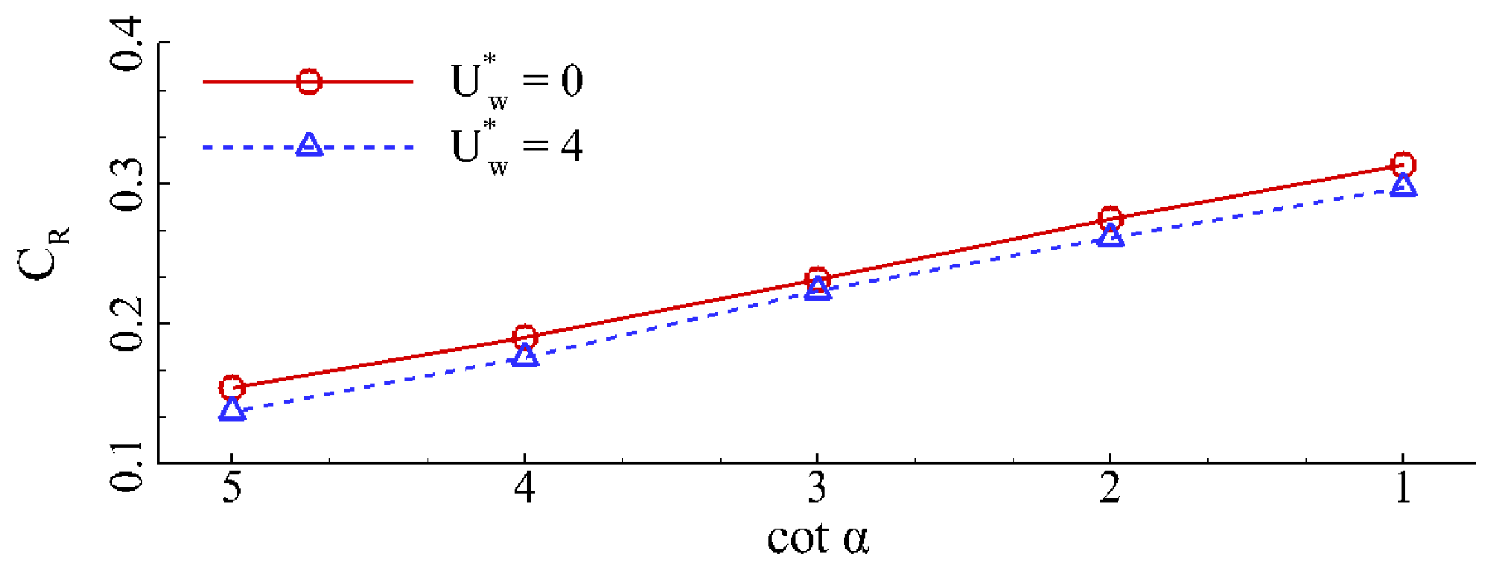
When the influences of backreef slope on the hydrodynamic processes of solitary wave with the onshore wind on the fringing reef are investigated, four different backreef slopes are chosen, i.e.,$\cot \beta$ = 20, 15, 10 and 5. Figure 25 shows the spatial distributions of local wave heights under different backreef slopes. The local wave heights of solitary wave in the windy condition are generally greater than that in no-wind condition ($x>$ 18 m) after the wave breaking processes. It is also observed that when the backreef slope is mild, the differences in the local wave heights between the solitary wave in the windy and no-wind conditions are very limited ($\cot \beta$ = 20), as seen in Figure 25a. As the backreef slope gradually increases from $\cot \beta$ = 15 to $\cot \beta$ = 5, the differences in the local wave heights between the solitary wave in the windy and no-wind conditions after the wave breakings tend to increase, especially at the toe of the backreef slope. Obviously, the variation of backreef slope has no noticeable influences on the wave reflection coefficient, as depicted in Figure 26. Figure 27 depicts the variation of the maximum value of wave runup height with the backreef slope. As seen in Figure 26, the maximum value of wave runup height monotonically increases with the backreef slope for both solitary wave with and without the onshore wind. As the backreef slope increases from $\cot \beta$ = 20 to $\cot \beta$ = 5, the maximum value of wave runup height increases by 13.81% and 10.27% for the solitary wave in the windy and no-windy conditions, respectively. Meanwhile, the maximum value of wave runup height of solitary wave in the windy condition is, on average, 15.49% greater than that in no-wind condition.

5. Conclusions

Based on a high-resolution two-phase wind-wave numerical tank, effects of the onshore wind on the hydrodynamics of solitary wave on the fringing reef have been investigated. Influences of several main factors are also discussed in detail. The main research findings of this study can be organized as:

(1)

The significant velocity differences between the water and air phases can produce a strong shear stress force at the water surface. In addition, when the strong onshore wind blows over the crest of solitary wave, low-pressure regions can be formed over the wave crest or the front side of breaking surge bore, resulting in strong pressure imbalances. Noticeable water surface oscillations can be observed, especially in the leeward region. Under the driving forces of the onshore wind, the breaking surge bore will produce a greater wave runup height. For the basic run, the maximum value of wave runup height of solitary wave under the action of onshore wind can be 22.6% greater than that without the wind;

(2)

As the wind speed continues to increase, the time of occurrence of wave breaking continues to advance. The wave reflection coefficient gradually decreases with the onshore wind speed. When the wind speed ($U_w^{*}$) increases from 0 to 6, the wave reflection coefficient decreases by 8.66%. This is attributed to the reason that the propagation celerity of solitary wave gradually increases under the increasingly intensified blowing effects of onshore wind. The maximum value of wave runup height of solitary wave increases linearly with the onshore wind speed. When the wind speed ($U_w^{*}$) increases from 0 to 6, the maximum wave runup height increases by 38.49%;

(3)

When the relative wave height ($H/h$) increases from 0.15 to 0.35, wave reflection coefficient of the solitary wave in the windy and no-windy conditions decreases by 8.92% and 1.94%, respectively. Meanwhile, the maximum value of wave runup height of the solitary wave in the windy and no-windy conditions increases by 10.95% and 13.98%, respectively. The maximum value of wave runup height of solitary wave in the windy condition is always larger than that of solitary wave in no-windy condition, averagely 16.67% larger;

(4)

As the water depth gradually increases, the wave reflection coefficient of solitary wave tends to decrease monotonically. It is attributed to the reason that an increase in the water depth can cause the blocking effects of the forereef slope on the solitary wave to decreases. As the water depth ($h$) increases from 0.383 m to 0.503 m, the wave reflection coefficient of solitary wave in the windy and no-windy conditions decreases by 4.29% and 5.92%, respectively. However, the maximum value of wave runup height of the solitary wave in the windy and no-windy conditions increases by 33.8% and 10.25%, respectively. The maximum value of wave runup height of the solitary wave in the windy condition is always greater than that in no-wind condition, on average, 22.82% greater;

(5)

When the forereef slope is mild, the differences in the spatial distributions of local wave heights after the wave breakings can be ignored. As the forereef slope ($\cot \alpha$) increases from 5 to 1, the wave reflection coefficient of solitary wave in the windy and no-windy conditions increases by 11.02% and 5.12%, respectively. However, the forereef slope can only slightly influence the maximum value of wave runup height, especially for the solitary wave in the windy condition. The maximum value of wave runup height of the solitary wave in the windy condition is, on average, 15.58% greater than that in the no-wind condition;

(6)

The variation of backreef slope has no noticeable influences on the wave reflection coefficient. The maximum value of wave runup height monotonically increases with the backreef slope for both solitary wave in the windy and no-wind conditions. As the backreef slope ($\cot \beta$) increases from 20 to 5, the maximum value of wave runup height of the solitary wave in the windy and no-wind conditions increases by 13.81% and 10.27%, respectively. Meanwhile, the maximum value of wave runup height of the solitary wave in the windy condition is, on average, 15.49% greater than that in the no-wind condition.

It is hoped that the research results of this study can enhance the understandings on the hydrodynamic characteristics of fringing reefs during extreme weather events.

References

- Gourlay, M.R.; Colleter, G. Wave-generated flow on coral reefs—An analysis for two-dimensional horizontal reef-tops with steep faces. Coast. Eng. 2005, 52, 353–387. [Google Scholar] [CrossRef]
- Li, Y.; Zhang, C.; Chen, D.; Zheng, J.; Sun, J.; Wang, P. Barred beach profile equilibrium investigated with a process-based numerical model. Cont. Shelf Res. 2021, 222, 104432. [Google Scholar] [CrossRef]
- Buckley, M.L.; Lowe, R.; Hansen, J.; Van Dongeren, A. Wave setup over a fringing reef with large bottom roughness. J. Phys. Oceanogr. 2016, 46, 2317–2333. [Google Scholar] [CrossRef]
- Baldock, T.E.; Shabani, B.; Callaghan, D.P.; Hu, Z.; Mumby, P.J. Two-dimensional modelling of wave dynamics and wave forces on fringing coral reefs. Coast. Eng. 2020, 155, 103594. [Google Scholar] [CrossRef]
- Lugo-Fernandez, A.; Roberts, H.H.; Suhayda, J.N. Wave transformations across a Caribbean fringing-barrier coral reef. Cont. Shelf Res. 1998, 18, 1099–1124. [Google Scholar] [CrossRef]
- Lowe, R.J.; Koseff, J.R.; Monismith, S.G. Oscillatory flow through submerged canopies: 1. Velocity structure. J. Geophys. Res. 2005, 110, C10016. [Google Scholar] [CrossRef] [Green Version]
- Yao, Y.; He, F.; Tang, Z.; Liu, Z. A study of tsunami-like solitary wave transformation and run-up over fringing reefs. Ocean Eng. 2018, 149, 142–155. [Google Scholar] [CrossRef]
- Gourlay, M.R. Wave transformation on a coral reef. Coast Eng. 1994, 23, 17–42. [Google Scholar] [CrossRef]
- Gourlay, M.R. Wave set-up on coral reefs. 2. Wave set-up on reefs with various Profiles. Coast Eng. 1996, 28, 17–55. [Google Scholar] [CrossRef]
- Ning, Y.; Liu, W.J.; Zhao, X.Z.; Zhang, Y.; Sun, Z. Study of irregular wave run-up over fringing reefs based on a shock-capturing boussinesq model. Appl. Ocean Res. 2019, 84, 216–224. [Google Scholar] [CrossRef]
- Yao, Y.; Zhang, Q.; Chen, S.; Tang, Z. Effects of reef morphology variations on wave processes over fringing reefs. Appl. Ocean. Res. 2019, 82, 52–62. [Google Scholar] [CrossRef]
- Seelig, W.N. Laboratory study of reef-lagoon system hydraulics. J. Waterw. Port. Coast. Ocean Eng. 1983, 109, 380–391. [Google Scholar] [CrossRef]
- Buckley, M.L.; Lowe, R.; Hansen, J.; Van Dongeren, A. Dynamics of wave setup over a steeply sloping fringing reef. J. Phys. Oceanogr. 2015, 45, 150923131654000. [Google Scholar] [CrossRef] [Green Version]
- Demirbilek, Z.; Nwogu, O.G.; Ward, D.L. Laboratory Study of Wind Effect on Runup over Fringing Reefs, Report 1: Data Report; Coastal and Hydraulics Laboratory Technical Report ERDC/CHL-TR-07-4; U.S. Army Engineer Research and Development Center: Vicksburg, MS, USA, 2007. [Google Scholar]
- Becker, J.M.; Merrifield, M.A.; Yoon, H. Infragravity waves on fringing reefs in the tropical Pacific: Dynamic setup. J. Geophys. Res. Oceans. 2016, 121, 3010–3028. [Google Scholar] [CrossRef]
- Longuet-Higgins, M.S.; Stewart, R.W. Radiation stresses in water waves; a physical discussion, with applications. Deep. Sea. Res. Oceanogr. Abstr. 1964, 11, 529–562. [Google Scholar] [CrossRef]
- Fernando, H.; Samarawickrama, S.; Balasubramanian, S.; Hettiarachchi, S.; Voropayev, S. Balasubramanian, S. Effects of porous barriers such as coral reefs on coastal wave propagation. J. Hydro. Environ. Res. 2008, 1, 187–194. [Google Scholar] [CrossRef]
- Kunkel, C.; Hallberg, R.; Oppenheimer, M. Coral Reefs reduce tsunami impact in model simulations. Geophys. Res. Lett. 2006, 33, L23612. [Google Scholar] [CrossRef] [Green Version]
- Lynett, P.J. Effect of a shallow water obstruction on long wave runup and overland flow velocity. J. Waterw. Port Coast. Ocean. Eng. 2007, 133, 455–462. [Google Scholar] [CrossRef] [Green Version]
- Ma, G.; Su, S.-F.; Liu, S.; Chu, J.-C. Numerical simulation of infragravity waves in fringing reefs using a shock-capturing non-hydrostatic model. Ocean. Eng. 2014, 85, 54–64. [Google Scholar] [CrossRef]
- Nwogu, O.; Demirbilek, Z. Infragravity wave motions and run-up over shallow fringing reefs. J. Waterw. Port Coast. Ocean Eng. 2010, 136, 295–305. [Google Scholar] [CrossRef]
- Péquignet, A.C.N.; Becker, J.M.; Merrifield, M.A.; Aucan, J. Forcing of resonant modes on a fringing reef during tropical storm Man-Yi. Geophys. Res. Lett. 2009, 36, L03607. [Google Scholar] [CrossRef] [Green Version]
- Gawehn, M.; van Dongeren, A.; van Rooijen, A.; Storlazzi, C.D.; Cheriton, O.M.; Reniers, A. Identification and classification of very low frequency waves on a coral reef flat. J. Geophys. Res. Oceans. 2016, 121, 7560–7574. [Google Scholar] [CrossRef] [Green Version]
- Qu, K.; Ren, X.Y.; Kraatz, S. Numerical investigation of tsunami-like wave hydrodynamic characteristics and its comparison with solitary wave. Appl. Ocean Res. 2017, 63, 36–78. [Google Scholar] [CrossRef]
- Ford, M.R.; Becker, J.M.; Merrifield, M.A. Reef flat wave processes and excavation pits: Observations and implications for Majuro Atoll, Marshall Islands. J. Coast Res. 2013, 29, 545–554. [Google Scholar] [CrossRef]
- Goda, Y. Derivation of unified wave overtopping formulae for seawalls with smooth, impermeable surfaces based on selected CLASH datasets. Coast. Eng. 2009, 56, 385–399. [Google Scholar] [CrossRef]
- Shao, K.; Liu, W.; Gao, Y.; Ning, Y. The influence of climate change on tsunami-like solitary wave inundation over fringing reefs. J. Integr. Environ. Sci. 2019, 16, 17–88. [Google Scholar] [CrossRef] [Green Version]
- Roeber, V.; Cheung, K.F.; Kobayashi, M.H. Shock-capturing Boussinesq-type model for nearshore wave processes. Coast. Eng. 2010, 57, 407–423. [Google Scholar] [CrossRef]
- Roeber, V.; Cheung, K.F. Boussinesq-type model for energetic breaking waves in fringing reef environments. Coast. Eng. 2012, 70, 1–20. [Google Scholar] [CrossRef]
- Kazolea, M.; Filippini, A.; Ricchiuto, M.; Abadie, S.; Medina, M.M.; Morichon, D.; Journeau, C.; Marcer, R.; Pons, K.; LeRoy, S.; et al. Wave propagation, breaking, and overtopping on a 2D reef: A comparative evaluation of numerical codes for tsunami modelling. Eur. J. Mech. B-fluid. 2019, 73, 122–131. [Google Scholar] [CrossRef] [Green Version]
- Quiroga, P.D.; Cheung, K.F. Laboratory study of solitary-wave transformation over bed-form roughness on fringing reefs. Coast. Eng. 2013, 80, 35–48. [Google Scholar] [CrossRef]
- Liu, W.; Shao, K.; Ning, Y. A study of the maximum momentum flux in the solitary wave run-up zone over back-reef slopes based on a boussinesq model. J. Mar. Sci. Eng. 2019, 7, 109. [Google Scholar] [CrossRef] [Green Version]
- Qu, K.; Liu, T.W.; Chen, L.; Yao, Y.; Kraatz, S.; Huang, J.X.; Lan, G.Y.; Jiang, C.B. Study on transformation and runup processes of tsunami-like wave over permeable fringing reef using a nonhydrostatic numerical wave model. Ocean Eng. 2022, 243, 110228. [Google Scholar] [CrossRef]
- Jeffreys, H. On the formation of water waves by wind. Proc. R. Soc. Lond. Ser. A Math. Phys. Eng. Sci. 1925, 107, 189–206. [Google Scholar]
- Miles J, W. On the generation of surface waves by shear flows. J. Fluid Mech. 1957, 3, 185–204. [Google Scholar] [CrossRef]
- Banner, M.L.; Melville, W.K. On the separation of air flow over water waves. J. Fluid Mech. 1976, 77, 825–842. [Google Scholar] [CrossRef] [Green Version]
- Douglass, S.L.; Weggel, J.R. Laboratory experiments on the influence of wind on nearshore wave breaking. Coast. Eng. Proc. 1988, 21, 46. [Google Scholar] [CrossRef] [Green Version]
- Sous, D.; Forsberg, P.L.; Touboul, J.; Nogueira, G.G. Laboratory experiments of surf zone dynamics under on-and offshore wind conditions. Coast. Eng. 2021, 163, 103797. [Google Scholar] [CrossRef]
- King, D.M.; Baker, C.J. Changes to wave parameters in the surf zone due to wind effects. J. Hydraul Res. 1996, 34, 55–76. [Google Scholar] [CrossRef]
- Liu, X. A laboratory study of spilling breakers in the presence of light-wind and surfactants. J. Geophys Res-Oceans. 2016, 121, 1846–1865. [Google Scholar] [CrossRef]
- Touboul, J.; Giovanangeli, J.P.; Kharif, C. Freak waves under the action of wind: Experiments and simulations. Eur. J. Mech. B-fluid. 2006, 25, 662–676. [Google Scholar] [CrossRef]
- Tian, Z.; Choi, W. Evolution of deep-water waves under wind forcing and wave breaking effects: Numerical simulations and experimental assessment. Eur. J. Mech. B-fluid. 2013, 41, 11–22. [Google Scholar] [CrossRef]
- Yan, S.; Ma, Q.W. Numerical simulation of interaction between wind and 2D freak waves. Eur. J. Mech. B-fluid. 2010, 29, 18–31. [Google Scholar] [CrossRef] [Green Version]
- Marino, E.; Borri, C.; Lugni, C. Influence of wind–waves energy transfer on the impulsive hydrodynamic loads acting on offshore wind turbines. J. Wind Eng. Ind. Aerod. 2011, 99, 767–775. [Google Scholar] [CrossRef]
- Zou, Q.; Chen, H. Wind and current effects on extreme wave formation and breaking. J. Phys. Oceanogr. 2017, 47, 1817–1841. [Google Scholar] [CrossRef]
- Hieu, P.D.; Vinh, P.N.; Son, N.T. Study of wave–wind interaction at a seawall using a numerical wave channel. Appl. Math. Mode. 2014, 38, 5149–5159. [Google Scholar] [CrossRef]
- Qu, K.; Wen, B.; Ren, X.; Kraatz, S.; Sun, W.; Deng, B.; Jiang, C. Numerical investigation on hydrodynamic load of coastal bridge deck under joint action of solitary wave and wind. Ocean Eng. 2020, 217, 108037. [Google Scholar] [CrossRef]
- Wen, B.H.; Qu, K.; Lan, G.Y.; Sun, W.Y.; Yao, Y.; Deng, B.; Jiang, C.B. Numerical study on hydrodynamic characteristics of coastal bridge deck under joint action of regular waves and wind. Ocean Eng. 2022, 245, 110450. [Google Scholar] [CrossRef]
- Fergizer, J.; Peric, M. Computational Methods for Fluid Dynamics; Springer: Berlin/Heidelberg, Germany, 2002. [Google Scholar]
- Jasak, H. Error Analysis and Estimation for the Finite Volume Method with Applications to Fluid Flows. Ph.D. Dissertation, University of London, London, UK, 1996. [Google Scholar]
- Rhie, C.; Chow, W. A Numerical Study of the Turbulent Flow Past an Isolated Airfoil with Trailing Edge Separation. In Proceedings of the 3rd Joint Thermophysics, Fluids, Plasma and Heat Transfer Conference, Fluid Dynamics and Co-located Conferences, St. Louis, MO, USA, 7–11 June 1982. [Google Scholar]
- Issa, R. Solution of the implicitly discretized fluid flow equations by operator splitting. J. Comput. Phys. 1986, 62, 40–65. [Google Scholar] [CrossRef]
- Wilcox, D.C. Turbulence Modeling for CFD; DCW Industries Inc.: La Canada, CA, USA, 1994. [Google Scholar]
- Darwish, M.; Moukalled, F. Convective schemes for capturing interfaces of free surface flow on unstructured grids. Num. Heat Transf. B-Fund. 2006, 49, 19–42. [Google Scholar] [CrossRef]
- Willmott, C.J. On the Validation of Models. Phys. Geogr. 1981, 2, 184–194. [Google Scholar] [CrossRef]
Figure 1.
Experimental layout.
Figure 2.
Time series of the water elevations at different wave gauges; (a) WG1; (b) WG2; (c) WG3; (d) WG4; (e) WG5; (f) WG6.
Figure 3.
Time series of the wave runup height.
Figure 4.
Computational layout.
Figure 5.
Plots of water velocity contour at different time moments: left side, without onshore wind; right side, with onshore wind; (a,b), t = 7 s; (c,d), t = 8 s; (e,f), t = 9 s; (g,h), t = 12 s.
Figure 6.
Plots of pressure contours of the water body at different time moments: left side (a,c), without onshore wind; right side (b,d), with onshore wind.
Figure 7.
Plots of the vector velocity field; left side shaded by the vorticity contour: left side, without onshore wind; right side, with onshore wind.
Figure 8.
The shear stress contours during wave breaking; left side, without onshore wind; right side, with onshore wind.
Figure 9.
Time series of the water elevation at different wave gauges; (a) WG1; (b) WG10; (c) WG15; (d) WG18.
Figure 10.
Spatial distributions of the local wave height.
Figure 11.
Figure 12.
Plots of water velocity contours at different time moments under different wind speed. (a,b), = 0; (c,d), = 2; (e,f), = 4; (g,h), = 6.
Figure 13.
Spatial distributions of the local wave heights under different wind speeds.
Figure 14.
Variations of the wave reflection coefficients with the wind speed.
Figure 15.
Variations of the maximum values of wave runup height with the wind speed.
Figure 16.
Spatial distributions of the local wave heights under different relative wave heights; (a) = 0.15; (b) = 0.2; (c) = 0.25; (d) = 0.3; (e) = 0.35.
Figure 17.
Variations of the wave reflection coefficient with the relative wave height.
Figure 18.
Variations of the maximum value of wave runup height with the relative wave height.
Figure 19.
Spatial distributions of local wave height under different water depths; (a) = 0.383 m; (b) = 0.413 m; (c) = 0.443 m; (d) = 0.473 m; (e) = 0.503 m.
Figure 20.
Variation of the wave reflection coefficient with the water depth.
Figure 21.
Variation of the maximum values of wave runup height with the water depth.
Figure 22.
Spatial distributions of the local wave heights under different forereef slopes; (a) = 5; (b) = 4; (c) = 3; (d) = 2; (e) = 1.
Figure 23.
Variation of the wave reflection coefficient with the forereef slope.
Figure 24.
Variation of the maximum values of wave runup height with the forereef slope.
Figure 25.
Spatial distributions of the local wave heights under different backreef slopes; (a) = 20; (b) = 15; (c) = 10; (d) = 5.
Figure 26.
Variation of the wave reflection coefficient with the backreef slope.
Figure 27.
Variation of the maximum values of wave runup height with the backreef slope.
Publisher’s Note: MDPI stays neutral with regard to jurisdictional claims in published maps and institutional affiliations. |
© 2022 by the authors. Licensee MDPI, Basel, Switzerland. This article is an open access article distributed under the terms and conditions of the Creative Commons Attribution (CC BY) license (https://creativecommons.org/licenses/by/4.0/).
Share and Cite
MDPI and ACS Style
Guo, L.; Qu, K.; Huang, J.X.; Li, X.H. Numerical Study of Influences of Onshore Wind on Hydrodynamic Processes of Solitary Wave over Fringing Reef. J. Mar. Sci. Eng. 2022, 10, 1645. https://doi.org/10.3390/jmse10111645
AMA Style
Guo L, Qu K, Huang JX, Li XH. Numerical Study of Influences of Onshore Wind on Hydrodynamic Processes of Solitary Wave over Fringing Reef. Journal of Marine Science and Engineering. 2022; 10(11):1645. https://doi.org/10.3390/jmse10111645
Chicago/Turabian StyleGuo, L., K. Qu, J. X. Huang, and X. H. Li. 2022. "Numerical Study of Influences of Onshore Wind on Hydrodynamic Processes of Solitary Wave over Fringing Reef" Journal of Marine Science and Engineering 10, no. 11: 1645. https://doi.org/10.3390/jmse10111645
Note that from the first issue of 2016, this journal uses article numbers instead of page numbers. See further details here.