Surface Waves Prediction Based on Long-Range Acoustic Backscattering in a Mid-Frequency Range

Abstract

Underwater acoustic echosounding for surface roughness parameters retrieval is studied in a frequency band that is relatively new for such purposes. During the described 2-weeks sea experiment, 1–3 kHz tonal pulses were emitted from an oceanographic platform, located on the northern Black Sea shelf. Doppler spectra of the resulting reverberation were studied. The frequency band of the acoustic system, selected for this study, is chosen due to the fact that the sound propagation range is large enough for remote sensing in a coastal zone, and the resolution cell size does not limit the research. Backscattering of acoustical signals was received for distances around two nautical miles. However, it turned to be quite difficult to interpret the obtained data since backscattering spectrum shape was influenced by a series of effects, resulting in a complicated link to wind waves and currents’ parameters. Significant wave height and dominant wave frequency were estimated as the result of such signals processed with the use of machine learning tools. A decision-tree-based mathematical regression model was trained to solve the inverse problem. Wind waves prediction is in a good agreement with direct measurements, made on the platform, and machine learning results allow physical interpretation.

1. Introduction

Monitoring and forecasting of currents and wind waves is necessary for activities such as ship navigation, and routine operation of ports and offshore platforms. Studies in different areas of ocean physics rely on statistics of long-term observations. Different methods and instruments are used to do such measurements and collected data might be used, for example, to validate models and to assimilate data in real-time forecasting [1,2].

A huge amount of remote measurements tasks in the sea are fulfilled with the use of radars and other microwave instruments. The methods of extracting the period and direction of the waves from the radar data are well-developed [3]. The possibility of measuring the wave height based on the data on the backscattering intensity has been studied in a number of papers, e.g., in [4]. In contrast to the backscattering intensity, the usage of Doppler frequency shift of the reflected radio wave can be treated as a direct form of measurement since it is associated with the orbital velocities of the wind waves. This is the principle underlying operation of a radar device used to determine wave heights [5]. The possibility of determining the wave height and surface currents using coherent radar data at a low grazing angle was studied in [6,7,8,9]. It has been shown that the wave spectra and currents reconstructed from velocity radar images correlate with the data of contact measurements, both qualitatively and quantitatively.

For many reasons, the usage of acoustic measurement tools is attractive too. Acoustic Doppler current profiler (ADCP) is a very widely-used tool to measure speed in a water column, and modern models are facilitated with a function to measure surface waves spectra as well [10]. ADCP is equipped with 4 echo sounder beams that can be treated as four water height gauges that allow tracking elevation and skew of the surface, produced by long waves. Another design of upward-looking acoustic tools relies on a sound scattering model to reconstruct surface spectrum moments based on the Doppler spectrum of the reflected signal [11,12,13].

High frequency signal reverberation patterns may allow for tracking individual wave crests in vicinity of the transducer, as it has been reported by [14,15]. The mentioned tools are designed for local measurements and methods to assess waves and currents on a long range are of great interest too. The coastal acoustic tomography technique allows the estimation of mean current in a channel or a strait basing on acoustic pulses travel times between multiple sources and receivers, organized in a net. The recent papers [16,17,18] showed great progress in that. A group of bottom-mounted transmitter—receivers can also allow for track passage of internal waves through such a field of sensors [19].

An acoustic environmental monitoring system can be designed analogous to a radar. Underwater sound scattering on surface roughness is very much analogous to microwave scattering. Under similar conditions, acoustic scattering strength matches the one for microwaves until bubbles start to appear in a large amount [20]. When one takes grazing angles, underwater sound propagation is not limited by direct line of sight due to the waveguide effects. Compact devices can transmit sound pulses of the frequency of several kilohertz that will travel several kilometers. Long-range reverberation is a result of averaged interaction of sound with surface waves, so that scattering intensity is accumulated over a large patch of the surface: around ten surface wavelengths in diameter or larger.

Small perturbation theory (SPT) gives a rather straightforward relation between the power spectral density (PSD) of the scattered signal and surface waves PSD due to Bragg resonance of sound waves with surface waves [21,22]. A measurement method was proposed by [23], but the realization of that routine was not reported. The authors of [24] presented the experimental data as up-Bragg and down-Bragg levels and showed that the direction of the most intensive scattering signal arrival is correlated with the wind direction. However, a spectrum of the scattered signal was not shown in that paper. Prior to that scattering strength (SS), Ref. [25] was related to a wind speed, a frequency and other parameters by Chapman and Harris curve [22,25], which is an empirical function that partly mismatches with the SPT results.

SPT-based models are not detailed if the sea surface is too rough in comparison with the sound wavelength or the bubbles that are not included into model appear in large amounts. It was noticed [26] that the backscattering level differs from the one predicted by linear theory, starting from the wind speed 7–10 m/s and frequency of 300–500 Hz. This is called anomalous low frequency surface reverberation. The phenomenon is explained by scattering on cavities and bubble clouds, which appear due to wave breaking [27]. Such clouds may contain a measurable amount of bubbles of 1–3 mm diameter [28], and those may have an influence on sound propagation and scattering in the band around 1 kHz [29,30]. For this reason, how the presence of bubble is revealed in the scattering of Doppler-sensitive signals has been studied [31]. We showed that the bubble scattering has a specific signature in backscattering Doppler spectra. Subsurface bubbles move definitely slower than typical phase speeds of wave crests. They are carried by oscillating wind-waves-driven currents as well as by the mean water currents in the upper layer.

Doppler surface scattering prediction in the 1–3 kHz band is often studied in the context of sonar performance modeling [32,33,34]. The present research is devoted to the inverse problem of predicting a sea surface state based on a backscattering signal. What we are going to analyze here is actually the reverberation signal.

To test the possibility of reconstruction of such parameters, a continuous complex experiment was carried out. A sonar, made of researchers’ equipment and based on a sea platform, was working in the same regime during 14 days of the experiment, while the weather conditions varied. The experiment took place in the shelf zone of the northern part of the Black Sea in the second half of September 2021. All necessary parameters, concerning wind, waves and currents, were recorded in parallel with direct measurement tools. An acoustic signal processing algorithm was developed, and it included adjustable parameters to reconstruct the sea surface state. First, we tried adjust correlations manually, seeking correlation between input and output parameters and making calibration curves. Second, we found more practical to apply machine learning methods to do this. An Extreme Gradient Boosting (XGBoost) method, based on decision trees [35], was used for that. To make it applicable, part of the data (random time intervals) was treated as a training dataset, and the rest was used for testing.

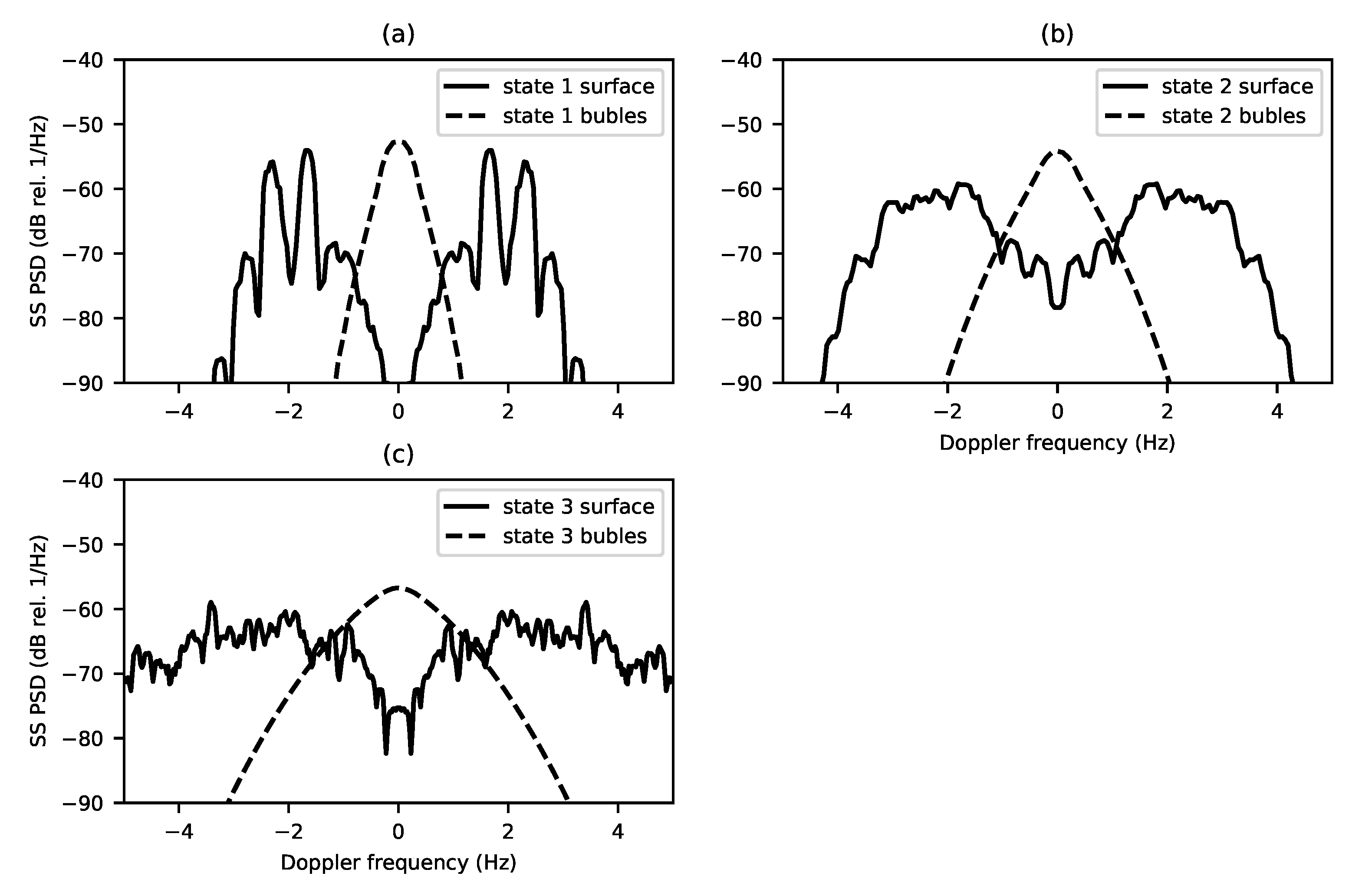
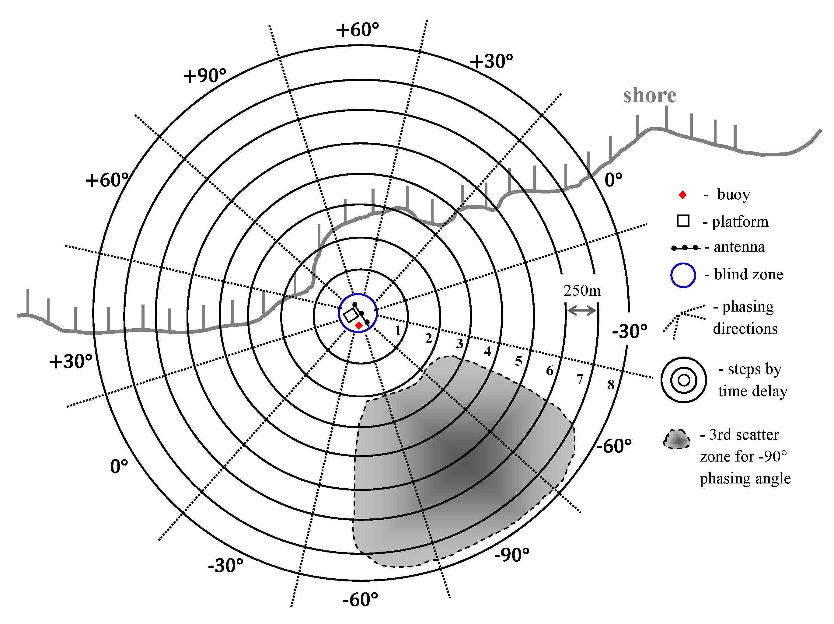
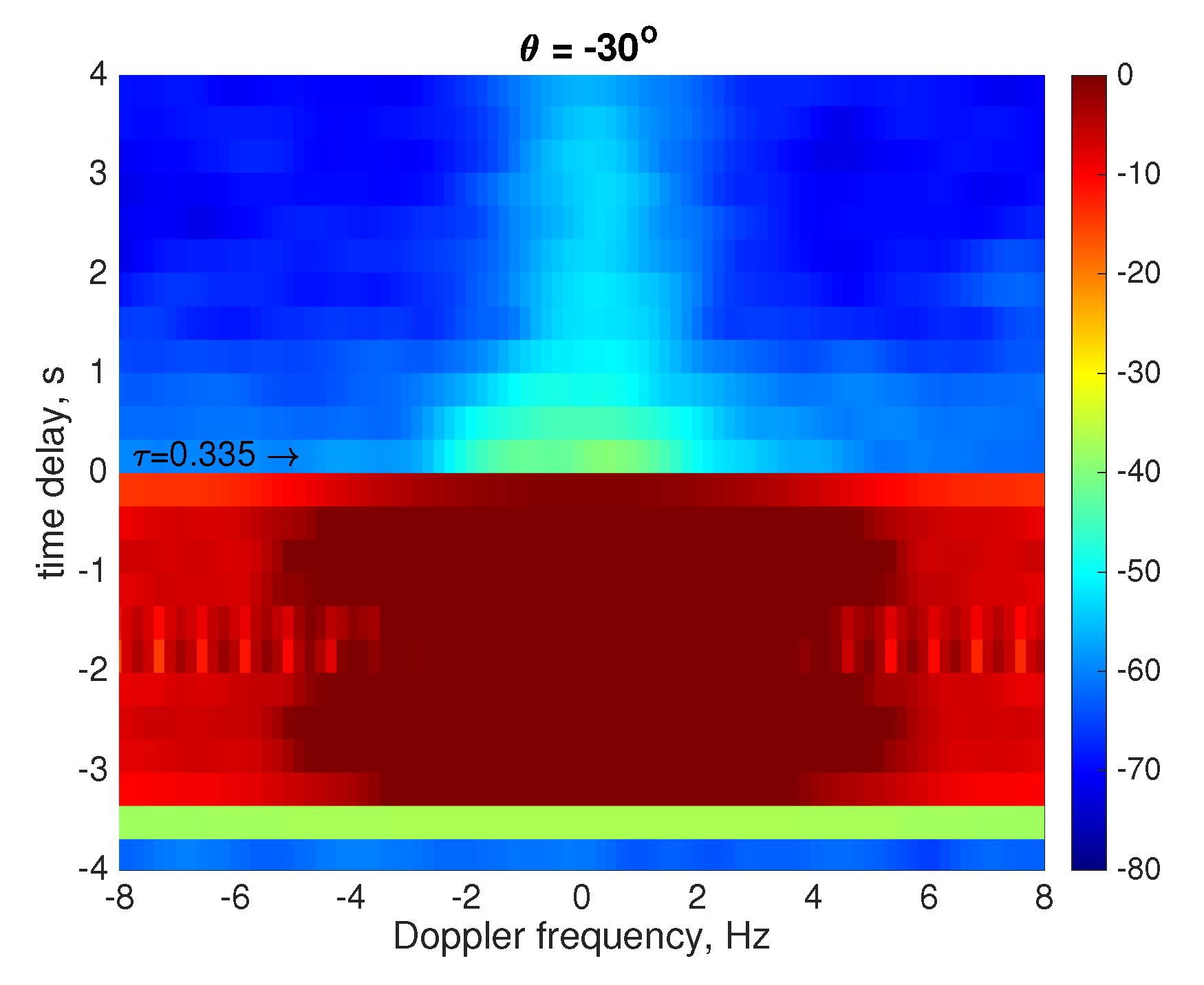
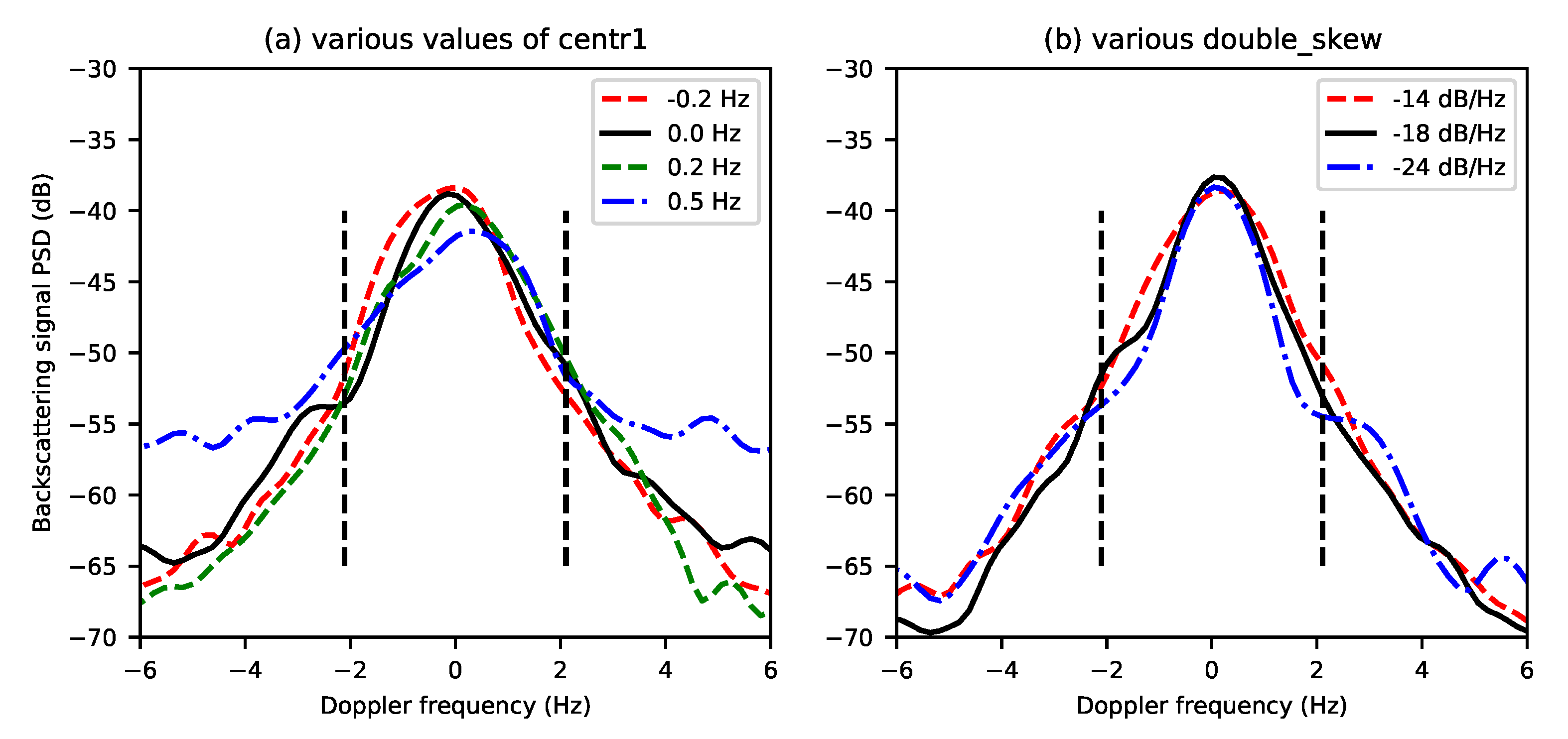
2. Theory Background

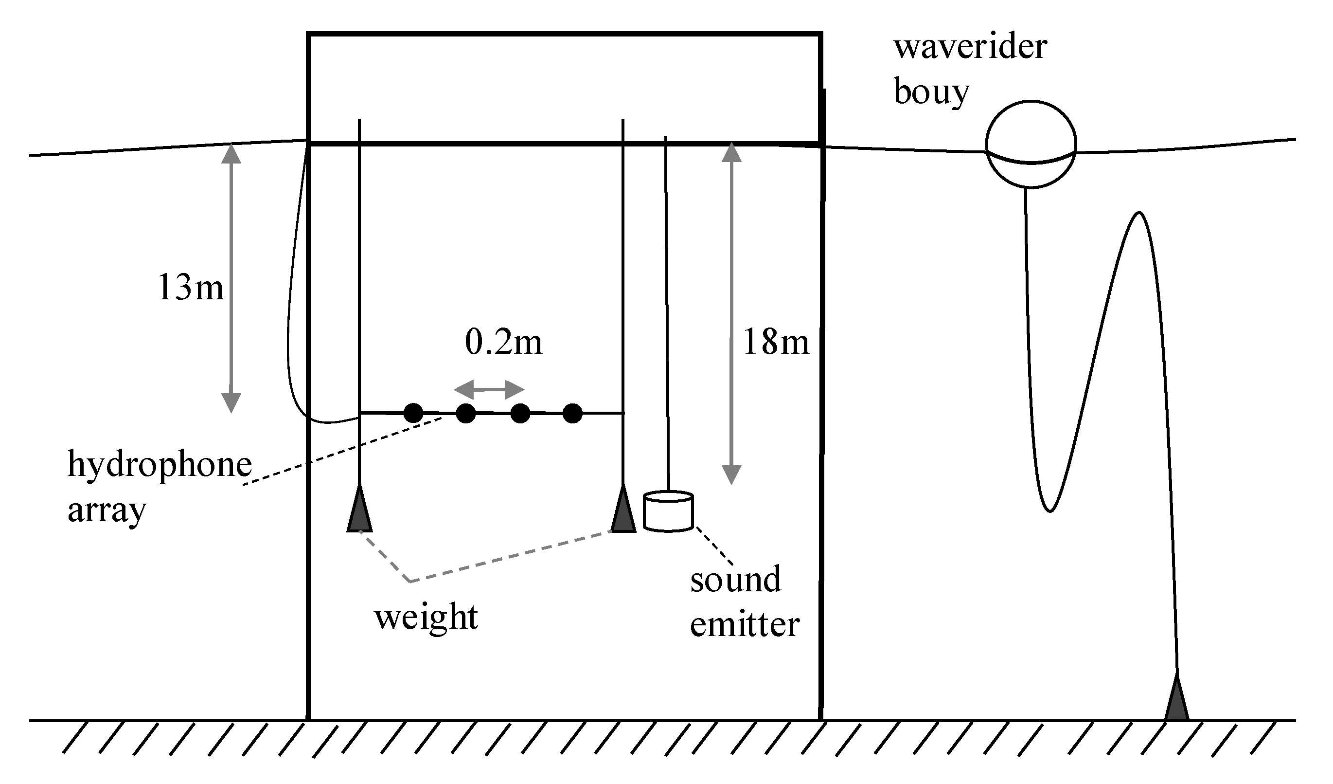
To understand the sound scattering phenomenon in this experiment, one should keep in mind that the rough surface is personified not only by the direct arrival, but by the sound waves, propagating by various paths with surface and bottom reflections. Although sophisticated methods of computing reverberation in a shallow water waveguide exist [36,37], in practice, we may still rely on the sonar equation for overall estimates [22,25,38]. The model is the following. A sound wave experience many quasi-mirror reflections i.e., when the surface and the bottom are considered to be flat, preserving their mean levels. Each time, a small part of the energy is scattered backward (and this part is too small to account for extra decay of the forward propagating wave). Back propagation of scattered waves is modeled so that only quasi-mirror reflections are taken into account. Scattered signals reach the receiver with random phases, so only accumulations of intensities are needed.

Since all properties that define propagation remain stable during the experiment, all changes in scattering levels due to weather conditions should be linked to the SS parameter. A strong contribution of bottom scattering is expected in shallow water, so a level of Doppler side lobes in the spectrum of the scattering signal (i.e., PSD of SS) is going to be more reliable than total SS alone. Small perturbation theory might have help with theoretical analysis of such features, but it is valid in case the Rayleigh condition is satisfied:

$$P_R=2k{a}_{std}sin\left({\chi }_{☆}\right)<<1$$

(1)

where k is the acoustic wavenumber, $a_{std}$ is a root mean square of surface elevation, and ${\chi }_{☆}\approx {30}^{\circ }$ is a waveguide capture angle (that stands here because it is an estimate for the maximum grazing angle of an incident wave). The value of $a_{std}$ is related to a more common oceanography parameter, a significant wave height as $H_{m0}=4a_{std}$. Treating ‘much less’ as ‘equivalent with coefficient 0.16’ allows for concluding that, at the frequency of 1.5 kHz, small perturbation theory is valid up to $H_{m0}=10$ cm. Unfortunately, such low amplitude was observed only once during a half-hour session of the whole 2-week experiment.

Moreover, the $k-\omega$ spectrum of surface waves is known to diverge from its trivial form like:

$$G^2(\mathbf{K},\Omega )\approx \frac{g^2}{4\pi {\Omega }^3}S(\Omega )\delta \left(\Omega -\sqrt{gK}\right)\Phi (\varphi ,\Omega )$$

(2)

where $\mathbf{K}$ and $\Omega$ are a wave vector and a cyclic frequency of a surface wave, g is the acceleration due to gravity, $\varphi$ is the azimuth of K, and $\Phi$ is the angular spreading, normalized as follows: ${\int }_0^{2pi}\Phi (\varphi )d\varphi =2\pi$. Equation (2) is implicitly or explicitly used in many papers on low frequency scattering since the surface waves PSD $S(\Omega )$ as a function of frequency is much better studied than the 3D spectrum and linear dispersion law is assumed to be valid:

$${\Omega }^2=gK$$

(3)

To obtain some theoretical data on backscattering spectra, valid for the conditions of the experiment, the authors carried out a numerical simulation in the previous study [39]. The model was capable of accounting for both sound scattering in case of large surface displacements and for nonlinearity of surface waves. The results, reproduced from [39], are shown with solid lines on Figure 1 for different sea states. (Dashed curves in the same figure are going to be discussed later.) Remember that the exploited numerical model was 2D and thus proper calculation of scattering cross-section in area units was not possible. To make the results somehow correlate with the present study, we apply such kind of normalization that integration over frequency of any of the plotted curves will result in SS = −55 dB, which is a typical value [21,25].

The curve, labeled ‘state 1 surface’, shows approximately what we expect to obtain in terms of linear theory for sound scattering on the air—water interface because $P_r=0.08$ in this case. One can clearly see side lobes at Doppler frequencies of $\pm 1.6$ Hz, which are expected due to the Bragg effect. Taking into account this effect, the dispersion relation (3) and neglecting a vertical angle of incidence one may derive a common rule for their positions:

$$f_{Bragg}=\frac{\sqrt{2gk}}{2\pi }$$

(4)

Some distortions of the spectrum have already appeared in this state and side lobes are widened and blurred in state 2 so that no maximum can be observed in state 3. Moreover, one can see from the plots that the center of mass for each lobe tends to move to higher frequency (by absolute value) with the wave height increase.

The next effect that should be accounted for is bubble scattering. First, they are moved by the mean water flow (mainly near-surface flow) that creates constant Doppler shift. This results in the shift of the Doppler centroid. Second, they are moved by an oscillating field of currents, produced by surface waves. This creates double-side Doppler spreading with the dispersion proportional to the dispersion of the velocity:

$$v_{std}^2=\int {\Omega }^{2}S(\Omega )d\Omega$$

(5)

In most cases, $v_{std}$ increases with the increase of $H_{m0}$.

To obtain the shape of backscattering spectrum, created by subsurface bubble clouds, we use a computation routine, proposed in [31]. The simulation results are plotted by dashed lines in Figure 1. Some parameters are not known for that model. No actual concentration of bubbles is used for the computation. Instead of that, the resulting distribution is normalized to a total level of SS = −55 dB, as above. Next, bubble concentration is assumed exponentially decaying with a depth with e-times decay scale of 3 m, just as an example. As one can see from the plot, bubble oscillations due to surface waves currents are expected to create triangle-shaped spectra with not very high Doppler frequencies. As waves height increases, Doppler spreading increases too.

The resulting idea is that we actually have two concurrent models, which are scattering on surface waves, accounting for their nonlinearity, and scattering on subsurface bubbles that are driven by currents. Whichever of them is dominant, the following behavior of output parameters is expected. Water flux results in the shift of the Doppler spectrum centroid. Increase in significant wave height results in increase of the spectral width. The listed effects are local, and we may use beamforming in the horizontal plane and time delay to probe the surrounding water area.

3. Materials

The experiment took place on an oceanographic platform in the shelf zone of the northern part of the Black Sea in the second half of September 2021. The platform was located 600 m from the shore (see Figure 2). The depth near the platform is 30 m, seaward for 2 nautical miles, and the depth of the shelf reaches 80 m. Sound speed profile, measured at 30 m depth, was uniform during the most of the time of the experiment. Thus, the water was warm enough from the top to the bottom at this site due to the fact that it was the end of summer period. Starting from 27 September, a small portion of cold water started to appear in the bottom layer.

Contact measurements on the platform and remote sensing of the sea were carried out simultaneously by different types of sensors. A waverider buoy Datawell DWR-G4 located near the platform was used for studying surface waves. The following quantities were computed by the algorithm of the buoy ‘out of the box’:

• significant waveheight $H_{m0}$;
• direction of the most intensive waves Dirp;
• period of spectral peak $T_z$.

The buoy recorded these wave characteristics every 30 min, totaling about 400 measurements. Raw wave forms were recorded as well, but they are not used in this study directly.

An underwater acoustic experiment was designed according to the classical monostatic scheme. The receiver was a horizontal array of hydrophones with a step of 0.2 m, located at a depth of 13 m (see Figure 3). An effective number of exploited sensors was 13. The primal recording was done with a sampling rate of 24 kHz individually and synchronously for each hydrophone. Next, complex envelopes with a sampling rate of 50 Hz were computed.

An omnidirectional ceramic ring-type sound emitter was located next to the receiver, 5 m deeper. The produced acoustic pressure was around 1 kPa at 1 m. Output power was limited due to ecological reasons and because the area near the shore was a recreation area for local people. The transmitted signal was synthesized via a sound card so it was possible to design the waveform to match the further described signal processing algorithm. A long tonal pulse mode was chosen. During each cycle of 90 s, we transmitted 1320, 2020, and 2720 Hz CW signals per 2 s each and 2080 Hz per 8 s. One may see that the carrier frequencies of the sound corresponded to scattering by surface waves in the decimeter wavelength range.

The signals were transmitted in the same regime almost everyday and all day long (with short breaks for maintenance and conducting parallel acoustic measurements). Echoes were recorded correspondingly. Thus, the acoustic data were collected in a large amount and next we are going to discuss its relation to the data measured by the buoy.

4. Methods

We apply machine learning to restore an unknown dependency function $\mathcal{F}$ between independent variables $X_i$ and dependent variable $Y_i$, where $X_i$ is a 30 min long signal fragment at time moment $i\in \mathcal{N}$, while $Y_i\in \mathcal{R}$ is an estimating value at time moment i. We assume $Y_i=\mathcal{F}\left(X_i\right)+e_i$, $e_i$ represents an additive error term. We logically split the function $\mathcal{F}$ by two parts: feature extraction process (Section 4.1) and regression algorithm (Section 4.2). Note that the feature extraction process can be considered as a function ${\mathcal{F}}^{\prime }:X_i\to X_i^{\prime }$, where $X_i^{\prime }\subset {\mathcal{R}}^{504}$ (504 corresponds to the total number of extracted features).

We found that it is practical to redefine some of the buoy parameters for the use as an output of the regression model. Start with the squared wave frequency:

$$Y^{F2}=\frac{1}{T_z^2}$$

(6)

The idea is to treat $Y^{F2}$ as an effective wavenumber since it obeys the same power law as (3). The north projection of the effective wavenumber was calculated as

$$Y^{\mathrm{North}}=cos\left(\mathrm{Dirp}\right)·Y^{F2},$$

(7)

while the East projection of the effective wavenumber was calculated as

$$Y^{\mathrm{East}}=sin\left(\mathrm{Dirp}\right)·Y^{F2}$$

(8)

We estimate each mentioned Y, e.g., component of the surface wave vector, separately by an individual regression model, while we keep the feature extraction process the same. Therefore, we build and trained independently four regression models: to estimate North component $Y^{\mathrm{North}}$, and East component of the surface wave vector $Y^{\mathrm{East}}$, one to estimate the frequency of the waves $Y^{F2}$, and one for $\mathrm{Hm}0$ parameter directly reported by the buoy as well.

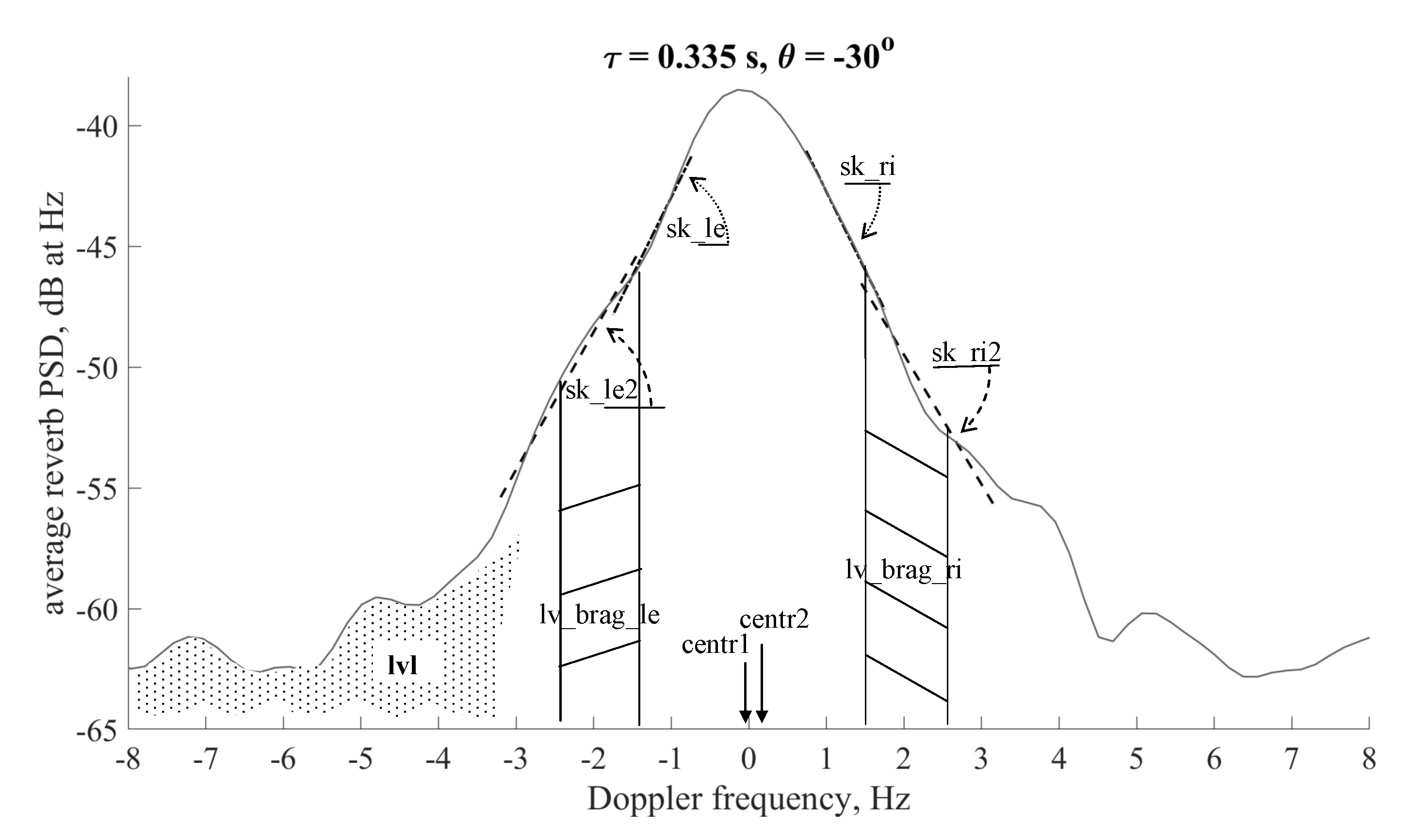
4.1. Signal Preprocessing and Features Extraction

We rely on so-called pulse-Doppler signal processing. It means that the scattering intensity is measured using a proper band pass filter. Since the direct signal is intended to be narrow-band enough, it can be suppressed by selecting the Doppler frequencies of the interest. Scattering intensity is measured during the time interval with proper delay, which is relative to a pulse transmission moment. In practice, such processing is done via short window Fourier transform and the spectrogram.

We start with the complex envelope with a sampling rate of 50 Hz at 4 carrier frequencies. Thirteen channels were used to form the directivity pattern in the directions from −90${}^{\circ }$ to +90${}^{\circ }$ with a step of 30${}^{\circ }$ (The total number of channels was 32, but it was reduced due to technical problems.) Then, the spectrogram of the complex signal for each direction was calculated. The length of the window was 64 samples, and the overlapping was 75%. The moment of the beginning of each pulse was determined for time synchronization in order to cut and save each pulse. Thus, at each carrier frequency, the dataset is the power spectral density of the received audio signal $PSD(\tau ,\Delta f,n,\theta )$, where $\tau$ is the delay, $\Delta f$ is the frequency shift relative to the carrier frequency, n is the pulse sequential number, and $\theta$ is the phasing angle.

From Section 2, we have gained some ideas about the possible dependence of the shape of the backscattering spectrum on the state of the sea. The original dataset is transformed to obtain input data whose dimension is comparable to the number of measurements.

First, we average over about twenty pulses ${\langle PSD(\tau ,\Delta f,n,\theta )\rangle }_n$ , which corresponds to a time step of 30 min. Bad pulses, whose echos are distorted by noise, are excluded from averaging. For example, in the daytime, the broadband noise from motor boats, ships, and the operations on the platform is especially noticeable compared to the signal. Such noise records are excluded based on the histogram criterion: the pulse is bad if the spectrogram has more than 5% of points exceeding the threshold value in the certain area on $\Delta f-\tau$ plane. An example of the averaged reverberation spectrogram is shown in Figure 4. The red zone, located on the plot from −3.3 to 0 over the time axis, is the time period when the receiver is saturated by the initial signal. When we speak about such saturation, initial pulse length is expanded by the intervals, when a Fourier window overlaps the initial pulse. We analyze the spectrogram in the area of positive time values and until the signal-to-noise ratio allows us to do this.

Second, the dependence on the Doppler frequency $\Delta f$ is recalculated into spectrum features. Scattering on bubbles leads to a triangular-like shape of the spectrum, it is reasonable to describe it by a slope. Closer to the Bragg frequency, the slope may change due to the surface scattering. Thus, we calculate the skew of the spectrum in the 2 frequency ranges.

The total level of backscattered signal and the signal level across the Bragg frequency can also be informative parameters. To estimate the central Doppler frequency, we introduce two frequency averages: the weighted average and the median average frequency. The last one should better take into account inequality or possible bumps on the tail of the distribution. The dependence on the angle $\theta$ and the time delay $\tau$ is preserved. Nine features for seven directions and eight time delays give us a total of 504 extracted features.

Figure 5 explains how the features are computed. Actually, it shows an average by pulse PSD of reverberation in logarithmic scale taken from direction $-{30}^{\circ }$ with a time delay of 0.35 s after pulse. This plot is a section of a pattern like Figure 4.

We have accepted the following notation. Each feature is labeled as a literal string name $\theta$$\tau$. $\theta$ is given in degrees, $\tau$ in seconds from the end of the initial pulse. Name is one of the following:

(1,2) sk_le & sk_ri [dB/Hz]—spectrum skew ( the coefficient for the approximation of the polynomial of the first degree by the least squares method in Doppler frequency diapason [−1.75; −0.75] or [0.75; 1.75]) for negative and positive Doppler frequencies, respectively.

(3,4) sk_le2 & sk_ri2 [dB/Hz]—the same features as (1,2) but calculated in a more distant frequency range ( [1.5; 3.2] for 2 kHz carrier frequency)

(5,6) centr1 & centr2 [Hz]—weighted average and the median average frequencies, respectively.

(7,8) lv_brag _le & lv _brag _ri [dB]—signal levels in the range of 1 Hz around the Bragg frequency ( −2 ± 0.5 Hz & 2 ± 0.5 Hz, respectively). It is worth mentioning that the illustration in the form of an area under the logarithmic PSD is inaccurate; in fact, the sum is calculated from PSD on a linear scale.

(9) lvl [dB]—total level of backscattered signal.

However, the horizontal line array, which is the available instrument, leads to the ambiguity in bearing estimation. Namely, the beamforming algorithm output is a function of the acoustic wave number projection on the line of the array. This leads to the presence of two equal lobes in the 0..360 degrees range. One can get only the sum of signals from these two directions. The directions, labeled as $-{90}^{\circ }$ and ${90}^{\circ }$, are free from such errors since they go along the line of the array, However, antenna concentration is the worst in those directions.

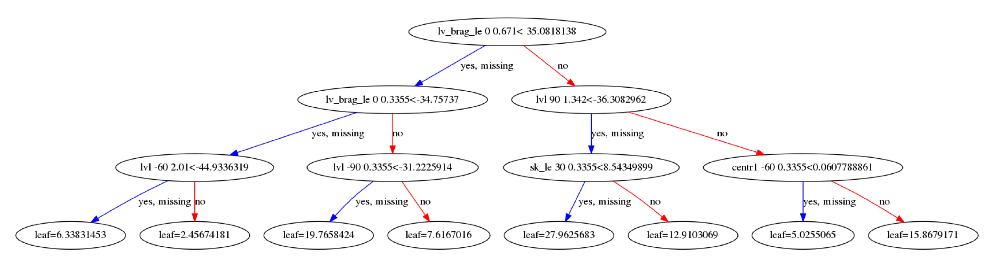
4.2. Regression Model

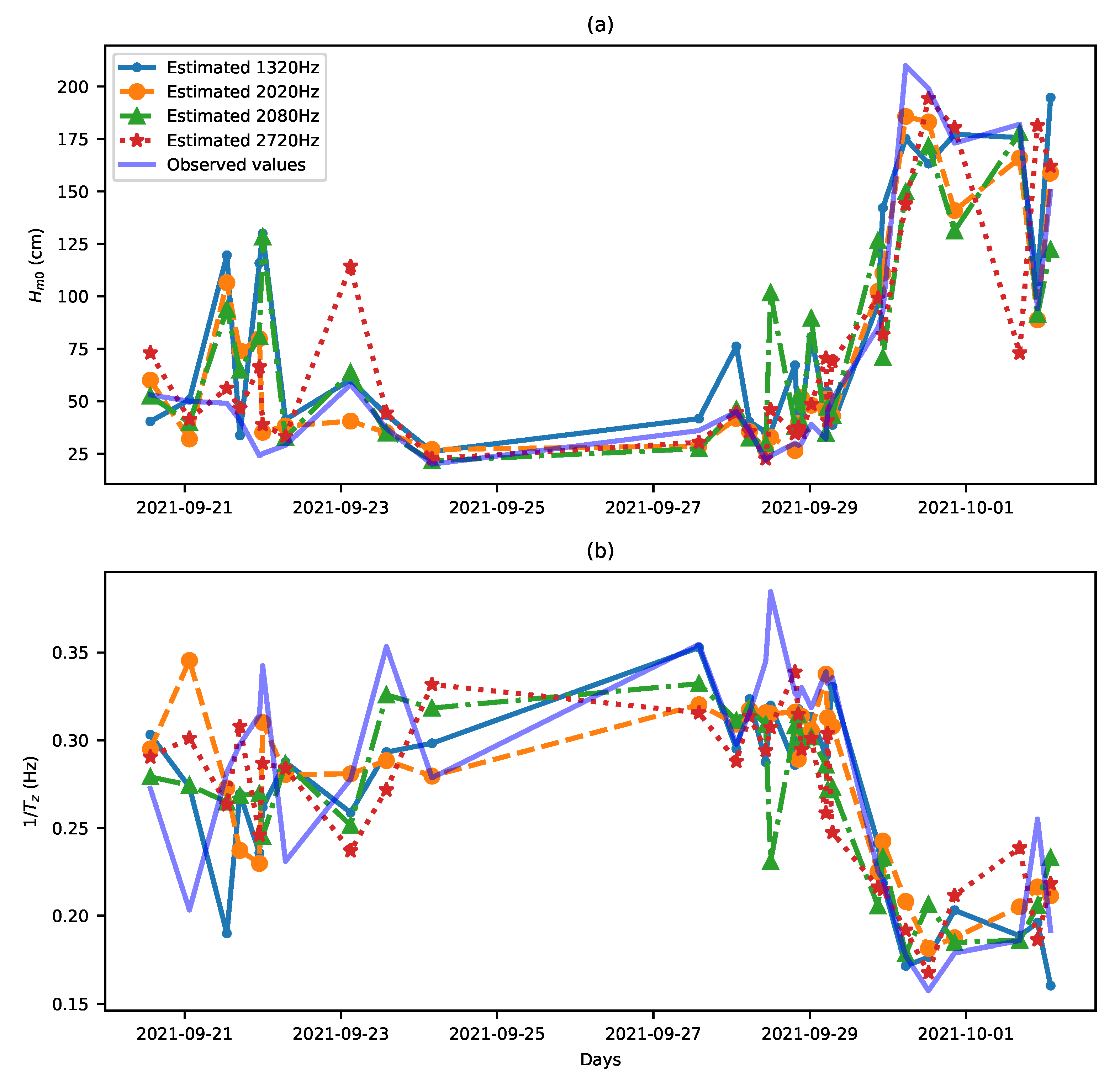
The goal of regression analysis is to establish a relationship between a dependent variable (outcome) and one or more independent variables (predictors, features). The regression model determines a functional space, where the particular function is chosen by establishing a set of parameters. A linear regression is an example of the simplest case, but not the best one. In a more complex case, the function space can be nonlinear. One possible way to build a nonlinear function is to build a regression tree. Many algorithms to build a regression tree that fit a function on observed data were developed. Most notable algorithms are ID3 [40], C4.5 [41], CART [42], and multivariate adaptive regression spline (MARS) [43]. To use an ensemble of regression trees is a natural idea to increase accuracy. Extreme Gradient Boosting (XGBoost) [35] is one of the leading algorithms that is based on this idea. It has been used successfully for the last several decades in different areas, including physical experiments [44]. In the present paper, we propose a method based on such model. We used a well known open source library (https://github.com/dmlc/xgboost; accessed on 22 May 2022) as an implementation of XGBoost algorithm. The linear regression was used as a baseline, and it was implemented as a polynomial fitting.

Figure 6 presents an example of a regression tree, built by the XGBoost algorithm. The input data (namely the values of extracted features, listed above) are compared with some threshold values in multiple yes/no tests. The model should be trained first. At this stage, both input (acoustic features) and output (surface waves state) are given to the software. It selects which feature to compare in each cell and adjusts the threshold values in order to minimize a loss function (error function). Here, as a loss function, we took the root mean square error (RMSE):

$$RMSE=\sqrt{\frac{1}{n}\sum _{i=1}^n{(Y_i-\widehat{Y_i})}^2}$$

(9)

where $Y_i$ is observed value, while $\widehat{Y_i}$ is estimated value. The tree, plotted on Figure 6, is a real example, produced by the software for our data. After training is done, the model is ready to make estimations. Thus, we feed the acoustic features as an input, and get the surface waves parameters as an output, which we compare with the real observed values.

5. Results

5.1. Correlation Analysis

Prior to exploiting machine learning methods, we start from direct comparison of environmental parameters and acoustic signal features. Figure 7 shows various features as functions of the significant wave height $H_{m0}$. Each marker on this and following plots correspond to data, obtained in the 30-min period during the whole experiment. The acoustic features, retrieved at the smallest possible time delay, are chosen here to analyze backscattering from the area that is close to the transducer and receiver, due to the instrument for direct measurement of $H_{m0}$ is located there. Recall that negative angles are when a scattering signal is received for the open sea, and, at positive angles, scattering takes place between the platform and the shore.

As it has been said in Section 2, spectral bandwidth of the scattered signal is expected to increase with the increase of the wave height. However, due to the bottom scattering, which dominates on the zero Doppler frequency, a classical −3 dB bandwidth appeared to be not a very reliable parameter for the present dataset. Such bandwidth is not treated as a feature at all, and the other feature (Figure 7a), describing how fast the spectral curve decays in 0.75–1.75 Hz span, is used instead of that one. Its value is negative and approaches zero, when the spectrum becomes more gently sloping. Scattering level at the Bragg frequency is also examined (see Figure 7b) since an increase in bandwidth should result in an increase in side lobes.

One may conclude that the spectral skew and the Bragg level are definitely correlated with the significant wave height. A linear or square parametrization is found for these features, using logarithmic scales on both axes. The plotted parametrization is found, using the dataset, obtained at mild sea states (namely the dataset plotted on the corresponding right panels: Figure 7d–f). Extrapolation of these data points match the other part of the dataset with over-meter wave heights. In addition, 90% of points fall into the plotted confidence interval on the right column of plots, and 80% on the left column of plots.

Exclusion of points with a relatively large shift of the Doppler centroid helped to reduce the dispersion. The reason for that is the fact that the presence current results in a change of all features. The most probable effect is that the whole triangle-shaped spectrum is moved. Surprisingly, no correlation is found for total backscattering level (see Figure 7c), despite many papers reports that this feature depends on the wind speed. Finally, examples of backscattering spectra, corresponding to some points on the above figures, are showed in Figure 8. Processing of these spectra resulted in extreme or vice versa mean values of such features as Doppler centroid and spectral skew.

From this section, one may conclude that the backscattering spectrum turns out to be determined by a complicated mixture of physical effects. Attempt to find a direct link between single input and single output parameters, matched with the respect to the theory, demonstrated some correlation, but the precision is not enough for practical usage. Proper inversion (i.e., computing surface waves parameters from spectral features) can be done using the machine learning methods, and this is going to be shown in the following subsection.

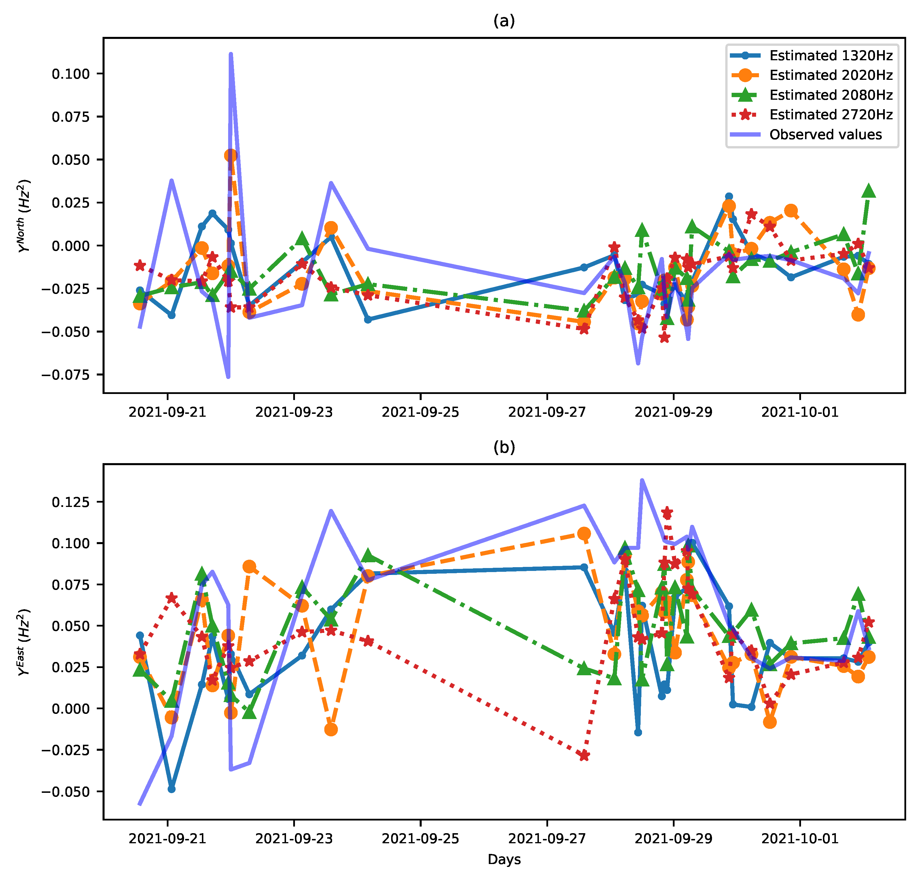
5.2. Evaluation of Regression Models

Accounting for several features together was achieved by feeding their values into the XGBoost algorithm. The model was built, trained, and tested, as it was described in Section 4.2. Common practice for such kind of testing is to split all experimental data into two non-overlapping parts that are going to be used for training and for testing separately. Here, the data were randomly split to train and test datasets by portion 10:1.

Figure 9 and Figure 10 show the results of testing stage. Various parameters of surface waves are plotted as they were estimated by the model. Recall that the model is XGBoost preceded by the feature extractor that processed the acoustic signal at available frequencies from 1320 to 2720 Hz (single frequency was tested at one time). The true values are plotted in Figure 9 and Figure 10 as well. Only points that belong to the testing dataset are plotted. There are gaps between them on the timeline, where the training data were obtained.

To evaluate the performance of the regression modes, we used cross validation with 10 folds. Thus, the data were split by five no-overlapping parts. Each part was used as a test set for model evaluation, while four remaining parts were used as a training test to fit the model. For a particular model, we calculate the mean and standard deviation over five RMSE values for each fold. RMSE values are presented in

Table 1. RMSE values for XGBoost regression equipped with 30 trees with max depth of 3 on cross validation with 5 fold.

Frequency	North Projection	East Projection	Squared Wave Frequency	Wave Height
(Hz)	${\mathit{Y}}^{\mathbf{North}}$ (Hz${}^2$)	${\mathit{Y}}^{\mathbf{East}}$ (Hz${}^2$)	${\mathit{Y}}^{\mathit{F}2}$ (Hz${}^2$)	${\mathit{H}}_{\mathit{m}0}$ (cm)
1320	0.0303	0.0595	0.0282	47
2020	0.0297	0.0612	0.0258	39
2080	0.0300	0.0585	0.0256	42
2720	0.0316	0.0580	0.0238	35

.

In

Table 2. RMSPE (Root Mean Square Percentage Error) values for XGBoost regression model equipped with 30 trees with max depth of 3 on the test set.

Frequency	North Projection	East Projection	Squared Wave Frequency	Wave Height
(HZ)	${\mathit{Y}}^{\mathbf{North}}$ (%)	${\mathit{Y}}^{\mathbf{East}}$ (%)	${\mathit{Y}}^{\mathit{F}2}$ (%)	${\mathit{H}}_{\mathit{m}0}$ (%)
1320	288.3	78.0	32.6	116
2020	332.6	76.1	36.8	45.7
2080	233.4	63.9	36.9	103
2720	118.0	111.6	37.4	57.3

, we present the values RMSPE (Root Mean Square Percentage Error) that were calculated according to (10) on the test set:

$$RMSPE=\sqrt{\frac{1}{n}{\sum }_{i=1}^n{\left(\frac{Y_i-\widehat{Y_i}}{Y_i}\right)}^2}$$

(10)

The most precise (see Table 2) prediction was done for $Y^{F2}$, namely 33% error was achieved, which resulted in 16% error of determining the peak frequency. Next comes significant wave height, estimated with a 46% error. The worst result was for $Y^{\mathrm{North}}$: the error is the same order of magnitude as the parameter value by itself. This performance was obtained for the parameters: tree max depth of 4, number of estimators of 24, and learning rate of 0.1. (Learning rate influences to what extent newly acquired information overrides old information.)

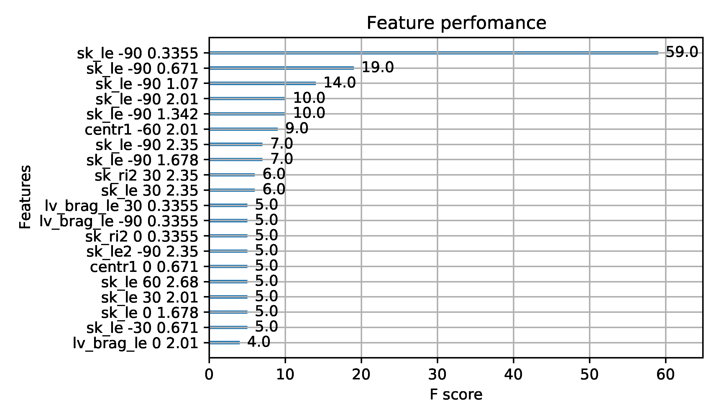
5.3. Parameters Tuning

By using grid search with 10 folds for cross validation, we examined XGBoost regression model with the following parameters:

• Number of estimators $=1,2,\dots ,299$;
• Max depth of decision trees $=1,2,\dots ,10$;
• Learning rate $=0.1,0.05,0.01$;
• Step size shrinkage $\eta$$=0.3$.

Table 3. The results of parameter tuning of the XGBoost regression model for predicting $H_{m0}$, done by grid search.

	Mean RMSE	std of RMSE	Max_Depth	n_Estimators	Learning_Rate
1320 Hz	40.4	37.3	3	193	0.10
2020 Hz	32.1	30.9	3	154	0.05
2080 Hz	38.6	32.3	3	276	0.05
2720 Hz	34.3	38.5	2	207	0.05

presents results of the parameters tuning. The table shows that the model is stable with respect to its adjustable parameters.

6. Discussion

The described experiment showed a principal possibility to estimate the parameters of energy-carrying surface waves using underwater sound of the mid-frequency band. We recognize that we have provided comparison of local and remote measurements and that might be not completely correct.

The most remarkable fact is that the algorithm was not aware of existing physical models at all; nevertheless, according to Figure 11, it had selected features, related to our prior theoretical expectations. For example, spectral skew appeared to be a very useful feature for machine learning, as well as having shown good results during the correlation analysis (Figure 7). Moreover, features, corresponding to signals, coming from open sea and small delays were prioritized to estimate surface state in the center of coordinates. On the other hand, during the first attempt to process the data, we missed the time synchronization and the model did not produce any meaningful result until we fixed that. Thus, we did not overestimate the possibilities of the machine learning. It was the successful choice of features, based on the correct understanding of physical processes that made it possible to train the model to make the correct prediction with such a small training sample.

The measurement technique can be significantly improved. First, the design of the hydrophone array may be improved to avoid left-right ambiguity. For example, one can use a circular array or an array of vector sensors. Second, several transmitters and receivers are required for better measurement of both projections of the current speed in the same cell. As mentioned, the wavenumber projections of surface waves were estimated with low precision. Co-location of this measurement system with a coastal acoustic tomography system [17] may be suggested. Third, special frequency modulated signals may reduce the size of the measurement cell; however, proper correspondence between Doppler scattering strength in case of tonal and frequency-modulated signals should be studied to do so [33]. Careful filtering of bottom scattering should be provided as well.

After all, the underlying physics is still not completely clear. We started from two concurring models: surface Bragg scattering of sound and bubble scattering. We still cannot prove that one of them is dominant. If one has accepted the bubble scattering model, then one should expect the increase of scattering strength in case of strong wind and large wave heights due to an increasing number of bubbles. However, no significant increase of scattering strength was detected during all stages of the experiment (To be more precise, a 4 dB increase was found at some specific condition of strong wind with short fetch, but not enough statistical information was collected to make any conclusion from that event).

One more issue with our data is that a spectrum, received from one pulse in one resolution cell, appeared to be too stochastic, i.e., spectra varied greatly from pulse to pulse. Smooth curves were obtained only after averaging up to 20 pulses. However, scattering took place on an area around a square kilometer, where the sound must have interacted with many scatterers, so we expected the result should have been averaged over an ensemble.

The proposed technique is in some aspects analogous to satellite-based synthetic apertures radar applications [45], where remote measurement results are affected by a group of factors and the data undergo model-based calibration procedures too. By now, the precision, achieved in the proposed acoustical method, is nominally lower than can be reached by the existing methods. The proposed technique of mid-frequency echosounding in horizontal plane is going to be useful due to it having other conditions of applicability. Marine radars [6,7,8,9] stick to a platform or are limited by weather conditions, when ships can operate. Bottom-mounted self-contained acoustic devices can carry out measurements when above-the-water operations are stopped due to heavy storms or the presence of drifting ice. This is true for other kinds of acoustic tools [10,11,12] too, but high frequency echosounders provide less propagation range than the proposed instuments.

The important advantage of the presented experimental scheme is the possibility of exploitation of the Bragg resonance to directly measure components of surface waves spectrum with K = 10..20 rad/m. This fact is not fully revealed in this paper because, up to now, we have mainly focused on the dominant wave parameters retrieval. However, the mentioned wavenumbers range is quite important too, and it seems not to be easily accessible by ship-mounted radars. As for current experimental results, the “sk_le” and “sk_ri” features helped us to eliminate experimental spectra with gentle sloping of the central peak. In the remaining cases with sharp central peaks, we do observe moderate enhancement on Bragg frequencies; for example, see ‘−18 dB/Hz’ and ‘−24 dB/Hz’ curves of Figure 8b. More thorough study on this topic is going to be carried out further.

7. Conclusions

The described experiment showed principal possibility to estimate the parameters of energy-carrying surface waves using underwater sounds of the mid-frequency band. The machine learning method, called XGBoost, was exploited, and physical interpretation helped to reduce the size of the input data by selecting proper features on the first stage of signal processing. Training (or calibration) of a model was required prior to its usage for estimations and, at this stage, the local data were used. The testing was done so that the parameters of interest were estimated in the "center of coordinates", while the algorithm was processing acoustic reverberation spectra, received from remote points, located in about a kilometer range from that point.

The developed signal processing algorithm can be applied to estimating surface state in remote points. However, one more experimental study with a modified scheme might be helpful to directly check the remote sensing function. The way the regression model behaves towards various input data along with the correlation analysis results is a motive for further development.

References

1. Kuznetsova, A.; Baydakov, G.; Papko, V.; Kandaurov, A.; Vdovin, M.; Sergeev, D.; Troitskaya, Y. Adjusting of wind input source term in WAVEWATCH III model for the middle-sized water body on the basis of the field experiment. Adv. Meteorol. 2016, 2016, 1–13. [Google Scholar] [CrossRef] [Green Version]
2. Wei, Z.; Davison, A. A convolutional neural network based model to predict nearshore waves and hydrodynamics. Coast. Eng. 2022, 171, 104044. [Google Scholar] [CrossRef]
3. Young, I.R.; Rosenthal, W.; Ziemer, F. A three-dimensional analysis of marine radar images for the determination of ocean wave directionality and surface currents. J. Geophys. Res. Ocean. 1985, 90, 1049–1059. [Google Scholar] [CrossRef] [Green Version]
4. Dankert, H.; Horstmann, J.; Rosenthal, W. Wind-and wave-field measurements using marine X-band radar-image sequences. IEEE J. Ocean. Eng. 2005, 30, 534–542. [Google Scholar] [CrossRef]
5. Rosenberg, A.; Ostrovskiy, I.; Zel’dis, V.; Leiykin, I.; Ruskevich, V.G. Determination of the energy-carrying part of the sea wave spectrum by the phase characteristics of the radio signal scattered by the sea. Izv. Akad. Nauk SSSR Fiz. Atmosfery i Okeana 1973, 9, 1323–1326. (In Russian) [Google Scholar]
6. Lyzenga, D.; Nwogu, O.; Trizna, D.; Hathaway, K. Ocean wave field measurements using X-band Doppler radars at low grazing angles. In Proceedings of the 2010 IEEE International Geoscience and Remote Sensing Symposium, Honolulu, HI, USA, 25–30 July 2010; pp. 4725–4728. [Google Scholar] [CrossRef]
7. Carrasco, R.; Horstmann, J.; Seemann, J. Significant wave height measured by coherent X-band radar. IEEE Trans. Geosci. Remote. Sens. 2017, 55, 5355–5365. [Google Scholar] [CrossRef]
8. Ermoshkin, A.; Kapustin, I. Estimation of the wind-driven wave spectrum using a high spatial resolution coherent radar. Russ. J. Earth Sci. 2019, 19, 1. [Google Scholar] [CrossRef] [Green Version]
9. Ermoshkin, A.; Kapustin, I.; Molkov, A.; Bogatov, N. Determination of the sea surface current by a Doppler X-band radar. Fundam. Prikl. Gidrofiz. 2020, 13, 93–103. (In Russian) [Google Scholar] [CrossRef]
10. Adibzade, M.; Shafieefar, M.; Akbari, H.; Panahi, R. Multi-peaked directional wave spectra based on extensive field measurement data in the Gulf of Oman. Ocean. Eng. 2021, 230, 109057. [Google Scholar] [CrossRef]
11. Titchenko, Y.; Karaev, V.; Ryabkova, M.; Meshkov, E. Measurements of the sea surface parameters using a new modification of underwater sonar on a marine platform in the Black Sea. In Proceedings of the OCEANS 2019-Marseille, Marseille, France, 17–20 June 2019; pp. 1–7. [Google Scholar] [CrossRef]
12. Titchenko, Y.; Karaev, V.; Ryabkova, M.; Kuznetsova, A.; Meshkov, E. Peculiarities of the Acoustic Pulse Formation Reflected by the Water Surface: A Numerical Experiments and the Results of Long-term Measurements Using the “Kalmar” Sonar. In Proceedings of the OCEANS 2019-Marseille, Marseille, France, 17–20 June 2019; pp. 1–7. [Google Scholar] [CrossRef]
13. Salin, M.; Potapov, O.; Salin, B.; Chashchin, A. Measuring the characteristics of backscattering of sound on a rough surface in the near-field zone of a phased array. Acoust. Phys. 2016, 62, 74–88. [Google Scholar] [CrossRef]
14. Badiey, M.; Eickmeier, J.; Song, A. Arrival-time fluctuations of coherent reflections from surface gravity water waves. J. Acoust. Soc. Am. 2014, 135, EL226–EL231. [Google Scholar] [CrossRef] [Green Version]
15. Richards, E.L.; Song, H.C.; Hodgkiss, W.S. Observations of scatter from surface reflectors with Doppler sensitive probe signals. JASA Express Lett. 2021, 1, 016001. [Google Scholar] [CrossRef]
16. Huang, C.F.; Li, Y.W.; Taniguchi, N. Mapping of ocean currents in shallow water using moving ship acoustic tomography. J. Acoust. Soc. Am. 2019, 145, 858–868. [Google Scholar] [CrossRef]
17. Kaneko, A.; Zhu, X.H.; Lin, J. Coastal Acoustic Tomography; Elsevier: Amsterdam, The Netherlands, 2020. [Google Scholar]
18. Chen, M.; Zhu, Z.N.; Zhang, C.; Zhu, X.H.; Zhang, Z.; Wang, M.; Zheng, H.; Zhang, X.; Chen, J.; He, Z.; et al. Mapping of tidal current and associated nonlinear currents in the Xiangshan Bay by coastal acoustic tomography. Ocean. Dyn. 2021, 71, 811–821. [Google Scholar] [CrossRef]
19. Goncharov, V.; Kuryanov, B.; Serebryany, A. Local acoustic tomography on shelf of the Black Sea. Hydroacoustics 2013, 16, 67–76. [Google Scholar]
20. Dahl, P.H.; Plant, W.J.; Nützel, B.; Schmidt, A.; Herwig, H.; Terray, E.A. Simultaneous acoustic and microwave backscattering from the sea surface. J. Acoust. Soc. Am. 1997, 101, 2583–2595. [Google Scholar] [CrossRef]
21. Salin, B.M.; Salin, M.B.; Spindel, R.C. Calculation of the reverberation spectrum for Doppler-based sonar. Acoust. Phys. 2012, 58, 220–227. [Google Scholar] [CrossRef]
22. Bjørnø, L. Chapter 5—Scattering of Sound. In Applied Underwater Acoustics; Neighbors, T.H., Bradley, D., Eds.; Elsevier: Amsterdam, The Netherlands, 2017; pp. 297–362. [Google Scholar] [CrossRef]
23. Dolin, L.S.; Kondratyeva, M.I. On the possibility of reconstructing an anisotropic wind wave spectrum by the method of double-position sonar. Radiophys. Quantum Electron. 1995, 38, 93–97. [Google Scholar] [CrossRef]
24. Hayek, C.S.; Schurman, I.W.; Sweeney, J.H.; Boyles, C.A. Azimuthal dependence of Bragg scattering from the ocean surface. J. Acoust. Soc. Am. 1999, 105, 2129–2141. [Google Scholar] [CrossRef]
25. Urick, R.J. Principles of Underwater Sound, 3rd ed.; McGraw Hill Higher Education: Maidenhead, UK, 1983. [Google Scholar]
26. Neighbors, T.; Bjørnø, L. Anomalous low frequency sea surface reverberation. Hydroacoustics 2001, 4, 181–192. [Google Scholar]
27. Thorpe, S.A. On the clouds of bubbles formed by breaking wind-waves in deep water, and their role in air-sea gas transfer. Philos. Trans. R. Soc. London. Ser. A Math. Phys. Sci. 1982, 304, 155–210. [Google Scholar]
28. Deane, G.B.; Stokes, M.D. Scale dependence of bubble creation mechanisms in breaking waves. Nature 2002, 418, 839–844. [Google Scholar] [CrossRef]
29. Akulichev, V.; Bulanov, V.; Bugaeva, L. Features of Sound Propagation in the Presence of Bubble Clouds in the Perturbed Surface Layer of the Ocean. Dokl. Earth Sci. 2019, 487, 1002–1005. [Google Scholar] [CrossRef]
30. Liu, R.; Li, Z. The Effects of Bubble Scattering on Sound Propagation in Shallow Water. J. Mar. Sci. Eng. 2021, 9, 1441. [Google Scholar] [CrossRef]
31. Salin, B.; Salin, M. Formation Mechanisms for the Spectral Characteristis of Low-Frequency Reverberations and Predictive Estimates. Acoust. Phys. 2018, 64, 196–204. [Google Scholar] [CrossRef]
32. Doisy, Y.; Deruaz, L.; van IJsselmuide, S.P.; Beerens, S.P.; Been, R. Reverberation suppression using wideband Doppler-sensitive pulses. IEEE J. Ocean. Eng. 2008, 33, 419–433. [Google Scholar] [CrossRef]
33. Rui, G.; Xiao-tong, W.; Zhi-ming, C. Comparison research on reverberation strength excited by PTFM and CW signals. In Proceedings of the 2016 IEEE 13th International Conference on Signal Processing (ICSP), Chengdu, China, 6–10 November 2016; pp. 1677–1681. [Google Scholar] [CrossRef]
34. Hartstra, I.; Colin, M.; Prior, M. Active sonar performance modelling for Doppler-sensitive pulses. Proc. Meet. Acoust. 2021, 44, 022001. [Google Scholar] [CrossRef]
35. Chen, T.; Guestrin, C. Xgboost: A scalable tree boosting system. In Proceedings of the 22nd ACM Sigkdd International Conference on Knowledge Discovery and Data Mining, San Francisco, CA, USA, 13–17 August 2016; pp. 785–794. [Google Scholar]
36. Ellis, D.D. A shallow-water normal-mode reverberation model. J. Acoust. Soc. Am. 1995, 97, 2804–2814. [Google Scholar] [CrossRef]
37. Kazak, M.; Koshel, K.; Petrov, P. Generalized Form of the Invariant Imbedding Method and Its Application to the Study of Back-Scattering in Shallow-Water Acoustics. J. Mar. Sci. Eng. 2021, 9, 1033. [Google Scholar] [CrossRef]
38. Lynch, J.; Newhall, A. Chapter 7—Shallow-Water Acoustics. In Applied Underwater Acoustics; Neighbors, T.H., Bradley, D., Eds.; Elsevier: Amsterdam, The Netherlands, 2017; pp. 403–467. [Google Scholar] [CrossRef]
39. Razumov, D.; Salin, M. Features of sound diffraction on surface roughness in the middle-frequency range. Fundam. Prikl. Gidrofiz. 2021, 14, 98–110, (In Russian, see doi:10.1109/DD52349.2021.9598681 for a close English version). [Google Scholar] [CrossRef]
40. Quinlan, J.R. Induction of decision trees. Mach. Learn. 1986, 1, 81–106. [Google Scholar] [CrossRef] [Green Version]
41. Quinlan, J.R. C4. 5: Programs for Machine Learning; Elsevier: Amsterdam, The Netherlands, 2014. [Google Scholar]
42. Breiman, L.; Friedman, J.H.; Olshen, R.A.; Stone, C.J. Classification and Regression Trees; Routledge: New York, NY, USA, 2017. [Google Scholar]
43. Friedman, J.H. Multivariate adaptive regression splines. Ann. Stat. 1991, 19, 1–67. [Google Scholar] [CrossRef]
44. Roe, B.P.; Yang, H.J.; Zhu, J.; Liu, Y.; Stancu, I.; McGregor, G. Boosted decision trees as an alternative to artificial neural networks for particle identification. Nucl. Instruments Methods Phys. Res. Sect. A Accel. Spectrometers Detect. Assoc. Equip. 2005, 543, 577–584. [Google Scholar] [CrossRef] [Green Version]
45. Mouche, A.A.; Collard, F.; Chapron, B.; Dagestad, K.F.; Guitton, G.; Johannessen, J.A.; Kerbaol, V.; Hansen, M.W. On the Use of Doppler Shift for Sea Surface Wind Retrieval From SAR. IEEE Trans. Geosci. Remote Sens. 2012, 50, 2901–2909. [Google Scholar] [CrossRef]
46. Razumov, D.; Ermoshkin, A.; Kosteev, D.; Ponomarenko, A.; Salin, M. Dataset for Surface waves prediction based on acoustic backscattering. 2022. Available online: https://zenodo.org/record/6530915 (accessed on 23 May 2022).
Figure 1. The numerical simulation results for backscattering spectra, when surface roughness is determined by the Pierson—Moskowitz spectra for sea states, which are labeled as (a) 1, (b) 2, (c) 3 and defined as follows: Peak frequencies: (a) 0.6, (b) 0.3 and (c) 0.2 Hz; the wind speeds: (a) 2.28, (b) 4.47 and (c) 6.84 m/s; P r = (a) 0.08, (b) 0.315 and (c) 0.72. The sound frequency is 1.5 kHz, incident and scattering grazing angles are 30 . Two models are exploited, where scattering is originated by rough surface and bubble clouds.
Jmse 10 00722 g001
Figure 2. Experimental scheme, top view, phasing and time strobing grid. An example of approximate scattering region delineated for a pulse length of 2 s.
Jmse 10 00722 g002
Figure 3. Experiment scheme in the vertical plane.
Jmse 10 00722 g003
Figure 4. An example of spectrogram of an acoustic signal.
Jmse 10 00722 g004
Figure 5. An example of the scattering spectrum with a sketch, explaining how it can be described by the selected set of features.
Jmse 10 00722 g005
Figure 6. An example of the decision tree of depth 4 for North projection formed by XGBoost for 2020 Hz frequency.
Jmse 10 00722 g006
Figure 7. Dependence between features and a significant wave height. A set of features is studied: (a) d o u b l e _ s k e w = s k _ r i s k _ l e , (b) l v l _ b r a g _ r i and (c) lvl that stands for a total level; (df) are scaled versions of (ac). Red filled dots are the data without a significant shift of Doppler centroid ( | c e n t r 1 | < 0.075 Hz) and stars represent the rest of the dataset. Dashed lines represent confidence intervals around a fitting line or curve. Right panels are scaled versions of left panels.
Jmse 10 00722 g007
Figure 8. Examples of the backscattering spectra, obtained in the experiment (Pay attention to the feature values, printed in the legend). Vertical dash lines point the Bragg frequencies for a reference.
Jmse 10 00722 g008
Figure 9. Comparison of 4 XGBoost regression models equipped by 20 decision trees of the max depth 10 utilizing features for different frequencies to estimate the projections of the effective wavenumber, namely: (a) the North projection and (b) the East projection.
Jmse 10 00722 g009
Figure 10. Comparison of 4 XGBoost regression models equipped by 20 decision trees of the max depth 10 utilizing features for different frequencies to estimate the values of (a) the significant wave height and (b) the peak wave frequency.
Jmse 10 00722 g010
Figure 11. Twenty most important features reported by the XGBoost algorithm. Frequency = 2720 Hz, number of estimators = 20. The importance means how many times the feature was used in the decision trees to split the data.
Jmse 10 00722 g011