
Impacts of Discretization and Numerical Propagation on the Ability to Follow Challenging Square Wave Commands


1
Sibley School of Mechanical and Aerospace Engineering, Cornell University, Ithaca, NY 14853, USA
2
Naval Information Warfare Training Command, U.S. Army Presidio, Monterey, CA 93944, USA
3
Department of Mechanical and Aerospace Engineering, Naval Postgraduate School, Monterey, CA 93943, USA
*
Author to whom correspondence should be addressed.
J. Mar. Sci. Eng. 2022, 10(3), 419; https://doi.org/10.3390/jmse10030419
Submission received: 26 January 2022
/
Revised: 1 March 2022
/
Accepted: 7 March 2022
/
Published: 13 March 2022
(This article belongs to the Special Issue Control, Guidance, Coordination, and Localization of Autonomous Marine Vehicles)
Abstract
:This study determines the threshold for the computational rate of actuator motor controllers for unmanned underwater vehicles necessary to accurately follow discontinuous square wave commands. Motors must track challenging square-wave inputs, and identification of key computational rates permit application of deterministic artificial intelligence (D.A.I.) to achieve tracking to a machine-precision degree of accuracy in direct comparison to other state-of-art approaches. All modeling approaches are validated in MATLAB simulations where the motor process is discretized at varying step-sizes (inversely proportional to computational rate). At a large step-size (fast computational rate), discrete D.A.I. shows a mean error more than three times larger than that of a ubiquitous model-following approach. Yet, at a smaller step size (slower computational rate), the mean error decreases by a factor of 10, only three percent larger than that of continuous D.A.I. Hence, the performance of discrete D.A.I. is critically affected by the sampling period for discretization of the system equations and computational rate. Discrete D.A.I. should be avoided when small step-size discretization is unavailable. In fact, continuous D.A.I. has surpassed all modeling approaches, which makes it the safest and most viable solution to future commercial applications in unmanned underwater vehicles.
1. Introduction
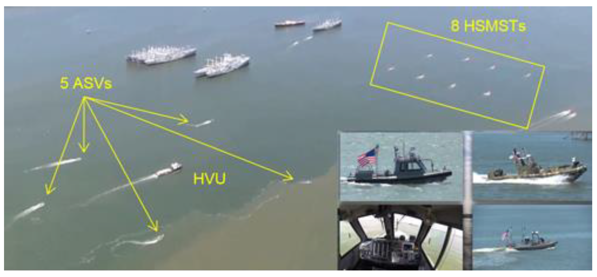
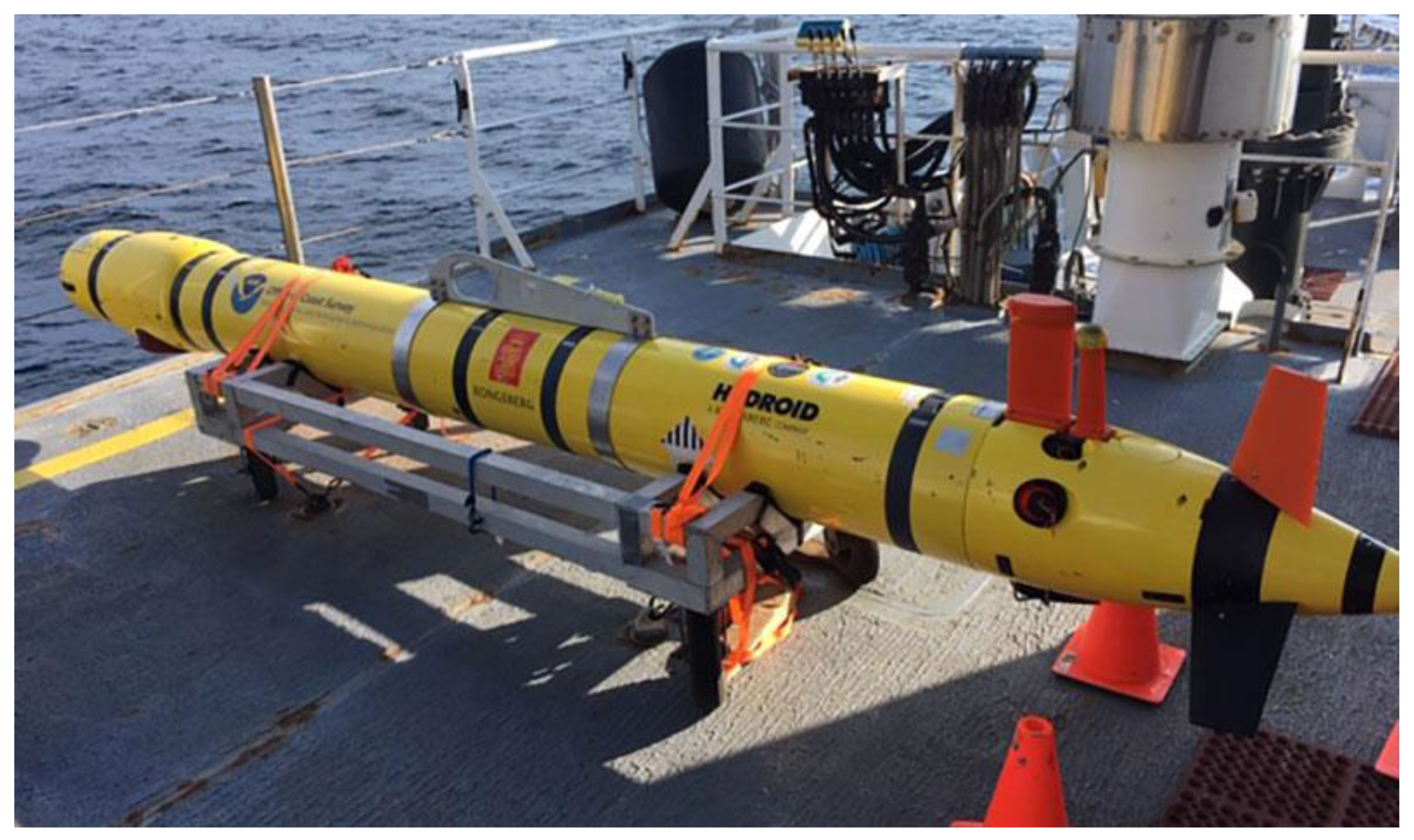
The United States Navy has that recognized unmanned vehicles are a key part of future naval capabilities [1], as depicted in Figure 1. The development of adaptive and learning systems has greatly expanded the possibility of unmanned vehicles, allowing human control in distant operations that are otherwise impossible. The automation of DC motor control has thus earned its latest highlight as a resurgent, promising field of research. Deterministic artificial intelligence (D.A.I.) utilizes self-awareness assertion in the feedforward process dynamics, where the feedback signal is formulated by 2-norm optimal least squares (learning) or by proportional derivative feedback (adaption). This manuscript serves both as a sequel to the analysis of discrete D.A.I. (described in the following literature review), and the publication is written advocating for commercial application of D.A.I. to unmanned vehicles as depicted in Figure 2. The main text includes an in-depth comparison to a chosen state-of-the art benchmark approach mainly focusing on their disparate trajectory tracking ability.
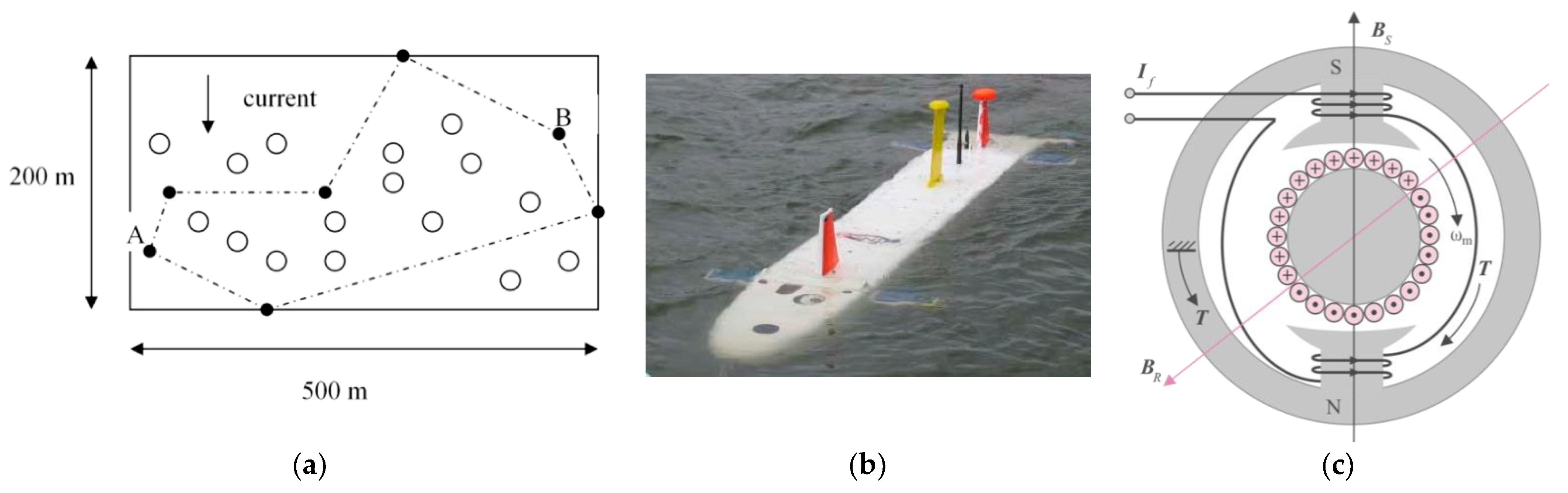
Reference [2] describes a tightly integrated instantiation of an autonomous agent called CARACaS (Control Architecture for Robotic Agent Command and Sensing) developed at JPL (Jet Propulsion Laboratory, Pasadena, USA) that was designed to address many of the issues for survivable ASV/AUV control and to provide adaptive mission capabilities (see Figure 1). Missions naturally suited for utilization include traverse, mapping, and potentially neutralizing mine fields [5,6], as displayed in Figure 3 from the study in reference [7] for the Phoenix vehicle in Figure 3b.
The development of adaptive and learning systems has a long, distinguished lineage in the literature [8,9,10,11,12,13,14,15,16,17,18,19,20,21,22,23,24,25,26,27,28,29,30,31,32,33,34,35] with many optional techniques available to choose from. The trendsetting work of Isidori and Byrnes [36] on the control of exogenous signals revealed the close tie between the nonlinear regulator equations and the output regulation of a nonlinear system. The momentum continued, and the nonlinear output regulation has been further explored by numerous authors including Cheng, Tarn, and Spurgeon [37], Khalil [38], and Wang and Huang [39] across autonomous and nonautonomous systems. The lineage emphasized in this manuscript stems from a heritage in vehicle guidance and control techniques [8,9,10,11,12,13,14,15] extended to apply to motor controllers [17,18,19,20,21,22,23,24,25,26,27,28,29,30,31,32,33,34,35] that generate vehicle motion. Vehicle maneuvering is controlled by the actuator fins displayed in Figure 3b generating navigation as displayed in Figure 3a. Actuation is accomplished by sending control signals to motors (Figure 3c) that rotate the fins.
This manuscript proposes a preferred instantiation of adaptive and learning systems [26,27] by evaluating the efficacy of motor control techniques based on iterated computational rates and system discretization. The materials and methods in Section 2 first describe model discretization and then introduces the two compared: one adaptive and one learning each with interconnected lineage of research in the literature.
1.1. Learning Teachniques
The learning techniques examined in this manuscript stem from heritage in Slotine and Li’s nonlinear adaptive methods developed originally for robotics [8] and spacecraft [9,10,11], while the method has been similarly applied to ocean vehicles [14,15]. The method was initially expressed in the non-rotating inertial reference frame [8,9] and resulted in cumbersome numerical burdens, therefore Fossen re-parameterized the method into the coordinates of the body reference frame [10], while [11] illustrated separate tunability of feedforward and feedback elements. The feedforward elements substantiated what eventually became known as self-awareness statements [12] of deterministic artificial intelligence [13].
Fossen also prolifically published application to ocean vehicles [14] including the most recent text [15] which includes contains trajectory tracking control via pole placement PID, LQR, feedback linearization, nonlinear backstepping, sliding mode control, which might now be deemed commonly accepted approaches. Reference [7] illustrates the efficacy of such approaches to guide autonomous underwater vehicles through simulated minefields illustrated in Figure 3a,b. The feedforward elements were used to develop deterministic artificial intelligence through maturation as applied in so-called physics-based methods championed by Lorenz [16] and his students [11,17,18,19,20,21,22,23,24] for many years, which also extended the method from vehicles to actuator control circuits where representative results following challenging discontinuous commands are depicted in Figure 4. Zhang et al. [17] illustrated fault-tolerance, while Apoorva et al. [18] revealed loss reduction and Flieh et al. demonstrated loss minimization [19] and dead-beat control [20] in addition to self-sensing [21], the precursor to using the physics-based dynamics for virtual sensing [22] following the illustration of optimality in [23] and self-sensing [24] specifically applied to DC motors.
Despite stochastic learning methods still holding some interest [25] applied to motor control, this manuscript continues the investigation of deterministic learning approaches [26] following Shah’s recommendations [27]. Specifically, [26] illustrated a marked improvement in tracking performance, while Shah’s attempt in [27] to duplicate the results revealed a strong correlation to performance improvement and system discretization and speed of computation. One novelty presented here is analysis of Shah’s identified correlated factors.
1.2. Adaptive Techniques as Benchmarks for Comparison
Many alternative approaches are available as benchmarks for comparison. A short survey of alternative methods is presented in [30] presenting multiple model adaptive control (MMAC) techniques available for the control of a DC motor under load changes. Direct torque control is an option based on discontinuities in rapid modulating commands. [31] Speed control is presented using a model-reference adaptive control in [32] offering the possibility to compensate the torque ripples and load torque. Akin to the optimization approach applied to vehicles (second order systems) [22], extremum-seeking adaptive control of first-order systems was proposed in [33,34].
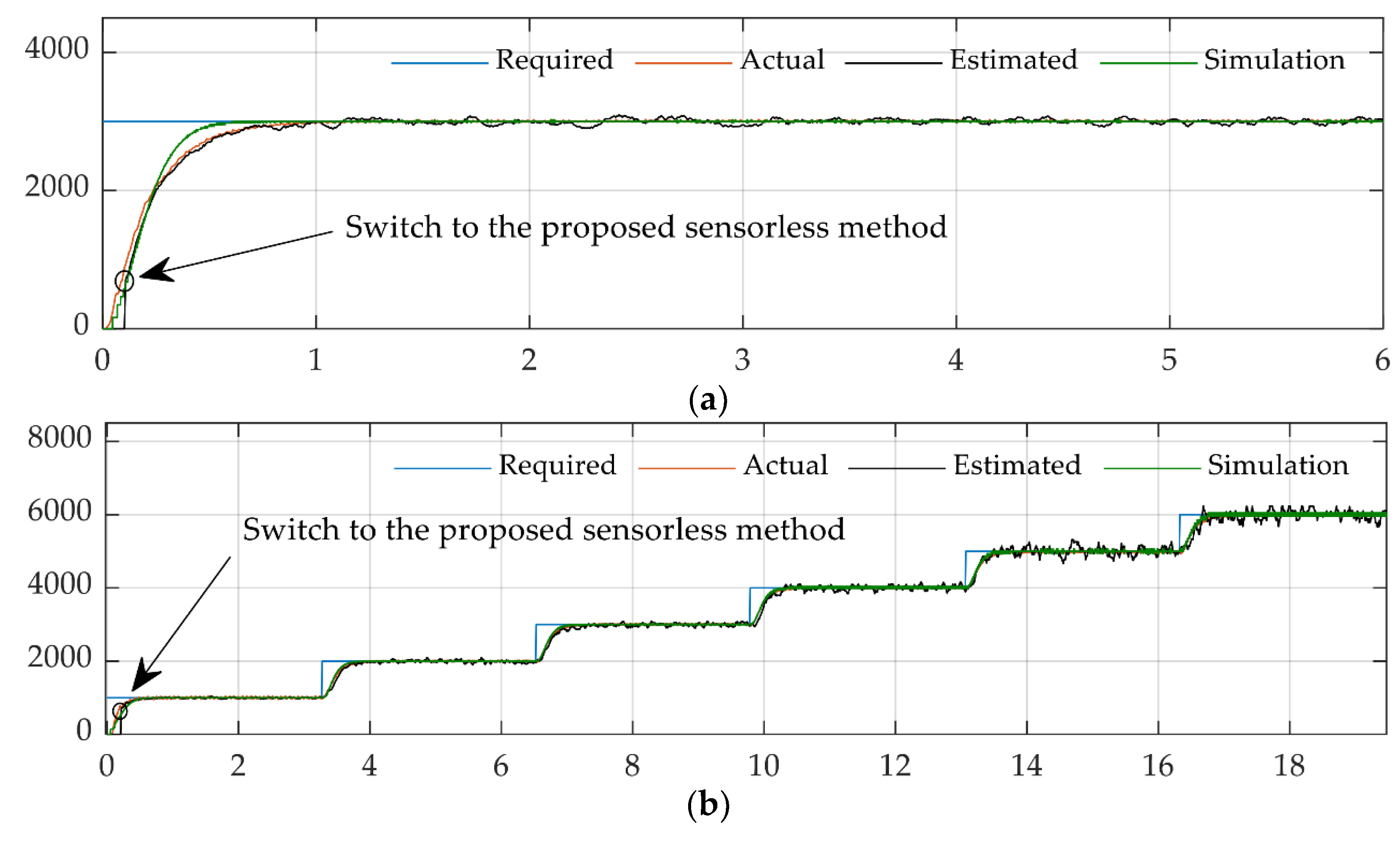
Alternative approaches are generally tested with step and/or square wave inputs. The ability to track step functions or square wave sequences of step functions is a challenging requirement for DC motor control. Square wave command is chosen because the tracking ability of a nonlinear adaptive method can easily be discerned by the magnitude of overshoot and undershoot at the discontinuities in the square wave. Figure 4 validates the challenge by illustrating a just-published novel sensor-less methods struggling to follow step and square wave commands, respectively. Figure 5 displays the results of model reference adaptive control and robust adaptive control in Figure 5a and self-tuning regulators in Figure 5b. These methods display disparate natures illustrating the difficulties.
The chosen comparative benchmark adaptive technique is the model-following self-tuning regulator [28] in keeping with the prequel research by Shah [27] who sought to duplicate the results in [26], which seemingly exactly followed a challenging square wave (with non-rounded discontinuous points) after an initial startup transient.
Following the publication of [26], Shah et al. revealed performance limitations in [27] indicating computational rate is the driving influence when the system is discretized. This manuscript presents that recommended sequel to Shah: evaluation of computational rate and recommendations for application in adaptive and learning methods. Section 3 results display the results of comparative analysis of computational rate (via step size) and makes recommendations based on multi-variate figures of merit: target tracking error mean and standard deviations.
1.3. Proposed Novelties
Several innovations are proposed foremost by analysis in Section 2 followed by validating simulation experiments in Section 3 culminating in direct comparison to modern benchmarks in Section 4.
2. Materials and Methods
This section offers sufficient details to allow others to replicate and build on the published results. Modeling is described in Section 2.1 followed by adaptive and learning methods, respectively. The newest method is the learning one: deterministic artificial intelligence, while the parallel comparison to a well-known state-of-the-art nonlinear adaptive technique offers contextualization to aid the nature of the novel recommendations. The complete code of the program is appended at the end of the manuscript to aid the readers’ repeatability of the results presented in Section 3.
2.1. Discretized Process Truth Model for DC Motor
Consider a continuous-time process, precisely a normalized model for a DC motor. The process is described by the transfer function in Equation (1). The continuous-time process is initially discretized at a time step of 050 s using an internal MATLAB function provided in the Appendix A. Equation (2) shows the discretized process truth model expressed in the frequency domain. Alternatively, the final system response can be written as Equation (3).
2.2. Model-Following Self Tuner
The pulse transfer operator of the process is given by Equation (4) where A and B are polynomials in the forward shift operator q, and the polynomials are assumed to be relatively prime. The process model, which is linear in the parameters, may be expressed in the form of a differential equation whose parameters are estimated by the recursive least-squares (RLS) method.
The process is of second order; the coefficients of the controller polynomials (R, S, and T) are of first order and the closed-loop system is of third order. The compatibility condition, as described by Equation (5), requires the model to have the same zero as the process. The desired transfer system thus can be found via cancellation of polynomial factors B+ and B− that represent canceled zeros and uncanceled zeros, respectively.
The coefficients of controller polynomials are computed by Diophantine equation, described by AR + BS = Ac. Diophantine equation without process zero-cancellation is given by Equation (6). The coefficients of controller polynomials may be expressed in terms of the estimated process parameters, as shown in Equations (7)–(9). The polynomial T requires an additional model-following condition described by Equation (10).
2.3. Deterministic Artificial Intelligence
Deterministic artificial intelligence requires self-awareness assertion, which can be established by isolating u(t) in the left-hand side of Equation (3). The mathematical manipulation, as shown by Equation (11), allows u(t) to be expressed as the product of a matrix of knowns and a vector of unknowns. The matrix of knowns, [], represents the desired trajectory; the vector of unknowns, , represents the learned parameters from proportional-derivative (PD) feedback to generate the process input. The regression form of the process input (t) is thus written as as described by Equations (12) and (13).
The desired trajectory is computed by propagating states to y (t + 1) and by applying the feedforward control to Equation (3). The rough initial estimates of the feedback parameters along with the values of output y and regression u*(t) are used in recursive least squares (RLS) to learn the updated feedback parameters {}.
To evaluate a continuous system using DAI, the transfer function in Equation (1) should be converted back into an ordinary differential equation (ODE), where ODE is reparametrized as in Equation (13). Alternatively, the feedback parameters can be learned in a discrete environment via optimal feedback adjustment introduced by Smeresky [12], as described by Equation (14).
The updated and optimal feedback parameters are fed back into Equation (12) to calculate the control u(t) and output a sinusoidal trajectory given by Equation (15), where and each represent the original state and the target state, respectively.
3. Results
This section first compares discrete deterministic artificial intelligence and the modern benchmark, model-following control. Revelations include a higher susceptibility of deterministic artificial intelligence to larger step sizes, but increased efficacy relative to model following when using smaller step sizes. Next is a presentation of results comparing continuous versus discrete deterministic artificial intelligence.
3.1. Comparison of Discrete Deterministic Artificial Intelligence and Model-Following Approach
The deterministic artificial intelligence modeling approach shows a significantly larger tracking error than the model-following approach when the process is discretized with a large sampling period. Specifically, as seen in Table 1, the mean tracking error is 3.08 times larger, and the error standard deviation is approximately two times larger at a step-size of 0.50 s. The large discrepancy in the tracking performance is well illustrated in Figure 1. The output via the modeling approach almost immediately follows the input signal with measurable accuracy. Contrarily, deterministic artificial intelligence shows significant oscillations at discontinuities where the sign of the input signal changes.
The performance of deterministic artificial intelligence however is elevated considerably when the step-size is reduced. As shown in Table 1, the mean tracking error of deterministic artificial intelligence is reduced to approximately 20% of its initial value when the step-size is lowered to 0.27 s. The error standard deviation is also reduced by a factor of 3. The improvement in deterministic artificial intelligence performance is highlighted in Figure 2. The output via deterministic artificial intelligence shows marginal overshoots at discontinuities and follows the input signal with minor tracking error. In contrast, the model-following approach shows the degradation of performance; at a step-size of 0.27 s, the output shows significant oscillations in the initial transient which is initially not observed at a step-size of 0.50 s.
3.2. Comparison of Discrete D.A.I. and Continuous D.A.I.
Continuous D.A.I. has high tracking capability. It follows the input signal without any visible tacking error 50 after the initial transient. From the previous comparison in Section 2.1 through Section 2.2, it is apparent that D.A.I. is less favorable for a discretized process with a large step-size. It is also revealed in Table 2 that the performance of deterministic artificial intelligence increases significantly when the step-size is reduced and tuned to precision. In fact, discrete D.A.I. shows tracking performance that is comparable to that of continuous D.A.I. when the step-size is reduced. The mean error of discrete deterministic artificial intelligence is nearly equal to that of continuous D.A.I. with a 3% difference.
In fact, the error standard deviation of discrete D.A.I. is half of that of continuous deterministic artificial intelligence. However, it is important to note that the smaller standard deviation of discrete D.A.I. does not suggest its superior performance over its continuous twin. The relatively large standard deviation of continuous deterministic artificial intelligence is due to the oscillations in the initial transient. When the time window is pushed past the initial transient, it is expected that continuous D.A.I. will outperform discrete deterministic artificial intelligence due to marginal or no tracking error. The results in Section 3 are formulated inside MATLAB. The complete code is attached in the Appendix A to help replication of the results.
4. Discussion
The results in Table 3, Table 4, and Table 5 validate the ability of deterministic artificial intelligence to track challenging, discontinuous square wave commands in a manner that favorably compares to modern techniques. Foundational research seemed to indicate the efficacy of continuous deterministic artificial intelligence, but subsequent prequel research discerned a failure under certain conditions of discretization, and this manuscript validates the exemplary performance of continuous control and furthermore establishes threshold for discretization to maintain good performance.
Future Research Recommendations
Following successful duplication of these results to establish the benchmark for the sequel study, random parameter variation should be explored to ascertain the ability of deterministic artificial intelligence to learn the time-varying parameters and maintain high performance.
5. Conclusions
In essence, the manuscript reveals not only that different control algorithms yield disparate control effects (as seen in Figure 5 and Figure 6), but also that the degree of discretization in a control algorithm dictates the tracking quality of the algorithm, as presented in Figure 7. Integration solver step-size was also iterated for both continuous and discrete system equations. The choosing of different discretization methods, such as zero-order hold (ZOH), bilinear approximation (Tustin), and linear interpolation (FOH), visibly reduced the tracking error at a large step-size. The discrepancy in the results decreased with step size and eventually became negligible and, thus, was omitted. Surprisingly, the best performance was achieved with discrete deterministic artificial intelligence using a small step-size with continuous deterministic artificial intelligence performance next best.
Author Contributions
Conceptualization, S.M.K., T.S.; methodology, T.S.; software, S.M.K.; validation, S.M.K.; formal analysis, S.M.K., T.S.; investigation, S.M.K.; resources, T.S.; writing—original draft preparation, S.M.K.; writing—review and editing, S.M.K., H.T. and T.S.; supervision, T.S.; funding acquisition, T.S.; visualization H.T. All authors have read and agreed to the published version of the manuscript. Please turn to the CRediT taxonomy for the term explanation. Authorship must be limited to those who have contributed substantially to the work reported.
Funding
This research received no external funding. The APC was funded by the corresponding author.
Institutional Review Board Statement
Not applicable.
Informed Consent Statement
Not applicable.
Data Availability Statement
Data supporting reported results can be obtained by contacting the corresponding author.
Conflicts of Interest
The authors declare no conflict of interest.
Appendix A
The appendix contains topologies crucial to understanding and reproducing the research published in this manuscript.
Appendix A.1. Discrete D.A.I.
- clear all; clc; close all;
- %% DISCRETIZATION
- % B=[0 0.1065 0.0902];A=poly([1.1 0.8]);
- % Gs = tf(B,A);
- % a1=0;a2=0;b0=0.1;b1=0.2; %Shah’s
- Bp=[0 0 1];Ap=[1 1 0];Gs=tf(Bp,Ap); %Create continuous time transfer function
- Ts=0.5; Hd=c2d(Gs,Ts,‘matched’); % Transform continuous system to discrete system
- B = Hd.Numerator{1}; A = Hd.Denominator{1};
- b0=0.1; b1=0.1; a0=0.1; a1=0.01; a2=0.01;
- %% RLS
- Am=poly([0.2+0.2j 0.2-0.2j]);Bm=[0 0.1065 0.0902];
- am0=Am(1);am1=Am(2);am2=Am(3);a0=0;
- Rmat=[];
- factor = 25;
- % Reference
- T_ref = 25; t_max = 100; time = 0:0.5:t_max; nt = length(time);
- % slew stuff
- Tslew = 1; Uc = zeros(length(nt));
- for j=1:nt
- % pos or neg
- if mod(time(j),2*T_ref)<T_ref
- pn = 1;
- else
- pn =-1;
- end
- % slew
- if mod(time(j),T_ref)<Tslew
- Uc(j)=pn*-1*sin(pi/2+pi/Tslew*mod(time(j),T_ref));
- else
- Uc(j)=pn;
- end
- % initial slew special case
- if time(j)<Tslew
- Uc(j)=1/2*-1*sin(pi/2+pi/Tslew*mod(time(j),T_ref))+1/2;
- end
- end
- n=4;lambda=1.0;
- nzeros=2;time=zeros(1,nzeros);Y=zeros(1,nzeros);Ym=zeros(1,nzeros);
- U=ones(1,nzeros);Uc=[zeros(1,nzeros),Uc];
- Noise = 0;
- P=[100 0 0 0;0 100 0 0;0 0 1 0;0 0 0 1]; THETA_hat(:,1)=[-a1 -a2 b0 b1]’;beta=[];
- alpha = 0.5; gamma = 1.2;
- for i=1:201
- phi=[]; t=i+nzeros; time(t)=i;
- Y(t)=[-A(2) -A(3) B(2) B(3)]*[Y(t-1) Y(t-2) U(t-1) U(t-2)]’;
- Ym(t)=[-Am(2) -Am(3) Bm(2) Bm(3)]*[Ym(t-1) Ym(t-2) Uc(t-1) Uc(t-2)]’;
- BETA=(Am(1)+Am(2)+Am(3))/(b0+b1); beta=[beta BETA];
- %RLS implementation
- phi=[Y(t-1) Y(t-2) U(t-1) U(t-2)]’; K=P*phi*1/(lambda+phi’*P*phi); P=P-P*phi*inv(1+phi’*P*phi)*phi’*P/lambda; %RLS-EF
- error(i)=Y(t)-phi’*THETA_hat(:,i); THETA_hat(:,i+1)=THETA_hat(:,i)+K*error(i);
- a1=-THETA_hat(1,i+1);a2=-THETA_hat(2,i+1);b0=THETA_hat(3,i+1);b1=THETA_hat(4,i+1);
- Af(:,i)=[1 a1 a2]’; Bf(:,i)=[b0 b1]’;
- % Determine R,S, & T for CONTROLLER
- r1=(b1/b0)+(b1^2-am1*b0*b1+am2*b0^2)*(-b1+a0*b0)/(b0*(b1^2-a1*b0*b1+a2*b0^2));
- s0=b1*(a0*am1-a2-am1*a1+a1^2+am2-a1*a0)/(b1^2-a1*b0*b1+a2*b0^2)+b0*(am1*a2-a1*a2-a0*am2+a0*a2)/(b1^2-a1*b0*b1+a2*b0^2);
- s1=b1*(a1*a2-am1*a2+a0*am2-a0*a2)/(b1^2-a1*b0*b1+a2*b0^2)+b0*(a2*am2-a2^2-a0*am2*a1+a0*a2*am1)/(b1^2-a1*b0*b1+a2*b0^2);
- R=[1 r1];S=[s0 s1];T=BETA*[1 a0];
- Rmat=[Rmat r1];
- %calculate control signal
- U(t)=[T(1) T(2) -R(2) -S(1) -S(2)]*[Uc(t) Uc(t-1) U(t-1) Y(t) Y(t-1)]’;
- U(t)=1.3*[T(1) T(2) -R(2) -S(1) -S(2)]*[Uc(t) Uc(t-1) U(t-1) Y(t) Y(t-1)]’;% Arbitrarily increased to duplicate text
- end
- %% DAI
- %Create command signal, Uc based on Example 3.5 plots…square wave with 50 sec period
- t_max = 200;
- THETA_hat(:,1)=[-a1 -a2 b0 b1]’;
- n = length(THETA_hat);
- % Sigma=1/25; Noise=Sigma*randn(nt,1);
- % Noise = 0;
- nzeros=2;
- Y_true=zeros(1,nzeros);Ym=zeros(1,nzeros);U=zeros(1,nzeros);
- P=[100 0 0 0;0 100 0 0;0 0 1 0;0 0 0 1];
- lambda = 1;
- eb = Y_true(1) - Uc(1);
- err = 0;
- kp = 2.0;
- kd = 6.0;
- hatvec = zeros(4,1);
- for i=1:t_max+1 %Loop through the output data Y(t)
- t=i+nzeros;
- de = err-eb;
- u = kp*err + kd*de;
- U(t-1)= u;
- Y_true(t)=[Y_true(t-1) Y_true(t-2) U(t-1) U(t-2)]*[-A(2) -A(3) B(2) B(3)]’;
- phid = [Y_true(t) -Y_true(t-1) Y_true(t-2) -U(t-2)];
- newest = phid\u;
- hatvec(:,i) = newest;
- eb = err;
- %disp(t);
- err = Uc(t)-Y_true(t);
- end
- %% PLOT
- tspan = linspace(0,100,201);
- tspan = [zeros(1,2) tspan];
- figure(1); %DAI
- plot(tspan(1:201),Uc(1:201),‘k-’,‘LineWidth’,1); hold on; plot(tspan(1:201),Y_true(2:202),‘b--’,‘LineWidth’,3); hold off
- xlabel(’Time(sec)’); legend(‘Uc’,‘Y’,‘fontsize’,11);
- set(gca,‘fontsize’,16); set(gca,‘fontname’,‘Palatino Linotype’); xlim([0 max(time)]); grid;
- % p=plot(tspan,Uc(1:203),‘-’,tspan,Y,‘-’); p(2).LineWidth = 2; legend(‘Uc’,‘Y’,‘fontsize’,11); %DAI
- axis([0 100,-1.5 1.5]);
- figure(2); %RLS estimation
- plot(tspan(1:201),Uc(1:201),‘k-’,‘LineWidth’,1); hold on; plot(tspan(1:201),Y(3:203),‘r--’,‘LineWidth’,3); hold off
- xlabel(’Time(sec)’); legend(‘Uc’,‘Y’,‘fontsize’,11);
- set(gca,‘fontsize’,16); set(gca,‘fontname’,‘Palatino Linotype’); xlim([0 max(time)]); grid;
- axis([0 100,-1.5 1.5]);
- DAI_err_mean = mean(abs(Uc(1:201)-Y_true(2:202)))
- DAI_err_std = std(abs(Uc(1:201)-Y_true(2:202)))
- RLS_err_mean = mean(abs(Uc(1:201)-Y(3:203)))
- RLS_err_std = std(abs(Uc(1:201)-Y(3:203)))
Appendix A.2. Continuous D.A.I.
- clear all;clc;close all;
- % Enter Given Plant parameters
- for k=1:2
- Bp=[0 0 1];Ap=[1 1 0];Gs=tf(Bp,Ap); %Create continuous time transfer function
- Ts=[0.5 0.27]; Hz=c2d(Gs,Ts(k),‘matched’); % Transform continuous system to discrete system
- B = Hz.Numerator{1}; A = Hz.Denominator{1};
- % Initial estimates of plant parameters for undetermined system from example 3.5
- b0=0.1; b1=0.1; a0=0.1; a1=0.01; a2=0.01;
- % Reference
- T_ref = 25; t_max = 100; time = 0:Ts:t_max; nt = length(time);
- % slew stuff
- Tslew = 1; Yd = zeros(length(nt));
- for i=1:nt
- % pos or neg
- if mod(time(i),2*T_ref)<T_ref
- pn = 1;
- else
- pn =-1;
- end
- % slew
- if mod(time(i),T_ref)<Tslew
- Yd(i)=pn*-1*sin(pi/2+pi/Tslew*mod(time(i),T_ref));
- else
- Yd(i)=pn;
- end
- % initial slew special case
- if time(i)<Tslew
- Yd(i)=1/2*-1*sin(pi/2+pi/Tslew*mod(time(i),T_ref))+1/2;
- end
- end
- THETA_hat(:,1)=[-a1 -a2 b0 b1]’;
- n = length(THETA_hat);
- Sigma=1/12*0; Noise=Sigma*randn(nt,1);
- nzeros=2;Y=zeros(1,nzeros);Y_true=zeros(1,nzeros);
- Ym=zeros(1,nzeros);U=zeros(1,nzeros);Yd=[zeros(1,nzeros),Yd];
- P=[100 0 0 0;0 100 0 0;0 0 1 0;0 0 0 1];
- lambda = 1;
- for i=1:nt-1
- t=i+nzeros;
- % Update Dynamics
- Y_true(t)=[Y(t-1) Y(t-2) U(t-1) U(t-2)]*[-A(2) -A(3) B(2) B(3)]’;
- Y(t)=Y_true(t)+Noise(i);
- phi=[Y(t-1) Y(t-2) U(t-1) U(t-2)]’;
- K=P*phi*1/(lambda+phi’*P*phi);
- P=P-P*phi/(1+phi’*P*phi)*phi’*P/lambda;
- innov_err(i)=Y(t)-phi’*THETA_hat(:,i);
- THETA_hat(:,i+1)=THETA_hat(:,i)+K*innov_err(i);
- a1=-THETA_hat(1,i+1);a2=-THETA_hat(2,i+1);b0=THETA_hat(3,i+1);b1=THETA_hat(4,i+1);% THETA=[-a1 -a2 b0 b1];
- % Calculate Model control, U(t) optimally
- U(t)=[Yd(t+1) Y(t) Y(t-1) U(t-1)]*[1 a1 a2 -b0]’/b1;
- end
- Y_true(end+1)=Y_true(end);
- FS = 2;
- time = [-(nzeros-1)*Ts:Ts:0 time];
- figure (k)
- plot(time,Yd,‘k-’,‘LineWidth’,1); hold on;
- h1 = plot(time,Y_true,‘g--’,‘LineWidth’,2); axis([0 100,-1.5 1.5]); hold off; grid;
- if k==1
- legend(h1,‘T_s = 0.50s’,‘fontsize’,11); xlabel(’Time(sec)’); set(gca,‘fontsize’,16); set(gca,‘fontname’,‘Palatino Linotype’);
- else
- legend(h1,‘T_s = 0.27s’,‘fontsize’,11); xlabel(’Time(sec)’); set(gca,‘fontsize’,16); set(gca,‘fontname’,‘Palatino Linotype’);
- end
- end
Appendix A.3. D.A.I. All
- clear all;clc;close all;
- %% DISCRETIZATION
- % B=[0 0.1065 0.0902];A=poly([1.1 0.8]);
- % Gs = tf(B,A);
- % a1=0;a2=0;b0=0.1;b1=0.2; %Shah’s
- Bp=[0 0 1];Ap=[1 1 0];Gs=tf(Bp,Ap); %Create continuous time transfer function
- Ts=0.5; Hd=c2d(Gs,Ts,‘matched’); % Transform continuous system to discrete system
- B = Hd.Numerator{1}; A = Hd.Denominator{1};
- b0=0.1; b1=0.1; a0=0.1; a1=0.01; a2=0.01;
- %% RLS
- Am=poly([0.2+0.2j 0.2-0.2j]);Bm=[0 0.1065 0.0902];
- am0=Am(1);am1=Am(2);am2=Am(3);a0=0;
- Rmat=[];
- factor = 25;
- % Reference
- T_ref = 25; t_max = 100; time = 0:0.5:t_max; nt = length(time);
- % slew stuff
- Tslew = 1; Uc = zeros(length(nt));
- for j=1:nt
- % pos or neg
- if mod(time(j),2*T_ref)<T_ref
- pn = 1;
- else
- pn =-1;
- end
- % slew
- if mod(time(j),T_ref)<Tslew
- Uc(j)=pn*-1*sin(pi/2+pi/Tslew*mod(time(j),T_ref));
- else
- Uc(j)=pn;
- end
- % initial slew special case
- if time(j)<Tslew
- Uc(j)=1/2*-1*sin(pi/2+pi/Tslew*mod(time(j),T_ref))+1/2;
- end
- end
- n=4;lambda=1.0;
- nzeros=2;time=zeros(1,nzeros);Y=zeros(1,nzeros);Ym=zeros(1,nzeros);
- U=ones(1,nzeros);Uc=[zeros(1,nzeros),Uc];
- Noise = 0;
- P=[100 0 0 0;0 100 0 0;0 0 1 0;0 0 0 1]; THETA_hat(:,1)=[-a1 -a2 b0 b1]’;beta=[];
- alpha = 0.5; gamma = 1.2;
- for i=1:201
- phi=[]; t=i+nzeros; time(t)=i;
- Y(t)=[-A(2) -A(3) B(2) B(3)]*[Y(t-1) Y(t-2) U(t-1) U(t-2)]’;
- Ym(t)=[-Am(2) -Am(3) Bm(2) Bm(3)]*[Ym(t-1) Ym(t-2) Uc(t-1) Uc(t-2)]’;
- BETA=(Am(1)+Am(2)+Am(3))/(b0+b1); beta=[beta BETA];
- %RLS implementation
- phi=[Y(t-1) Y(t-2) U(t-1) U(t-2)]’; K=P*phi*1/(lambda+phi’*P*phi); P=P-P*phi*inv(1+phi’*P*phi)*phi’*P/lambda; %RLS-EF
- error(i)=Y(t)-phi’*THETA_hat(:,i); THETA_hat(:,i+1)=THETA_hat(:,i)+K*error(i);
- a1=-THETA_hat(1,i+1);a2=-THETA_hat(2,i+1);b0=THETA_hat(3,i+1);b1=THETA_hat(4,i+1);
- Af(:,i)=[1 a1 a2]’; Bf(:,i)=[b0 b1]’;
- % Determine R,S, & T for CONTROLLER
- r1=(b1/b0)+(b1^2-am1*b0*b1+am2*b0^2)*(-b1+a0*b0)/(b0*(b1^2-a1*b0*b1+a2*b0^2));
- s0=b1*(a0*am1-a2-am1*a1+a1^2+am2-a1*a0)/(b1^2-a1*b0*b1+a2*b0^2)+b0*(am1*a2-a1*a2-a0*am2+a0*a2)/(b1^2-a1*b0*b1+a2*b0^2);
- s1=b1*(a1*a2-am1*a2+a0*am2-a0*a2)/(b1^2-a1*b0*b1+a2*b0^2)+b0*(a2*am2-a2^2-a0*am2*a1+a0*a2*am1)/(b1^2-a1*b0*b1+a2*b0^2);
- R=[1 r1];S=[s0 s1];T=BETA*[1 a0];
- Rmat=[Rmat r1];
- %calculate control signal
- U(t)=[T(1) T(2) -R(2) -S(1) -S(2)]*[Uc(t) Uc(t-1) U(t-1) Y(t) Y(t-1)]’;
- U(t)=1.3*[T(1) T(2) -R(2) -S(1) -S(2)]*[Uc(t) Uc(t-1) U(t-1) Y(t) Y(t-1)]’;% Arbitrarily increased to duplicate text
- end
- %% DAI
- %Create command signal, Uc based on Example 3.5 plots…square wave with 50 sec period
- t_max = 200;
- THETA_hat(:,1)=[-a1 -a2 b0 b1]’;
- n = length(THETA_hat);
- % Sigma=1/25; Noise=Sigma*randn(nt,1);
- % Noise = 0;
- nzeros=2;
- Y_true=zeros(1,nzeros);Ym=zeros(1,nzeros);U=zeros(1,nzeros);
- P=[100 0 0 0;0 100 0 0;0 0 1 0;0 0 0 1];
- lambda = 1;
- eb = Y_true(1) - Uc(1);
- err = 0;
- kp = 2.0;
- kd = 6.0;
- hatvec = zeros(4,1);
- for i=1:t_max+1 %Loop through the output data Y(t)
- t=i+nzeros;
- de = err-eb;
- u = kp*err + kd*de;
- U(t-1) = u;
- Y_true(t)=[Y_true(t-1) Y_true(t-2) U(t-1) U(t-2)]*[-A(2) -A(3) B(2) B(3)]’;
- phid = [Y_true(t) -Y_true(t-1) Y_true(t-2) -U(t-2)];
- newest = phid\u;
- hatvec(:,i) = newest;
- eb = err;
- %disp(t);
- err = Uc(t)-Y_true(t);
- end
- %% PLOT
- tspan = linspace(0,100,201);
- tspan = [zeros(1,2) tspan];
- figure(1); %DAI
- plot(tspan(1:201),Uc(1:201),‘k-’,‘LineWidth’,1); hold on; plot(tspan(1:201),Y_true(2:202),‘b--’,‘LineWidth’,3); hold off
- xlabel(’Time(sec)’); legend(‘Uc’,‘Y’,‘fontsize’,11);
- set(gca,‘fontsize’,16); set(gca,‘fontname’,‘Palatino Linotype’); xlim([0 max(time)]); grid;
- % p=plot(tspan,Uc(1:203),‘-’,tspan,Y,‘-’); p(2).LineWidth = 2; legend(‘Uc’,‘Y’,‘fontsize’,11); %DAI
- axis([0 100,-1.5 1.5]);
- figure(2); %RLS estimation
- plot(tspan(1:201),Uc(1:201),‘k-’,‘LineWidth’,1); hold on; plot(tspan(1:201),Y(3:203),‘r--’,‘LineWidth’,3); hold off
- xlabel(’Time(sec)’); legend(‘Uc’,‘Y’,‘fontsize’,11);
- set(gca,‘fontsize’,16); set(gca,‘fontname’,‘Palatino Linotype’); xlim([0 max(time)]); grid;
- axis([0 100,-1.5 1.5]);
- DAI_err_mean = mean(abs(Uc(1:201)-Y_true(2:202)))
- DAI_err_std = std(abs(Uc(1:201)-Y_true(2:202)))
- RLS_err_mean = mean(abs(Uc(1:201)-Y(3:203)))
- RLS_err_std = std(abs(Uc(1:201)-Y(3:203)))
References
- Harker, T. Department of the Navy Unmanned Campaign Framework, 16 March 2021. Available online: https://www.navy.mil/Portals/1/Strategic/20210315%20Unmanned%20Campaign_Final_LowRes.pdf?ver=LtCZ-BPlWki6vCBTdgtDMA%3D%3D (accessed on 24 January 2022).
- See, H.A. Coordinated Guidance Strategy for Multiple USVs during Maritime Interdiction Operations. Master’s Thesis, Naval Postgraduate School, Monterey, CA, USA, September 2017. Photo Is Figure 7 Taken from 2014 NASA Website, Wolf, M. Autonomy and Situational Awareness for UMS. Available online: https://www-robotics.jpl.nasa.gov/tasks/showBrowseImage.cfm?TaskID=271&tdaID=700075 (accessed on 6 January 2022).
- NOAA Image Use Policy. Available online: https://www.omao.noaa.gov/find/media/images/image-licensing-usage-info (accessed on 24 December 2021).
- What Is an AUV. NOAA Ocean Exploration National Oceanic and Atmospheric Administration, U.S. Department of Commerce. Available online: https://oceanexplorer.noaa.gov/facts/auv.html (accessed on 24 December 2021).
- Sulzberger, G.; Bono, J.; Manley, R.; Clem, T.; Vaizer, L.; Holtzapple, R. Hunting sea mines with UUV-based magnetic and electro-optic sensors. In Proceedings of the OCEANS 2009, Biloxi, MS, USA, 26–29 October 2009; pp. 1–5. [Google Scholar] [CrossRef]
- Huntsberger, T.; Woodward, G. Intelligent autonomy for unmanned surface and underwater vehicles. In Proceedings of the MTS/IEEE OCEANS’11, Waikoloa, HI, USA, 19–22 September 2011. [Google Scholar] [CrossRef]
- Sands, T.; Bollino, K.; Kaminer, I.; Healey, A. Autonomous Minimum Safe Distance Maintenance from Submersed Obstacles in Ocean Currents. J. Mar. Sci. Eng. 2018, 6, 98. [Google Scholar] [CrossRef] [Green Version]
- Slotine, J.; Weiping, L. Applied Nonlinear Control; Prentice Hall: Englewood Cliffs, NJ, USA, 1991. [Google Scholar]
- Slotine, J.; Benedetto, M. Hamiltonian adaptive control on spacecraft. IEEE Trans. Autom. Control 1990, 35, 848–852. [Google Scholar] [CrossRef]
- Fossen, T. Comments on “Hamiltonian Adaptive Control of Spacecraft”. IEEE Trans. Autom. Control 1993, 38, 671–672. [Google Scholar] [CrossRef]
- Sands, T.; Kim, J.J.; Agrawal, B.N. Improved Hamiltonian adaptive control of spacecraft. In Proceedings of the IEEE Aerospace, Big Sky, MT, USA, 7–14 March 2009; IEEE Publishing: Piscataway, NJ, USA, 2009; pp. 1–10. [Google Scholar]
- Smeresky, B.; Rizzo, A.; Sands, T. Optimal Learning and Self-Awareness Versus PDI. Algorithms 2020, 13, 23. [Google Scholar] [CrossRef] [Green Version]
- Sands, T. Development of deterministic artificial intelligence for unmanned underwater vehicles (UUV). J. Mar. Sci. Eng. 2020, 8, 578. [Google Scholar] [CrossRef]
- Fossen, T. Guidance and Control of Ocean Vehicles; John Wiley & Sons Inc.: Chichester, UK, 1994. [Google Scholar]
- Fossen, T. Handbook of Marine Craft Hydrodynamics and Motion Control, 2nd ed.; John Wiley & Sons Inc.: Hoboken, NJ, USA, 2021; ISBN 978-1-119-57505-4. [Google Scholar]
- Available online: https://site.ieee.org/ias-idc/2019/01/29/prof-bob-lorenz-passed-away/ (accessed on 25 January 2022).
- Zhang, L.; Fan, Y.; Cui, R.; Lorenz, R.; Cheng, M. Fault-Tolerant Direct Torque Control of Five-Phase FTFSCW-IPM Motor Based on Analogous Three-phase SVPWM for Electric Vehicle Applications. IEEE Trans. Veh. Technol. 2018, 67, 910–919. [Google Scholar] [CrossRef]
- Apoorva, A.; Erato, D.; Lorenz, R. Enabling Driving Cycle Loss Reduction in Variable Flux PMSMs Via Closed-Loop Magnetization State Control. IEEE Trans. Ind. Appl. 2018, 54, 3350–3359. [Google Scholar] [CrossRef]
- Flieh, H.; Lorenz, R.; Totoki, E.; Yamaguchi, S.; Nakamura, Y. Investigation of Different Servo Motor Designs for Servo Cycle Operations and Loss Minimizing Control Performance. IEEE Trans. Ind. Appl. 2018, 54, 5791–5801. [Google Scholar] [CrossRef]
- Flieh, H.; Lorenz, R.; Totoki, E.; Yamaguchi, S.; Nakamura, Y. Dynamic Loss Minimizing Control of a Permanent Magnet Servomotor Operating Even at the Voltage Limit When Using Deadbeat-Direct Torque and Flux Control. IEEE Trans. Ind. Appl. 2019, 3, 2710–2720. [Google Scholar] [CrossRef]
- Flieh, H.; Slininger, T.; Lorenz, R.; Totoki, E. Self-Sensing via Flux Injection with Rapid Servo Dynamics Including a Smooth Transition to Back-EMF Tracking Self-Sensing. IEEE Trans. Ind. Appl. 2020, 56, 2673–2684. [Google Scholar] [CrossRef]
- Sands, T. Virtual sensoring of motion using Pontryagin’s treatment of Hamiltonian systems. Sensors 2021, 21, 4603. [Google Scholar] [CrossRef]
- Sands, T. Comparison and Interpretation Methods for Predictive Control of Mechanics. Algorithms 2019, 12, 232. [Google Scholar] [CrossRef] [Green Version]
- Vidlak, M.; Gorel, L.; Makys, P.; Stano, M. Sensorless Speed Control of Brushed DC Motor Based at New Current Ripple Component Signal Processing. Energies 2021, 14, 5359. [Google Scholar] [CrossRef]
- Banda, G.; Kolli, S.G. An Intelligent Adaptive Neural Network Controller for a Direct Torque Controlled eCAR Propulsion System. World Electr. Veh. J. 2021, 12, 44. [Google Scholar] [CrossRef]
- Sands, T. Control of DC Motors to Guide Unmanned Underwater Vehicles. Appl. Sci. 2021, 11, 2144. [Google Scholar] [CrossRef]
- Shah, R.; Sands, T. Comparing Methods of DC Motor Control for UUVs. Appl. Sci. 2021, 11, 4972. [Google Scholar] [CrossRef]
- Åström, K.; Wittenmark, B. Adaptive Control; Addison-Wesley: Boston, FL, USA, 1995. [Google Scholar]
- Chen, J.; Wang, J.; Wang, W. Robust Adaptive Control for Nonlinear Aircraft System with Uncertainties. Appl. Sci. 2020, 10, 4270. [Google Scholar] [CrossRef]
- Cezayirli, A.; Ciliz, M. Multiple model based adaptive control of a DC motor under load changes. In Proceedings of the IEEE International Conference on Mechatronics, Istanbul, Turkey, 5 June 2004; pp. 328–333. [Google Scholar] [CrossRef]
- Sri Gowri, K.; Reddy, T.B.; Sai Babu, C. Direct torque control of induction motor based on advanced discontinuous PWM algorithm for reduced current ripple. Electr. Eng. 2010, 92, 245–255. [Google Scholar] [CrossRef]
- Bernat, J.; Stepien, S. The adaptive speed controller for the BLDC motor using MRAC technique. IFAC Proc. Vol. 2011, 44, 4143–4148. [Google Scholar] [CrossRef] [Green Version]
- Rathaiah, M.; Reddy, R.; Anjaneyulu, K. Design of Optimum Adaptive Control for DC Motor. Int. J. Electr. Eng. 2014, 7, 353–366. [Google Scholar]
- Haghi, P.; Ariyur, K. Adaptive First Order Nonlinear Systems Using Extremum Seeking. In Proceedings of the 50th Annual Allerton Conference on Communication Control, Monticello, IL, USA, 1–5 October 2012; pp. 1510–1516. [Google Scholar]
- Sands, T. Nonlinear-Adaptive Mathematical System Identification. Computation 2017, 5, 47. [Google Scholar] [CrossRef] [Green Version]
- Isidori, A.; Byrnes, C. Output Regulation of Nonlinear Systems. IEEE Trans. Autom. Control 1990, 35, 131–140. [Google Scholar] [CrossRef]
- Cheng, D.; Tarn, T.; Spurgeon, S. On the Design of Output Regulators for Nonlinear Systems. Syst. Control. Lett. 2001, 43, 167–179. [Google Scholar] [CrossRef]
- Khalil, H. Nonlinear Systems; Prentice Hall: Englewood Cliffs, NJ, USA, 1996. [Google Scholar]
- Wang, D.; Huang, J. Solving the Discrete-time Output Regulation Problem with Taylor series Method. In Proceedings of the Chinese Control Conference, Hongkong China, 6–8 December 2000. [Google Scholar]
Figure 1.
Office of Naval Research swarm demonstration in the James River in Virginia using NASA’s Jet Propulsion Laboratory’s control architecture [2] for robotic agent command and sensing to serve as the core autonomy technology for the ONR Swarm demonstration on the James River in Virginia. Image used is consistent with NOAA policy, “NOAA still images, audio files and video generally are not copyrighted. You may use this material for educational or informational purposes, including photo collections, textbooks, public exhibits, computer graphical simulations and webpages.” [3].

Figure 2.
Remus 600 unmanned underwater vehicle used by the National Oceanic and Atmospheric Administration (NOAA) [4]. Image used is consistent with NOAA policy, “NOAA still images, audio files and video generally are not copyrighted. You may use this material for educational or informational purposes, including photo collections, textbooks, public exhibits, computer graphical simulations and webpages.” [3].

Figure 3.
Unmanned underwater vehicles like the Phoenix vehicle in subfigure (b) perform dangerous missions like traversing minefields, as depicted in subfigure (a). Direct current (DC) motors as diagramed in subfigure (c) actuate the control fins to steer the vehicle.
Figure 3.
Unmanned underwater vehicles like the Phoenix vehicle in subfigure (b) perform dangerous missions like traversing minefields, as depicted in subfigure (a). Direct current (DC) motors as diagramed in subfigure (c) actuate the control fins to steer the vehicle.

Figure 4.
Illustration of difficulty following discontinuous step commands using cascade control structure to provide sensorless speed control. Speed (in revolutions per min) on the ordinates versus time in sec on the abscissa. (a) Comparison between the speeds obtained from the measurement and simulation, with a required speed of 3000 rpm (Figure 24 in reference [24]). (b) Figure 26. Comparison between the speeds obtained from the measurement and simulation, with stepped changes of required (Figure 26 in [24]).

Figure 5.
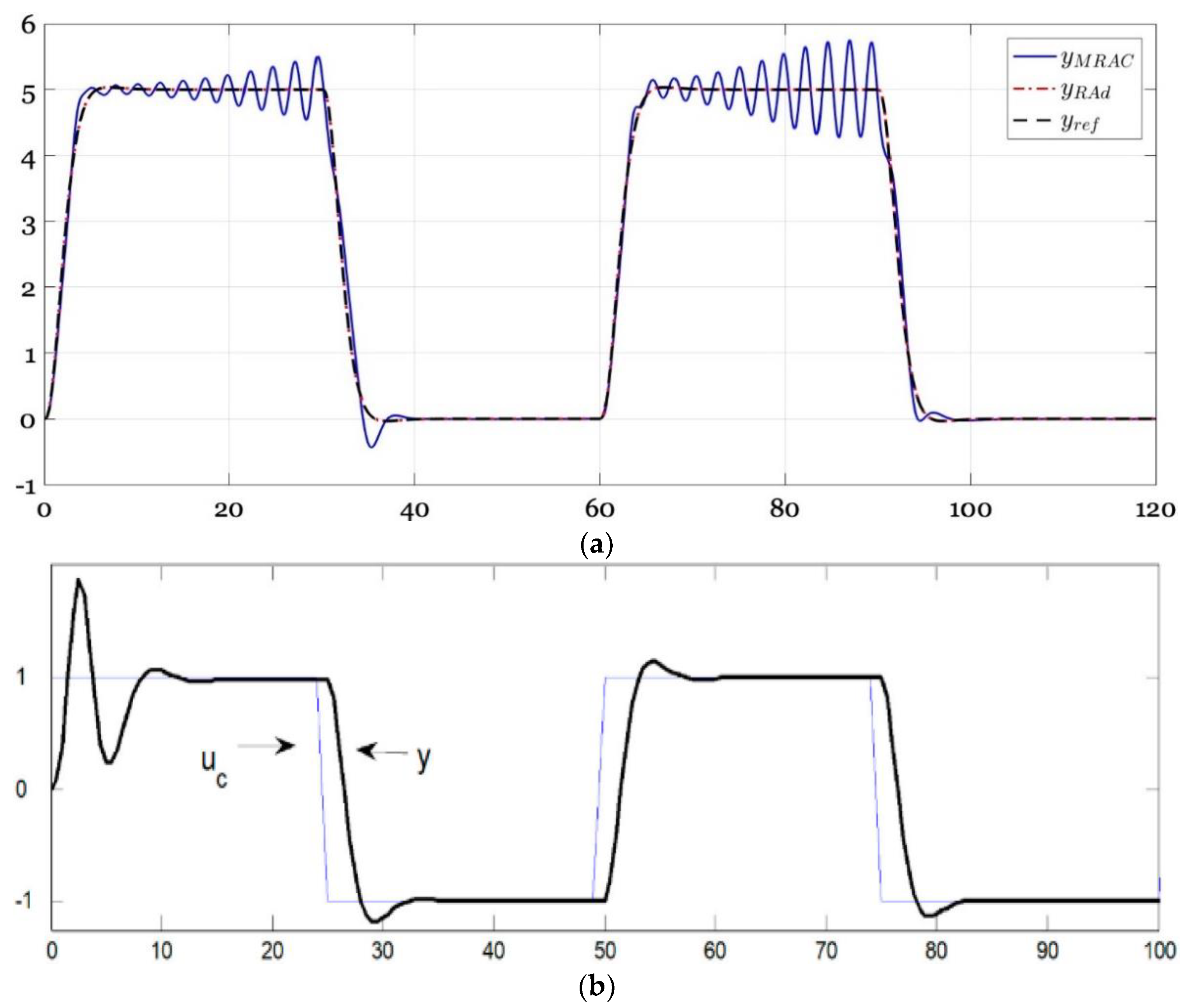
(a) Comparison of model reference adaptive control and robust adaptive control tracking square waves from [29]. Notice the square waves are rounded to reduce the deleterious challenge of discontinuity; (b) self-tuning regulators tracking square wave commands from [35]. Notice the square waves are not rounded, implying a relatively more challenging demand.
Figure 5.
(a) Comparison of model reference adaptive control and robust adaptive control tracking square waves from [29]. Notice the square waves are rounded to reduce the deleterious challenge of discontinuity; (b) self-tuning regulators tracking square wave commands from [35]. Notice the square waves are not rounded, implying a relatively more challenging demand.

Figure 6.
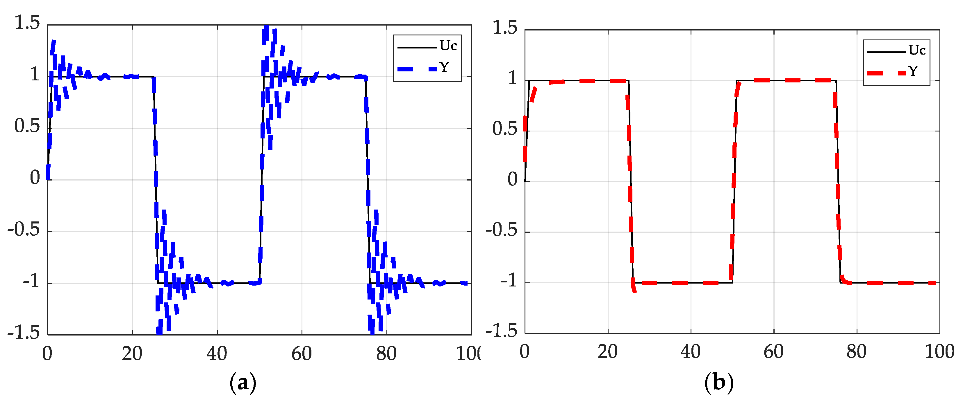
The output signals at a step-size of 0.50 s. (a) The black solid line describes the command signal. The blue dotted line (Left) represents the output signal generated by discrete D.A.I.; (b) the red dotted line (Right) describes the output signal generated by model-following method coupled with R.L.S. estimation.
Figure 6.
The output signals at a step-size of 0.50 s. (a) The black solid line describes the command signal. The blue dotted line (Left) represents the output signal generated by discrete D.A.I.; (b) the red dotted line (Right) describes the output signal generated by model-following method coupled with R.L.S. estimation.

Figure 7.
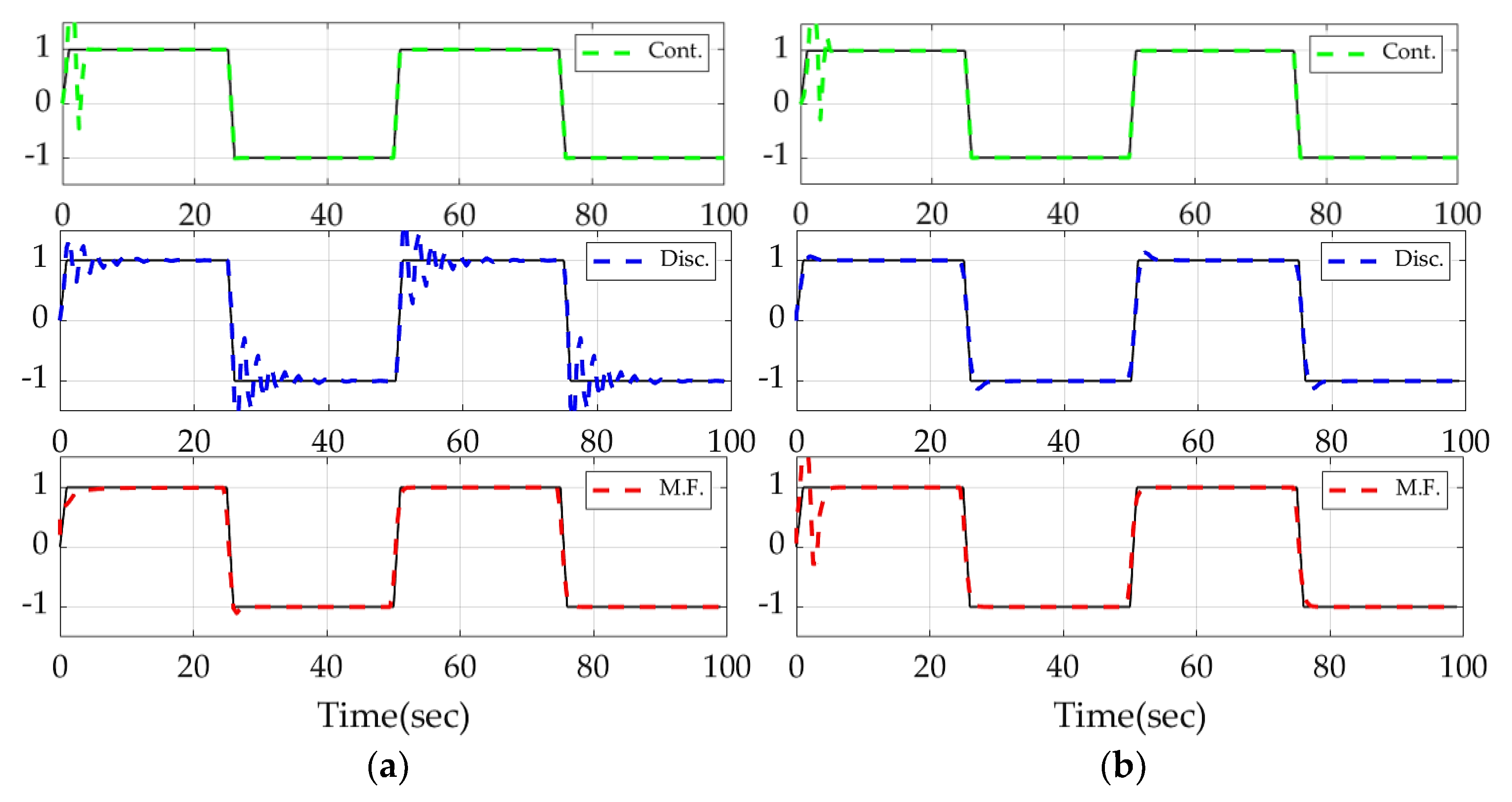
The output signals generated by all modeling approaches at step-sizes of 0.50 and 0.27 s. The detailed figure schemes for (a) and (b) follow the previous descriptions provided under Figure 1 and Figure 2.


Table 1.
Error distribution of D.A.I. and model-following method (M.F.) at varying step-sizes.
| Method | Step-Size [s] | Error Mean | Error Standard Deviation |
|---|---|---|---|
| D.A.I. | 0.50 | 0.0956 | 0.1632 |
| M.F. | 0.50 | 0.0278 | 0.0918 |
| D.A.I. | 0.27 | 0.0175 | 0.0545 |
| M.F. | 0.27 | 0.0471 | 0.1745 |
Table 2.
Error distribution of discrete D.A.I. and continuous D.A.I. at varying step-sizes.
| Type | Step-Size [s] | Error Mean | Error Std. |
|---|---|---|---|
| Discrete | 0.50 | 0.0956 | 0.1632 |
| Continuous | 0.50 | 0.0223 | 0.1654 |
| Discrete | 0.27 | 0.0175 | 0.0545 |
| Continuous | 0.27 | 0.0169 | 0.1397 |
Table 3.
Comparison of different discretization methods in discrete D.A.I.
| Discretization Method | Step-Size [s] | Error Mean | Error Standard Deviation |
|---|---|---|---|
| Matched | 0.50 | 0.0956 (0%) | 0.1632 (0%) |
| ZOH | 0.50 | 0.0730 (−24%) | 0.1317 (−19%) |
| Tustin FOH | 0.50 0.50 | 0.0204 (−79%) 0.0141 (−85%) | 0.0525 (−68%) 0.0330 (−80%) |
Table 4.
Percent performance improvement for D.A.I. and model-following adaptive control.
| Method | Step-Size [s] | Error Mean | Error Standard Deviation |
|---|---|---|---|
| D.A.I. | 0.50 | 0% | 0% |
| M.F. | 0.50 | −71% | −44% |
| D.A.I. | 0.27 | −82% | −67% |
| M.F. | 0.27 | −51% | 7% |
Table 5.
Percent performance improvement for continuous and discrete D.A.I.
| Method | Step-Size [s] | Error Mean | Error Standard Deviation |
|---|---|---|---|
| Discrete | 0.50 | 0% | 0% |
| Continuous | 0.50 | −77% | 1% |
| Discrete | 0.27 | −82% | −67% |
| Continuous | 0.27 | −82% | −14% |
Publisher’s Note: MDPI stays neutral with regard to jurisdictional claims in published maps and institutional affiliations. |
© 2022 by the authors. Licensee MDPI, Basel, Switzerland. This article is an open access article distributed under the terms and conditions of the Creative Commons Attribution (CC BY) license (https://creativecommons.org/licenses/by/4.0/).
Share and Cite
MDPI and ACS Style
Koo, S.M.; Travis, H.; Sands, T. Impacts of Discretization and Numerical Propagation on the Ability to Follow Challenging Square Wave Commands. J. Mar. Sci. Eng. 2022, 10, 419. https://doi.org/10.3390/jmse10030419
AMA Style
Koo SM, Travis H, Sands T. Impacts of Discretization and Numerical Propagation on the Ability to Follow Challenging Square Wave Commands. Journal of Marine Science and Engineering. 2022; 10(3):419. https://doi.org/10.3390/jmse10030419
Chicago/Turabian StyleKoo, Sung Mo, Henry Travis, and Timothy Sands. 2022. "Impacts of Discretization and Numerical Propagation on the Ability to Follow Challenging Square Wave Commands" Journal of Marine Science and Engineering 10, no. 3: 419. https://doi.org/10.3390/jmse10030419
Note that from the first issue of 2016, this journal uses article numbers instead of page numbers. See further details here.