Sensor Selection for Optimal Target localization with 3-D Angle of Arrival Estimation in Underwater Wireless Sensor Networks

Abstract

This paper investigates a sensor selection scheme for optimal target localization with three-dimensional (3-D) Angle of Arrival (AOA) estimation in Underwater Wireless Sensor Networks (UWSN). Specifically, we present a new 3-D AOA-based localization measurement model, which considers correlated noises and Gaussian priors. The trace of Cramer–Rao lower bound (CRLB) for the 3-D AOA measurement model is derived by introducing a special vector to denote the selected sensors with the azimuth and elevation angle measurements. Based on the presenting expressions of the CRLB, we formulate the sensor selection problem as an optimization problem, which has been transformed into the semidefinite problem program by convex relaxation, and a randomization method is adopted to improve the quality of the SDP solution. Simulation results illustrate that the proposed method receives better estimation performance over the reference methods and approaches the exhaustive search method.

1. Introduction

Underwater Wireless Sensor Network (UWSN) has become an active research area in recent years [1,2] and it has many potential applications in underwater security [3], ocean resource exploration [4], etc. One important research direction for UWSN is the target localization, as UWSN can provide much wider coverage with reasonable performance under the existing physical limitations of each sensor. The localization methods calculate the target location using various parameter measurement from each individual sensor [5], such as the Time-Of-Arrival (TOA) [6], the Time-Difference-of-Arrival (TDOA) [7], the Angle-Of-Arrival (AOA) [8], the Received Signal Strength (RSS) [9], etc. Among these, the AOA-based localization method requires relatively less data exchange (angle-only) and lower hardware support [10], as it does not rely on the time synchronization. In turn, many recent works show that it appears to be a promising technique in real applications [11,12,13,14,15,16]. The main contributions in this direction are mainly focused on the inaccurate sensor location [11], the angle estimation robustness [12,13], and the time-variant acoustic propagation path [14], and the sensor selection [15,16].

The sensor selection is an important process in the UWSN application, as it is impractical to use all sensors for localization due to the large detection range and the target signal transmission loss. In addition, the usage of the sensors is also constrained by the hardware costs, data storage space, and sensor battery life in the underwater scenarios. The purpose of sensor selection is to find a group of sensors that are the most necessary ones to obtain the optimal localization performance and, at the same time, the balance between the estimation accuracy and the number of activated sensors [17,18].

Sensor selection problem is always formulated as an optimization problem based on two commonly used criteria: to minimize the trace of the Cramér–Rao lower bound (CRLB) and to maximize the determinant of the Fisher information matrix (FIM). The sensor selection problem can be formulated as an integer programming (IP) problem under these criteria, and one Boolean vector is defined as an indicator to indicate the selected sensors. However, the IP problem is a NP-hard problem and difficult to solve. The straightforward method to obtain the optimal subset is to enumerate all the possible sensor combinations and select the optimal performance sensor subset, which is known as the exhaustive search method. However, this method is computationally intensive and does not apply in a practical environment. Consequently, many suboptimal methods have been proposed, including the convex optimization and other heuristic algorithms. Two heuristic methods, named “iterative swapping greedy (ISG)” and “best option filling (BOF)”, can also be used to obtain an optimal solution. Although the two methods have comparable performance with the SDR method, they still have the risk of local convergence. Thus, most literature dealt with the sensor selection problem by convex relaxation that relaxes the original nonconvex problem as a semidefinite program (SDP).

In [19,20], a convex optimization method was proposed for sensor selection, a linear measurement model was used and the problems were solved approximately by convex relaxation. Based on them, a sparsity promoting method for sensor selections aimed to minimize the number of selected sensors under a constraint on the target state estimation error in [21,22]. However, in the existing literature, the research of sensor selection problem hinges on the assumption of uncorrelated measurement noises. Later, the proposed sensor selection framework was valid for an arbitrary noise correlation matrix in [23], and then the authors in [24] considered a more complex scenario with correlated measurement noise, which was designed for sparse signal estimation, yet it is not suitable for three-dimensional space. In the aforementioned literature, some works on the following aspects has not been carried out. In 3-D space, the sensor selection problem becomes more challenging due to the increased size of the Fisher information matrix (two measurements: the azimuth angle and elevation angle), yet the existing AOA-based sensor selection method for 2-D space is not suitable for 3-D space [25]. Furthermore, currently most of the literature on sensor selection normally assumed that the measurement noises of the sensors are ideally uncorrelated [16,17,18,19,20,21,22]. However, in a dynamic marine environment with a similar acoustic background and sound propagation path, this assumption may not be satisfied [26]. Although the authors in [23] have studied the sensor selection with correlated measurement noises, yet it is not designed for 3-D space, and thus not suitable for the UWSN.

Motivated by the observations above, in this paper, we focus on the sensor selection problem using the 3-D AOA-based localization with correlated measurement noise in UWSN. The main contributions of this paper are outlined as follows:

• In order to solve the AOA-based sensor selection problem in 3-D space, we propose a novel sensor selection method and introduce one Boolean vector with the azimuth angle and elevation angle measurements under correlated noises.
• A sensor selection problem is formulated as an optimization problem by minimizing the CRLB for the 3-D AOA-based localization. The SDR solution is utilized to transform the optimization problem as convex SDPs, and then a randomization method is used to refine the quality of the SDP solution.
• Simulation studies are presented to verify whether the proposed method can outperform the other methods and achieve the performance of the exhaustive search method at the cost of much lower complexity.

The rest of this paper is organized as follows: The 3-D AOA sensor selection problem with the correlated measurement noise is formulated in Section 2. Section 3 develops the nonconvex sensor selection optimization problem. The basic convex relaxation and a randomization method are described in Section 4. Section 5 presents the comprehensive simulation results, and the conclusion is drawn in Section 6.

2. Problem Formulation

In this paper, we consider a 3-D underwater sensor network that is composed of N distributed sensors with a stationary target, where ${\mathbf{p}}_k={\left(p_{xk},p_{yk},p_{zk}\right)}^T,k=1,2,\cdots N$ is the location of the sensors with ${}^T$ denoting matrix transpose. $\mathbf{s}={\left(x,y,z\right)}^T$ is the unknown location of the target, it is assumed that $\mathbf{s}$ is a Gaussian random variable with a distribution as $\mathbf{s}\sim \mathcal{N}\left({\mathbf{s}}_0,{\mathbf{P}}_0\right)$, where ${\mathbf{s}}_0$ and ${\mathbf{P}}_0$ represent the mean and the covariance matrix of $\mathbf{s}$. Note that each sensor can acquire the bearing measurement with azimuth and elevation angles in spherical coordinates, which can be utilized to localize the unknown target in the marine scenarios. The measurement model of the $k\mathrm{th}$ sensor can be expressed as [27]

$$\begin{array}{c}\hfill \begin{array}{c}\hfill {\tilde{f}}_k=f_k+{\alpha }_k={\phi }_k\left(\mathbf{s},{\mathbf{p}}_k\right)+{\alpha }_k,\end{array}\end{array}$$

(1)

where ${\phi }_k\left(\mathbf{s},{\mathbf{p}}_k\right)$ is the noise-free measurement which is a nonlinear function of $\mathbf{s}$ and ${\mathbf{p}}_k$, and ${\alpha }_k$ denotes the measurement noise. Using ${\tilde{\phi }}_k$ for $k=1,\cdots ,N$ and the vector form of the measurement model is given by

$$\begin{array}{c}\hfill \begin{array}{c}\hfill \tilde{\mathbf{f}}=\mathbf{f}+\mathbf{\alpha },\end{array}\end{array}$$

(2)

with

$$\begin{array}{c}\hfill \begin{array}{cc}\hfill & \tilde{\mathbf{f}}={\left[{\tilde{f}}_1,\cdots ,{\tilde{f}}_N\right]}^T,\hfill \\ \hfill & \mathbf{f}={\left[f_1,\cdots ,f_N\right]}^T={\left[{\phi }_1\left(\mathbf{s},{\mathbf{p}}_1\right),\cdots ,{\phi }_N\left(\mathbf{s},{\mathbf{p}}_N\right)\right]}^T,\hfill \\ \hfill & \mathbf{\alpha }={\left[{\alpha }_1,\cdots ,{\alpha }_N\right]}^T.\hfill \end{array}\end{array}$$

(3)

$\mathbf{\alpha }$ is the measurement noise vector with a Gaussian distribution $\mathcal{N}\left(0,{\sigma }_{\alpha }^2{\mathbf{R}}_{\alpha }\right)$. Here, ${\sigma }_{\alpha }^2$ is the noise variance, and the matrix ${\mathbf{R}}_{\alpha }$ is not diagonal due to the noise measurements may be correlated among different sensors [25]. It is assumed that ${\mathbf{R}}_{\alpha }$ is an autoregressive matrix and each element ${\mu }_{i,j}$ (row is i and column is j, $0\le \mu <1$) denotes the correlation coefficient. Thus, the matrix ${\mathbf{R}}_{\alpha }$ can be used for modeling noise correlations between distributed sensors in marine scenarios.

In the 3-D space, the AOA-based localization measurement becomes more challenging because of the increase in the size of the FIM from $2\times 2$ to $3\times 3$, making the optimality analysis more cumbersome. Hence, the azimuth and elevation angle measurement models are introduced, respectively.

Using ${\mathbf{s}}_0={\left(x_0,y_0,z_0\right)}^T$ as a reference, and $\left\{{\theta }_k,{\varphi }_k\right\}$ denotes the bearing measurement with azimuth and elevation angle in spherical coordinates [28]. The azimuth angle measurement of the $k\mathrm{th}$ sensor, takes the form

$$\begin{array}{c}\hfill \begin{array}{c}\hfill f_k={\phi }_k\left({\mathbf{s}}_0,{\mathbf{p}}_k\right)={\theta }_k={tan}^{-1}\frac{y_0-p_{yk}}{x_0-p_{xk}},-\pi <\theta \le \pi ,\end{array}\end{array}$$

(4)

where ${tan}^{-1}$ is the 4-quadrant arctangent, $\mathbf{f}={\left[f_1,\cdots ,f_N\right]}^T={\left[{\theta }_1,\cdots ,{\theta }_N\right]}^T$, and we assume that $\mathbf{\beta }={\left[{\beta }_1,\cdots ,{\beta }_N\right]}^T$ is the azumuth angle measurement noise vector following Gaussian distribution $\mathbf{\beta }\sim \mathcal{N}\left(0,{\sigma }_{\theta }^2{\mathbf{R}}_{\theta }\right)$.

The elevation angle measurement of the $k\mathrm{th}$ sensor, we obtain

$$\begin{array}{c}\hfill \begin{array}{c}\hfill f_k={\phi }_k\left({\mathbf{s}}_0,{\mathbf{p}}_k\right)={\varphi }_k={sin}^{-1}\frac{z_0-p_{zk}}{r_k},-\frac{\pi }{2}<\varphi \le \frac{\pi }{2},\end{array}\end{array}$$

(5)

where $r_k=∥{\mathbf{s}}_0-{\mathbf{p}}_k∥$, $∥·∥$ denotes the Euclidean norm, $\mathbf{f}={\left[f_1,\cdots ,f_N\right]}^T={\left[{\varphi }_1,\cdots ,{\varphi }_N\right]}^T$, and we assume that $\mathbf{\gamma }={\left[{\gamma }_1,\cdots ,{\gamma }_N\right]}^T$ is the elevation angle measurement noise vector following Gaussian distribution $\mathbf{\gamma }\sim \mathcal{N}\left(0,{\sigma }_{\varphi }^2{\mathbf{R}}_{\varphi }\right)$. Here, we denote the 3-D AOA-based measurement noise vector as

$$\begin{array}{c}\hfill \begin{array}{c}\hfill \mathbf{\zeta }=\left[\mathbf{\beta },\mathbf{\gamma }\right],\end{array}\end{array}$$

(6)

Thus, the measurement noise covariance matrix of the N sensors with $2N$ measurements can be written as

$$\begin{array}{c}\hfill \begin{array}{c}\hfill \mathsf{\Sigma }=\mathbb{E}\left\{\mathbf{\zeta }{\mathbf{\zeta }}^T\right\}=\mathrm{diag}\left\{{\sigma }_{\theta }^2{\mathbf{R}}_{\theta },{\sigma }_{\varphi }^2{\mathbf{R}}_{\varphi }\right\},\end{array}\end{array}$$

(7)

where ${\sigma }_{\theta }^2$ and ${\sigma }_{\varphi }^2$ are the azimuth and elevation angle noise variance, and the matrix ${\mathbf{R}}_{\theta }$ and ${\mathbf{R}}_{\varphi }$ are not diagonal due to the noise measurements may be correlated among different sensors. It is assumed that ${\mathbf{R}}_{\theta }$ and ${\mathbf{R}}_{\varphi }$ are autoregressive matrices and each element ${\mu }_{i,j}$ (row is i and column is j, $0\le \mu <1$) denotes the correlation coefficient.

The Jacobian matrix of the $2N$ measurements is given [28]

$$\begin{array}{c}\hfill \begin{array}{cc}\hfill \mathbf{J}& =\left[\begin{array}{ccc}-{\displaystyle \frac{sin{\theta }_1}{r_{1}cos{\varphi }_1}}& {\displaystyle \frac{cos{\theta }_1}{r_{1}cos{\varphi }_1}}& 0\\ ⋮& ⋮& ⋮\\ -{\displaystyle \frac{sin{\theta }_N}{r_{N}cos{\varphi }_N}}& {\displaystyle \frac{cos{\theta }_N}{r_{N}cos{\varphi }_N}}& 0\\ -{\displaystyle \frac{sin{\varphi }_{1}cos{\theta }_1}{r_1}}& -{\displaystyle \frac{sin{\varphi }_{1}sin{\theta }_1}{r_1}}& {\displaystyle \frac{cos{\varphi }_1}{r_1}}\\ ⋮& ⋮& ⋮\\ -{\displaystyle \frac{sin{\varphi }_{N}cos{\theta }_N}{r_N}}& -{\displaystyle \frac{sin{\varphi }_{N}sin{\theta }_N}{r_N}}& {\displaystyle \frac{cos{\varphi }_N}{r_N}}\end{array}\right],\hfill \end{array}\end{array}$$

(8)

The FIM for 3-D AOA localization with Gaussian problem yields

$$\begin{array}{c}\hfill \begin{array}{c}\hfill \mathbf{FIM}={\mathbf{P}}_0^{-1}+{\mathbf{J}}^T{\mathsf{\Sigma }}^{-1}\mathbf{J},\end{array}\end{array}$$

(9)

and

$$\begin{array}{c}\hfill \begin{array}{c}\hfill \mathbf{CRLB}={\mathbf{FIM}}^{-1}.\end{array}\end{array}$$

(10)

Next, we consider the sensor selection problem, which chooses the best subset from the sensor network to achieve the best localization accuracy. We are motivated to select the best subset with M sensors of N ($N>M$) active sensors that minimize the localization error, subject to a constraint on the number of active sensors. However, one 3-D AOA-based sensor is determined by azimuth and elevation angle measurements. Hence, we should select two measurement equations for the same sensor. For this reason, we introduce a Boolean vector:

$$\begin{array}{c}\hfill \begin{array}{c}\hfill \mathbf{r}={\left[\begin{array}{cc}{\mathbf{w}}^T,& {\mathbf{v}}^T\end{array}\right]}^T,\end{array}\end{array}$$

(11)

where $\mathbf{w}$ denotes the sensor selection vector for the azimuth angle measurement, and $\mathbf{v}$ represents the sensor selection vector for the elevation angle measurement, respectively.

$$\begin{array}{c}\hfill \begin{array}{cc}\hfill & \mathbf{w}={\left[w_1,w_2,\cdots ,w_N\right]}^T,w_i\in \left\{0,1\right\},i=1,2,\cdots ,N,\hfill \\ \hfill & \mathbf{v}={\left[v_1,v_2,\cdots ,v_N\right]}^T,v_j\in \left\{0,1\right\},i=1,2,\cdots ,N,\hfill \end{array}\end{array}$$

(12)

$w_i$ and $v_j$ indicate whether or not the $i\mathrm{th}$ sensor is selected by the azimuth angle measurement and the elevation angle measurement, respectively.

We define two matrices ${\mathsf{\Phi }}_w$ (${\mathsf{\Phi }}_w\in {\mathbb{R}}^{M\times N}$) and ${\mathsf{\Phi }}_v$ (${\mathsf{\Phi }}_v\in {\mathbb{R}}^{M\times N}$), which are related to Boolean selection vectors. ${\mathsf{\Phi }}_w$ is a submatrix of $\mathrm{diag}\left(\mathbf{w}\right)$ ($\mathrm{diag}\left(\mathbf{w}\right)\in {\mathbb{R}}^{N\times N}$) after all rows corresponding to the unselected sensors have been removed, and the diagonal entries of $\mathrm{diag}\left(\mathbf{w}\right)$ are formed by $\mathbf{w}$, and ${\mathsf{\Phi }}_v$ is expanded by $\mathbf{v}$, respectively. Therefore, we can get the link of them as below:

$$\begin{array}{c}\hfill \begin{array}{cc}\hfill & {\mathsf{\Phi }}_w{\mathsf{\Phi }}_w^T={\mathbf{I}}_w,{\mathsf{\Phi }}_w^T{\mathsf{\Phi }}_w=\mathrm{diag}\left(\mathbf{w}\right),\hfill \\ \hfill & {\mathsf{\Phi }}_v{\mathsf{\Phi }}_v^T={\mathbf{I}}_v,{\mathsf{\Phi }}_v^T{\mathsf{\Phi }}_v=\mathrm{diag}\left(\mathbf{v}\right),\hfill \end{array}\end{array}$$

(13)

and

$$\begin{array}{c}\hfill \begin{array}{c}\hfill {\mathsf{\Phi }}_r{\mathsf{\Phi }}_r^T={\mathbf{I}}_r,{\mathsf{\Phi }}_r^T{\mathsf{\Phi }}_r=\mathrm{diag}\left(\mathbf{r}\right),\end{array}\end{array}$$

(14)

From the above definition, when the selected sensor subset is obtained, the noise covariance matrix can be expressed:

$$\begin{array}{c}\hfill \begin{array}{c}\hfill {\mathsf{\Sigma }}_r=\mathrm{E}\left[{\mathsf{\Phi }}_r\mathbf{\zeta }{\left({\mathsf{\Phi }}_r\mathbf{\zeta }\right)}^T\right]={\mathsf{\Phi }}_r{\mathsf{\Sigma }\mathsf{\Phi }}_r^T,\end{array}\end{array}$$

(15)

Thus, we can get the FIM for the selected sensor subset with the Gaussian prior distribution:

$$\begin{array}{c}\hfill \begin{array}{c}\hfill \mathbf{FI}{\mathbf{M}}_r={\mathbf{P}}_0^{-1}+{\mathbf{J}}^T{\mathsf{\Phi }}_r^T{\mathsf{\Sigma }}_r^{-1}{\mathsf{\Phi }}_r\mathbf{J}.\end{array}\end{array}$$

(16)

3. Sensor Selection Method for the 3-D AOA-Based Localization

In this section, we derive the sensor selection method for the 3-D AOA-based localization with correlated measurement noise. Firstly, we consider a decomposition of the azimuth and elevation angle noise covariance matrix, and then the sensor selection problem with correlated measurement noise can be formulated as an optimization problem. Moreover, the A-optimality criterion (minimizing the trace of the CRLB) is used as the optimization objective. The decomposition of the noise covariance matrix for azimuth and elevation angle measurements can be given by, respectively,

$$\begin{array}{c}\hfill \begin{array}{cc}\hfill & {\mathsf{\Sigma }}_{\theta }={\lambda }_{\theta }{\mathbf{I}}_N+{\mathbf{Z}}_{\theta },\hfill \\ \hfill & {\mathsf{\Sigma }}_{\varphi }={\lambda }_{\varphi }{\mathbf{I}}_N+{\mathbf{Z}}_{\varphi },\hfill \end{array}\end{array}$$

(17)

where ${\lambda }_{\theta }$, ${\lambda }_{\varphi }$ are positive scalars to ensure ${\mathbf{Z}}_{\theta }$, ${\mathbf{Z}}_{\varphi }$ are positive definite matrices, and $\mathbf{I}$ is the identity matrix. Thus, we can obtain the decomposition of the noise covariance matrix for the 3-D AOA measurement as

$$\begin{array}{c}\hfill \begin{array}{c}\hfill \mathsf{\Sigma }=\mathsf{\Gamma }+\mathbf{Z},\end{array}\end{array}$$

(18)

and $\mathsf{\Gamma }=\mathrm{diag}\{{\lambda }_{\theta }{\mathbf{I}}_N,{\lambda }_{\varphi }{\mathbf{I}}_N\}$, $\mathbf{Z}=\mathrm{diag}\{{\mathbf{Z}}_{\theta },{\mathbf{Z}}_{\varphi }\}$. Substituting (18) into (15), we get

$$\begin{array}{c}\hfill \begin{array}{c}\hfill {\mathsf{\Sigma }}_r={\mathsf{\Phi }}_r\left(\mathsf{\Gamma }+\mathbf{Z}\right){\mathsf{\Phi }}_r^T={\mathsf{\Gamma }}_r+{\mathsf{\Phi }}_r{\mathbf{Z}\mathsf{\Phi }}_r^T,\end{array}\end{array}$$

(19)

and ${\mathsf{\Gamma }}_r=\mathrm{diag}\{{\lambda }_{\theta }{\mathbf{I}}_M,{\lambda }_{\varphi }{\mathbf{I}}_M\}$.

Using (19), the second part of the right-hand side of (16) can be expressed as

$$\begin{array}{c}\hfill \begin{array}{cc}\hfill {\mathsf{\Phi }}_r^T{\mathsf{\Sigma }}_r^{-1}{\mathsf{\Phi }}_r& ={\mathsf{\Phi }}_r^T{\left({\mathsf{\Gamma }}_r+{\mathsf{\Phi }}_r{\mathbf{Z}\mathsf{\Phi }}_r^T\right)}^{-1}{\mathsf{\Phi }}_r,\hfill \end{array}\end{array}$$

(20)

By using the matrix inversion lemma [29], for matrices $\mathbf{A}$, $\mathbf{B}$, $\mathbf{C}$, and $\mathbf{D}$, the matrix inversion lemma states that ${\left(\mathbf{A}+\mathbf{BCD}\right)}^{-1}={\mathbf{A}}^{-1}-{\mathbf{A}}^{-1}\mathbf{B}{\left({\mathbf{C}}^{-1}+\mathbf{D}{\mathbf{A}}^{-1}\mathbf{B}\right)}^{-1}\mathbf{D}{\mathbf{A}}^{-1}$, which yields $\mathbf{B}{\left({\mathbf{C}}^{-1}+\mathbf{D}{\mathbf{A}}^{-1}\mathbf{B}\right)}^{-1}\mathbf{D}=\mathbf{A}-\mathbf{A}{\left(\mathbf{A}+\mathbf{BCD}\right)}^{-1}\mathbf{A}$, with $\mathbf{A}={\mathbf{Z}}^{-1},\mathbf{B}={\mathsf{\Phi }}_r^T,$$\mathbf{C}={\mathsf{\Gamma }}_r,$$\mathbf{D}={\mathsf{\Phi }}_r$, and ${\mathsf{\Phi }}_r^T{\mathsf{\Phi }}_r=\mathrm{diag}\left(\mathbf{r}\right)$, the (20) can become

$$\begin{array}{c}\hfill \begin{array}{cc}\hfill {\mathsf{\Phi }}_r^T{\mathsf{\Sigma }}_r^{-1}{\mathsf{\Phi }}_r& ={\mathsf{\Phi }}_r^T{\left({\mathsf{\Gamma }}_r+{\mathsf{\Phi }}_r{\mathbf{Z}\mathsf{\Phi }}_r^T\right)}^{-1}{\mathsf{\Phi }}_r\hfill \\ \hfill & ={\mathbf{Z}}^{-1}-{\mathbf{Z}}^{-1}{\left({\mathbf{Z}}^{-1}+{\mathsf{\Gamma }}_r^{-1}{\mathsf{\Phi }}_r^T{\mathsf{\Phi }}_r\right)}^{-1}{\mathbf{Z}}^{-1}\hfill \\ \hfill & ={\mathbf{Z}}^{-1}-{\mathbf{Z}}^{-1}{\left({\mathbf{Z}}^{-1}+{\mathsf{\Gamma }}_r^{-1}\mathrm{diag}\left(\mathbf{r}\right)\right)}^{-1}{\mathbf{Z}}^{-1},\hfill \end{array}\end{array}$$

(21)

Substituting (21) into (16), it derives

$$\begin{array}{c}\hfill \begin{array}{cc}\hfill \mathbf{FI}{\mathbf{M}}_r=& {\mathbf{P}}_0^{-1}+{\mathbf{J}}^T{\mathbf{Z}}^{-1}\mathbf{J}\hfill \\ \hfill & -{\mathbf{J}}^T{\mathbf{Z}}^{-1}{\left({\mathbf{Z}}^{-1}+{\mathsf{\Gamma }}_r^{-1}\mathrm{diag}\left(\mathbf{r}\right)\right)}^{-1}{\mathbf{Z}}^{-1}\mathbf{J}.\hfill \end{array}\end{array}$$

(22)

Using (22), we can explicitly establish the relationship between $\mathbf{FI}{\mathbf{M}}_r$ and $\mathbf{r}$. Since the A-optimality criterion, i.e., minimizing the $\mathrm{tr}\left(\mathbf{FI}{\mathbf{M}}_r^{-1}\right)$, is equivalent to minimize the mean squared error (MSE) estimation directly, which is used as the objective function. Hence, the optimization problem of the sensor selection can be formulated as

$$\begin{array}{c}\hfill \begin{array}{cc}\hfill & \begin{array}{cc}\underset{\mathbf{r}}{\min }& \mathrm{tr}\left({\mathbf{FIM}}_r^{-1}\right)\end{array}\hfill \\ \hfill & \begin{array}{cc}\mathrm{s}.\mathrm{t}.& 1^T\mathbf{r}=2M,\\ & \mathbf{r}\in {\left\{0,1\right\}}^{2N}.\end{array}\hfill \end{array}\end{array}$$

(23)

Note that (23) is a non-convex optimization problem due to the presence of the Boolean selection variables. In what follows, we will transform the original non-convex problem into the semidefinite problem program (SDP) by convex relaxation.

4. Semidefinite Relaxation for Sensor Selection Problem

The sensor selection problem is described by the optimization problem in last section. Nevertheless, the original problem is a non-convex and NP-hard problem, which is difficult to solve. We propose a convex relaxation approach for the sensor selection problem with the correlated measurement noise. In addition, we also adopt a randomization method to improve the performance of the SDP method.

4.1. Sensor Selection Based on Semidefinite Relaxation Method

We define $\mathbf{A}={\mathbf{P}}_0^{-1}+{\mathbf{J}}^T{\mathbf{Z}}^{-1}\mathbf{J}$ and $\mathbf{B}={\mathbf{Z}}^{-1}\mathbf{J}$ in (22) for the notational simplicity, thus, the equivalent transformation (23) can be given by

$$\begin{array}{c}\hfill \begin{array}{cc}\hfill & \begin{array}{cc}\underset{\mathbf{r}}{\min }& \mathrm{tr}\left(\mathbf{X}\right)\end{array}\hfill \\ \hfill & \begin{array}{cc}\mathrm{s}.\mathrm{t}.& \mathbf{A}-\end{array}{\mathbf{B}}^T{\left({\mathbf{Z}}^{-1}+{\mathsf{\Gamma }}_r^{-1}\mathrm{diag}\left(\mathbf{r}\right)\right)}^{-1}\mathbf{B}\succcurlyeq {\mathbf{X}}^{-1},\hfill \\ \hfill & \begin{array}{cc}& 1^T\mathbf{r}=2M,\\ & \mathbf{r}\in {\left\{0,1\right\}}^{2N}.\end{array}\hfill \end{array}\end{array}$$

(24)

where $\mathbf{X}\in {\mathbb{R}}^{M\times M}$ is an auxiliary variable with symmetric structure, and $\mathbf{U}\le \mathbf{V}$ (or $\mathbf{U}\ge \mathbf{V}$) denote $\mathbf{V}-\mathbf{U}$ (or $\mathbf{U}-\mathbf{V}$) is the positive semidefinite matrix. By using the Schurs complement, the first inequality constraint (24) can be expressed as [21]

$$\begin{array}{c}\hfill \begin{array}{c}\hfill \left(\mathbf{A}-{\mathbf{B}}^T{\left({\mathbf{Z}}^{-1}+{\mathsf{\Gamma }}_r^{-1}\mathrm{diag}\left(\mathbf{r}\right)\right)}^{-1}\mathbf{B}\right)\preccurlyeq \mathbf{X},\end{array}\end{array}$$

(25)

Lately, another variable $\mathbf{Y}\in {\mathbb{R}}^{M\times M}$ is introduced and the above inequality constraint equivalently is given as

$$\begin{array}{c}\hfill \begin{array}{c}\hfill \mathbf{A}-\mathbf{Y}\succcurlyeq {\mathbf{X}}^{-1},\end{array}\end{array}$$

(26)

with

$$\begin{array}{c}\hfill \begin{array}{c}\hfill \mathbf{Y}\succcurlyeq {\mathbf{B}}^T{\left({\mathbf{Z}}^{-1}+{\mathsf{\Gamma }}_r^{-1}\mathrm{diag}\left(\mathbf{r}\right)\right)}^{-1}\mathbf{B},\end{array}\end{array}$$

(27)

Note that using the inequalities (26) and (27) to minimize the $\mathrm{tr}\left(\mathbf{X}\right)$ can force the variable $\mathbf{Y}$ to reach its lower bound. Next, we can adopt the Schur complement to further decompose the first inequality constraint in (19) into two linear matrix inequalities (LMIs):

$$\begin{array}{c}\hfill \begin{array}{c}\hfill \left[\begin{array}{cc}\mathbf{A}-\mathbf{Y}& \mathbf{I}\\ \mathbf{I}& \mathbf{X}\end{array}\right]\succcurlyeq 0,\left[\begin{array}{cc}\mathbf{Y}& {\mathbf{B}}^T\\ \mathbf{B}& {\mathbf{Z}}^{-1}+{\mathsf{\Gamma }}_r^{-1}\mathrm{diag}\left(\mathbf{r}\right)\end{array}\right]\succcurlyeq 0,\end{array}\end{array}$$

(28)

Substituting (28) into (24), and the problem is expressed as

$$\begin{array}{c}\hfill \begin{array}{cc}\hfill & \begin{array}{cc}\underset{\mathbf{r},\mathbf{X},\mathbf{Y}}{\min }& \mathrm{tr}\left(\mathbf{X}\right)\end{array}\hfill \\ \hfill & \begin{array}{cc}\mathrm{s}.\mathrm{t}.& \mathrm{LMIs}\mathrm{in}\left(28\right),\\ & 1^T\mathbf{r}=2M,\\ & \mathbf{r}\in {\left\{0,1\right\}}^{2N}.\end{array}\hfill \end{array}\end{array}$$

(29)

Obviously, the above problem has the form of SDP except for the non-convex constraint of the Boolean selection vector $\mathbf{r}$. To tackle this difficulty, we substitute the convex $\mathbf{r}\in {\left[0,1\right]}^{2N}$ for nonconvex constraint $\mathbf{r}\in {\left\{0,1\right\}}^{2N}$. Thus, the problem (29) can be transformed to an SDP as

$$\begin{array}{c}\hfill \begin{array}{cc}\hfill & \begin{array}{cc}\underset{\mathbf{r},\mathbf{X},\mathbf{Y}}{\min }& \mathrm{tr}\left(\mathbf{X}\right)\end{array}\hfill \\ \hfill & \begin{array}{cc}\mathrm{s}.\mathrm{t}.& \mathrm{LMIs}\mathrm{in}\left(28\right),\\ & 1^T\mathbf{r}=2M,\\ & 0\le r_i\le 1,i=1,2,\cdots ,2N.\end{array}\hfill \end{array}\end{array}$$

(30)

The SDP problem can be solved easily and efficiently by using an interior point algorithm. When the fractional vector $\mathbf{r}$ is solved, we can extract $\mathbf{w}$ and $\mathbf{v}$ form it. The simplest method is to determine the maximal M weight value. Notably, the fractional vectors $\mathbf{w}$ and $\mathbf{v}$ are used to determine the sensor selection by the azimuth angle and elevation angle measurements, respectively. We can define a new fractional vector as

$$\begin{array}{c}\hfill \begin{array}{c}\hfill \mathbf{u}=\mathbf{w}+\mathbf{v}.\end{array}\end{array}$$

(31)

In the 3-D AOA-based scenario, the optimal sensor subset should be selected by the fractional vector $\mathbf{u}$. We can choose the maximal M weight from $\mathbf{u}$. In the rest of the paper, we call the above sensor selection method “SDP” since it is developed based on the SDP, to distinguish it from the other method proposed in the following subsection.

4.2. Sensor Selection Based on Semidefinite Relaxation with Randomization Method

We use a randomization method to improve the solution of the problem [19]. The randomization method can generate a set of random fraction vectors related to the SDP solution, and a set of random Boolean selection vectors is given. Substitute each vector into the objective function and choose a vector with the minimum value. The Boolean constraint (14) on the entries of $\mathbf{r}$, we can introduce two auxiliary variables $\mathbf{W}$ and $\mathbf{V}$ together with the rank-one constraint

$$\begin{array}{c}\hfill \begin{array}{c}\hfill \mathbf{W}=\mathbf{w}{\mathbf{w}}^T,\mathbf{V}=\mathbf{v}{\mathbf{v}}^T,\end{array}\end{array}$$

(32)

which also can be equivalent to

$$\begin{array}{c}\hfill \begin{array}{cc}\hfill & \mathrm{tr}\left(\mathbf{W}\right)\le M,\mathrm{diag}\left(\mathbf{W}\right)=\mathbf{w},\hfill \\ \hfill & \mathrm{tr}\left(\mathbf{V}\right)\le M,\mathrm{diag}\left(\mathbf{V}\right)=\mathbf{v}.\hfill \end{array}\end{array}$$

(33)

After relaxing the (non-convex) rank-one constraint (32) to $\mathbf{W}\succcurlyeq \mathbf{w}{\mathbf{w}}^T,\mathbf{V}\succcurlyeq \mathbf{v}{\mathbf{v}}^T$, we can obtain

$$\begin{array}{c}\hfill \begin{array}{cc}\hfill & \begin{array}{cc}\underset{\mathbf{w},\mathbf{v},\mathbf{W},\mathbf{V},\mathbf{X},\mathbf{Y}}{\min }& \mathrm{tr}\left(\mathbf{X}\right)\end{array}\hfill \\ \hfill & \begin{array}{cc}\mathrm{s}.\mathrm{t}.& \mathrm{LMIs}\mathrm{in}\left(\left(24\right)\right)\\ & \mathrm{tr}\left(\mathbf{W}\right)\le M,\mathrm{diag}\left(\mathbf{W}\right)=\mathbf{w},\\ & \mathrm{tr}\left(\mathbf{V}\right)\le M,\mathrm{diag}\left(\mathbf{V}\right)=\mathbf{v},\\ & \left[\begin{array}{cc}\mathbf{W}& \mathbf{w}\\ {\mathbf{w}}^T& 1\end{array}\right]\succcurlyeq 0,\left[\begin{array}{cc}\mathbf{V}& \mathbf{v}\\ {\mathbf{v}}^T& 1\end{array}\right]\succcurlyeq 0.\end{array}\hfill \end{array}\end{array}$$

(34)

We can first use an interior-point algorithm to solve the above SDP method, and then we adopt a randomization method to improve the quality of the above SDP solution. The SDP with randomization algorithm is as follows:

Step 1:

Generate two random vectors ${\mathbf{w}}_{\varsigma }^k\sim \mathcal{N}\left({\mathbf{w}}^O,{\mathbf{W}}_w-{\mathbf{w}}^o{{\mathbf{w}}^o}^T\right)$, ${\mathbf{v}}_{\varsigma }^k\sim \mathcal{N}\left({\mathbf{v}}^O,{\mathbf{V}}_w-{\mathbf{V}}^o{{\mathbf{V}}^o}^T\right)$, and $k=1,2,\dots ,N.$

Step 2:

For each sample, set the largest M elements as 1 and the rest as 0 to generate two feasible vectors ${\left({\mathbf{w}}_{\varsigma }^k\right)}_M$ and ${\left({\mathbf{v}}_{\varsigma }^k\right)}_M$, respectively.

Step 3:

Get the selected sensor index of the two vectors ${\left({\mathbf{w}}_{\varsigma }^k\right)}_M$ and ${\left({\mathbf{v}}_{\varsigma }^k\right)}_M$, that is, all the selected sensors of ${\left({\mathbf{w}}_{\varsigma }^k\right)}_M$ and ${\left({\mathbf{v}}_{\varsigma }^k\right)}_M$ as 1. Select the sensors have the same index (assume $a=1,\dots ,M$), and then, choose the $\left(M-a\right)$ sensors from the rest of “1” sensors.

Step 4:

Enumerate each possible combination to compute the objective function, and the minimum value of the sensor subset is selected.

Since the sensor selection method is developed based on the randomization method after the SDP is solved, we call it “SDP with randomization” in the rest of the paper.

4.3. Complexity Analysis

The SDP can be solved by the interior-point method in the polynomial time [29], and we first analyze the worst case complexities of the proposed method, and then compare with the exhaustive search method. From [30], the worst case complexity of solving an SDP is

$$\begin{array}{c}\hfill \begin{array}{c}\hfill \sqrt{\mu }\left(m^2\sum _{i=1}^{N_{SD}}{\left({\gamma }_i^{SD}\right)}^2+m\sum _{i=1}^{N_{SD}}{\left({\gamma }_i^{SD}\right)}^3+m^3\right)·ln\left(1/\epsilon \right),\end{array}\end{array}$$

(35)

where

$$\begin{array}{c}\hfill \begin{array}{c}\hfill \mu =\sum _{i=1}^{N_{SD}}{\gamma }_i^{SD},\end{array}\end{array}$$

(36)

m is the number of equality constraints, $N_{SD}$ is the number of semidefinite cone constrains, ${\gamma }_i^{SD}$ is the dimension of the ith semidefinite cone, and $\epsilon >0$ is the solution precision. The SDP (34) in the SDP method has about $N+2+{\left(2\times 2+2\right)}^2$ equality constraints, one semidefinite cone constraint $2\times \left(2\times 2+2\right)$, and one semidefinite cone constraint of size $2N+2$. Thus, the worst case complexity of solving (34) is on the order of $\mathcal{O}\left(N^{4.5}\right)·ln\left(1/\epsilon \right)$. The exhaustive search method enumerates all the possible sensor subset with size M from the sensor network with N sensors and calculates the CRLB. The total number of subsets is $\frac{N!}{\left(N-M\right)!M!}$, and the exhaustive search method demands extremely high computation complexity is $\mathcal{O}\left(N!\right)$. Obviously, the proposed method has a much lower computational complexity than the exhaustive search method.

5. Simulation Studies

In this section, simulations are presented to verify the performance of the proposed sensor selection method for the UWSN. For simplicity, we use “Exhaustive search” to denote the exhaustive search method, the method of the M closest sensors selected to the target is denoted by “Closest sensors”. We use “SDP” and “SDP with randomization” to denote the SDP solution without and with the randomization method, respectively. “All sensor” denotes all the sensors are activated to localize, and “Random selection” denotes the M sensors are selected at random.

In the following, we consider the sensor network with $N=40$ sensors are randomly placed in a underwater 3-D cube region of size $500\mathrm{m}\times 500\mathrm{m}\times 500\mathrm{m}$. It is assumed that the distribution of target is given, and ${\mathbf{s}}_0={\left(0,0,0\right)}^T$, ${\mathbf{P}}_0=\mathrm{diag}\left\{20,20,20\right\}$. For the proposed method, to guarantee a positive definite $\mathbf{Z}$ in (18), we set ${\lambda }_{\theta }={\lambda }_{\varphi }=0.9{\lambda }_{min}$, where ${\lambda }_{min}$ is the minimum eigenvalue of $\mathsf{\Sigma }$. Assuming that each sensor is omnidirectional, and this property can be achieved by the adoption of the circular array, the CRLB of the variance ${\sigma }_i^2$ [5]

$$\begin{array}{c}\hfill \begin{array}{c}\hfill {\sigma }_i^2\ge \mathrm{CRLB}\left(\mathrm{AOA}\right)={\displaystyle \frac{{\varphi }_{BW}^2}{{\mathrm{SNR}}_{\theta }}},\end{array}\end{array}$$

(37)

where ${\varphi }_{BW}$ is the effective beam width defined by ${\varphi }_{BW}={\displaystyle \frac{v}{\pi \rho k_{\mathrm{nrwms}}}}$, $\rho$ is the radius of the sensor array, v is the speed of propagation in length unit per sample, and define the normalized root weighted mean squared (nrwms) source frequency by

$$\begin{array}{c}\hfill \begin{array}{c}\hfill k_{\mathrm{nrwms}}={\displaystyle \frac{2}{L}}\sqrt{{\displaystyle \frac{{\sum }_{f=1}^{L/\phantom{L2}2}{f}^2{\left|S_s\left(f\right)\right|}^2}{{\sum }_{f=1}^{L/\phantom{L2}2}{f}^2{\left|S_s\left(f\right)\right|}^2}}}\end{array}\end{array}$$

(38)

L is the length of DFT, and $S_s\left(f\right)$ is the $L/\phantom{N2}2$ points DFT of the taget signal, the array SNR defined by [31]

$$\begin{array}{c}\hfill \begin{array}{c}\hfill \mathrm{SNR}=\frac{R}{L{\sigma }_n^2}{\sum }_{f=1}^{L/\phantom{L2}2}{\left|S_s\left(f\right)\right|}^2\end{array}\end{array}$$

(39)

where R is the number of sensor devices, and we assume that the ambient noise at each sensor node has the same variance ${\sigma }_n^2$.

We set the underwater average sound speed as $1500\mathrm{m}/\mathrm{s}$, $v=1500/1000=$$1.5\mathrm{m}/\mathrm{sample}$, $\rho =0.2\mathrm{m}$, $k_{\mathrm{nrwms}}=0.78$, $L=256$, $R=7$. Under this assumption, the variance ${\sigma }_{{\theta }_i}^2$ and ${\sigma }_{{\varphi }_i}^2$ can be calculated assuming the sensing devices in a circular array.

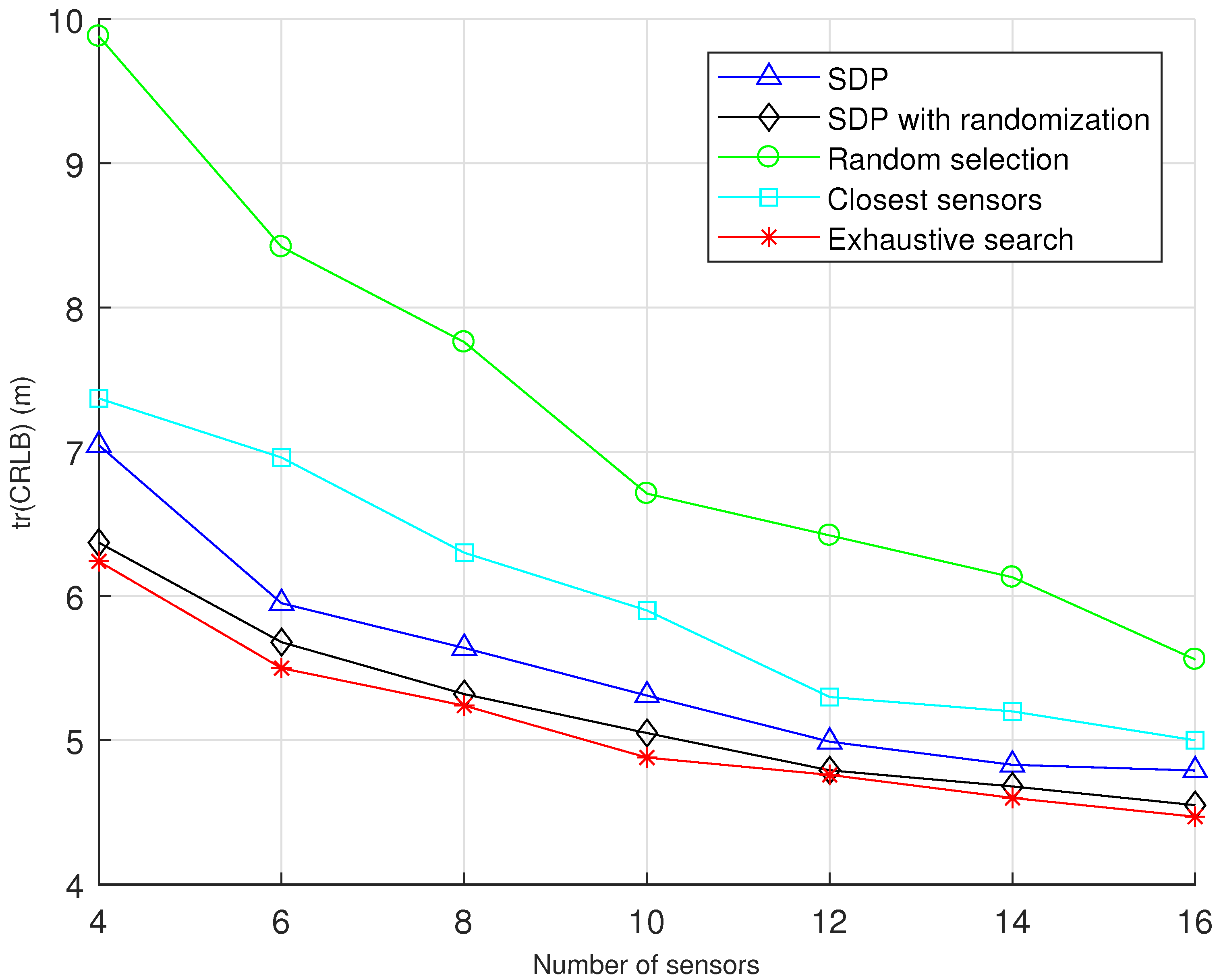
We firstly fix the signal to noise ratio of the azimuth and elevation angle as ${\sigma }_{{\theta }_1}^2=\cdots ={\sigma }_{{\theta }_N}^2={0.5}^{\circ }$, ${\sigma }_{{\varphi }_1}^2=\cdots ={\sigma }_{{\varphi }_N}^2={0.5}^{\circ }$. Figure 1 shows that the performance of the SDP methods without and with randomization when the $\mathrm{tr}\left(\mathrm{CRLB}\right)$ as M varies from 4 to 16. It can be seen that the results have a better estimation performance compared with the random selection method and the closest sensors. Besides, we adopt the exhaustive search that lists all possible sensor selection solutions to obtain the global optimum. We can observe that the $\mathrm{tr}\left(\mathrm{CRLB}\right)$ decreases significantly as the number of sensors increase. Furthermore, the proposed SDP method with randomization has a better estimation performance than the without randomization method, which also approaches the exhaustive search method.

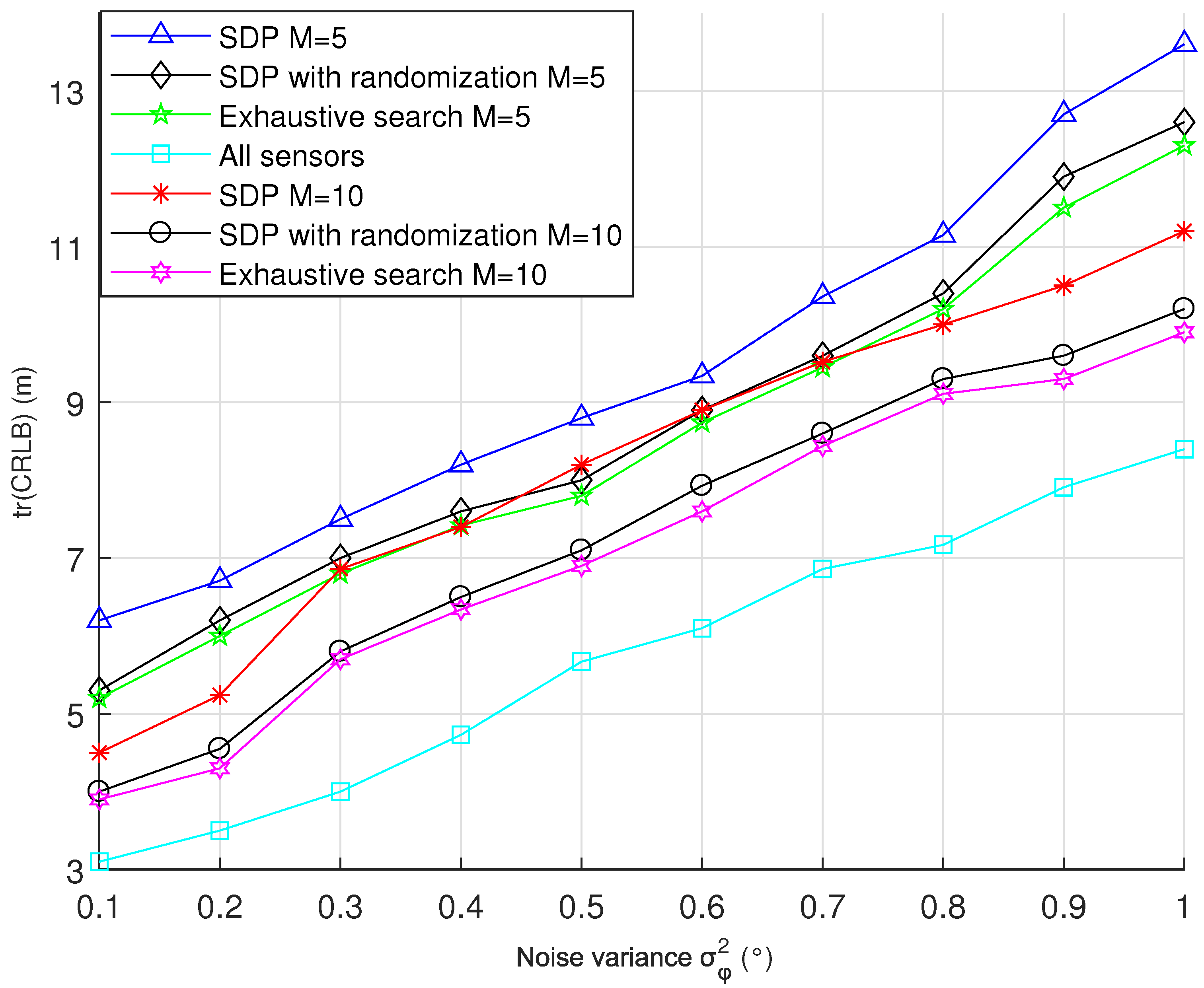
We next choose the number of selected sensors $M=5$ and $M=10$, and vary the noise variance. Figure 2 shows the $\mathrm{tr}\left(\mathrm{CRLB}\right)$ when ${\sigma }_{{\theta }_1}^2=\cdots ={\sigma }_{{\theta }_N}^2=1^{\circ }$, ${\sigma }_{{\varphi }_1}^2=\cdots ={\sigma }_{{\varphi }_N}^2={\sigma }_{{\varphi }_{}}^2$ where ${\sigma }_{{\varphi }_{}}^2$ varies from ${0.1}^{\circ }$ to $1^{\circ }$, it can be seen that the $\mathrm{tr}\left(\mathrm{CRLB}\right)$ increases with the increase of ${\sigma }_{{\varphi }_{}}^2$ both the proposed SDP methods with and without randomization. Moreover, the proposed SDR methods with randomization have a better estimation performance than the SDP method, and the SDP with randomization algorithm is always close to the exhaustive search method.

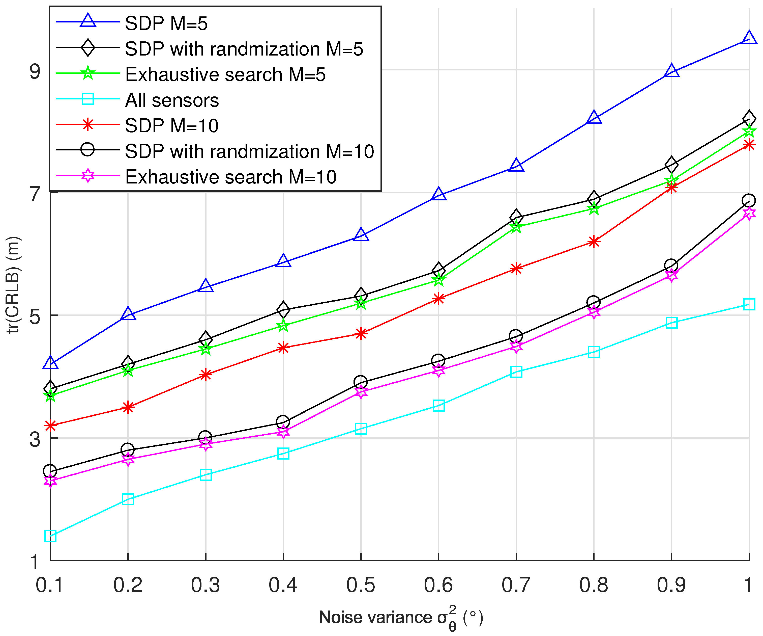
Figure 3 shows that the SDP with randomization method can obtain optimal estimation performance and close to the exhaustive search method when the number of selected sensors $M=5$ and $M=10$.

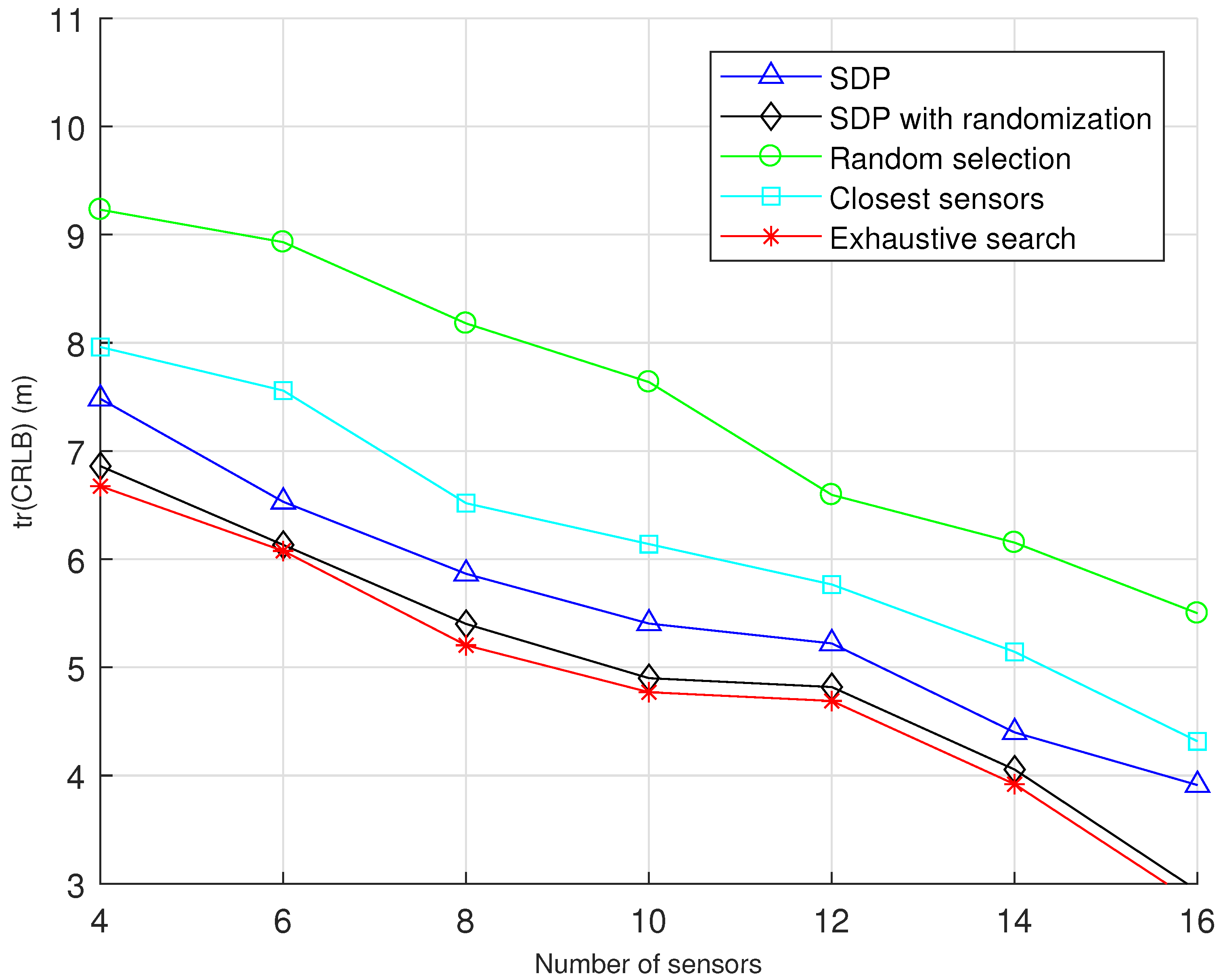
Figure 4 presents the $\mathrm{tr}\left(\mathrm{CRLB}\right)$ comparison of five different methods when the ${\sigma }_{{\theta }_1}^2\ne \cdots \ne {\sigma }_{{\theta }_N}^2\in \left[{0.1}^{\circ }\cdots ,1^{\circ }\right]$, ${\sigma }_{{\varphi }_1}^2\ne \cdots \ne {\sigma }_{{\varphi }_N}^2\in \left[{0.1}^{\circ }\cdots ,1^{\circ }\right]$. It is shown that the SDP with randomization always can obtain optimal estimation performance and is close to the exhaustive search method when the number of selected sensors is different. Besides, the $\mathrm{tr}\left(\mathrm{CRLB}\right)$ decreases with the increase of the number of selected sensors.

From the results, we can draw the conclusion that the SDP with randomization method has the optimal estimation performance when the noise measurements are identical or not.

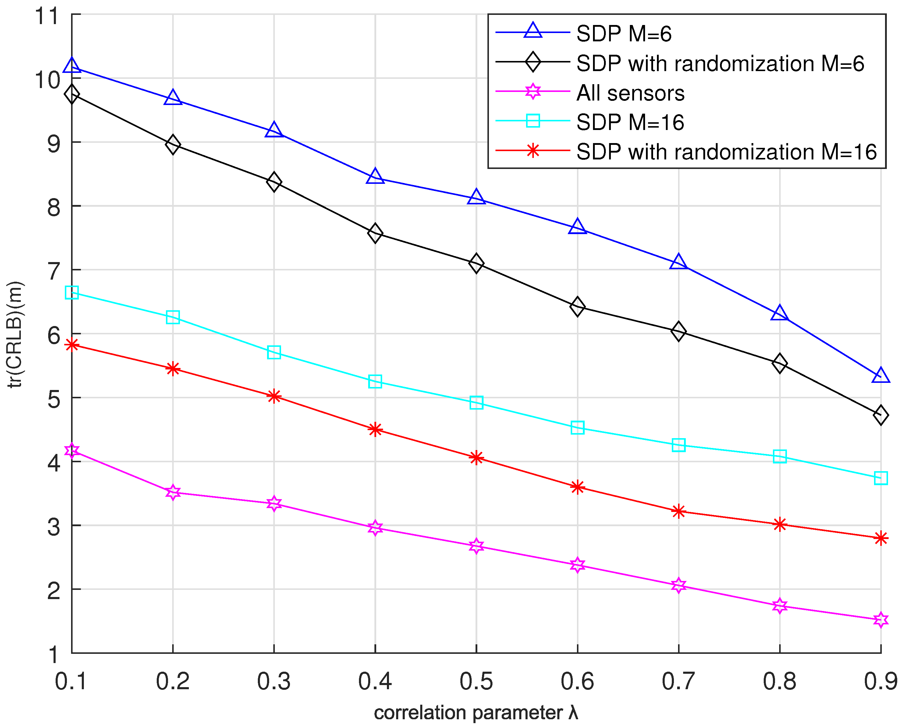
Then, we investigate the $\mathrm{tr}\left(\mathrm{CRLB}\right)$ when the correlation parameter ${\lambda }_{\theta }={\lambda }_{\varphi }=\lambda$ varies from 0.1 to 0.9, and the rest of the parameters are the same as Figure 1. Figure 5 presents the $\mathrm{tr}\left(\mathrm{CRLB}\right)$ comparison when $M=6$, $M=16$ and all sensors in the localization system. The $\mathrm{tr}\left(\mathrm{CRLB}\right)$ decreases with the increase of correlation parameter, which is consistent with the results in [25]. The noises can be reduced by subtracting one observation from the other due to the additive model with strongly correlated Gaussian noises, which can also obtain a better localization accuracy. Besides, the SDP with randomization method yields the optimal estimation performance.

6. Conclusions

In this paper, the sensor selection problem for the 3D AOA-based localization with correlated noises in UWSN is considered. The trace of CRLB is used as the objective function when the number of selected sensors is fixed. The sensor selection optimization problem is relaxing into a suboptimal semidefinite program using the convex relaxation, and then a randomization method is also adopted to improve the quality of the SDP solution. Furthermore, the proposed method has lower computational complexity than the exhaustive search method. Simulation results show that the performance of the proposed method gets better localization performance and approaches the exhaustive search method.

For future work, we will consider the case for multiple uncertain targets with the different correlated measurement noises, which changes the optimization problems to a convex combination of CRLBs. In addition, the sensor selection problem can also be developed for the uncertain moving target with the correlated measurement noise in the marine scenarios.