
Modelling of Powder Removal for Additive Manufacture Postprocessing


1
College of Engineering, Mathematics and Physical Sciences, University of Exeter, Harrison Building, North Park Road, Exeter EX4 4QF, UK
2
HiETA Technologies Ltd., Bristol and Bath Science Park, Dirac Crescent, Emersons Green, Bristol BS16 7FR, UK
*
Author to whom correspondence should be addressed.
J. Manuf. Mater. Process. 2021, 5(3), 86; https://doi.org/10.3390/jmmp5030086
Submission received: 28 June 2021
/
Revised: 30 July 2021
/
Accepted: 2 August 2021
/
Published: 6 August 2021
(This article belongs to the Special Issue Metal Additive Manufacturing and Its Post Processing Techniques)
Abstract
:A critical challenge underpinning the adoption of Additive Manufacture (AM) as a technology is the postprocessing of manufactured components. For Powder Bed Fusion (PBF), this can involve the removal of powder from the interior of the component, often by vibrating the component to fluidise the powder to encourage drainage. In this paper, we develop and validate a computational model of the flow of metal powder suitable for predicting powder removal from such AM components. The model is a continuum Eulerian multiphase model of the powder including models for the granular temperature; the effect of vibration can be included through appropriate wall boundaries for this granular temperature. We validate the individual sub-models appropriate for AM metal powders by comparison with in-house and literature experimental results, and then apply the full model to a more complex geometry typical of an AM Heat Exchanger. The model is shown to provide valuable and accurate results at a fraction of the computational cost of a particle-based model.
1. Introduction
Powder Bed Fusion (PBF) [1] methods are one of the main groups of Additive Manufacturing methods appropriate for metal forming. In these processes, successive layers of fine metal powder are layered on the manufacturing bed and fused together, for example using high-power lasers (Selective Laser Melting (SLM)) or Electron Beam Melting (EBM). This can produce high-resolution features including internal structures such as tubes and ducts, and challenging internal geometries which cannot be synthesised except through AM. A wide range of metal alloys are suitable for this sort of processing; in general, any metal that can be welded can be used for SLM. PBF can of course also be used for other materials as well, including polymers [2] and ceramics [3].
These methods, however, do present challenges as well, one of which is the removal of the surplus powder from the finished product. This will be particularly challenging when the product design includes interior structures such as fine tubes for compact heat exchangers or cooling ducts for gas turbine blades. In these cases, effective and complete powder removal is a requirement if the component is to function correctly, whilst at the same time redesign of the component to facilitate powder removal in postprocessing may not be desirable. Furthermore, the economic viability of producing large numbers of parts using powder bed systems depends heavily on the reduction in recurring costs [4], including in postprocessing. Finally, fine metal powders in powder bed systems can be costly, so waste should be avoided [5], and opportunities sought to maximise the recycling of otherwise wasted powder.
The surplus powder trapped inside the component can most conveniently be removed using vibrating systems [6]. Vibrating the component at high frequency or at the natural frequency of the component will fluidise the powder allowing it to flow out under gravity, similar to the process used for vibratory shake-outs in sand casting [7,8]. However, this process has rarely been analysed in any detail. It is particularly critical with the complex components now being developed such as compact heat exchangers, which may require a complex series of vibratory manipulations to fully remove all surplus powder and where any residual powder within the heat exchanger will substantially degrade performance. It is therefore essential to establish computational modelling techniques designed to predict powder flows for postprocessing in powder bed additive layer manufacturing.
1.1. Granular Flow
Flow of fluidised metal powders is a problem of granular flow. This is an important physical problem with a range of industrial applications, and so has been extensively studied in the past; it is thus appropriate to provide a short summary of some of the key aspects of granular flow at this point. The basic element of the physics involves particle-particle interaction, which can therefore be evaluated through Newton’s laws of motion; however, when the number of particles involved becomes very large, this may become unwieldy, in which case continuum mechanics approaches may be preferred. However, this is complicated by the fact that the individual particle-particle interactions may not be perfectly elastic. Whilst for fluid dynamics the Navier-Stokes equations can be derived as the continuum limit of the Boltzmann transport equation for molecular dynamics, for granular flow, due to the complexity of the physical interactions, there is no equivalent set of constitutive equations that can adequately represent the range of observed behaviour. Instead, empirical constitutive relations have been identified and used [9], particularly in engineering applications.
Empirically, there are various regimes which can be identified in granular flow [10,11], with differing constitutive relations:
- Quasi-static or granular solid or elastic-quasi-static. For a densely packed bed of particles sheared at a low rate, the stress is independent of the shear rate.
- Dense or granular liquid or elastic-inertial. Multiple and enduring contacts dominate, resulting in the stress being proportional to the shear rate.
The most important case in practice is that of dense granular flow. This is an observation from real-life, in the sense that hoppers, reasonably deep chute flows and commercial scale vibrated boxes all operate in a near packed state [13]. The particle flows in the current problem are certainly likely to be dense granular, with the additional simplifying factors that the particles have been industrially manufactured, and thus are likely to be reasonably uniform and spherical. However, if recycled powder is extensively used, the physical and mechanical properties may be significantly different and more complex [14].
1.2. Computational Modelling of Granular Flow
Computational work used to describe contact forces can be classified into the following categories [15].
- Microscopic models and particle-based simulations,
- Statistical mechanics and kinetic theories, and
- Continuum and phenomenological models.
As can be seen, this covers the full range of scales in the flow problem. Multiscale simulations [16,17] can combine several approaches such as Discrete Element Models (DEM) with Finite Element (FE) or Finite Volume (FV) continuum models in the same simulation. FE/FV methods can be employed to solve a macro-scale boundary value problem, while using DEM to generate the required non-linear material responses for each element. Such multiscale approaches can compliment traditional computational approaches in which the macroscopic models rely on internal variables pertaining to the granular texture, based on an understanding of the origins of the complex phenomenology of granular materials [18]. In both cases, continuum mechanics provides the framework for the computational analysis but the shift towards multiscale modeling has accelerated with increasing computational power. The question is how much of the microscale modelling is relevant to the macrobehavior [18], as well as how best to compute it.
For any given modelling challenge, there will be a balance between computational effort expended and fidelity, and the question here is: what level of fidelity is necessary to adequately represent the particle flow—in this case, the powder flow out of the component. To this end, molecular dynamics and continuum approaches are reviewed in the rest of this section.
1.2.1. Particle-Based Modelling
Particle-based models are based on the Lagrangian tracking of individual particles within the flow, and comprise both molecular dynamics models (MDM) and Discrete Element models (DEM); the main distinction between these being that MDM uses point particles whilst DEM considers finite size particles and includes the effects of shape and rotational degrees of freedom on their dynamics. As can be appreciated, these additional physical parameters can be of significant importance in assessing the behaviour of metal powders in PBF, and so DEM has frequently been applied to advance our understanding of the technique; see Section 1.3 for further details.
In implementation, these methods are usually either soft-particle methods or event-driven methods. Soft-particle methods are relatively slow and typically used for the analysis of dense flows for which the faster event-driven algorithms are not applicable [19]. Event-driven methods are typically faster for dilute rapid granular flows. However, they are impractical for dense flows in which collisions are very frequent and where the particles develop persistent contacts [19]. However, both methods are computationally costly when modelling very large numbers of particles.
1.2.2. Continuum Modelling
In parallel to the development of DEM for granular flow, the Computational Fluid Dynamics community has developed a range of techniques for dispersed multiphase flow modelling, which can be applied to high phase fraction flows with solid particles, appropriate for fluidised beds. These include Lagrangian particle tracking, in which the individual particles are tracked through the solution of Newton’s 2nd law for each particle (sometimes through coupling with a DEM code) or alternatively through the use of Eulerian–Eulerian (Eulerian Multiphase) modelling, where the dispersed secondary phase is modelled through a separate set of continuum mechanics equations.
The Lagrangian approach has some advantages for predicting particulate flows in which large particle accelerations occur and can also model flows involving polydispersed particle size distributions. An Eulerian–Eulerian approach is advantageous in flow cases where high particle concentrations occur and where the high void fraction of the flow becomes a dominant parameter of the flow [20].
The rheology for granular flows is only accurate for inertial numbers of less than around 0.3 [21,22], which limits its application to dense or liquid-like flows—in other words, gas-like behaviour at high inertial numbers cannot be modelled. For solid modelling in the rheology, the use of a simple Coulomb friction model for the flow threshold is also a limitation and the complex transition between solid-like and liquid-like behaviour is ignored, such as shear bands, intermittent flows and hysteresis [23].
Eulerian-Eulerian models for gas-particle flows are practical for industrial systems as they balance CPU cost with simulation accuracy [24]. In many industrially relevant cases, there are regions in the flow domain where kinetic stresses dominate, other regions where frictional stresses dominate, and also regions where the two effects are similar in magnitude. Thus, it is important to develop rheological models that include both contributions [25].
Often DEM and continuum FE can be applied to similar systems and gain equivalent results, such as for a particle hopper (conical hopper simulated with FEA [26], flat bottom hopper simulated with DEM [27]). Direct comparisons, where they have been performed, show the hardly surprising result that whilst DEM can more detailed [28], FEA is computationally much less costly [29], taking only hours to compute as against days for DEM.
1.3. Powder Flow Modelling for AM
DEM has seen extensive application in modelling aspects of the PBF AM process, but principally has been applied to the manufacturing process itself, particularly the deposition of the particle layer and the melt process. Various papers in the literature investigate the spreading process, particle packing, or the melting and fusion, or attempt to integrate all three areas.
Bed preparation typically involves either rollers or the use of a blade to level the bed. Chen et al. [30] use DEM to investigate the flow of powder layered by a blade, comparing with video recordings of the process for validation. A recent study [31] investigated the packing fraction and its variation with gap thickness and blade velocity for the deposition of a thin powder layer representative of a titanium alloy AM powder. Haeri et al. [32] used DEM to model the spreading of non-spherical particles as a compact layer for sintering. They used Scanning Electron Microscopy to characterise the shapes of particles of commercial and custom-milled PEK/PEEK polymer composites, which were then represented in the DEM code (LAMMPS [33]) using composite particles built from the basic spheres. This enabled them to examine the relationship between particle shape, spreading (via roller or blade) and properties of the resulting bed.
Spreading using rollers has also been investigated using continuum mechanics methods. As discussed above, this requires the development of appropriate constitutive relations. Suitable equations have been developed [34] and applied in FE [35] and mathematically [36]. As is recognised, such methods cannot easily incorporate particle shape information in the way that DEM can, but the simulation cost is significantly lower than full DEM. We also recognise that whilst the particle shape is highly relevant for particle packing, it may be less so when the particles are fluidised, as is the case for our application. A radically different approach to the spreading is used by Desai and Higgs [37], who use back propagation Neural Networks trained on a combination of experimental and physics-based (in-house DEM) modelling of particle spreading to predict spread layer properties such as mass of material, layer roughness and porosity.
DEM can also be used to model heat transfer between particles, and so has found a use in modelling the sintering process, incorporating suitable particle-particle interactions to model the fusion [38,39,40]. Wei et al. [41] review mechanistic models for metal based AM, principally concentrating on the thermal and hydrodynamic aspects of the melt pool created by the local melting, but do cover some aspects of powder packing models used to calculate aspects of the initial layering process.
Steuben et al. [42] present the modelling and design of an in-house DEM-based multiphysics code capable of simulating the particle deposition and sintering process for complete components; the simulation of the construction of a turbine blade is demonstrated. Performance benchmarking with the well known DEM package LIGGGHTS [43] is also presented. Lee and collaborators [44] use the LIGGGHTS package to simulate the whole PBF process, with a simplified powder deposition process, recoating, laser heating and holding process. They also validate the basic DEM modelling using the experimental case of metal particles draining from a hopper.
Another area in which metal particles are being processed for AM is for direct energy deposition methods such as coaxial laser metal deposition. In [45] the commercial CFD code CFD-ACE+ is used to model the gas-propelled flow of metal powder before and after leaving the nozzle. In this work, the gas flow is simulated using continuum mechanics (Finite Volume CFD) and then Lagrangian particle tracking utilised to track the particle behaviour in the gas stream. Similar methodology was used in [46], who compare experimental data for different nozzles, and in [47].
1.4. Overview and Structure of This Paper
In contrast to the work analysed in Section 1.3 above, our primary interest here is in the powder removal from the interior structure of a (largely) finished AM component. Modelling this requires the computational modelling of a range of granular physics, including energisation from the wall motion during part vibration and the resulting flow of the fluidised medium. The work presented in this paper details the development of an Eulerian multiphase model for metal particles characteristic of AM use and its validation against experimental data taken from the literature. The rationale behind the choice of a continuum mechanics approach here over the more detailed DEM models was to do with relative computational cost, particularly when applied to geometrically highly complex problems; DEM is unlikely to be a practical choice for simulating powder drainage from complex components.
The structure of this paper is as follows. In the next section (Section 2), we develop the mathematical equations used to model the powder flow and discuss their solution using the open source Computational Continuum Mechanics (CCM) tool OpenFOAM. Section 3 presents the details of the particular sub-models specifically developed to handle this type of granular metal powder flow, and their validation against experimental data from the literature. Section 4 presents the results of the full simulation model applied to a complex geometry representative of a true life case (based on the Morimoto duct geometry [48]). The results are reviewed and our major conclusions are presented in the Conclusions section (Section 5).
2. System of Equations
2.1. Solver Development
In this work, a two-fluid model of fluidised AM metal powder is developed based on the OpenFOAM Computational Fluid Dynamics (CFD) open source toolkit. Specifically, this was based on the OpenFOAM solver twoPhaseEulerFoam, which uses a continuum or the Eulerian-Eulerian approach, in which the motion of the bed is considered as the motion of two interacting continua representing the air and the powder as described in Section 1.2.2. A frictional-kinetic theory is used in order to model the powder as a solid and gas. The Eulerian–Eulerian approach models particles and air using the following sub-models:
- Drag coefficient,
- Granular viscosity (collisional, kinetic and frictional terms),
- Granular pressure (collisional and kinetic terms),
- Granular conductivity (collisional and kinetic terms),
- Radial distribution function,
- Particle bulk density,
- Production of granular energy by particle-particle collision, and
- Production and dissipation of granular energy by gas-particle slip.
The drag coefficient implies that there is inter-phase momentum transfer. The rest are sub-models used to synthesize the conservation equations with the kinetic theory for granular flows. As such, some of them contain terms representing particle collision, kinetic and frictional behaviour. To complete the solver, we have provided existing or new sub-models for these physical mechanisms, and where these are new we have to validate the new modelling.
2.2. Governing Equations
In an Eulerian dispersed multiphase model, we introduce the phase volume fraction as the ratio of the volume of phase i in the cell divided by the total volume of the cell V.
and obviously . The continuity and momentum equations for the dispersed phase are given by Equations (2) and (3).
where , and are the velocity, density and pressure of the i-th phase ( for the solid particulate phase and for the gas/continuum (air) phase). is the (predominantly viscous) stress, and represents the interchange of momentum between the phases due to processes such as drag. In a similar manner, the conservation equations for the continuous phase are given by Equations (4) and (5).
The kinetic theory of granular flow introduces the concept of granular temperature () to have closure with the conservation equations [49,50]. Therefore, the properties of the dispersed phase are functions of this granular temperature, which is determined by solving the granular energy transport equation, given by Equation (6).
2.3. Sub Models
Both the dispersed phase and the continuous phase are treated as Newtonian fluids and the stress tensors are given by Equations (7) and (8).
The particle bulk density is given by Equation (9).
The dissipation of granular energy by particle–particle collision is given by Equation (10).
The production and dissipation of granular energy by gas-particle slip is given by Equation (11) from Louge.
Since the dispersed phase has relatively small particles and a large density, the interphase drag force dominates over the other forces such as lift and virtual mass. Therefore, the coefficient has just a drag contribution. The Gidaspow-Ergun-Wen-Yudrag model is suitable for both dense and dilute flows. The Ergun model is based on fixed liquid-solid beds at packed conditions () given by Equation (12). The Wen-Yu model is based on settling experiments of solid particles in liquid and is suitable for dilute flows () as shown by Equation (13).
The solid stress tensor includes contributions from both bulk and shear terms arising from particle momentum exchange due to translation and collision. A frictional component can also be included to account for the effect of the viscous-plastic transition when the maximum solids volume fraction is reached, as shown by Equation (16).
The kinetic viscosity model developed by Gidaspow is given by Equation (17).
The collisional viscosity model by Gidaspow is given by Equation (18).
When the solid volume fraction exceeds a critical value , the solid viscosity given by Equation (20) is added to the viscosities calculated from Equations (17) and (18) and limited beyond .
The conductivity model developed by Gidaspow is given by Equation (21).
The granular pressure, is given by the Lun model, as shown in Equation (22). Physically, it refers to a pressure which is created due to the movement of particles due to shear and also due to particle–particle collisions.
The radial distribution function used is by Sinclair–Jackson. It is a continuous function and begins at zero and asymptotes to a maximum near the maximum volume fraction . It can be seen as a measure of the probability of inter-particle contact [51].
3. Sub-Models: Development and Validation
The mathematical models outlined in Section 2 above are by and large generic and applicable to a range of multiphase flows. For the specific problem of powder removal flow in AM, there is a range of specific physics which has to be modelled, and for which we have to develop and validate specific models. In this section we explain these specific models we have developed here and how they have been validated against experimental data from the literature. This includes modelling cohesive forces relevant for aluminium powders and the effect of wall vibration. We will discuss these aspects and the experimental validation in the following section.
3.1. Cohesive Forces
There are several classifications of powder that characterise the relevant forces that need to be modelled [52]. In class A (Aeratable) powders, cohesive forces can be influential, whereas in class B (Bubbling) powders, gravity dominates over cohesive forces. Class C (Cohesive) are powders where cohesion dominates and class D (Dense) lists powders confined to large or very dense particles. The classification is determined using a sub-divided chart based on the density difference between the solid and fluid phase and the mean particle size [52]. The chart has density difference on the y-axis and mean particle size on the x-axis. In the work reported here, two powders have been selected which are relevant to additive layer manufacturing, as follows:
- Inconel 625—, → Geldart Type B powder (cohesive force weaker than gravity);
- AlSi10Mg—, → Geldart Type A powder (cohesive force as important as gravity).
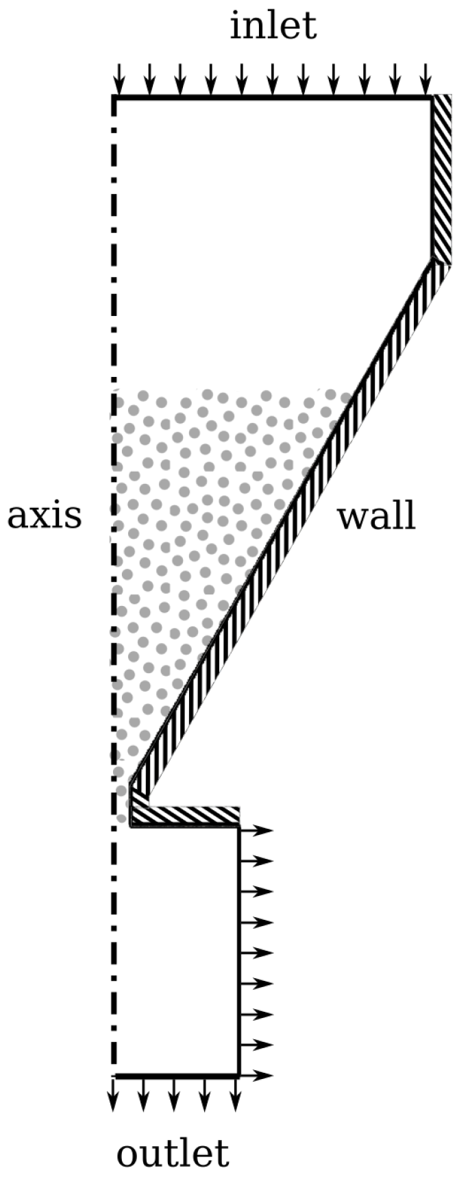
Experimental data are available in the form of the Hallflow test, in which the time taken for a measured mass of powder to drain from a conical hopper. Figure 1 shows the boundary conditions and geometry for the Hallflow test case. The model is axi-symmetric with a segment angle of bound between cyclic boundaries. The inlet radius is mm, whilst the outlet radius is mm. The domain has a total height of mm, and the wall is at an angle of to the vertical. The orifice radius is mm and the length is mm. The inlet and outlet boundary conditions are atmospheric, whilst the wall boundary condition is the Johnson-Jackson condition for granular flows with a specularity coefficient of . Experimental tests carried out in accordance to the correct ASTM standard [53] were made available by the powder manufacturer for the two powders being examined so that it can be compared with the results of the Eulerian-Eulerian simulations. In the CFD simulation, the mass flow rate can be derived from the phase fraction as follows:
3.1.1. Modelling Cohesive Forces
Cohesive forces are weak compared to gravitational forces for the type B Inconel powder, so no cohesion model was used for this validation. Conversely, for the type A aluminium powder, cohesive forces are important. Various cohesion models have been proposed in the literature including a model based on a cohesive pressure [54] and agglomerate diameter [55]. However, the simplest model that gave sensible results used a cohesive pressure combined with a cohesive viscosity [56]. This is based on the idea of adding a pressure term to represent cohesion, as stated and validated by other researchers [54].
Cohesion is added as an additional granular pressure and viscosity. Equation (25) is the cohesive pressure and Equation (26) shows the cohesive viscosity.
in Equation (25) is a factor used due to the uncertainty about the exact value of , the inter-particle cohesion force. With the aluminium powder (type A) it is assumed that Van der Waals forces are the primary source of cohesion, but there is still uncertainty over the value of in the model [57]. In order to calibrate the value, the Hallflow test is utilised with data supplied by the powder manufacturer.The velocity is given by Equation (27)
3.1.2. Results—The Hallflow Test
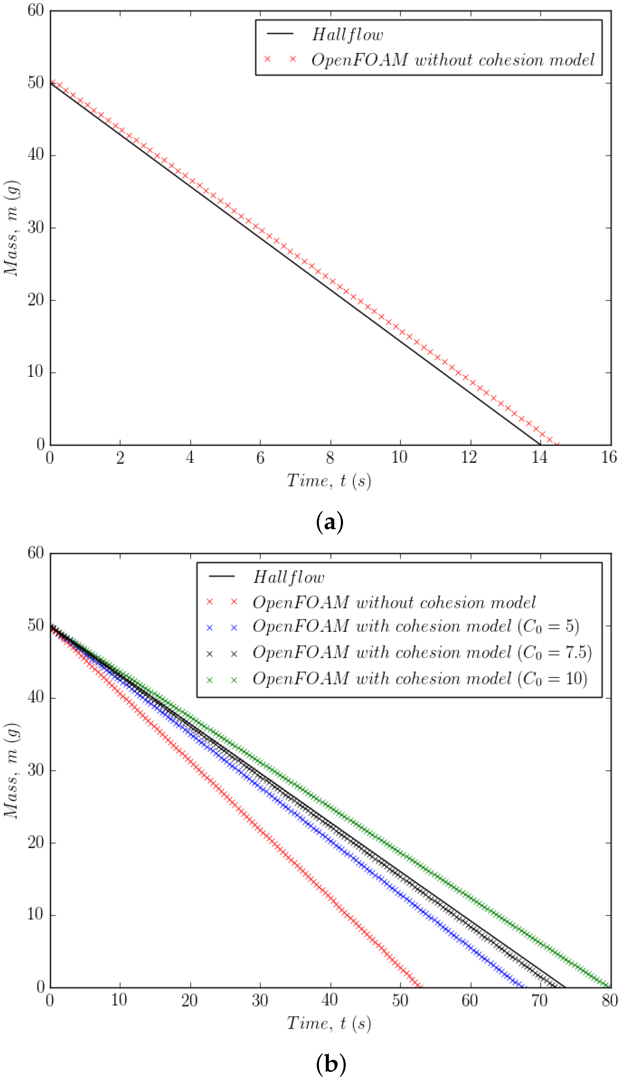
Since cohesive forces are weak compared to gravitational forces for the type B Inconel powder, no cohesion model was used for this validation. Figure 2a. shows that the model predicts a linear variation in the mass over time. For the experimental data, only the initial mass and the time to empty were available and so we have had to assume a constant value for the flow rate. However, it is reasonable to assume this, as shown in experiments by measuring the mass over time [58]. In detail, the emptying process consists of an initial transient as the flow process starts, followed by a pseudo-steady state period when the flow is established during which the hopper empties, finishing with a final transient as the remaining powder drains away. The pseudo-steady state period represents almost all of the emptying process. The flow rate during this period is constant and it is this region that is used for measuring the mass flow rate. The difference for the time to empty for g of powder between the Hallflow data and the CFD model is less than and the mass flow rate is less than different.
With the aluminium powder (type A) where Van der Waals forces are the primary source of cohesion, we need to calibrate the value of . Figure 2b. shows that the cohesion model improves the comparison with the Hallflow data, and it is clear from this that the cohesion model has a significant influence on the solid volume fraction, due to the addition of the cohesive pressure and viscosity. Thus the choice of the factor needs to be optimised to produce the correct mass flow rate. The time to empty is within of the Hallflow test using a cohesion factor of . However, it is unlikely that this cohesion model can be used in case of vibrating walls, as the breakup of agglomerates by the dominance of vibrational energy over collisional and cohesive energy is not being considered. For this reason, the model is limited to Hallflow data where vibration is not being used to fluidize the powder.
3.2. Wall Vibration
In order to simulate wall-normal vibration, it was necessary to develop a new boundary condition. Several approaches were considered, including a sinusoidal gravity term [59], mesh motion, finite element coupling and use of the granular temperature [60]. The frequency of vibration (on the order of kHz) is likely to be far too high to utilise mesh motion and finite element coupling, due to the computational overhead of simulating the individual wall motions involved. On the other hand, a sinusoidal gravity term is simplest, but only allows for vibration to be applied in the direction of the gravity vector. The reality of the vibration applied to remove the powder is that it is wall-normal. Therefore the most efficient method, which also provided physical realism, was to utilise the fact that the kinetic theory of granular flows requires a pseudo-heat flux at the wall, which can be used to simulate wall-normal vibration. The equation for wall vibration was developed by Richman [60], by considering that random vibrations occur in all three perpendicular directions. Here it is assumed that in-plane vibration components do not contribute to the energy transfer such that only wall-normal vibration is considered. The form used here was given by Viswanathan [61]:
For comparison purposes, the validation case also includes a model using a gravity term representing the vibration. The equation for this simply modifies the global body force of gravity in the momentum equation for the air and particle phases [59]:
3.2.1. Wall-Normal Vibration Test Case
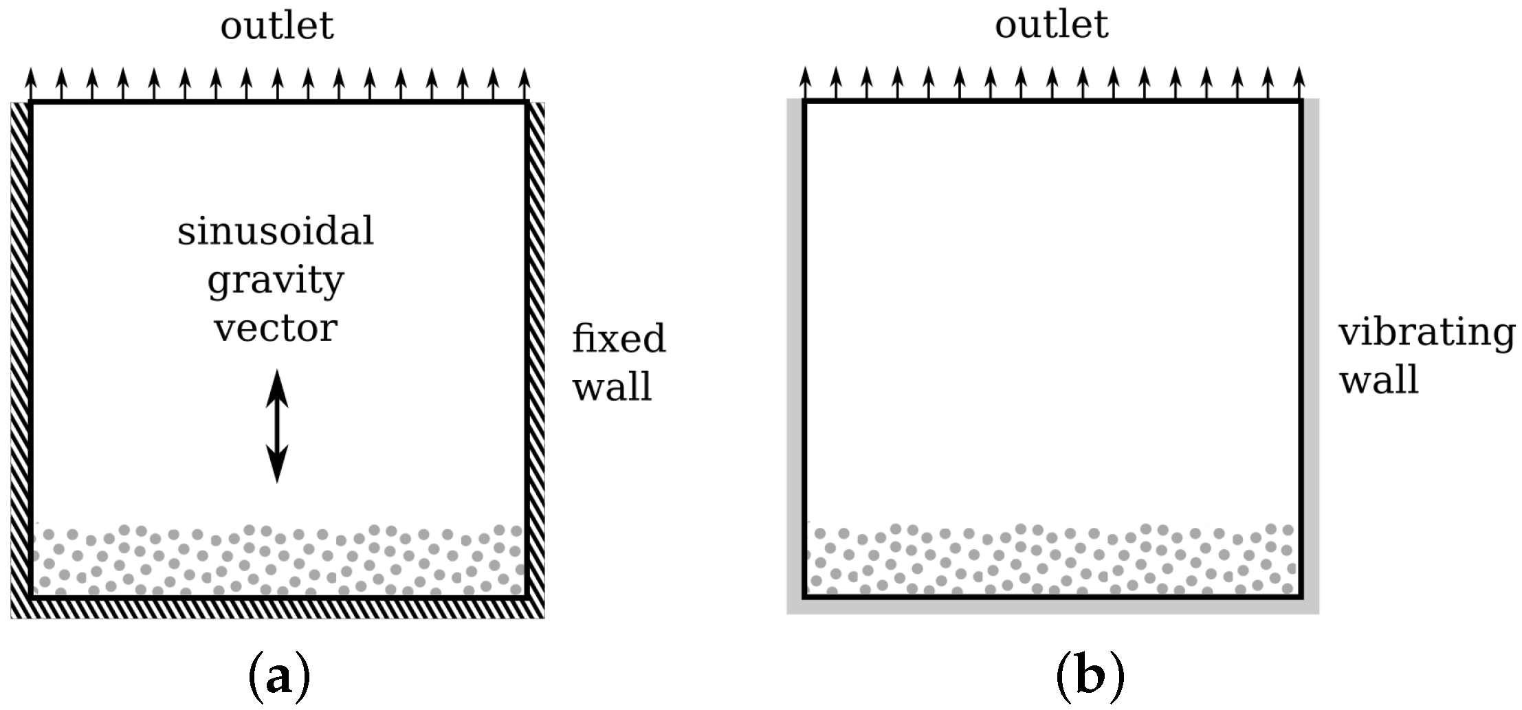
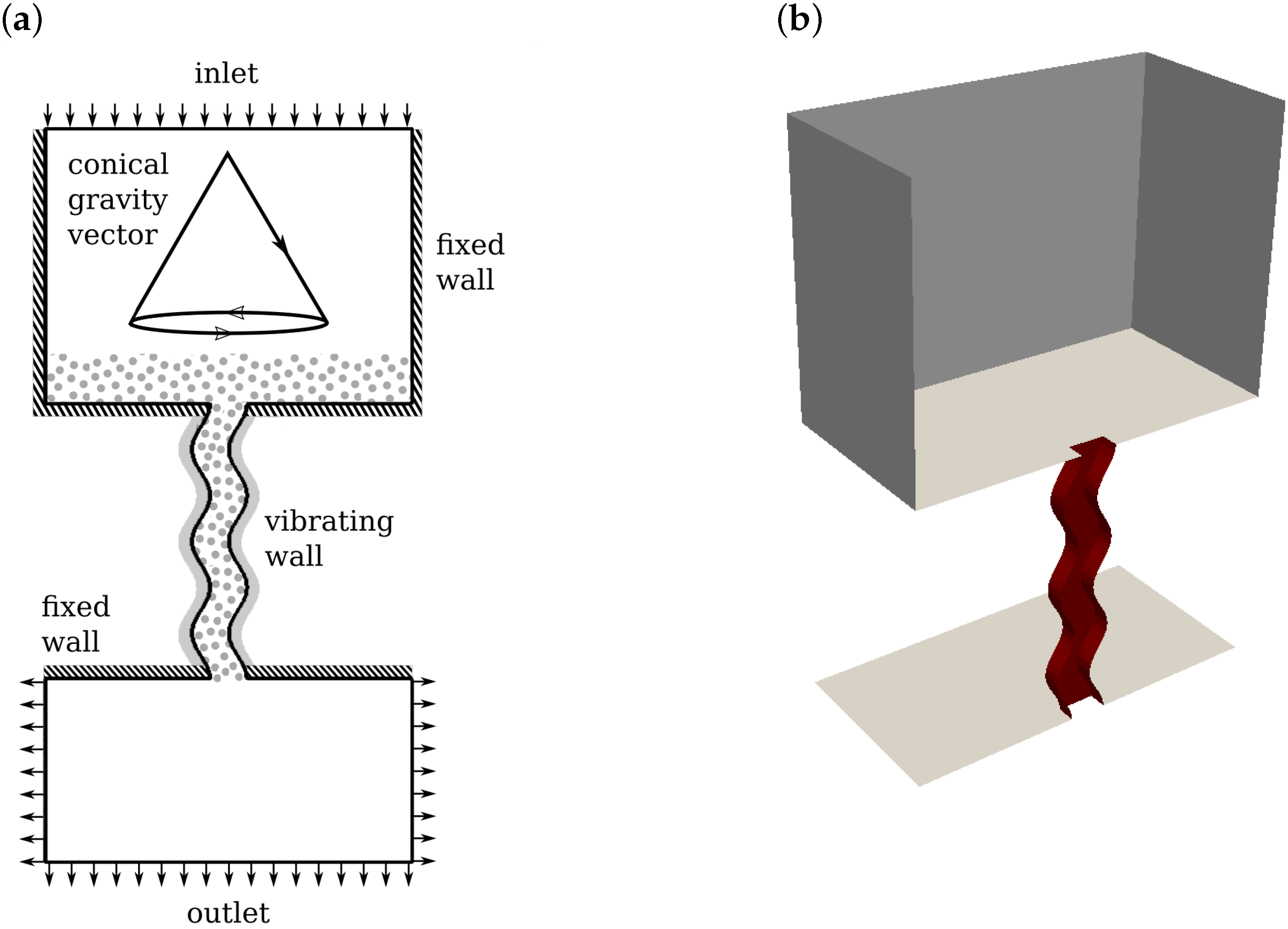
Validation of the vibration modelling was carried out using a vibrofluidisation case for which experimental data (using large dolomite and fine glass particles) are available [62]. Figure 3 shows the boundary conditions for the two models analysed in this section. The domain is 2D with a width and height of mm, and a depth of mm. The domain is initially filled with particles to a height of mm or mm depending on the test case. The boundary condition at the outlet is an atmospheric pressure boundary. The wall boundaries can either be fixed or vibrating. If fixed, then a sinusoidal gravity vector is imposed in the vertical plane. If vibrating, the frequency can vary between Hz and Hz according to the validation case data, whilst the amplitude is fixed at mm.
3.2.2. Effect of Vibration on Solid Volume Fraction Field
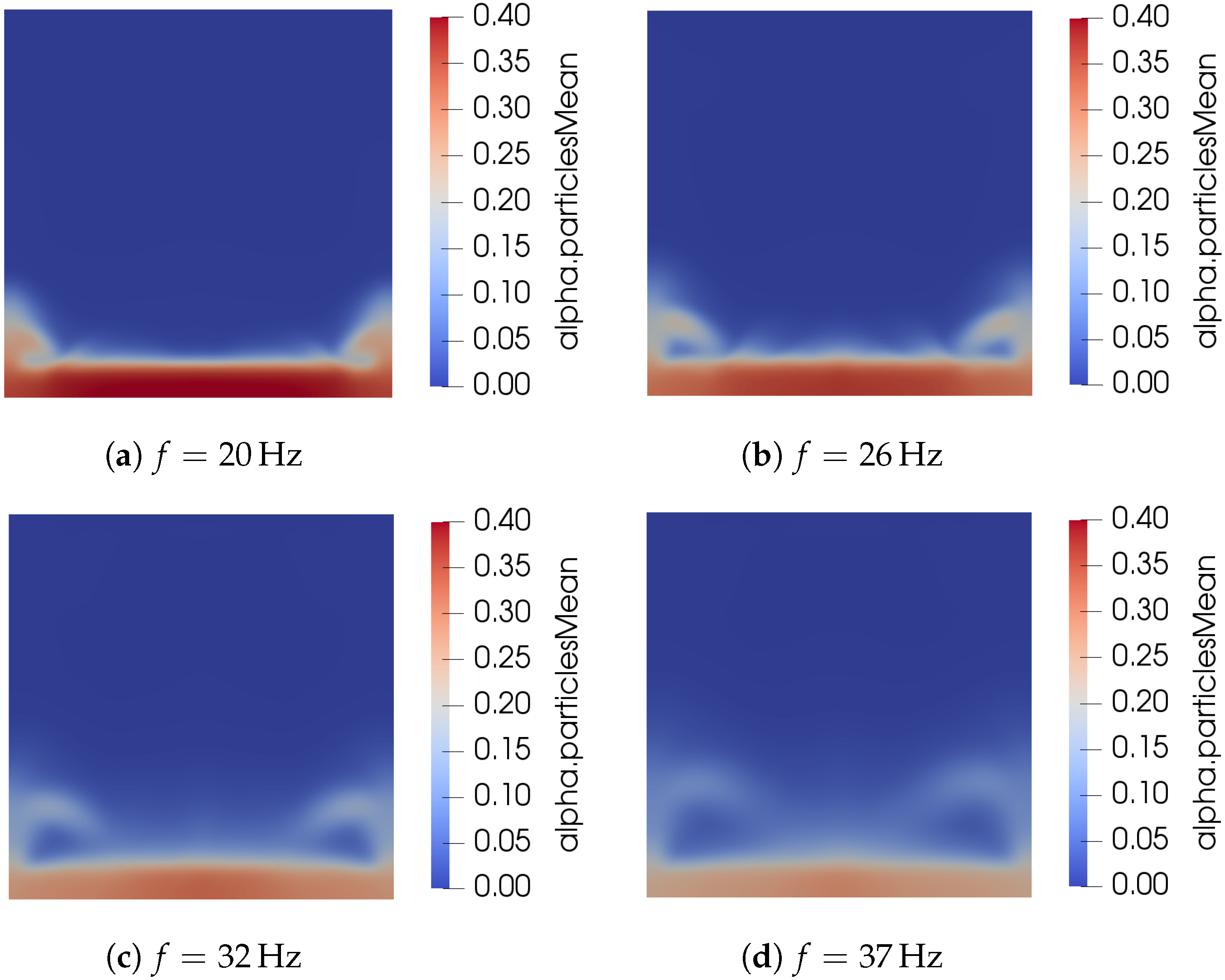
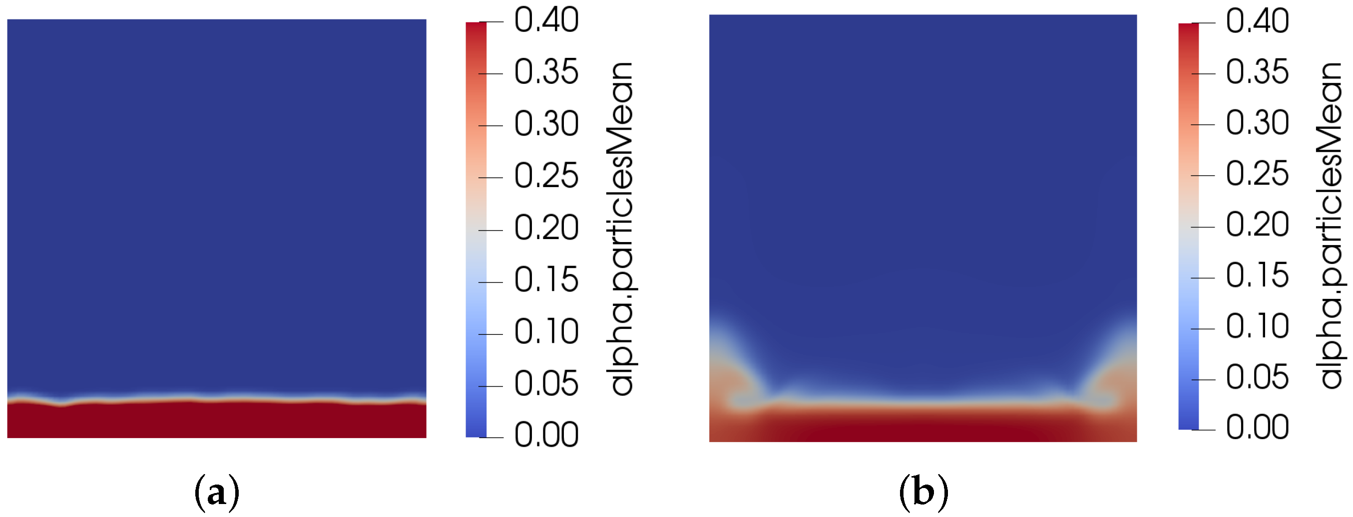
Figure 4 shows the volume fraction field as computed by considering that the wall boundary condition is given by the pseudo-heat flux in Equation (28). It is clear that increasing the frequency of vibration dilutes the volume fraction field and increases the height of the splashes seen near the corners.
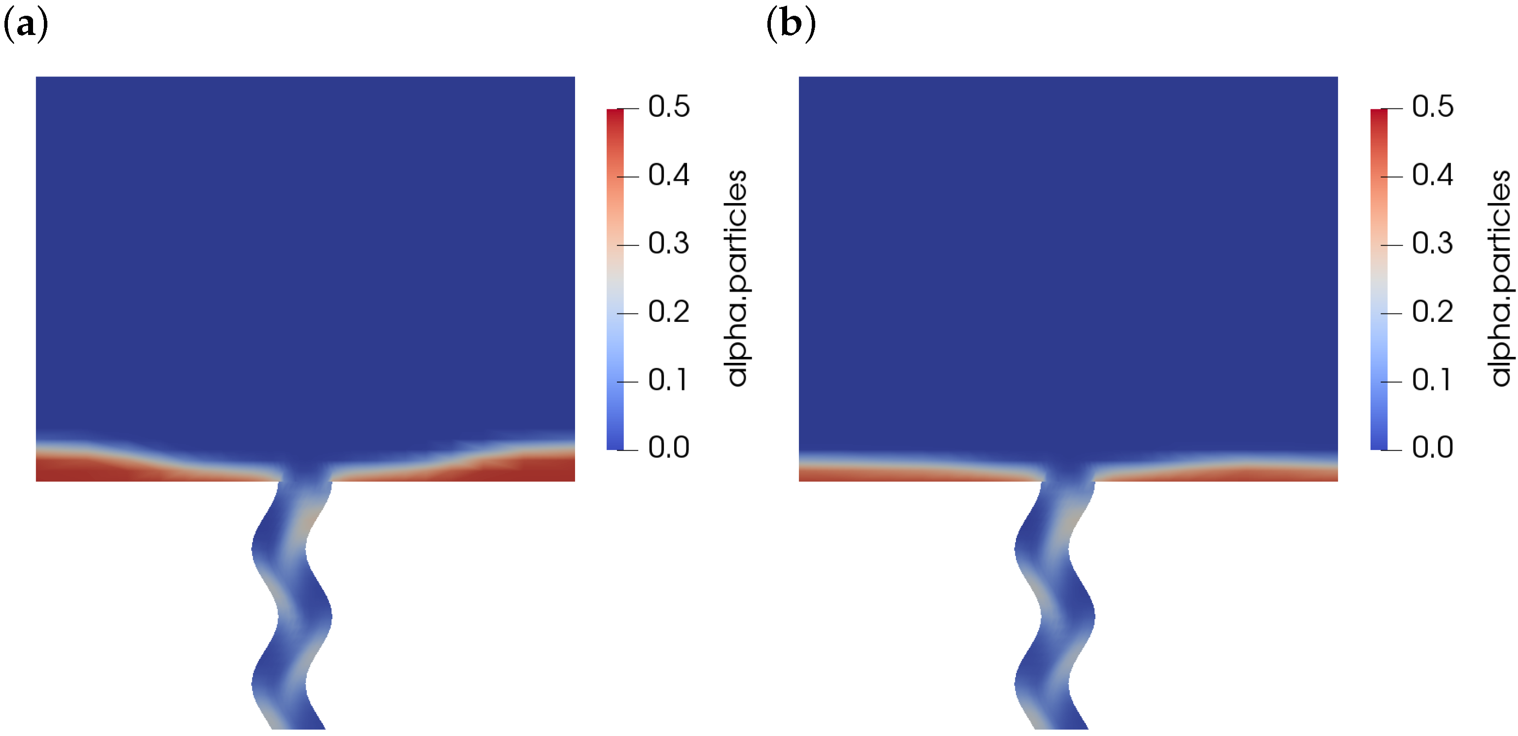
Figure 5 compares the result of assuming the gravity body force can represent vibration using Equation (31) with Equation (28) using the pseudo-heat flux approach. The gravity body force approach cannot capture the splashes seen at the corners, because vibration is only implemented in the vertical direction of gravity.
3.2.3. Effect of Vibration on Surface Height
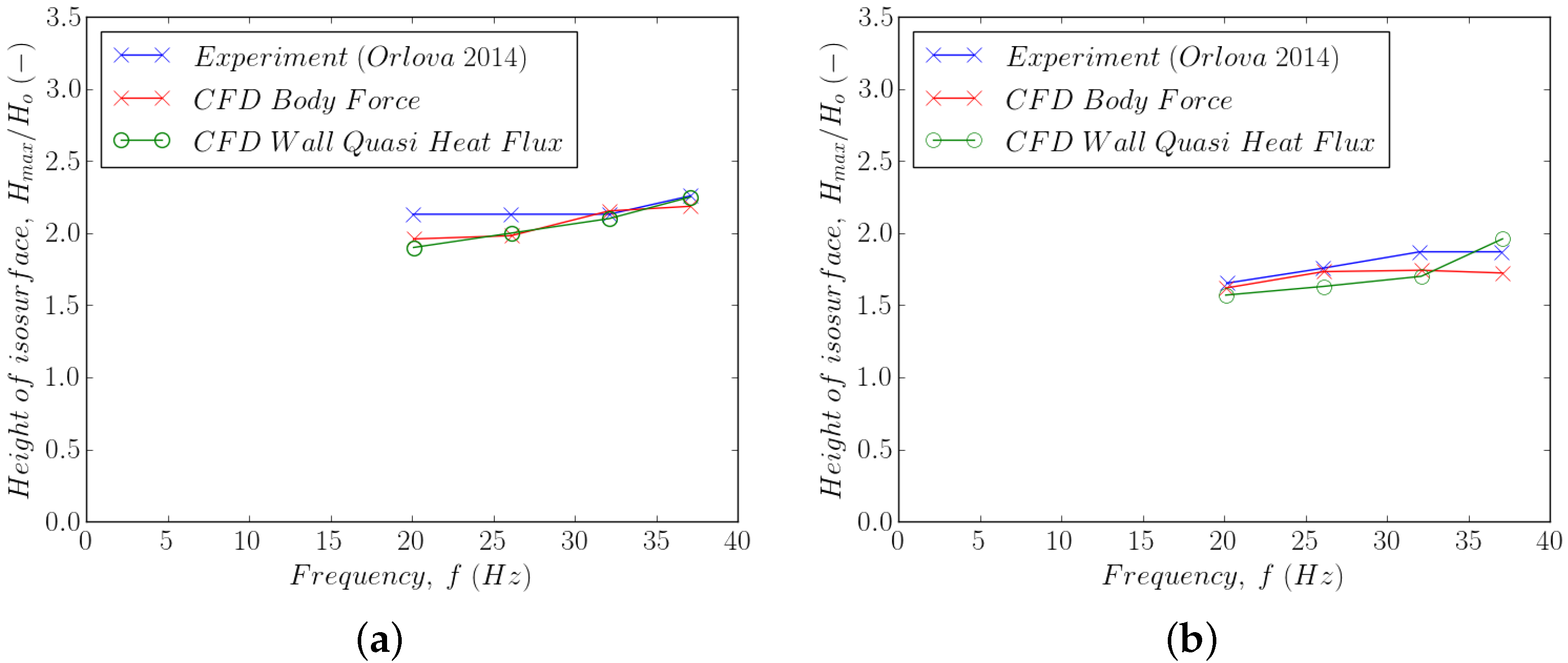
Quantitative validation of the new boundary conditions was sought using the height of the volume fraction field as an isosurface at a value of . These measurements are shown in Figure 6 via a comparison between experimental measurements [62], the pseudo-heat flux approach of Equation (28) and the gravity body force approach of Equation (31). The results show that the difference is less than and the trend is broadly similar.
3.2.4. Effect on Granular Temperature
The previous friction model (Equation (20)) applied to a case where wall-normal vibration was not used. In cases where the particles are relatively large ( mm) and the vibrational frequency is low (< Hz), as in the experiments used above, this is still a reasonable assumption [59]. For cases where and higher-frequency vibration, the vibration may well affect the frictional viscosity. To account for these cases, the model of Srivastava-Sunderesan is used. This was verified by comparison with the test case of Srivastava-Sunderesan (which differs by its use of alternative sub-models). This differs from the usual form of the Schaeffer frictional stress, as it includes a term that allows strain rate fluctuations (represented by granular temperature) . Based on this, Equation (20) can be modified:
4. Modelling of a Complex Duct
The objective of the work reported in this paper is to provide a model for the powder drainage from arbitrarily complex internal ducting manufactured through AM. Having developed such a model and validated the main new models (Section 3), we are now in a position to apply this to a more complex geometry. The geometry used for this is derived from the geometry proposed by Morimoto [48,63], developed as an optimal shape design for a recuperator heat exchanger. The design uses oblique wavy walls to optimise heat exchange between separated flows of hot and cold fluid, and has been designed for use in compact heat exchangers. As such this is characteristic of the types of AM components we are interested in [64].
4.1. Test Case Description
Figure 7 shows the boundary conditions for the Morimoto test case. The duct has three wavelengths with an amplitude of mm and wavelength of mm with a wall separation of mm in both orthogonal directions. This duct was fed from a square-cornered hopper. The reason for this was to make the mass versus time profile non-linear by allowing powder to become trapped in the corners. This also provided the opportunity to investigate the effect of further manipulation of the unit, in particular the effect of tilting the unit to remove powder from the corners. The hopper has a width and depth of mm, with a height of mm, the outlet has a width and depth of mm and a height of mm. The hopper is initially filled with a mass of powder of g, a value chosen to minimise the time required to empty the vessel whilst still allowing linear and non-linear regions of the flow regime to be observed. The inlet and outlet boundary conditions are set to atmospheric pressure.
In each of the following cases, the effects of manipulation, vibration and the effect of both together are studied. The effect of unit manipulation is simulated by allowing the direction of the gravity vector to precess around a cone of half angle ( ranging from to ) by defining it as
where
with a rotational speed . This appears as an additional body force in the momentum equation for both the particle phase and the air phase. It also introduces a centrifugal acceleration of form
This appears as a source term on the right hand side of the momentum equation for the particle phase [65]. It is assumed that the air phase is unaffected by centrifugal forces due to its relatively low density. The effect of vibration is introduced by use of the pseudo-heat flux given by Equation (28), which is introduced as a new boundary condition into the code. The vibrating walls use this pseudo-heat flux condition with a frequency of Hz and an amplitude of mm and a specularity coefficient of 1 unless otherwise specified. It was found that application of the wall-normal vibration to all walls resulted in powder being driven against gravity in the hopper. This meant that it could no longer supply the Morimoto geometry with powder. Instead, the vibration was applied only to the Morimoto section as shown in Figure 7. The fixed walls use the Johnson–Jackson boundary conditions for partial slip with a specularity coefficient of . Equation (24) was used to measure the mass flow over time.
In all, four different wall separations were investigated; mm, mm, mm and mm. The CPU time for this geometry varied with the wall separation from 21 h 44 min for mm to 2 h 14 min for mm. This is largely due to the time taken to empty the device, as the number of cells varied from 63,756 for mm to 150,108 for mm, whilst the time to empty varied from s for mm to s for mm. This was measured on a 12 processor run, on Intel Xeon processors at GHz, with 35 MB cache.
4.2. Effect of Manipulation/Vibration
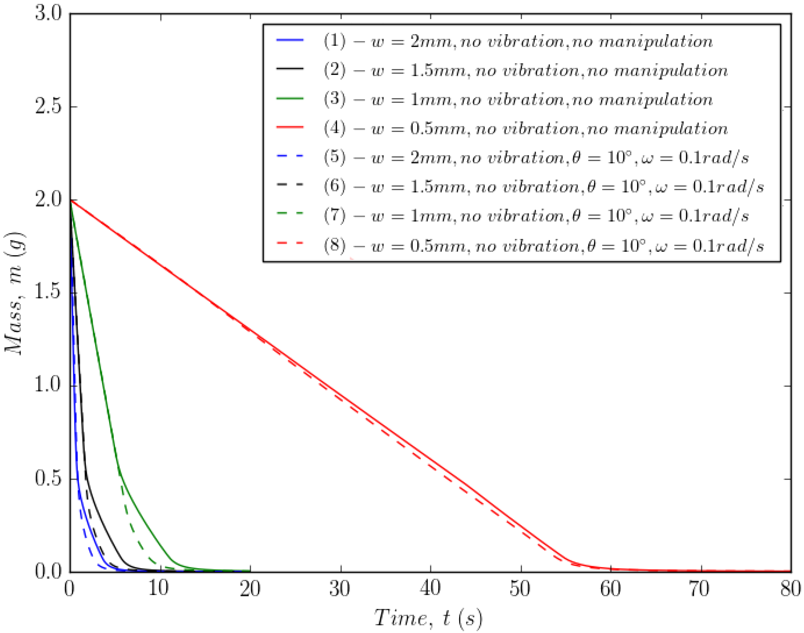
The effect of manipulation (moving the unit bodily around) with or without wall vibration (i.e., shaking the unit) is examined in this section. The basic effect of the manipulation is shown in Figure 8 which contrasts the powder remaining in the hopper at s (i.e., almost empty) for a stationary geometry (Figure 8a) with that for a rotational manipulation , . As can be seen, the tilting manipulation has clearly encouraged more of the powder to drain out of the unit which would otherwise become trapped in the corners of the hopper. Figure 9 demonstrates the drainage of the powder over time for various wall separations w. The effect of the corners of the square hopper is to slow the powder emptying in the final stages (solid lines for the different duct geometries), whilst the manipulation sequence clearly reduces this effect (dashed lines).
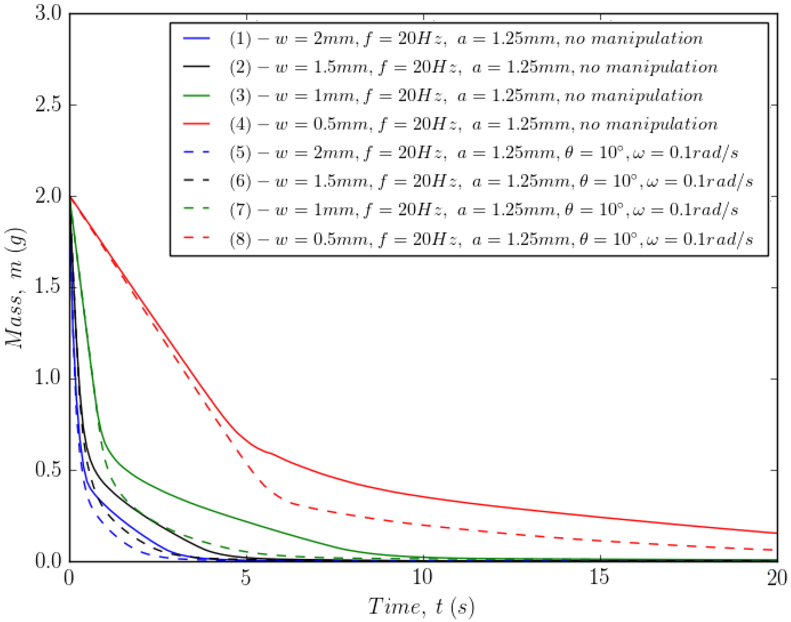
We can contrast this with Figure 10 and Figure 11, which show the combined effect of manipulation and vibration on the emptying. Figure 10 shows that the combination influences the final transient of the emptying process. This suggests that the best combination is to use the energisation of wall-normal vibration together with manipulation. Figure 11 demonstrates that the manipulation sequence with vibration has a similar effect to that shown in Figure 8, since powder can be more effectively removed from the corners with manipulation. This feeds the subsequent energisation of the powder by vibration in the Morimoto section.
Two measures were used in order to quantify the previous figures, the maximum mass flow and the time to empty. The maximum mass flow was taken during the pseudo-steady state region () by taking the steady gradient of the mass versus time profile as shown in Equation (38). The time to empty was taken when the mass fell to of the original mass ( g and g) and was determined using linear interpolation as shown in Equation (39).
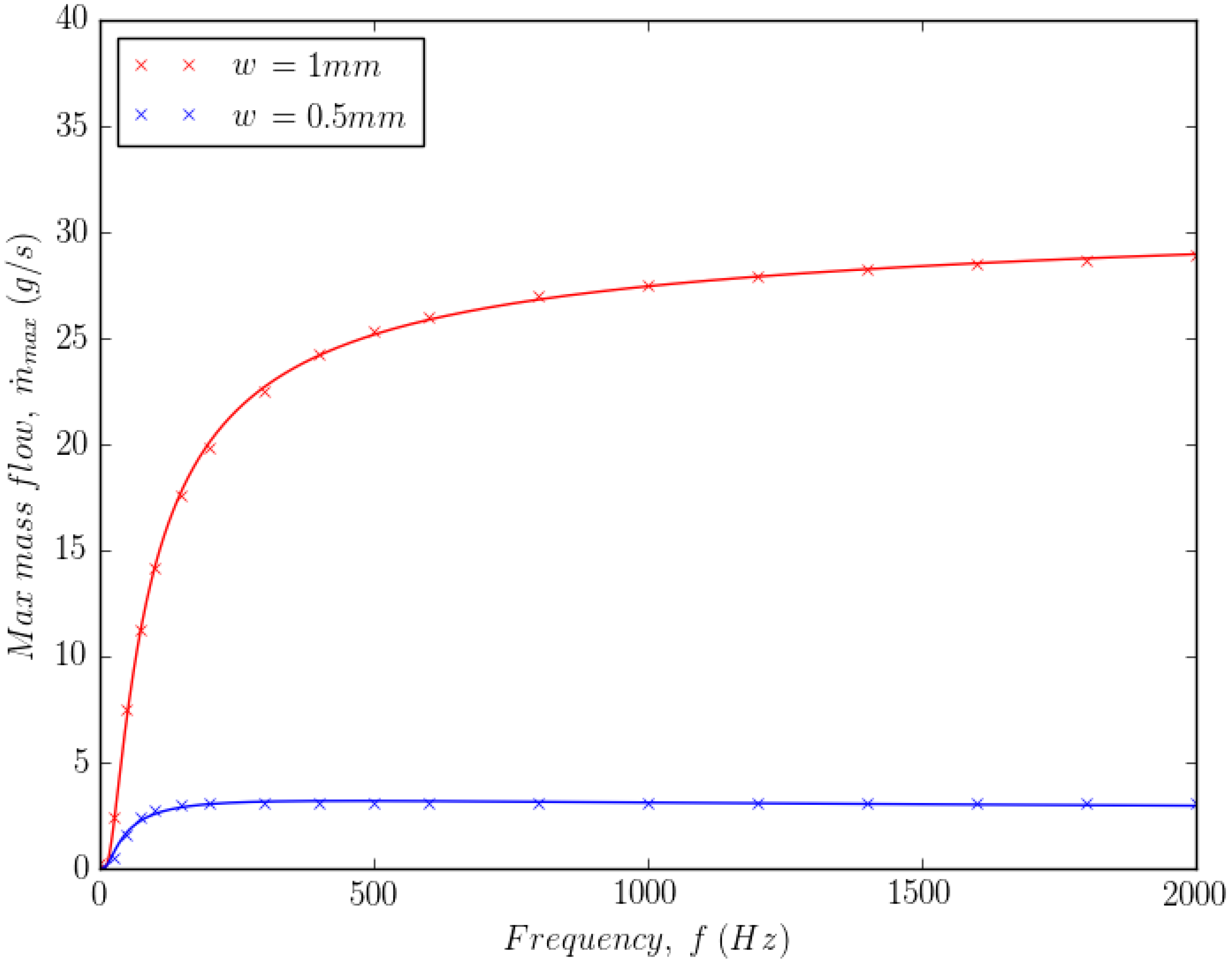
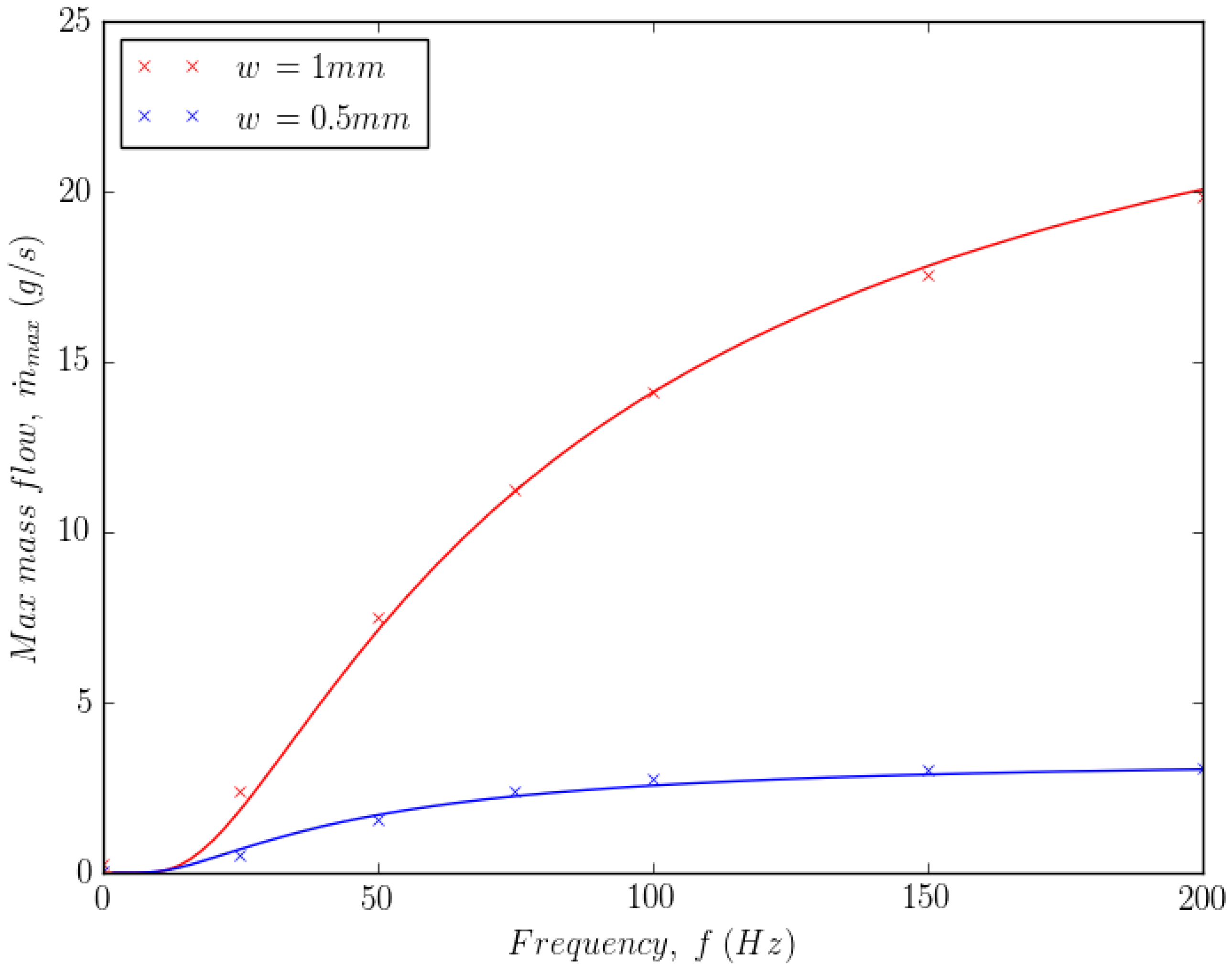
Figure 12 shows the maximum mass flow, , versus frequency, f, for two wall separations mm and mm. Equation (40) was used to fit the data. The fit suggests that the maximum mass flow tends to reach a limit at high frequency.
At high frequencies, the model behaves as expected, reaching a limit to the maximum mass flow. This limit is clearly larger for larger wall separations, as has been reported in the literature [66]. At low frequencies, Figure 13 shows that the continuum model shows a continuous reduction in the maximum mass flow. This is contrary to the sudden reduction shown in the literature for cohesive aluminium powder [66]. However, no results are available for non-cohesive Inconel powder. Nevertheless, these results may only be valid for type B powders such as unused Inconel 625. With cohesive type A powders, where the initial condition might include particle agglomeration, it is expected that a model of agglomeration and breakup would be required.
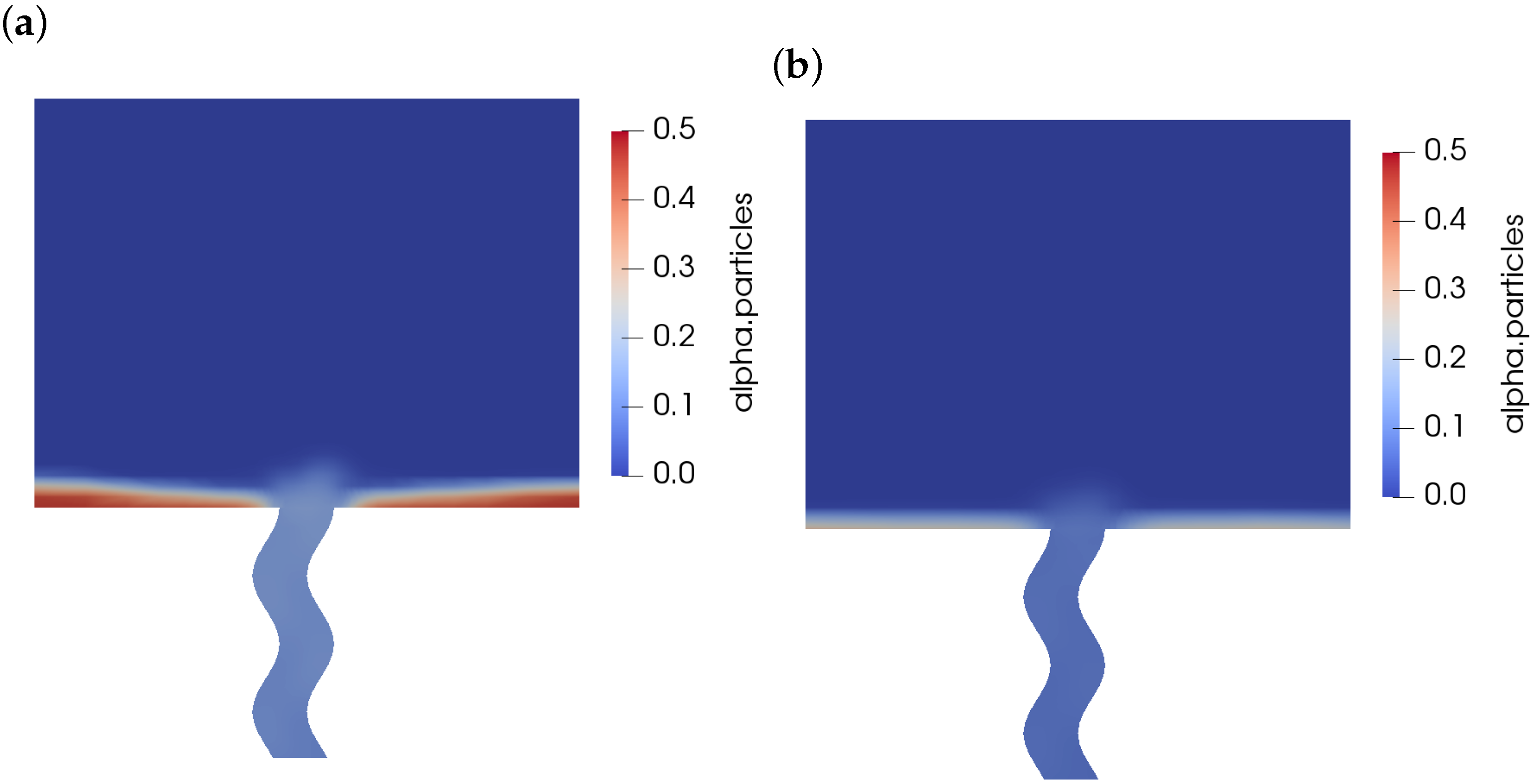
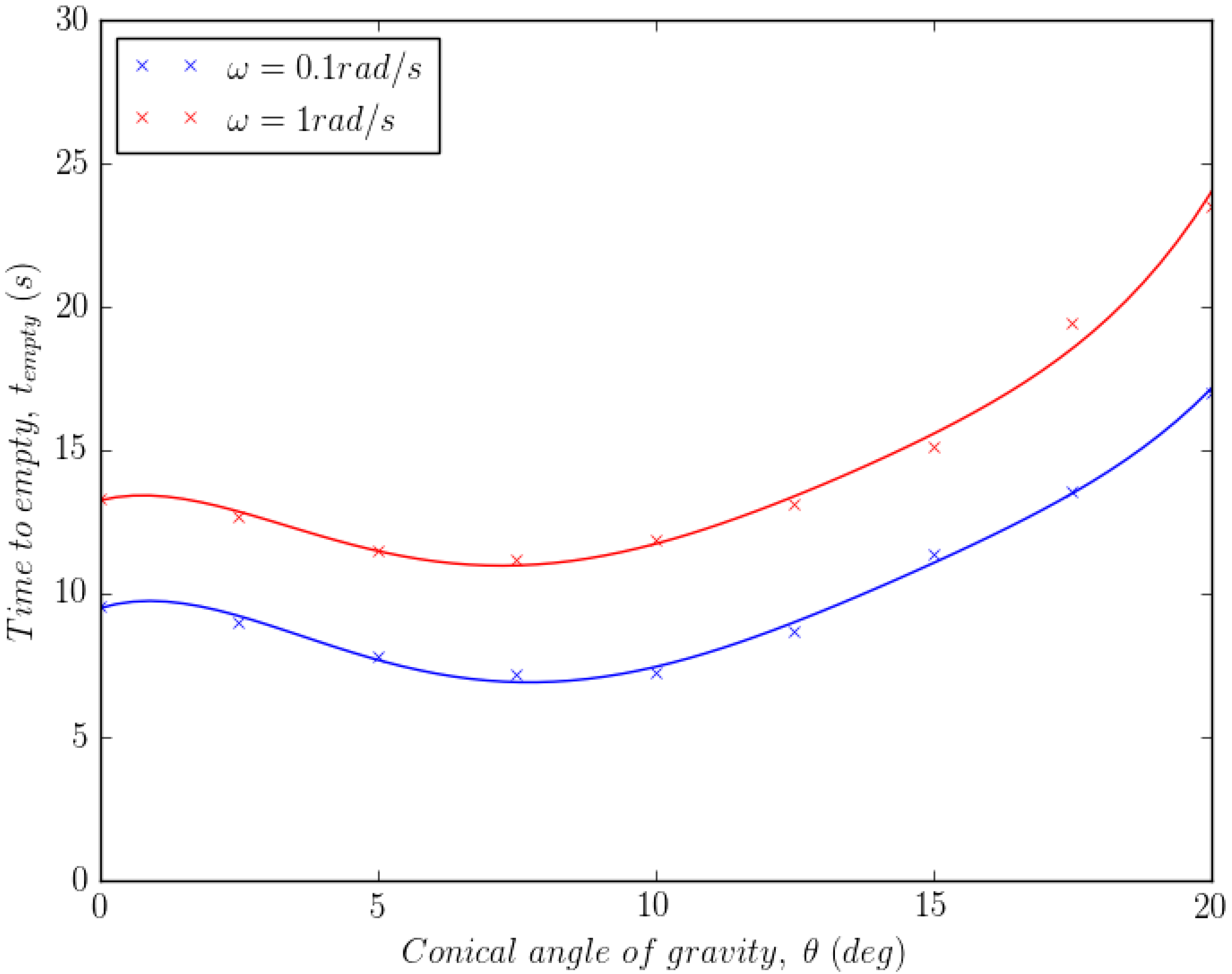
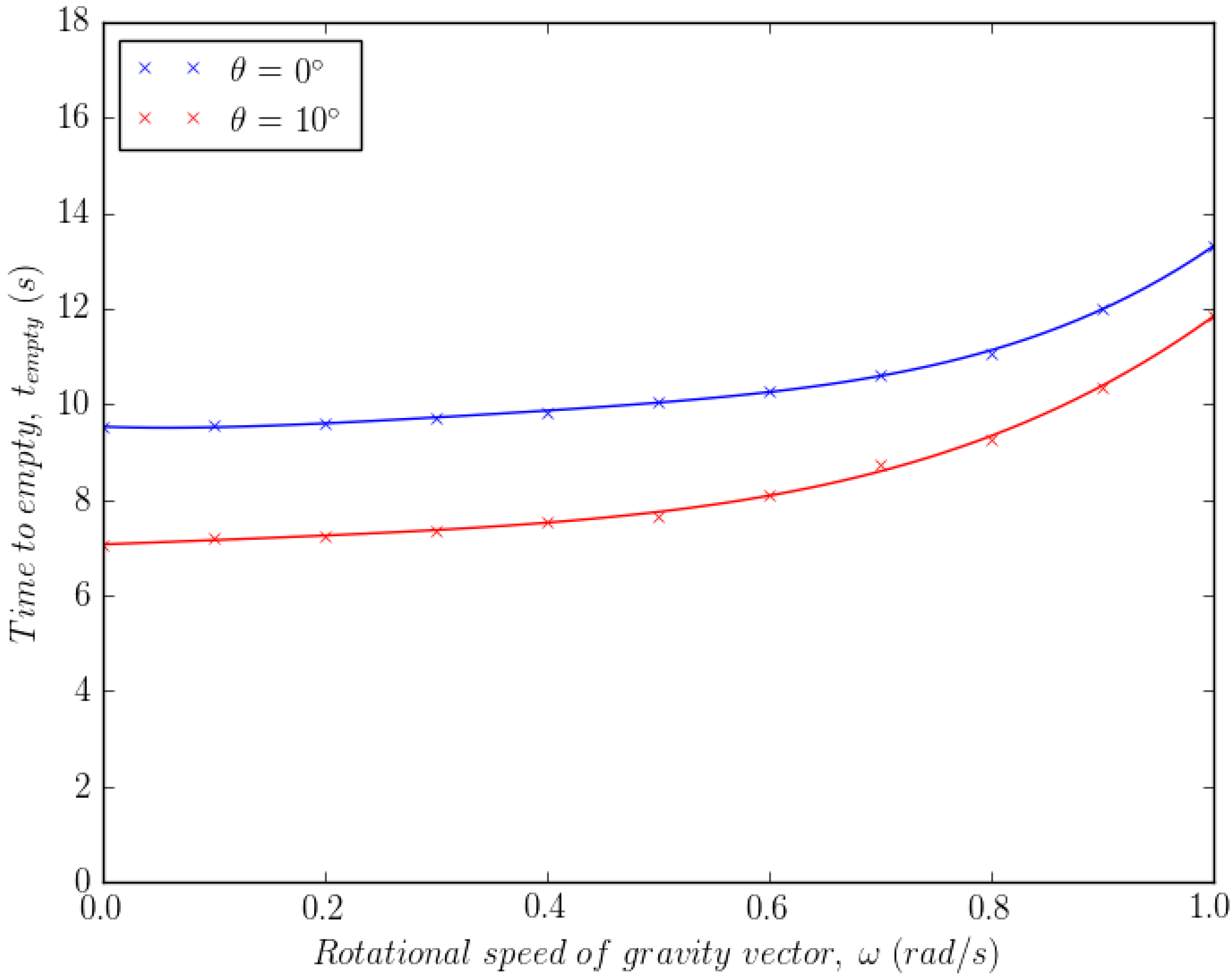
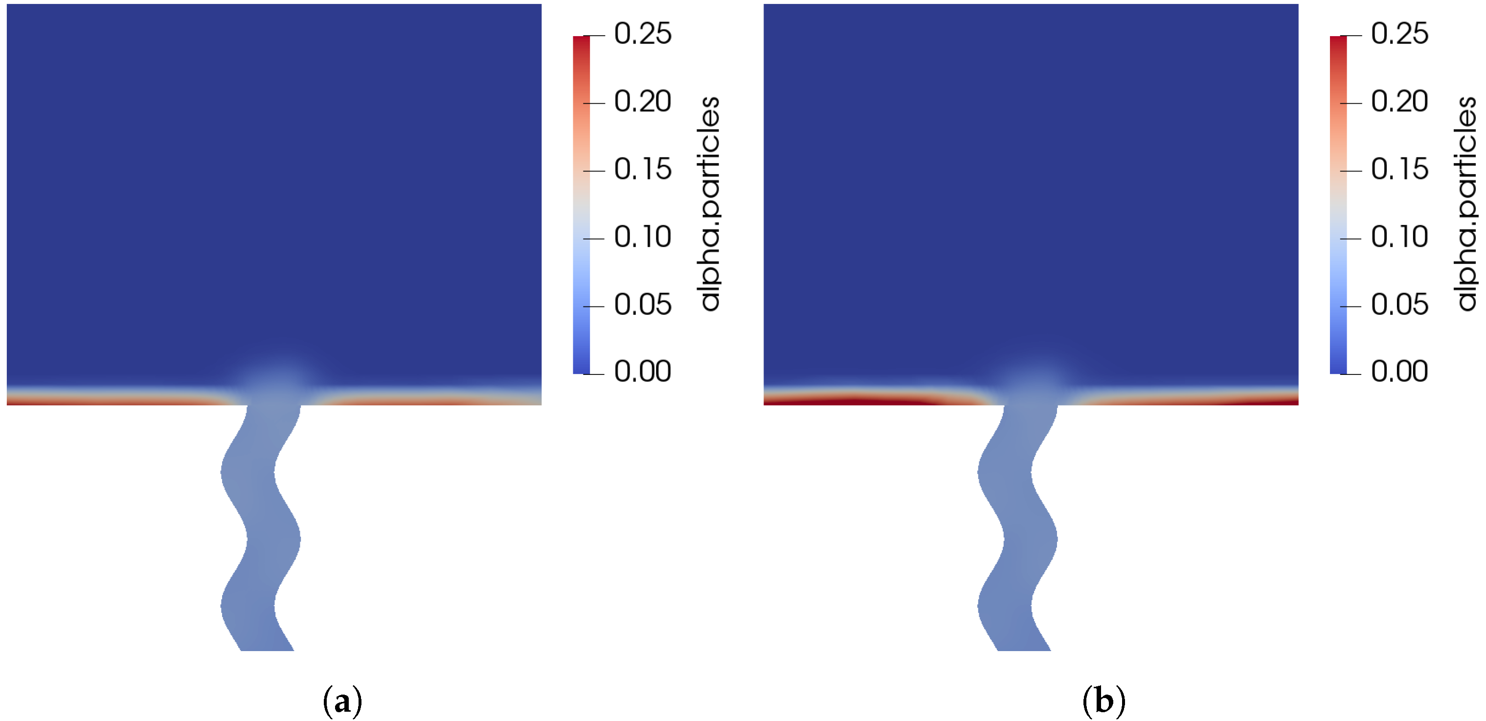
Figure 14 shows the time to empty plotted against the conical angle of gravity for two different rotational speeds and . For both speeds, it appears that a minimum time to empty is observed between an angle of and . This is because at , without an angle of gravity, powder is trapped in both corners of the device. At around , the angle is sufficiently large to empty the corners more quickly, whilst a larger angle such as traps powder in one corner more severely. Figure 15 plots the time to empty against the rotational speed of the gravity vector for two angles, and . For both angles it is clear that for rotational speeds of the order of , the emptying process is dominated by gravity, as the centrifugal acceleration is too small to have an influence. However, at higher rotational speeds the centrifugal acceleration increases the time to empty by sending particles away from the emptying orifice, as shown by Figure 16. Although it appears as though centrifugal forces are detrimental to powder removal, with a change in orientation, it may be possible to use them to empty powder from the device. In any case, more complex geometries are required in order to ascertain whether the manipulation sequence depends on the specific geometry in question.
5. Conclusions
Postprocessing of an AM-manufactured component is a key element of the manufacturing chain of AM, and can make a substantial difference to the physical behaviour of the component. With metal powder-based techniques such as PBF, one key aspect here is the removal of surplus powder from the internal structure of the component, where it might well affect the successful operation of that component (e.g., by blocking flow of fluid in a heat exchanger). This is typically achieved through vibrational fluidisation of the packed powder, allowing it to drain out of the component.
In this paper, we present a continuum model of the powder flow developed specifically to model this process. The individual models for aspects such as cohesion and vibration have been successfully validated against data from both the academic literature and against standard test cases. In particular, experimental data for the Hall flow test were used to validate the model of powder flow for Inconel and aluminium. The model of the wall vibration using a pseduo-heat flux boundary condition was also validated against experimental data from the literature. The limitations of these validations were that they dealt with un-used powder and also dealt with simple geometries that treated the wall vibration as a fixed frequency and amplitude across the whole of the geometry. Nevertheless, additional sub-models were proposed including a friction model that allowed strain-rate fluctuations, a conical gravity vector and a term for centrifugal acceleration.
A more complex test case was then developed based on a geometry proposed [63] for heat exchanger applications with the purpose of developing strategies for the manipulation sequence and energisation through wall-normal vibration. Several different wall separations for this wavy duct were investigated. The case also included sharp corners in the powder hopper in order to test out the manipulation sequence. To provide effective energisation, wall-normal vibration was provided in areas where the powder flow was restricted. This allowed powder feed to be controlled by the manipulation sequence and powder flow by the energisation. The manipulation sequence was found to be effective at removing powder trapped in the corners at the end of the emptying process, whilst the energisation dictated the maximum mass flow in the pseudo-steady region.
Trends in the maximum mass flow and time to empty revealed that a no-flow wall separation existed. In addition, the manipulation sequence had no influence on the maximum mass flow, which is instead directly determined by the magnitude of the RMS velocity of the wall-normal vibration. The time to empty was approximately equally affected by wall-normal vibration and by manipulation. However, the most effective strategy to minimise the time to empty was to combine wall-normal vibration with the manipulation sequence. Analysing the influence of vibration frequency on the maximum mass flow showed that the mass flow reaches a plateaux at high frequency as expected from the literature. However, the behaviour at low frequencies remains unvalidated. It was suggested that a diameter model could be used to introduced frequency dependent particle breakage for agglomerates in the case of a more cohesive powder. The time to empty was influenced by both the angle of the gravity vector and the rotational frequency. It was found that an optimum conical angle of gravity existed, whilst the influence of the rotational frequency of the manupiluation sequence tended to increase the time to empty. Further studies on this with more complex geometries might reveal different optimum sequences.
In these simulations, the RMS velocity has been assumed to be constant. This may be true for a very simple component, but over a complex component, the amplitude and frequency of the solid part is likely to vary. At the very least there may be a phase shift and amplitude shift between the solid part and the powder [67]. In addition, this modelling approach does not address any stresses present in the solid structure that may limit the frequencies that can be used. Coupling with a finite element model may provide such information. The CFD model requires the input of RMS velocity, which could be obtained from the RMS displacements of the FEA model. The FEA model would require the input of the time-varying mass of the powder, which could be obtained from the CFD model. It is also possible that this modelling could be extended to other powder types, for instance to include recycled powder whose physical properties may have changed [14], or powders used for Electron Beam Melting.
Author Contributions
Conceptualization, G.T., R.K. and D.B.; methodology, G.T., R.K. and A.R.; model development and validation, A.R.; analysis, A.R.; writing—original draft preparation, A.R. and G.T.; writing—review and editing, G.T.; supervision, G.T.; project administration, G.T. and D.B.; funding acquisition, G.T. and D.B. All authors have read and agreed to the published version of the manuscript.
Funding
This research was funded by InnovateUK and EPSRC under grant EP/P030785/1 “TACDAM; Tailorable and Adaptive Connected Digital Additive Manufacturing”.
Data Availability Statement
No data for public archival are reported in this study. This study does not report any data of this kind.
Conflicts of Interest
The authors declare no conflict of interest.
Abbreviations
The following abbreviations are used in this manuscript:
| AM | Additive Manufacture |
| CCM | Computational Continuum Mechanics |
| CFD | Computational Fluid Dynamics |
| DEM | Discrete Element Model |
| EBM | Electron Beam Melting |
| FE | Finite Element |
| FEA | Finite Element Analysis |
| FV | Finite Volume |
| MDM | Molecular Dynamics Model |
| PEEK | Polyether ether ketone |
| PEK | Polyetherketone |
| PBF | Powder Bed Fusion |
| SLM | Selective Laser Melting |
References
- ISO. ISO/ASTM52921-13: Standard Terminology for Additive Manufacturing—Coordinate Systems and Test Methodologies; ISO Subcommittee F42.01; ASTM International: West Conshohocken, PA, USA, 2019. [Google Scholar]
- Brighenti, R.; Cosma, M.P.; Marsavina, L.; Spagnoli, A.; Terzano, M. Laser-based additively manufactured polymers: A review on processes and mechanical models. J. Mater. Sci. 2021, 56, 961–998. [Google Scholar] [CrossRef]
- Grossin, D.; Montón, A.; Navarrete-Segado, P.; Özmen, E.; Urruth, G.; Maury, F.; Maury, D.; Frances, C.; Tourbin, M.; Lenormand, P.; et al. A review of additive manufacturing of ceramics by powder bed selective laser processing (sintering/melting): Calcium phosphate, silicon carbide, zirconia, alumina, and their composites. Open Ceram. 2021, 5, 100073. [Google Scholar] [CrossRef]
- Frazier, W.E. Metal additive manufacturing: A review. J. Mater. Eng. Perform. 2014, 23, 1917–1928. [Google Scholar] [CrossRef]
- Renishaw Plc. Investigating the Effects of Multiple Re-Use of Ti6Al4V Powder in Additive Manufacturing (AM). 2016. Available online: https://manufacturing.report/whitepapers/investigating-the-effects-of-multiple-re-use-of-ti6al4v-powder-in-additive-manufacturing (accessed on 5 August 2021).
- Vayre, B.; Vignat, F.; Villeneuve, F. Identification on some design key parameters for additive manufacturing: Application on Electron Beam Melting. Procedia CIRP 2013, 7, 264–269. [Google Scholar] [CrossRef] [Green Version]
- Dalquist, S.; Gutowski, T. Life Cycle Analysis of Conventional Manufacturing Techniques: Sand Casting. Manuf. Eng. Mater. Handl. Eng. 2004, 2004, 631–641. [Google Scholar] [CrossRef]
- MB Associates. Best Practice Guide for Foundry Sector of India; Bureau of Energy Efficiency (BEE) and Institute for Industrial Productivity (IIP): Kendal, UK, 2012. Available online: http://www.iipinetwork.org/resources/best-practice-guide-for-indias-foundry-sector (accessed on 5 August 2021).
- Duru, P.; Nicolas, M.; Hinch, J.; Guazzelli, E. Constitutive laws in liquid-fluidized beds. J. Fluid Mech 2002, 452, 371–404. [Google Scholar] [CrossRef] [Green Version]
- Guo, Y.; Curtis, J.S. Discrete Element Method Simulations for Complex Granular Flows. Annu. Rev. Fluid Mech. 2015, 47, 21–46. [Google Scholar] [CrossRef]
- Goldhirsch, I. Rapid granular flows. Ann. Rev. Fluid Mech 2003, 35, 267–293. [Google Scholar] [CrossRef]
- Bagnold, R.A. Experiments on a Gravity-Free Dispersion of Large Solid Spheres in a Newtonian Fluid under Shear. Proc. R. Soc. Lond. Ser. A Math. Phys. Sci. 1954, 225, 49–63. [Google Scholar] [CrossRef]
- Campbell, C.S. Granular material flows—An overview. Powder Technol. 2006, 162, 208–229. [Google Scholar] [CrossRef]
- Popov, V.V., Jr.; Katz-Demyanetz, A.; Garkun, A.; Bamberger, M. The effect of powder recycling on the mechanical properties and microstructure of electron beam melted Ti-6Al-4V specimens. Addit. Manuf. 2018, 22, 834–843. [Google Scholar]
- Aranson, I.S.; Tsimring, L.S. Patterns and collective behavior in granular media: Theoretical concepts. Rev. Mod. Phys. 2006, 78, 641–692. [Google Scholar] [CrossRef] [Green Version]
- Michopoulos, J.G.; Iliopoulos, A.P.; Steuben, J.C.; Birnbaum, A.J.; Lambrakos, S.G. On the multiphysics modeling challenges for metal additive manufacturing processes. Addit. Manuf. 2018, 22, 784–799. [Google Scholar] [CrossRef]
- Drikakis, D.; Frank, M.; Tabor, G. Multiscale Computational Fluid Dynamics. Energies 2019, 12, 3272. [Google Scholar] [CrossRef] [Green Version]
- Radjai, F.; Roux, J.N.; Daouadji, A. Modeling Granular Materials: Century-Long Research across Scales. J. Eng. Mech. 2017, 143, 04017002. [Google Scholar] [CrossRef] [Green Version]
- Aranson, I. Granular Patterns; Oxford University Press: Oxford, UK, 2009. [Google Scholar]
- Durst, F.; Milojevic, F.; Schönung, B. Eulerian and lagrangian predicitons of particulate two-phase flows: A numerical study. Appl. Math. Model. 1984, 8, 101–115. [Google Scholar] [CrossRef]
- Da Cruz, F.; Emam, S.; Prochnow, M.; Roux, J.N.; Chevoir, F. Rheophysics of dense granular materials: Discrete simulation of plane shear flows. Phys. Rev. E Stat. Nonlinear Soft Matter Phys. 2005, 72, 1–17. [Google Scholar] [CrossRef] [Green Version]
- Rognon, P.G.; Roux, J.N.; Naaïm, M.; Chevoir, F. Dense flows of cohesive granular materials. J. Fluid Mech. 2008, 596, 21–47. [Google Scholar] [CrossRef] [Green Version]
- Jop, P.; Forterre, Y.; Pouliquen, O. A constitutive law for dense granular flows. Nature 2006, 441, 727–730. [Google Scholar] [CrossRef] [Green Version]
- Passalacqua, A.; Fox, R.O. Implementation of an iterative solution procedure for multi-fluid gas-particle flow models on unstructured grids. Powder Technol. 2011, 213, 174–187. [Google Scholar] [CrossRef]
- Srivastava, A.; Sundaresan, S. Analysis of a frictional-kinetic model for gas-particle flow. Powder Technol. 2003, 129, 72–85. [Google Scholar] [CrossRef]
- Zheng, Q.; Yu, A. Finite element investigation of the flow and stress patterns in conical hopper during discharge. Chem. Eng. Sci. 2015, 129, 49–57. [Google Scholar] [CrossRef]
- Liu, S.; Zhou, Z.; Zou, R.; Pinson, D.; Yu, A. Flow characteristics and discharge rate of ellipsoidal particles in a flat bottom hopper. Powder Technol. 2014, 253, 70–79. [Google Scholar] [CrossRef]
- Bharadwaj, R.; Khambekar, J.; Orlando, A.; Gao, Z.; Shen, H.; Helenbrook, B.; Royal, T.A.; Weitzman, P. A Comparison of Discrete Element Modeling, Finite Element Analysis, and Physical Experiment of Granular Material Systems in a Direct Shear Cell. AIP Conf. Proc. 2008, 969, 221–228. [Google Scholar] [CrossRef]
- Liu, Y.; Gonzalez, M.; Wassgren, C. Modeling granular material blending in a rotating drum using a finite element method and advection-diffusion equation multiscale model. AIChE J. 2018, 64, 3277–3292. [Google Scholar] [CrossRef] [Green Version]
- Chen, H.; Wei, Q.; Wen, S.; Li, Z.; Shi, Y. Flow behavior of powder particles in layering process of selective laser melting: Numerical modeling and experimental verification based on discrete element method. Int. J. Mach. Tools Manuf. 2017, 123, 146–159. [Google Scholar] [CrossRef]
- Fouda, Y.M.; Bayly, A.E. A DEM study of powder spreading in additive layer manufacturing. Granul. Matter 2020, 22, 10. [Google Scholar] [CrossRef] [Green Version]
- Haeri, S.; Wang, Y.; Ghita, O.; Sun, J. Discrete element simulation and experimental study of powder spreading process in additive manufacturing. Powder Technol. 2016, 306, 45–54. [Google Scholar] [CrossRef] [Green Version]
- Plimpton, S. Fast parallel algorithms for short-range molecular dynamics. J. Comput. Phys. 1995, 117, 1–19. [Google Scholar] [CrossRef] [Green Version]
- Johanson, J.R. A Rolling Theory for Granular Solids. J. Appl. Mech. 1965, 32, 842–848. [Google Scholar] [CrossRef]
- Dec, R.T.; Zavaliangos, A.; Cunningham, J.C. Comparison of various modeling methods for analysis of powder compaction in roller press. Powder Technol. 2003, 130, 265–271. [Google Scholar] [CrossRef]
- Shanjani, Y.; Toyserkani, E. Material spreading and compaction in powder-based solid freeform fabrication methods: Mathematical modeling. In Proceedings of the 19th Annual International Solid Freeform Fabrication Symposium, Austin, TX, USA, 4–8 August 2008; pp. 399–410. [Google Scholar]
- Desai, P.S.; Higgs, C.F. Spreading Process Maps for Powder-Bed Additive Manufacturing Derived from Physics Model-Based Machine Learning. Metals 2019, 9, 1176. [Google Scholar] [CrossRef] [Green Version]
- Martin, S.; Guessasma, M.; Léchelle, J.; Fortin, J.; Saleh, K.; Adenot, F. Simulation of sintering using a Non Smooth Discrete Element Method. Application to the study of rearrangement. Comput. Mater. Sci. 2014, 84, 31–39. [Google Scholar] [CrossRef]
- Martin, S.; Parekh, R.; Guessasma, M.; Léchelle, J.; Fortin, J.; Saleh, K. Study of the sintering kinetics of bimodal powders. A parametric DEM study. Powder Technol. 2015, 270, 637–645. [Google Scholar] [CrossRef]
- Xin, H.; Sun, W.; Fish, J. Discrete element simulations of powder-bed sintering-based additive manufacturing. Int. J. Mech. Sci. 2018, 149, 373–392. [Google Scholar] [CrossRef]
- Wei, H.; Mukherjee, T.; Zhang, W.; Zuback, J.; Knapp, G.; De, A.; DebRoy, T. Mechanistic models for additive manufacturing of metallic components. Prog. Mater. Sci. 2021, 116, 100703. [Google Scholar] [CrossRef]
- Steuben, J.C.; Iliopoulos, A.P.; Michopoulos, J.G. On Multiphysics Discrete Element Modeling of Powder-Based Additive Manufacturing Processes. In Proceedings of the ASME 2016 International Design Engineering Technical Conferences & Computers and Information in Engineering Conference, IDETC/CIE, Charlotte, NC, USA, 21–24 August 2016. [Google Scholar]
- Kloss, C.; Goniva, C.; Hager, A.; Amberger, S.; Pirker, S. Models, algorithms and validation for opensource DEM and CFD-DEM. Prog. Comput. Fluid Dyn. 2012, 12, 140–152. [Google Scholar] [CrossRef]
- Lee, W.H.; Zhang, Y.; Zhang, J. Discrete element modeling of powder flow and laser heating in direct metal laser sintering process. Powder Technol. 2017, 315, 300–308. [Google Scholar] [CrossRef] [Green Version]
- Ibarra-Medina, J.; Pinkerton, A. A numerical investigation of powder heating in coaxial laser metal deposition. In Proceedings of the 36th International MATADOR Conference; Springer: London, UK, 2010. [Google Scholar] [CrossRef]
- Pan, H.; Sparks, T.; Thakar, Y.D.; Liou, F. The Investigation of Gravity-Driven Metal Powder Flow in Coaxial Nozzle for Laser-Aided Direct Metal Deposition Process. J. Manuf. Sci. Eng. 2005, 128, 541–553. [Google Scholar] [CrossRef]
- Zeng, Q.; Tian, Y.; Xu, Z.; Qin, Y. Numerical modelling of the gas-powder flow during the laser metal deposition for additive manufacturing. In Proceedings of the 15 International Conference on Manufacturing Research, London, UK, 5–7 September 2017. [Google Scholar]
- Morimoto, K.; Suzuki, Y.; Kasagi, N. Mechanism of Heat Transfer Enhancement in Recuperators with Oblique Wavy Walls. Therm. Sci. Eng. 2004, 12, 99–100. [Google Scholar]
- Riella, M.; Kahraman, R.; Tabor, G. Reynolds-Averaged Two-Fluid Model prediction of moderately dilute fluid-particle flow over a backward-facing step. Int. J. Multiph. Flow 2018, 106, 95–108. [Google Scholar] [CrossRef] [Green Version]
- Riella, M.; Kahraman, R.; Tabor, G. Inhomogeneity and anisotropy in Eulerian–Eulerian near-wall modelling. Int. J. Multiph. Flow 2019, 114, 9–18. [Google Scholar] [CrossRef]
- Van Wachem, B.G.M. Derivation, Implementation, and Validation of Computer Simulation Models for Gas-Solid Fluidized Beds. Ph.D. Thesis, Delft University of Technology (TU Delft), Delft, The Netherlands, 2000. [Google Scholar]
- Geldart, D. Types of gas fluidization. Powder Technol. 1973, 7, 285–292. [Google Scholar] [CrossRef]
- ASTM B213-20. Standard Test Methods for Flow Rate of Metal Powders Using the Hall Flowmeter; ASTM International: West Conshohocken, PA, USA, 2020. [Google Scholar]
- Gidaspow, D.; Huilin, L. Equation of State and Radial Distribution Functions of FCC Particles in a CFB. AIChE J. 1998, 44, 279–293. [Google Scholar] [CrossRef]
- Van Wachem, B.; Sasic, S. Derivation, simulation and validation of a cohesive particle flow CFD model. AIChE J. 2008, 54, 9–19. [Google Scholar] [CrossRef] [Green Version]
- Ocone, R.; Goodwin, J.; Delebarre, A. Flow structures of Geldart A solids in circulating fluidized beds. Chem. Eng. Res. Des. 2000, 6, 860–865. [Google Scholar] [CrossRef]
- Makkawi, Y.T.; Wright, P.C.; Ocone, R. The effect of friction and inter particle cohesive forces on the hydrodynamics of gas solid flow. A comparative analysis of theoretical predictions and experiments. Powder Technol. 2006, 163, 69–79. [Google Scholar] [CrossRef]
- Vlachos, N.; Chang, I.T.H. Investigation of flow properties of metal powders from narrow particle size distribution to polydisperse mixtures through an improved Hall flowmeter. Powder Technol. 2011, 205, 71–80. [Google Scholar] [CrossRef]
- Kamenetskii, E.S.; Orlova, N.S.; Tagirov, A.M.; Volik, M.V. Three-Dimensional Simulation of a Vibrofluidized Bed with the Use of a Two-Fluid Model of Granular Gas. J. Eng. Phys. Thermophys. 2016, 89, 1459–1465. [Google Scholar] [CrossRef]
- Richman, M.W. Boundary conditions for granular flows at randomly fluctuating bumpy boundaries. Mech. Mater. 1993, 16, 211–218. [Google Scholar] [CrossRef]
- Viswanathan, H.; Sheikh, N.A.; Wildman, R.D.; Huntley, J.M. Convection in three-dimensional vibrofluidized granular beds. J. Fluid Mech. 2011, 682, 185–212. [Google Scholar] [CrossRef] [Green Version]
- Orlova, N.S. Comparison of the results of experimental investigations of a vibrofluidized bed with caluclations by a granular gas hydrodynamic model. J. Eng. Phys. Thermophys. 2014, 87, 429–435. [Google Scholar] [CrossRef]
- Morimoto, K.; Suzuki, Y.; Kasagi, N. Optimal Shape Design of Compact Heat Exchangers based on Adjoint Analysis of Momentum and Heat Transfer. J. Therm. Sci. Technol. 2010, 5, 24–35. [Google Scholar] [CrossRef] [Green Version]
- Kahraman, R.; Bacheva, D.; Schmieder, A.; Tabor, G.R. Coupling of Volume of Fluid and Level Set Methods in Condensing Heat Transfer Simulations. Int. J. Comput. Fluid Dyn. 2019, 34, 25–38. [Google Scholar] [CrossRef]
- Gledhill, I.M.A.; Roohani, H.; Forsberg, K.; Eliasson, P.; Skews, B.W.; Nordström, J. Theoretical treatment of fluid flow for accelerating bodies. Theor. Comput. Fluid Dyn. 2016, 30, 449–467. [Google Scholar] [CrossRef] [Green Version]
- Matsusaka, S.; Yamamoto, K.; Masuda, H. Micro-feeding of a fine powder using a vibrating capillary tube. Adv. Powder Technol. 1996, 7, 141–151. [Google Scholar] [CrossRef]
- Kroll, V.W. Uber das Verhalien von Schüttgut in lotrecht schwingenden Gefessen. Forschung auf dem Gebiete des Ingenieurwesens 1954, 20, 2–15. [Google Scholar]
Figure 1.
Basic geometry and boundary conditions for the Hallflow case (2D representation). Note that this is a conical shape hopper; the full 3D geometry is constructed from rotation around the central axis.
Figure 1.
Basic geometry and boundary conditions for the Hallflow case (2D representation). Note that this is a conical shape hopper; the full 3D geometry is constructed from rotation around the central axis.

Figure 2.
Comparison between the Eulerian–Eulerian model and the Hallflow experimental data. (a) Results for Inconel (Geldart Type B) without cohesive force model. (b) Results for aluminium powder (Geldart Type A) with different values of .
Figure 2.
Comparison between the Eulerian–Eulerian model and the Hallflow experimental data. (a) Results for Inconel (Geldart Type B) without cohesive force model. (b) Results for aluminium powder (Geldart Type A) with different values of .

Figure 3.
Square geometry used to validate the vibration modelling. (a) With sinusoidally varying gravity body force, (b) With pseudo-heat flux boundary on granular temperature.
Figure 3.
Square geometry used to validate the vibration modelling. (a) With sinusoidally varying gravity body force, (b) With pseudo-heat flux boundary on granular temperature.

Figure 4.
Effect of frequency on solid volume fraction field.

Figure 5.
Different modelling techniques for vibration: (a) with gravity body force and (b) with wall-normal heat flux.
Figure 5.
Different modelling techniques for vibration: (a) with gravity body force and (b) with wall-normal heat flux.

Figure 6.
Validation of wall-normal vibration model. (a) mm, (b) mm.

Figure 7.
Morimoto geometry and boundary conditions. (a) A schematic in 2D showing the boundary conditions and gravity vector; (b) half the domain in 3D to further aid understanding. The section in red is set as a vibrating wall.
Figure 7.
Morimoto geometry and boundary conditions. (a) A schematic in 2D showing the boundary conditions and gravity vector; (b) half the domain in 3D to further aid understanding. The section in red is set as a vibrating wall.

Figure 8.
Effect of manipulation sequence on the volume fraction field. (a) mm at s, no vibration, no manipulation; (b) mm at s, no vibration, , .
Figure 8.
Effect of manipulation sequence on the volume fraction field. (a) mm at s, no vibration, no manipulation; (b) mm at s, no vibration, , .

Figure 9.
Effect of manipulation sequence.

Figure 10.
Effect of manipulation and wall-normal vibration.

Figure 11.
Effect of manipulation sequence and vibration on the volume fraction field. (a) mm at s, mm, no manipulation. (b) mm at s, mm, , .
Figure 11.
Effect of manipulation sequence and vibration on the volume fraction field. (a) mm at s, mm, no manipulation. (b) mm at s, mm, , .

Figure 12.
Maximum mass flow versus frequency at high frequencies.

Figure 13.
Maximum mass flow versus frequency at low frequencies.

Figure 14.
Time to empty versus angle of gravity vector.

Figure 15.
Time to empty versus rotational speed of gravity vector.

Figure 16.
Effect of the rotational speed of the gravity vector on the volume fraction field. (a) mm at t = 5 s, Hz, mm, deg, rad/s. (b) mm at t = 5 s, f = 20 Hz, a = 1.25 mm, = 10 deg, = 1 rad/s.
Figure 16.
Effect of the rotational speed of the gravity vector on the volume fraction field. (a) mm at t = 5 s, Hz, mm, deg, rad/s. (b) mm at t = 5 s, f = 20 Hz, a = 1.25 mm, = 10 deg, = 1 rad/s.

Publisher’s Note: MDPI stays neutral with regard to jurisdictional claims in published maps and institutional affiliations. |
© 2021 by the authors. Licensee MDPI, Basel, Switzerland. This article is an open access article distributed under the terms and conditions of the Creative Commons Attribution (CC BY) license (https://creativecommons.org/licenses/by/4.0/).
Share and Cite
MDPI and ACS Style
Roberts, A.; Kahraman, R.; Bacheva, D.; Tabor, G. Modelling of Powder Removal for Additive Manufacture Postprocessing. J. Manuf. Mater. Process. 2021, 5, 86. https://doi.org/10.3390/jmmp5030086
AMA Style
Roberts A, Kahraman R, Bacheva D, Tabor G. Modelling of Powder Removal for Additive Manufacture Postprocessing. Journal of Manufacturing and Materials Processing. 2021; 5(3):86. https://doi.org/10.3390/jmmp5030086
Chicago/Turabian StyleRoberts, Andrew, Recep Kahraman, Desi Bacheva, and Gavin Tabor. 2021. "Modelling of Powder Removal for Additive Manufacture Postprocessing" Journal of Manufacturing and Materials Processing 5, no. 3: 86. https://doi.org/10.3390/jmmp5030086