
Robust Measures of Image-Registration-Derived Lung Biomechanics in SPIROMICS
 , , , and
Abstract
:1. Introduction
2. Materials and Methods
2.1. Data
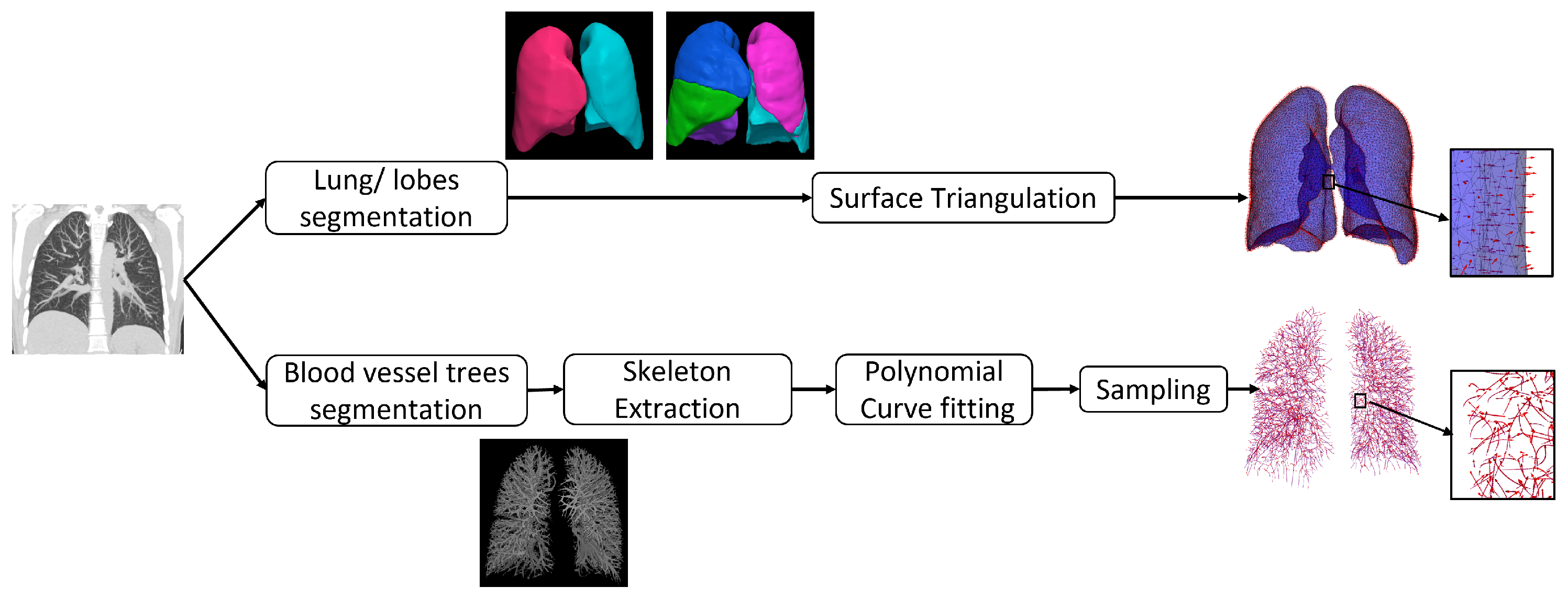
2.2. Preprocessing
2.3. Image Registration Algorithms
2.3.1. SSTVD
2.3.2. GDR
2.3.3. GSyN
2.3.4. PVSV
2.3.5. PLOSL
2.4. Image Registration Parameters
2.5. Image Registration Performance
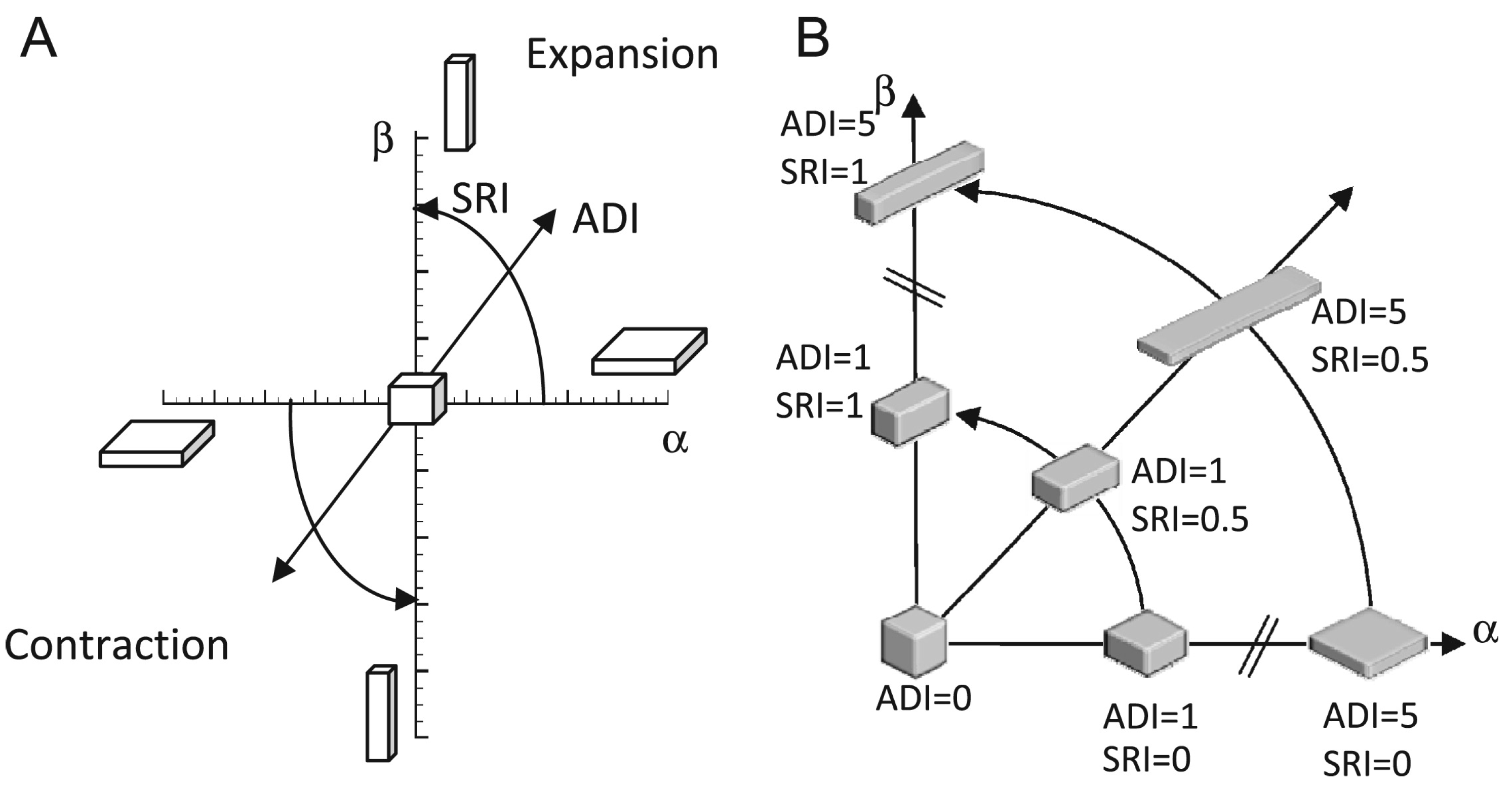
2.6. Biomechanical Measures
3. Results
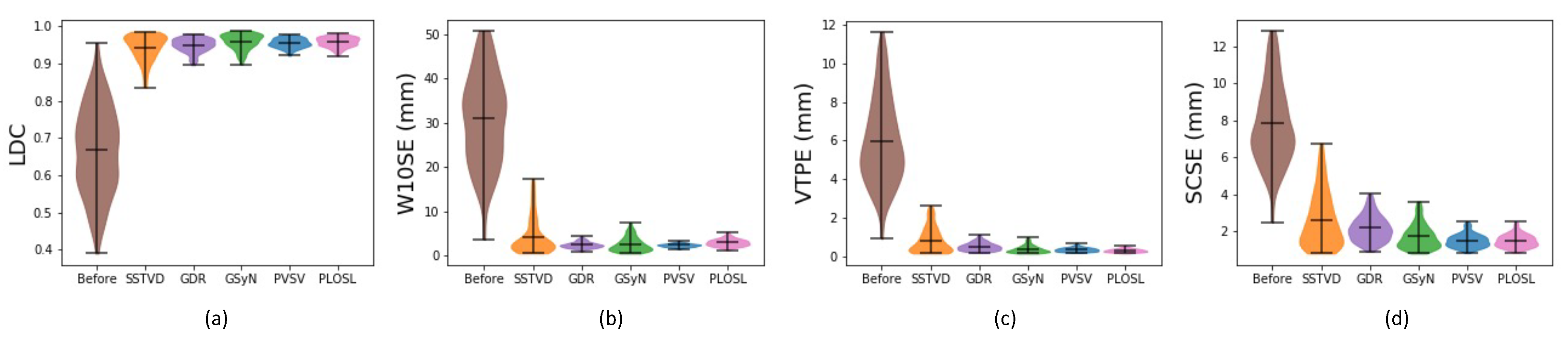
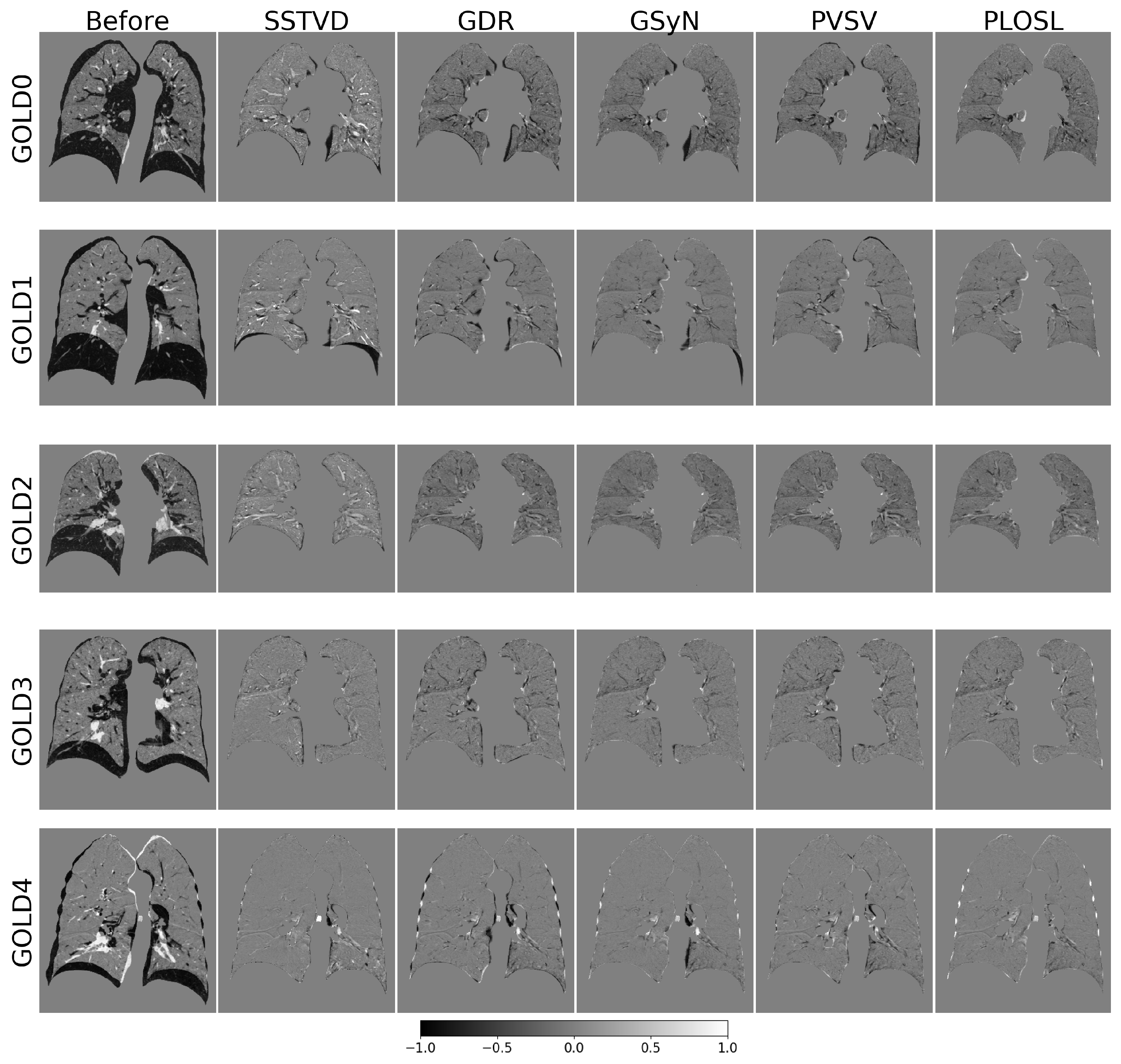
3.1. Registration Performance
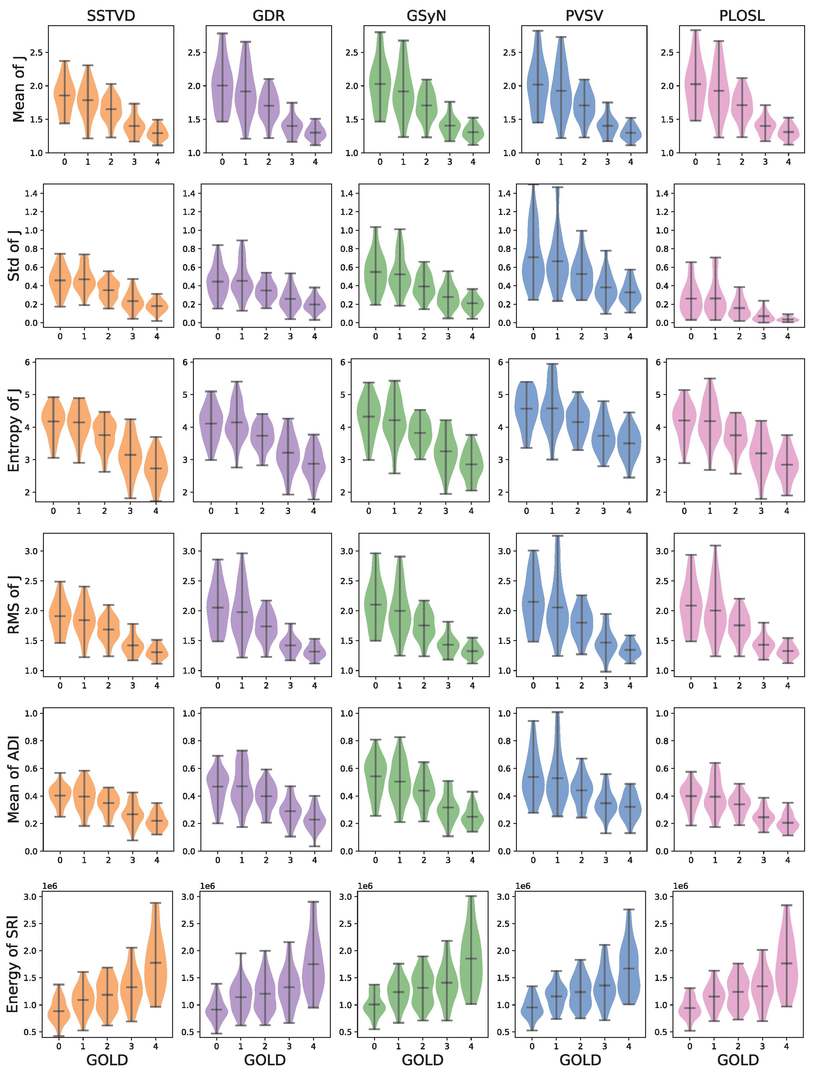
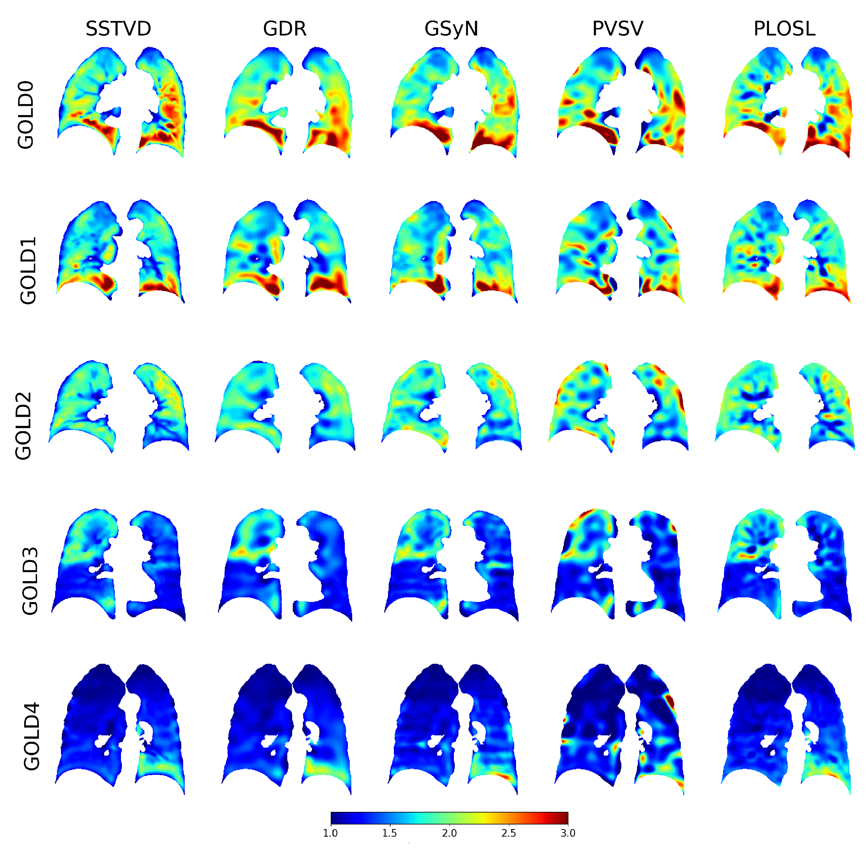
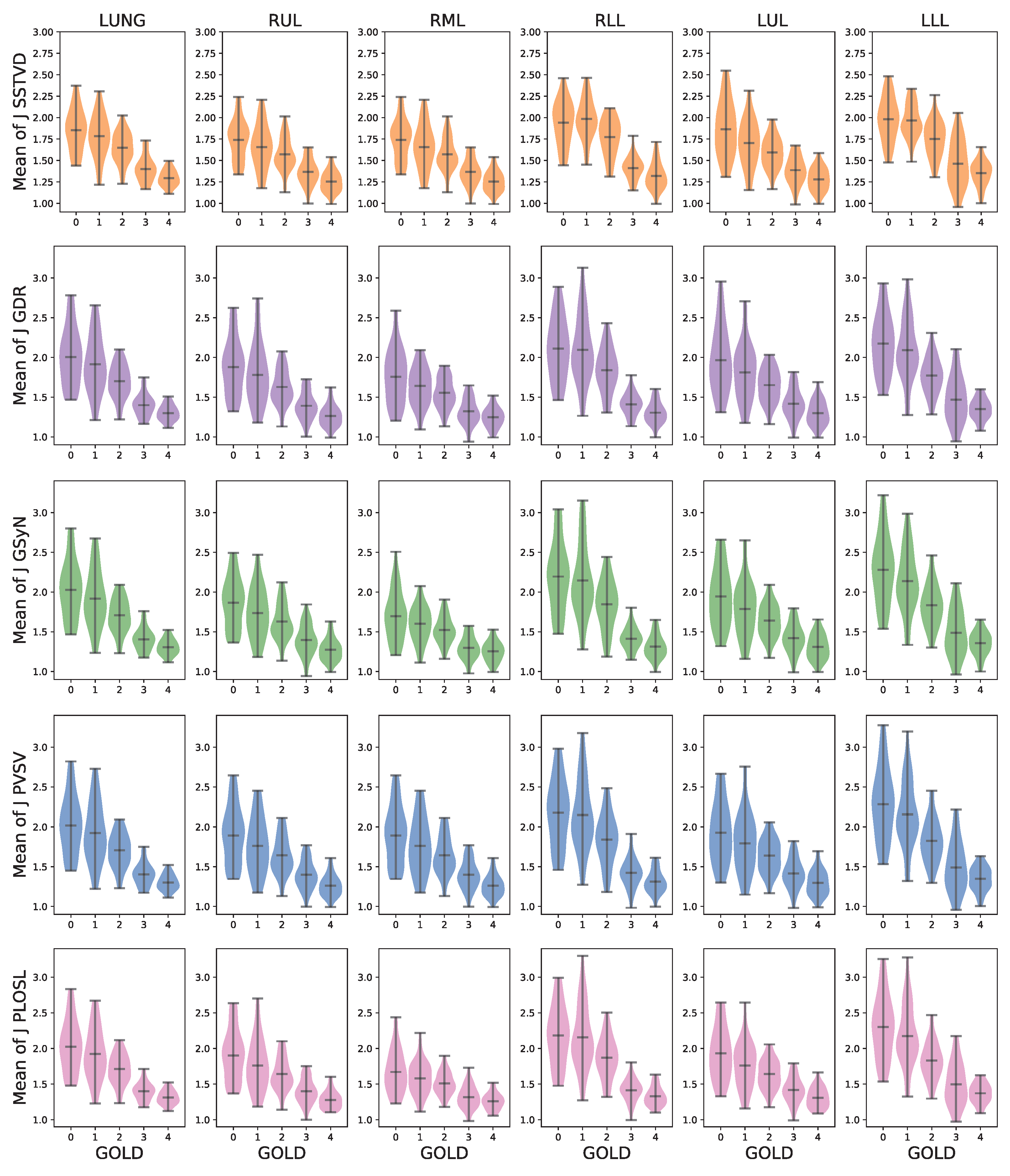
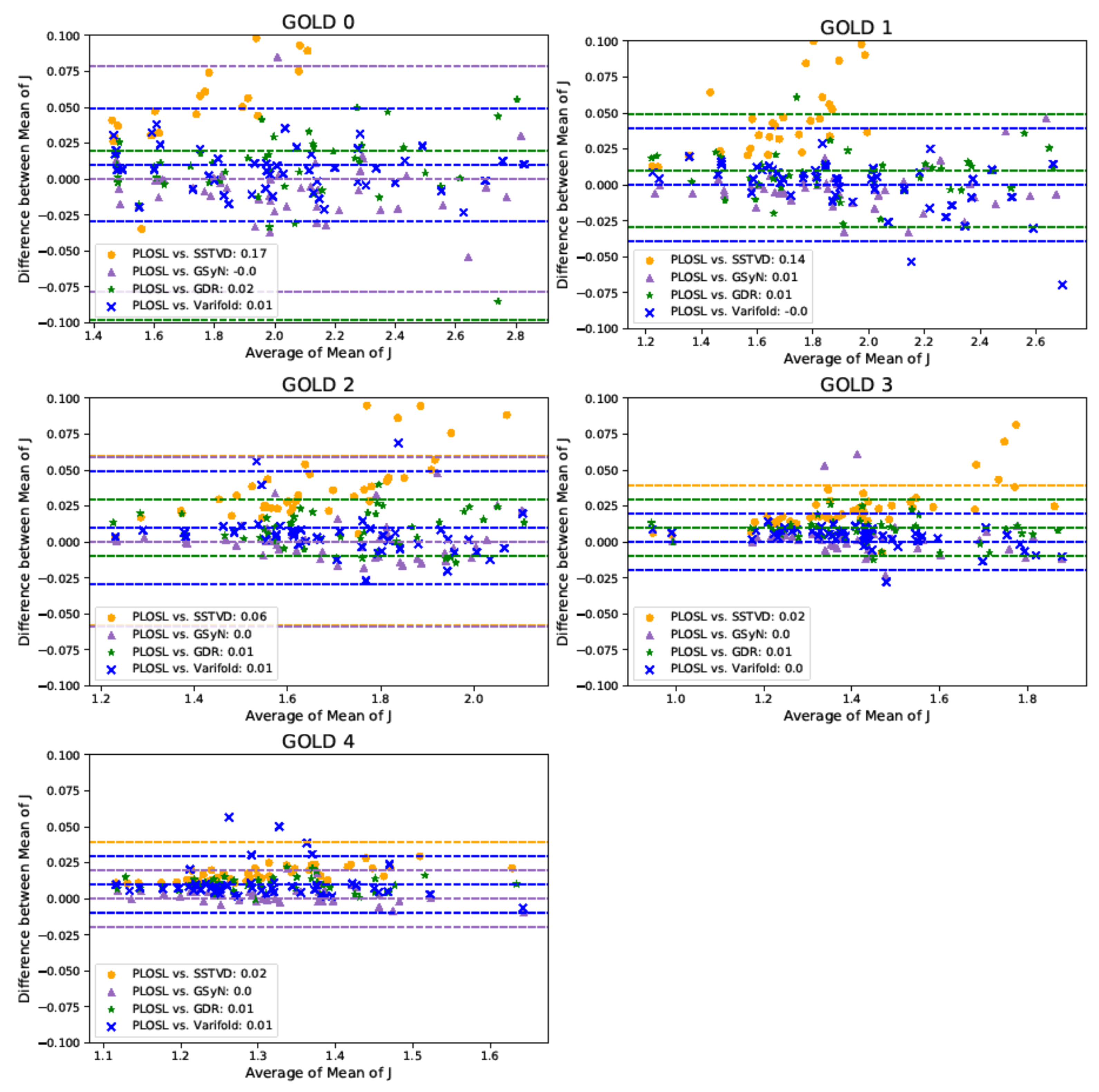
3.2. Robustness of Inferred Biomechanical Features
4. Discussion and Conclusions
Author Contributions
Funding
Institutional Review Board Statement
Informed Consent Statement
Data Availability Statement
Acknowledgments
Conflicts of Interest
Appendix A. Quantitative Results for Figure

| Biomechanical Measure | Method | GOLD 0 | GOLD 1 | GOLD 2 | GOLD 3 | GOLD 4 |
|---|---|---|---|---|---|---|
| Mean of J | SSTVD | 1.85 ± 0.24 | 1.78 ± 0.24 | 1.65 ± 0.17 | 1.40 ± 0.14 | 1.29 ± 0.09 |
| GDR | 2.01 ± 0.36 | 1.92 ± 0.35 | 1.70 ± 0.20 | 1.40 ± 0.14 | 1.30 ± 0.09 | |
| GSyN | 2.03 ± 0.35 | 1.92 ± 0.35 | 1.71 ± 0.20 | 1.40 ± 0.14 | 1.31 ± 0.10 | |
| PVSV | 2.02 ± 0.36 | 1.93 ± 0.36 | 1.71 ± 0.21 | 1.40 ± 0.14 | 1.30 ± 0.09 | |
| PLOSL | 2.03 ± 0.36 | 1.92 ± 0.35 | 1.71 ± 0.20 | 1.40 ± 0.12 | 1.31 ± 0.09 | |
| Std of J | SSTVD | 0.46 ± 0.13 | 0.47 ± 0.13 | 0.35 ± 0.10 | 0.23 ± 0.10 | 0.18 ± 0.06 |
| GDR | 0.44 ± 0.16 | 0.45 ± 0.17 | 0.35 ± 0.10 | 0.26 ± 0.11 | 0.20 ± 0.07 | |
| GSyN | 0.55 ± 0.20 | 0.52 ± 0.19 | 0.39 ± 0.12 | 0.28 ± 0.12 | 0.21 ± 0.07 | |
| PVSV | 0.71 ± 0.29 | 0.66 ± 0.29 | 0.53 ± 0.18 | 0.38 ± 0.15 | 0.33 ± 0.11 | |
| PLOSL | 0.26 ± 0.16 | 0.26 ± 0.19 | 0.16 ± 0.10 | 0.07 ± 0.05 | 0.04 ± 0.02 | |
| Entropy of J | SSTVD | 4.17 ± 0.45 | 4.15 ± 0.46 | 3.75 ± 0.43 | 3.15 ± 0.56 | 2.73 ± 0.45 |
| GDR | 4.11 ± 0.50 | 4.14 ± 0.54 | 3.73 ± 0.38 | 3.21 ± 0.54 | 2.88 ± 0.45 | |
| GSyN | 4.32 ± 0.57 | 4.21 ± 0.63 | 3.82 ± 0.39 | 3.26 ± 0.53 | 2.85 ± 0.43 | |
| PVSV | 4.57 ± 0.53 | 4.58 ± 0.68 | 4.16 ± 0.43 | 3.73 ± 0.46 | 3.50 ± 0.43 | |
| PLOSL | 4.21 ± 0.50 | 4.18 ± 0.59 | 3.75 ± 0.42 | 3.20 ± 0.56 | 2.85 ± 0.45 | |
| RMS of J | SSTVD | 1.91 ± 0.26 | 1.84 ± 0.27 | 1.69 ± 0.19 | 1.42 ± 0.16 | 1.31 ± 0.10 |
| GDR | 2.05 ± 0.36 | 1.98 ± 0.39 | 1.74 ± 0.22 | 1.42 ± 0.15 | 1.32 ± 0.10 | |
| GSyN | 2.10 ± 0.39 | 2.00 ± 0.39 | 1.75 ± 0.22 | 1.43 ± 0.15 | 1.33 ± 0.10 | |
| PVSV | 2.15 ± 0.41 | 2.06 ± 0.47 | 1.80 ± 0.25 | 1.47 ± 0.22 | 1.35 ± 0.12 | |
| PLOSL | 2.09 ± 0.38 | 2.01 ± 0.41 | 1.76 ± 0.22 | 1.43 ± 0.15 | 1.33 ± 0.10 | |
| Mean of ADI | SSTVD | 0.40 ± 0.07 | 0.40 ± 0.09 | 0.35 ± 0.07 | 0.27 ± 0.08 | 0.22 ± 0.06 |
| GDR | 0.47 ± 0.11 | 0.47 ± 0.14 | 0.40 ± 0.09 | 0.29 ± 0.08 | 0.23 ± 0.07 | |
| GSyN | 0.54 ± 0.13 | 0.50 ± 0.14 | 0.44 ± 0.10 | 0.32 ± 0.10 | 0.25 ± 0.07 | |
| PVSV | 0.54 ± 0.16 | 0.53 ± 0.19 | 0.44 ± 0.10 | 0.35 ± 0.09 | 0.32 ± 0.08 | |
| PLOSL | 0.40 ± 0.08 | 0.39 ± 0.12 | 0.34 ± 0.07 | 0.25 ± 0.06 | 0.21 ± 0.06 | |
| Energy of SRI () | SSTVD | 0.88 ± 0.20 | 1.09 ± 0.24 | 1.19 ± 0.28 | 1.32 ± 0.33 | 1.77 ± 0.50 |
| GDR | 0.92 ± 0.19 | 1.14 ± 0.27 | 1.21 ± 0.30 | 1.32 ± 0.33 | 1.75 ± 0.51 | |
| GSyN | 1.01 ± 0.20 | 1.24 ± 0.25 | 1.31 ± 0.29 | 1.41 ± 0.34 | 1.85 ± 0.52 | |
| PVSV | 0.96 ± 0.18 | 1.16 ± 0.21 | 1.24 ± 0.26 | 1.35 ± 0.32 | 1.67 ± 0.44 | |
| PLOSL | 0.94 ± 0.18 | 1.16 ± 0.22 | 1.24 ± 0.27 | 1.34 ± 0.32 | 1.76 ± 0.48 |
Appendix B. Sample Difference Images

Appendix C. Quantitative Results for Figure 6
| Method | Region | GOLD 0 | GOLD 1 | GOLD 2 | GOLD 3 | GOLD 4 |
|---|---|---|---|---|---|---|
| SSTVD | LUNG | 1.85 ± 0.24 | 1.78 ± 0.24 | 1.65 ± 0.17 | 1.40 ± 0.14 | 1.29 ± 0.09 |
| RUL | 1.74 ± 0.23 | 1.66 ± 0.25 | 1.57 ± 0.18 | 1.37 ± 0.15 | 1.25 ± 0.12 | |
| RML | 1.74 ± 0.23 | 1.66 ± 0.25 | 1.57 ± 0.18 | 1.37 ± 0.15 | 1.25 ± 0.12 | |
| RLL | 1.94 ± 0.25 | 1.98 ± 0.22 | 1.77 ± 0.22 | 1.41 ± 0.13 | 1.32 ± 0.15 | |
| LUL | 1.87 ± 0.31 | 1.70 ± 0.26 | 1.59 ± 0.17 | 1.39 ± 0.16 | 1.28 ± 0.13 | |
| LLL | 1.98 ± 0.25 | 1.97 ± 0.19 | 1.75 ± 0.20 | 1.46 ± 0.26 | 1.35 ± 0.14 | |
| GDR | LUNG | 2.01 ± 0.36 | 1.92 ± 0.35 | 1.70 ± 0.20 | 1.40 ± 0.14 | 1.30 ± 0.09 |
| RUL | 1.88 ± 0.35 | 1.78 ± 0.37 | 1.63 ± 0.21 | 1.39 ± 0.17 | 1.26 ± 0.13 | |
| RML | 1.76 ± 0.33 | 1.64 ± 0.23 | 1.56 ± 0.18 | 1.32 ± 0.16 | 1.25 ± 0.12 | |
| RLL | 2.11 ± 0.38 | 2.09 ± 0.40 | 1.84 ± 0.27 | 1.41 ± 0.14 | 1.30 ± 0.13 | |
| LUL | 1.97 ± 0.40 | 1.81 ± 0.34 | 1.65 ± 0.20 | 1.42 ± 0.18 | 1.30 ± 0.15 | |
| LLL | 2.18 ± 0.36 | 2.09 ± 0.37 | 1.77 ± 0.22 | 1.47 ± 0.28 | 1.35 ± 0.13 | |
| GSyN | LUNG | 2.03 ± 0.35 | 1.92 ± 0.35 | 1.71 ± 0.20 | 1.40 ± 0.14 | 1.31 ± 0.10 |
| RUL | 1.86 ± 0.31 | 1.73 ± 0.31 | 1.63 ± 0.22 | 1.40 ± 0.19 | 1.28 ± 0.14 | |
| RML | 1.70 ± 0.30 | 1.60 ± 0.21 | 1.52 ± 0.16 | 1.30 ± 0.14 | 1.25 ± 0.12 | |
| RLL | 2.20 ± 0.42 | 2.15 ± 0.43 | 1.85 ± 0.30 | 1.41 ± 0.14 | 1.31 ± 0.14 | |
| LUL | 1.94 ± 0.36 | 1.79 ± 0.33 | 1.64 ± 0.20 | 1.42 ± 0.17 | 1.31 ± 0.15 | |
| LLL | 2.28 ± 0.41 | 2.14 ± 0.38 | 1.83 ± 0.25 | 1.49 ± 0.29 | 1.36 ± 0.15 | |
| PVSV | LUNG | 2.02 ± 0.36 | 1.93 ± 0.36 | 1.71 ± 0.21 | 1.40 ± 0.14 | 1.30 ± 0.09 |
| RUL | 1.89 ± 0.35 | 1.76 ± 0.34 | 1.64 ± 0.23 | 1.40 ± 0.17 | 1.26 ± 0.13 | |
| RML | 1.89 ± 0.35 | 1.76 ± 0.34 | 1.64 ± 0.23 | 1.40 ± 0.17 | 1.26 ± 0.13 | |
| RLL | 2.18 ± 0.41 | 2.15 ± 0.43 | 1.84 ± 0.30 | 1.42 ± 0.17 | 1.31 ± 0.14 | |
| LUL | 1.93 ± 0.37 | 1.79 ± 0.35 | 1.64 ± 0.20 | 1.42 ± 0.18 | 1.30 ± 0.15 | |
| LLL | 2.28 ± 0.43 | 2.16 ± 0.40 | 1.83 ± 0.26 | 1.49 ± 0.30 | 1.35 ± 0.15 | |
| PLOSL | LUNG | 2.03 ± 0.36 | 1.92 ± 0.35 | 1.71 ± 0.20 | 1.40 ± 0.12 | 1.31 ± 0.09 |
| RUL | 1.90 ± 0.36 | 1.76 ± 0.35 | 1.64 ± 0.22 | 1.40 ± 0.17 | 1.28 ± 0.12 | |
| RML | 1.67 ± 0.29 | 1.58 ± 0.22 | 1.51 ± 0.15 | 1.31 ± 0.15 | 1.26 ± 0.11 | |
| RLL | 2.18 ± 0.41 | 2.16 ± 0.43 | 1.87 ± 0.28 | 1.41 ± 0.15 | 1.33 ± 0.13 | |
| LUL | 1.93 ± 0.36 | 1.76 ± 0.31 | 1.64 ± 0.20 | 1.42 ± 0.17 | 1.31 ± 0.14 | |
| LLL | 2.30 ± 0.43 | 2.17 ± 0.41 | 1.83 ± 0.25 | 1.50 ± 0.29 | 1.37 ± 0.13 |
References
- Celli, B.R.; Wedzicha, J.A. Update on clinical aspects of chronic obstructive pulmonary disease. N. Engl. J. Med. 2019, 381, 1257–1266. [Google Scholar] [CrossRef] [PubMed] [Green Version]
- Soriano, J.B.; Abajobir, A.A.; Abate, K.H.; Abera, S.F.; Agrawal, A.; Ahmed, M.B.; Aichour, A.N.; Aichour, I.; Aichour, M.T.E.; Alam, K.; et al. Global, regional, and national deaths, prevalence, disability-adjusted life years, and years lived with disability for chronic obstructive pulmonary disease and asthma, 1990–2015: A systematic analysis for the Global Burden of Disease Study 2015. Lancet Respir. Med. 2017, 5, 691–706. [Google Scholar] [CrossRef] [Green Version]
- Bhatt, S.P.; Bodduluri, S.; Hoffman, E.A.; Newell, J.D., Jr.; Sieren, J.C.; Dransfield, M.T.; Reinhardt, J.M. Computed Tomography Measure of Lung at Risk and Lung Function Decline in Chronic Obstructive Pulmonary Disease. Am. J. Respir. Crit. Care Med. 2017, 196, 569–576. [Google Scholar] [CrossRef] [PubMed]
- Corhay, J.L.; Dang, D.N.; Van Cauwenberge, H.; Louis, R. Pulmonary Rehabilitation and COPD: Providing Patients a Good Environment for Optimizing Therapy. Int. J. Chronic Obstr. Pulm. Dis. 2014, 9, 27–39. [Google Scholar] [CrossRef] [PubMed] [Green Version]
- Vestbo, J.; Hurd, S.S.; Agustí, A.G.; Jones, P.W.; Vogelmeier, C.; Anzueto, A.; Barnes, P.J.; Fabbri, L.M.; Martinez, F.J.; Nishimura, M.; et al. Global Strategy for the Diagnosis, Management, and Prevention of Chronic Obstructive Pulmonary Disease: GOLD Executive Summary. Am. J. Respir. Crit. Care Med. 2013, 187, 347–365. [Google Scholar] [CrossRef]
- Couper, D.; LaVange, L.M.; Han, M.; Barr, R.G.; Bleecker, E.; Hoffman, E.A.; Kanner, R.; Kleerup, E.; Martinez, F.J.; Woodruff, P.G.; et al. Design of the Subpopulations and Intermediate Outcomes in COPD Study (SPIROMICS). Thorax 2014, 69, 492–495. [Google Scholar] [CrossRef] [Green Version]
- Regan, E.A.; Hokanson, J.E.; Murphy, J.R.; Make, B.; Lynch, D.A.; Beaty, T.H.; Curran-Everett, D.; Silverman, E.K.; Crapo, J.D. Genetic Epidemiology of COPD (COPDGene) Study Design. COPD J. Chronic Obstr. Pulm. Dis. 2011, 7, 32–43. [Google Scholar] [CrossRef]
- Hoffman, E.A.; Jiang, R.; Baumhauer, H.; Brooks, M.A.; Carr, J.J.; Detrano, R.; Reinhardt, J.; Rodriguez, J.; Stukovsky, K.; Wong, N.D.; et al. Reproducibility and Validity of Lung Density Measures from Cardiac CT Scans—The Multi-Ethnic Study of Atherosclerosis (MESA) Lung Study. Acad. Radiol. 2009, 16, 689–699. [Google Scholar] [CrossRef] [Green Version]
- Shaker, S.; Dirksen, A.; Laursen, L.C.; Skovgaard, L.; Holstein-Rathlou, N.H. Volume Adjustment of Lung Density by Computed Tomography Scans in Patients with Emphysema. Acta Radiol. 2004, 45, 417–423. [Google Scholar] [CrossRef]
- Stoel, B.C.; Bakker, M.E.; Stolk, J.; Dirksen, A.; Stockley, R.A.; Piitulainen, E.; Russi, E.W.; Reiber, J.H. Comparison of the Sensitivities of 5 Different Computed Tomography Scanners for the Assessment of the Progression of Pulmonary Emphysema: A Phantom Study. Investig. Radiol. 2004, 39, 1–7. [Google Scholar] [CrossRef]
- Sørensen, L.; Nielsen, M.; Lo, P.; Ashraf, H.; Pedersen, J.H.; De Bruijne, M. Texture-based Analysis of COPD: A Data-Driven Approach. IEEE Trans. Med. Imaging 2011, 31, 70–78. [Google Scholar] [CrossRef] [PubMed] [Green Version]
- Sorensen, L.; Shaker, S.B.; De Bruijne, M. Quantitative Analysis of Pulmonary Emphysema Using Local Binary Patterns. IEEE Trans. Med. Imaging 2010, 29, 559–569. [Google Scholar] [CrossRef] [PubMed] [Green Version]
- Ungprasert, P.; Wilton, K.M.; Ernste, F.C.; Kalra, S.; Crowson, C.S.; Rajagopalan, S.; Bartholmai, B.J. Novel Assessment of Interstitial Lung Disease Using the “Computer-Aided Lung Informatics for Pathology Evaluation and Rating” (CALIPER) Software System in Idiopathic Inflammatory Myopathies. Lung 2017, 195, 545–552. [Google Scholar] [CrossRef] [PubMed]
- Hasenstab, K.A.; Yuan, N.; Retson, T.; Conrad, D.J.; Kligerman, S.; Lynch, D.A.; Hsiao, A.; Investigators, C. Automated CT Staging of Chronic Obstructive Pulmonary Disease Severity for Predicting Disease Progression and Mortality with a Deep Learning Convolutional Neural Network. Radiol. Cardiothorac. Imaging 2021, 3, e200477. [Google Scholar] [CrossRef]
- Galbán, C.J.; Han, M.K.; Boes, J.L.; Chughtai, K.A.; Meyer, C.R.; Johnson, T.D.; Galbán, S.; Rehemtulla, A.; Kazerooni, E.A.; Martinez, F.J.; et al. Computed Tomography—Based Biomarker Provides Unique Signature for Diagnosis of COPD Phenotypes and Disease Progression. Nat. Med. 2012, 18, 1711. [Google Scholar] [CrossRef] [PubMed]
- Amelon, R.; Cao, K.; Ding, K.; Christensen, G.E.; Reinhardt, J.M.; Raghavan, M.L. Three-Dimensional Characterization of Regional Lung Deformation. J. Biomech. 2011, 44, 2489–2495. [Google Scholar] [CrossRef] [PubMed] [Green Version]
- Bodduluri, S.; Newell, J.D., Jr.; Hoffman, E.A.; Reinhardt, J.M. Registration-based Lung Mechanical Analysis of Chronic Obstructive Pulmonary Disease (COPD) using a Supervised Machine Learning Framework. Acad. Radiol. 2013, 20, 527–536. [Google Scholar] [CrossRef] [PubMed] [Green Version]
- Müller, N.L.; Staples, C.A.; Miller, R.R.; Abboud, R.T. “Density mask”: An objective method to quantitate emphysema using computed tomography. Chest 1988, 94, 782–787. [Google Scholar] [CrossRef]
- Newman, K.B.; Lynch, D.A.; Newman, L.S.; Ellegood, D.; Newell Jr, J.D. Quantitative computed tomography detects air trapping due to asthma. Chest 1994, 106, 105–109. [Google Scholar] [CrossRef]
- Bhatt, S.P.; Bodduluri, S.; Newell, J.D.; Hoffman, E.A.; Sieren, J.C.; Han, M.K.; Dransfield, M.T.; Reinhardt, J.M.; Investigators, C. CT-derived biomechanical metrics improve agreement between spirometry and emphysema. Acad. Radiol. 2016, 23, 1255–1263. [Google Scholar] [CrossRef]
- Bodduluri, S.; Bhatt, S.P.; Hoffman, E.A.; Newell, J.D.; Martinez, C.H.; Dransfield, M.T.; Han, M.K.; Reinhardt, J.M. Biomechanical CT metrics are associated with patient outcomes in COPD. Thorax 2017, 72, 409–414. [Google Scholar] [CrossRef] [PubMed] [Green Version]
- Pan, Y.; Christensen, G.E.; Durumeric, O.C.; Sarah, E.; Gerard, S.P.B.; Barr, R.G.; Hoffman, E.A.; Reinhardt, J.M. Assessment Of Lung Biomechanics In COPD Using Image Registration. In Proceedings of the 2020 IEEE 17th International Symposium on Biomedical Imaging (ISBI 2020), Iowa City, IA, USA, 4 April 2020. [Google Scholar]
- Chaudhary, M.F.; Pan, Y.; Wang, D.; Bodduluri, S.; Bhatt, S.P.; Comellas, A.P.; Hoffman, E.A.; Christensen, G.E.; Reinhardt, J.M. Registration-Invariant Biomechanical Features for Disease Staging of COPD in SPIROMICS. In Proceedings of the International Workshop on Thoracic Image Analysis, Lima, Peru, 8 October 2020; Springer: Berlin/Heidelberg, Germany, 2020; pp. 143–154. [Google Scholar]
- Vishnevskiy, V.; Gass, T.; Szekely, G.; Tanner, C.; Goksel, O. Isotropic total variation regularization of displacements in parametric image registration. IEEE Trans. Med. Imaging 2016, 36, 385–395. [Google Scholar] [CrossRef] [PubMed] [Green Version]
- Rühaak, J.; Polzin, T.; Heldmann, S.; Simpson, I.J.; Handels, H.; Modersitzki, J.; Heinrich, M.P. Estimation of large motion in lung CT by integrating regularized keypoint correspondences into dense deformable registration. IEEE Trans. Med. Imaging 2017, 36, 1746–1757. [Google Scholar] [CrossRef] [PubMed] [Green Version]
- Heinrich, M.P.; Jenkinson, M.; Brady, M.; Schnabel, J.A. MRF-based deformable registration and ventilation estimation of lung CT. IEEE Trans. Med. Imaging 2013, 32, 1239–1248. [Google Scholar] [CrossRef] [PubMed]
- Yang, X.; Kwitt, R.; Styner, M.; Niethammer, M. Quicksilver: Fast predictive image registration—A deep learning approach. Neuroimage 2017, 158, 378–396. [Google Scholar] [CrossRef]
- Eppenhof, K.A.J.; Pluim, J.P.W. Pulmonary CT Registration Through Supervised Learning With Convolutional Neural Networks. IEEE Trans. Med. Imaging 2019, 38, 1097–1105. [Google Scholar] [CrossRef] [Green Version]
- Balakrishnan, G.; Zhao, A.; Sabuncu, M.R.; Guttag, J.; Dalca, A.V. VoxelMorph: A Learning Framework for Deformable Medical Image Registration. IEEE Trans. Med. Imaging 2019, 38, 1788–1800. [Google Scholar] [CrossRef] [Green Version]
- Jiang, Z.; Yin, F.F.; Ge, Y.; Ren, L. A multi-scale framework with unsupervised joint training of convolutional neural networks for pulmonary deformable image registration. Phys. Med. Biol. 2020, 65, 015011. [Google Scholar] [CrossRef]
- Fu, Y.; Lei, Y.; Wang, T.; Higgins, K.; Bradley, J.D.; Curran, W.J.; Liu, T.; Yang, X. LungRegNet: An unsupervised deformable image registration method for 4D-CT lung. Med. Phys. 2020, 47, 1763–1774. [Google Scholar] [CrossRef]
- Wang, D.; Pan, Y.; Durumeric, O.C.; Reinhardt, J.M.; Hoffman, E.A.; Schroeder, J.D.; Christensen, G.E. PLOSL: Population Learning Followed by One Shot Learning Pulmonary Image Registration Using Tissue Volume Preserving and Vesselness Constraints. Med Image Anal. 2022, 79, 102434. [Google Scholar] [CrossRef]
- Sieren, J.P.; Newell Jr, J.D.; Barr, R.G.; Bleecker, E.R.; Burnette, N.; Carretta, E.E.; Couper, D.; Goldin, J.; Guo, J.; Han, M.K.; et al. SPIROMICS Protocol for Multicenter Quantitative Computed Tomography to Phenotype the Lungs. Am. J. Respir. Crit. Care Med. 2016, 194, 794–806. [Google Scholar] [CrossRef] [PubMed] [Green Version]
- Gerard, S.E.; Herrmann, J.; Kaczka, D.W.; Musch, G.; Fernandez-Bustamante, A.; Reinhardt, J.M. Multi-resolution convolutional neural networks for fully automated segmentation of acutely injured lungs in multiple species. Med Image Anal. 2020, 60, 101592. [Google Scholar] [CrossRef] [PubMed]
- Gerard, S.E.; Reinhardt, J.M. Pulmonary Lobe Segmentation Using A Sequence of Convolutional Neural Networks For Marginal Learning. In Proceedings of the 2019 IEEE 16th International Symposium on Biomedical Imaging (ISBI 2019), Venice, Italy, 8–11 April 2019; IEEE: Piscataway, NJ, USA, 2019; pp. 1207–1211. [Google Scholar]
- Gerard, S.E.; Patton, T.J.; Christensen, G.E.; Bayouth, J.E.; Reinhardt, J.M. FissureNet: A deep Learning Approach for Pulmonary Fissure Detection in CT Images. IEEE Trans. Med. Imaging 2018, 38, 156–166. [Google Scholar] [CrossRef] [PubMed]
- Sieger, D.; Botsch, M. Design, Implementation, and Evaluation of the Surface_Mesh Data Structure. In Proceedings of the 20th International Meshing Roundtable, Paris, France, 23–26 October 2011; Springer: Berlin/Heidelberg, Germany, 2011; pp. 533–550. [Google Scholar]
- Cohen-Steiner, D.; Alliez, P.; Desbrun, M. Variational Shape Approximation. [Research Report] RR-5371, INRIA. 2004, p. 29, ffinria-00070632f. Available online: https://hal.archives-ouvertes.fr/inria-00070632 (accessed on 10 October 2022).
- Jerman, T.; Pernuš, F.; Likar, B.; Špiclin, Ž. Beyond Frangi: An improved multiscale vesselness filter. In Proceedings of the SPIE Medical Imaging. Image Processing; Volume 94132A; International Society for Optics and Photonics, Orlando, FL, USA, 20 March 2015. [Google Scholar]
- Homann, H. Implementation of a 3D thinning algorithm. Insight J. 2007, 421, 1–4. [Google Scholar] [CrossRef]
- Beg, M.F.; Miller, M.I.; Trouvé, A.; Younes, L. Computing Large Deformation Metric Mappings via Geodesic Flows of Diffeomorphisms. Int. J. Comput. Vis. 2005, 61, 139–157. [Google Scholar] [CrossRef]
- Christensen, G.E.; Johnson, H.J. Consistent image registration. IEEE Trans. Med. Imaging 2001, 20, 568–582. [Google Scholar] [CrossRef]
- Song, G.; Tustison, N.; Avants, B.; Gee, J.C. Lung CT Image Registration using Diffeomorphic Transformation Models. In Medical Image Analysis for the Clinic: A Grand Challenge; CreateSpace Independent Publishing Platform: Scotts Valley, CA, USA, 2010; pp. 23–32. [Google Scholar]
- Pluim, J.P.; Maintz, J.A.; Viergever, M.A. Mutual-information-based registration of medical images: A survey. IEEE Trans. Med. Imaging 2003, 22, 986–1004. [Google Scholar] [CrossRef]
- Cao, K.; Du, K.; Ding, K.; Reinhardt, J.M.; Christensen, G.E. Regularized Nonrigid Registration of Lung CT Images by Preserving Tissue Volume and Vesselness Measure. Grand Challenges Med. Image Anal. 2010, 43–54. [Google Scholar]
- Yin, Y.; Hoffman, E.A.; Lin, C.L. Mass Preserving Non-Rigid Registration of CT Lung Images Using Cubic B-spline. Med. Phys. 2009, 36, 4213–4222. [Google Scholar] [CrossRef] [Green Version]
- Gorbunova, V.; Sporring, J.; Lo, P.; Loeve, M.; Tiddens, H.A.; Nielsen, M.; Dirksen, A.; de Bruijne, M. Mass Preserving Image Registration for Lung CT. Med. Image Anal. 2012, 16, 786–795. [Google Scholar] [CrossRef]
- Guy, C.L.; Weiss, E.; Christensen, G.E.; Jan, N.; Hugo, G.D. CALIPER: A deformable Image Registration Algorithm for Large Geometric Changes during Radiotherapy for Locally-Advanced Non-Small Cell Lung Cancer. Med. Phys. 2018, 45, 2498–2508. [Google Scholar] [CrossRef] [PubMed]
- Besl, P.J.; McKay, N.D. Method for Registration of 3-D Shapes. In Proceedings of the Sensor fusion IV: Control Paradigms and Data Structures. International Society for Optics and Photonics, Boston, MA, USA, 12–15 November 1991; SPIE: Bellingham, WA, USA, 1992; Volume 1611, pp. 586–606. [Google Scholar]
- Liu, Y. Improving ICP with easy implementation for free-form surface matching. Pattern Recognit. 2004, 37, 211–226. [Google Scholar] [CrossRef] [Green Version]
- Charon, N.; Trouvé, A. The Varifold Representation of Nonoriented Shapes for Diffeomorphic Registration. SIAM J. Imaging Sci. 2013, 6, 2547–2580. [Google Scholar] [CrossRef] [Green Version]
- Durrleman, S.; Pennec, X.; Trouvé, A.; Thompson, P.; Ayache, N. Inferring Brain Variability from Diffeomorphic Deformations of Currents: An Integrative Approach. Med. Image Anal. 2008, 12, 626–637. [Google Scholar] [CrossRef] [PubMed] [Green Version]
- Durrleman, S.; Pennec, X.; Trouvé, A.; Ayache, N. Sparse Approximation of Currents for Statistics on Curves and Surfaces. In Medical Image Computing and Computer-Assisted Intervention–MICCAI 2008; Springer: Berlin/Heidelberg, Germany, 2008; pp. 390–398. [Google Scholar]
- Durrleman, S. Statistical Models of Currents for Measuring the Variability of Anatomical Curves, Surfaces and their Evolution. Ph.D. Thesis, Université Nice Sophia Antipolis, Nice, France, 2010. [Google Scholar]
- Durrleman, S.; Prastawa, M.; Gerig, G.; Joshi, S. Optimal Data-Driven Sparse Parameterization of Diffeomorphisms for Population Analysis. In Proceedings of the Biennial International Conference on Information Processing in Medical Imaging, Kloster Irsee, Germany, 3–8 July 2011; Springer: Berlin/Heidelberg, Germany, 2011; pp. 123–134. [Google Scholar]
- Durrleman, S.; Allassonnière, S.; Joshi, S. Sparse Adaptive Parameterization of Variability in Image Ensembles. Int. J. Comput. Vis. 2013, 101, 161–183. [Google Scholar] [CrossRef] [Green Version]
- Durrleman, S.; Prastawa, M.; Charon, N.; Korenberg, J.R.; Joshi, S.; Gerig, G.; Trouvé, A. Morphometry of Anatomical Shape Complexes with Dense Deformations and Sparse Parameters. NeuroImage 2014, 101, 35–49. [Google Scholar] [CrossRef] [Green Version]
- Gorbunova, V.; Durrleman, S.; Lo, P.; Pennec, X.; De Bruijne, M. Lung CT Registration Combining Intensity, Curves and Surfaces. In Proceedings of the 2010 IEEE International Symposium on Biomedical Imaging: From Nano to Macro, Rotterdam, The Netherlands, 14–17 April 2010; IEEE: Piscataway, NJ, USA, 2010; pp. 340–343. [Google Scholar]
- Pan, Y.; Christensen, G.E.; Durumeric, O.C.; Gerard, S.E.; Reinhardt, J.M.; Hugo, G.D. Current-and Varifold-Based Registration of Lung Vessel and Airway Trees. In Proceedings of the IEEE Conference on Computer Vision and Pattern Recognition Workshops, Las Vegas, NV, USA, 26 June–1 July 2016; pp. 126–133.
- Pan, Y.; Christensen, G.E.; Wei Shao, S.E.G.; Durumeric, O.C.; Hugo, G.D.; Reinhardt, J.M. Pulmonary Blood Vessel and Lobe Surface Varifold (PVSV) Registration. In Proceedings of the 2020 IEEE 17th International Symposium on Biomedical Imaging (ISBI 2020), Iowa City, IA, USA, 4 April 2020. [Google Scholar]
- Sotiras, A.; Davatzikos, C.; Paragios, N. Deformable medical image registration: A survey. IEEE Trans. Med. Imaging 2013, 32, 1153–1190. [Google Scholar] [CrossRef] [Green Version]
- Bookstein, F.; Green, W. A Thin-Plate Spline and the Decomposition of Deformations. Math. Methods Med. Imaging 1993, 2, 14–28. [Google Scholar]
- Kybic, J.; Unser, M. Fast parametric elastic image registration. IEEE Trans. Image Process. 2003, 12, 1427–1442. [Google Scholar] [CrossRef] [Green Version]
- Rueckert, D.; Frangi, A.F.; Schnabel, J.A. Automatic construction of 3-D statistical deformation models of the brain using nonrigid registration. IEEE Trans. Med. Imaging 2003, 22, 1014–1025. [Google Scholar] [CrossRef]
- Xie, Z.; Farin, G.E. Image registration using hierarchical B-splines. IEEE Trans. Vis. Comput. Graph. 2004, 10, 85–94. [Google Scholar] [PubMed]
- Shao, W. Improving Functional Avoidance Radiation Therapy by Image Registration. Ph.D. Thesis, Department of Electrical and Computer Engineering, The University of Iowa, Iowa City, IA, USA, 2019. [Google Scholar]
- Shao, W.; Pan, Y.; Durumeric, O.C.; Reinhardt, J.M.; Bayouth, J.E.; Rusu, M.; Christensen, G.E. Geodesic Density Regression for Correcting 4DCT Pulmonary Respiratory Motion Artifacts. Med. Image Anal. 2021, 72, 102140. [Google Scholar] [CrossRef] [PubMed]
- Murphy, K.; Van Ginneken, B.; Reinhardt, J.M.; Kabus, S.; Ding, K.; Deng, X.; Cao, K.; Du, K.; Christensen, G.E.; Garcia, V.; et al. Evaluation of registration methods on thoracic CT: The EMPIRE10 challenge. IEEE Trans. Med. Imaging 2011, 30, 1901–1920. [Google Scholar] [CrossRef] [PubMed]
- Kipritidis, J.; Tahir, B.A.; Cazoulat, G.; Hofman, M.S.; Siva, S.; Callahan, J.; Hardcastle, N.; Yamamoto, T.; Christensen, G.E.; Reinhardt, J.M.; et al. The VAMPIRE challenge: A multi-institutional validation study of CT ventilation imaging. Med. Phys. 2019, 46, 1198–1217. [Google Scholar] [CrossRef]
- Avants, B.; Tustison, N.; Song, G. Advanced normalization tools (ANTS). Insight J. 2008, 2, 1–35. [Google Scholar]
- Ding, K.; Yin, Y.; Cao, K.; Christensen, G.E.; Lin, C.L.; Hoffman, E.A.; Reinhardt, J.M. Evaluation of Lobar Biomechanics During Respiration Using Image Registration. In Proceedings of the International Conference on Medical Image Computing and Computer-Assisted Intervention, London, UK, 20–24 September 2009; Springer: Berlin/Heidelberg, Germany, 2009; pp. 739–746. [Google Scholar]
- Deformetrica Software version 3.0. Available online: https://www.deformetrica.org/ (accessed on 13 May 2017).
- Woodruff, P.G.; Barr, R.G.; Bleecker, E.; Christenson, S.A.; Couper, D.; Curtis, J.L.; Gouskova, N.A.; Hansel, N.N.; Hoffman, E.A.; Kanner, R.E.; et al. Clinical Significance of Symptoms in Smokers with Preserved Pulmonary Function. N. Engl. J. Med. 2016, 374, 1811–1821. [Google Scholar] [CrossRef]


| Method | LDC | W10SE (mm) | VTPE (mm) | SCSE (mm) |
|---|---|---|---|---|
| Before | 0.67 ± 0.12 | 30.90 ± 10.18 | 5.97 ± 2.17 | 7.83 ± 2.11 |
| SSTVD | 0.94 ± 0.03 | 4.21 ± 3.97 | 0.82 ± 0.64 | 2.61 ± 1.45 |
| GDR | 0.95 ± 0.02 | 2.40 ± 0.67 | 0.51 ± 0.20 | 2.18 ± 0.68 |
| GSyN | 0.96 ± 0.02 | 2.54 ± 1.62 | 0.37 ± 0.18 | 1.72 ± 0.65 |
| PVSV | 0.96 ± 0.01 | 2.31 ± 0.36 | 0.35 ± 0.11 | 1.51 ± 0.35 |
| PLOSL | 0.96 ± 0.01 | 2.93 ± 0.79 | 0.30 ± 0.08 | 1.50 ± 0.34 |
Publisher’s Note: MDPI stays neutral with regard to jurisdictional claims in published maps and institutional affiliations. |
© 2022 by the authors. Licensee MDPI, Basel, Switzerland. This article is an open access article distributed under the terms and conditions of the Creative Commons Attribution (CC BY) license (https://creativecommons.org/licenses/by/4.0/).
Share and Cite
Pan, Y.; Wang, D.; Chaudhary, M.F.A.; Shao, W.; Gerard, S.E.; Durumeric, O.C.; Bhatt, S.P.; Barr, R.G.; Hoffman, E.A.; Reinhardt, J.M.; et al. Robust Measures of Image-Registration-Derived Lung Biomechanics in SPIROMICS. J. Imaging 2022, 8, 309. https://doi.org/10.3390/jimaging8110309
Pan Y, Wang D, Chaudhary MFA, Shao W, Gerard SE, Durumeric OC, Bhatt SP, Barr RG, Hoffman EA, Reinhardt JM, et al. Robust Measures of Image-Registration-Derived Lung Biomechanics in SPIROMICS. Journal of Imaging. 2022; 8(11):309. https://doi.org/10.3390/jimaging8110309
Chicago/Turabian StylePan, Yue, Di Wang, Muhammad F. A. Chaudhary, Wei Shao, Sarah E. Gerard, Oguz C. Durumeric, Surya P. Bhatt, R. Graham Barr, Eric A. Hoffman, Joseph M. Reinhardt, and et al. 2022. "Robust Measures of Image-Registration-Derived Lung Biomechanics in SPIROMICS" Journal of Imaging 8, no. 11: 309. https://doi.org/10.3390/jimaging8110309