Testing an “IoT” Tide Gauge Network for Coastal Monitoring


1
Department of Geography and Planning, University of Liverpool, Liverpool L69 7ZT, UK
2
Marlan Maritime Technologies, Queens Dock Business Centre, Norfolk Street, Liverpool L1 0BG, UK
*
Author to whom correspondence should be addressed.
IoT 2021, 2(1), 17-32; https://doi.org/10.3390/iot2010002
Submission received: 15 December 2020
/
Revised: 5 January 2021
/
Accepted: 7 January 2021
/
Published: 8 January 2021
Abstract
:A low-cost “Internet of Things” (IoT) tide gauge network was developed to provide real-time and “delayed mode” sea-level data to support monitoring of spatial and temporal coastal morphological changes. It is based on the Arduino Sigfox MKR 1200 micro-controller platform with a Measurement Specialties pressure sensor (MS5837). Experiments at two sites colocated with established tide gauges show that these inexpensive pressure sensors can make accurate sea-level measurements. While these pressure sensors are capable of ~1 cm accuracy, as with other comparable gauges, the effect of significant wave activity can distort the overall sea-level measurements. Various off-the-shelf hardware and software configurations were tested to provide complementary data as part of a localized network and to overcome operational constraints, such as lack of suitable infrastructure for mounting the tide gauges and for exposed beach locations.
1. Introduction
1.1. Beach Morphology Changes
Understanding morphological change in the intertidal zone is important for coastal flood management [1], as beaches often provide the first defense against extreme sea levels and waves. Beaches offer natural coastal protection and can reduce some of the impact of high tides with storm surges and waves [2,3].
Beaches are dynamic and under constant change; the overall sediment load tends to move onshore in the summer and offshore during the winter. In addition, large single event storms can move significant amounts of sediment along and across a coastal frontage [4]. In these vulnerable locations, it is common practice for coastal engineers to regularly monitor sediment transport and sedimentation, using survey methods such as beach profiles and spatial surveys with mobile GPS devices, photography and video, and LiDAR surveys [5], which can be costly and time-consuming.
A recent technique developed by Bell et al. [6] applies the “waterline method”’ to a set of marine X-band radar images to produce a time-series of spatial and temporal images equivalent to digital elevation models (DEMs). The accuracy of intertidal morphology obtained by this “waterline method” can be significantly improved when combined with tidal data obtained from within the radar survey operating (spatial and temporal) window. The advantage of this technique is that it is relatively inexpensive to install and can provide a detailed picture of the daily and weekly morphological changes within the intertidal zone, and thus supports strategic planning and management of coastal defenses. Indeed, these types of data can help identify where sections of the beach have changed and provide information to determine the best time to intervene with beach replenishment schemes [7].
An “Internet of Things” (IoT) tide gauge network will be capable of providing accurate sea-level data, be portable and easily deployed. It should also be low cost so as, for example, to provide redundancy in case of failure and loss and supplement any existing local tide gauges. Furthermore, IoT-enabled devices using an ultra narrowband wide area network such as Sigfox would provide low-power communication and transfer of data.
Therefore, developing a low-cost tide gauge network that is easy to deploy is necessary to support routine monitoring of the coastal morphology, for example, in combination with X-band surveys. The near-real-time data aspect of the tide gauge network allows rapid production of morphological maps for coastal engineers to quickly identify significant changes (in the sediment distribution, particularly after storms) and timely identification and notification of faults in the network. Furthermore, this type of low-cost tide gauge network could supplement other regional tidal gauge networks, including those for safe port navigation [8] and for tsunami/surge detection [9], and has the potential to provide enough spatial tidal data to fully understand complex coastal locations, e.g., macro-tidal estuaries.
1.2. Sea-Level Measurements
There are several methods of measuring sea levels, which can be categorized into three types, surface-following devices, fixed sensors, and remote or mobile sensors.
Surface-following devices: While tide poles are inexpensive to install, they are tedious measurements to make and require the wave averaging to be done by eye. Placing a float gauge [10] in a stilling well introduces systematic wave averaging. They are robust but require installation on a vertical structure and are high maintenance.
Fixed sensors: Acoustic reflection and radar reflection methods are robust and low cost, but again they require vertical structures for installation. Pressure sensors have an advantage in that they do not need a vertical structure for installation. However, they require water density and wave corrections and are deemed to be high maintenance [10]. GPS reflectometry is cost-effective and works best where there is no drying out at low water. However, Williams et al. [11] showed that with the latest GPS devices and in combination with improvements to the global satellite network, improved sea-level measurements could be made within intertidal zones. These methods require multiple, high-frequency sampling for the wave averaging.
Remote/mobile sensors: Satellite altimetry gives global coverage of sea levels, but the coarse resolution makes it difficult to interpret readings in the intertidal zone. Surface GPS buoys were previously expensive to build and deploy. However, Knight et al. [12] showed that low-cost GPS buoys could deliver accurate sea-level measurements and can be potentially installed in the intertidal zone.
1.3. Sensors and Measurements
Pressure sensors are suitable devices for measuring sea levels in an IoT network. However, commercially available devices can be very expensive, with single pressure-based tide gauges costing more than £1000. For example, the Nortek AWAC used for comparison in this research project costs around £17,000 (although it also measures waves and currents). While these types of commercial gauges are capable of long deployments and near-real-time data return, they have a high initial cost for self-contained devices and require additional electronics and software packages for the telemetry element.
Beddows et al. [13] showed that inexpensive pressure sensors (e.g., MS5803, 2-bar and 5-bar pressure sensors from Measurement Specialties) could be used for long periods and produce reliable data when combined with low-cost micro-controllers. They recorded pressure measurements internally (on microSD cards), recovered the data many months later and demonstrated that the sensors could remain stable over long deployments. Also, Lyman et al. [14] used these types of sensors together with low-power micro-controllers to record high-frequency pressure data for long periods (e.g., MS5803, 10-bar pressure sensors from Measurement Specialties).
The research presented here demonstrates that low-cost pressure sensors can provide accurate sea-level measurements, and when incorporated with a Sigfox ultra narrowband wide-area network with off-the-shelf Arduino micro-controllers, can be incorporated into an IoT network, which can then provide the necessary data to monitor the changes in coastal morphology.
2. IoT Tide Gauge Network Design
There are many tide gauge networks around the world, for example, national networks covering whole coastlines and localized networks often associated with port operations. These use a variety of different communication methods (cellular, ethernet, telephone lines, etc.) to transmit the data to users [15,16]. These tide gauges are often sparsely spread along coastlines, and some port authority data are not always publicly available.
The “Internet of Things” (IoT) tide gauge network tested here is being developed specifically to support morphology monitoring. However, it could be easily adapted to fill in gaps and contribute to larger data projects such as Smart Cities [17] or Smart Coastlines [18]. It uses the IoT ultra narrowband wide area network, which combines low-power communication with good range, an ideal combination for coastal locations away from major infrastructure.
The IoT, tide gauge network, is required to provide accurate sea-level for coastal monitoring at a number of locations (for duplication and redundancy), in both near-real-time mode and “delayed-time” mode. An IoT device on a beach needs to store data in memory when communications are inhibited by being underwater and then begin to send that data when exposed to air during the ebb tide. In addition, each tide gauge in the network should have relatively low-power consumption to be capable of long deployments.
2.1. Design of IoT-Enabled Tide Gauge
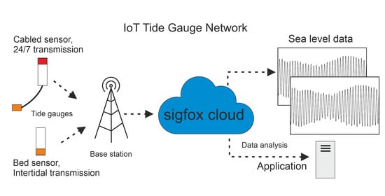
The monitoring system architecture (see Figure 1) comprises a number (depending on the location) of individual tide gauges, all of which communicate with one or more base stations. The base stations then relay the data messages to the “cloud” on a regular basis. Once in the cloud infrastructure, the data can be pushed or picked up by other data servers for postprocessing. For example, the data could consist of 40-s averages of pressure data representing water level, and other statistics of the 10-Hz data, such as burst maximum, minimum and standard deviation, which can be used as a proxy for wave conditions.
The IoT-enabled tide gauge developed here is based on the off-the-shelf Arduino MKR micro-controller. The controller is available with a variety of communications formats, including Sigfox (MKR FOX 1200), LoraWan (MKR WAN 1300), and GSM (MKR GSM 1400). For this project, we chose the MKR FOX 1200 as it has an established subscription-based backend communication infrastructure, and each unit comes with one year’s free subscription. The cost of the MKR FOX 1200 controller is around £40.
The GSM version was excluded because it was twice the price of the others and had relatively high running costs. The LoraWan and Sigfox controllers are very similar in characteristics and cost, but to use the MKR WAN 1300 requires access to a LoraWan base station.
2.2. Arduino Micro-Controller
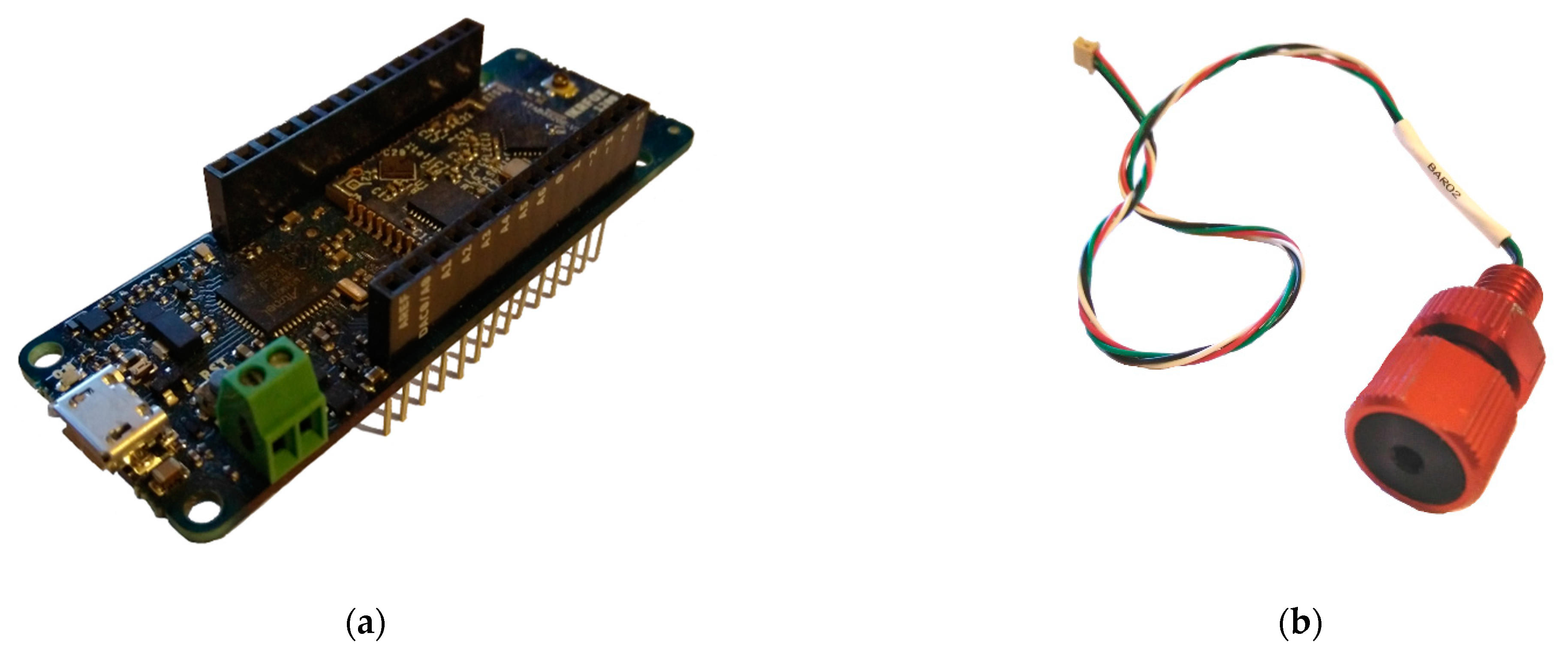
The Arduino MKR FOX 1200 (see Figure 2a) is based on the SAMD21 microchip and an ATA8520 Sigfox module. It has low-power Sigfox communication, 32-bit computational power and can be programmed using the well-supported Arduino Software (IDE) development package.
Power can be supplied via the USB port at 5 V, using a battery pack that does not shut down when the Arduino goes into low-power mode (e.g., the Voltaic Systems USB battery is suitable for this purpose), and at 3.3 V on the I/O pins using a couple of AA, AAA, C or D-cell batteries. The Arduino typically takes around 20 mA, and with the sensors used here and other electronic components, e.g., SD Proto Shield with SD card, gives a total current draw of between 35 and 54 mA, and with a 70 mA current draw during the 1–4 s Sigfox transmission. Bench tests suggest that two alkaline D-cell batteries would last up to 22 days by sampling for 40 s periods and then cycling to sleep mode. Using the Voltaic Systems USB battery with solar panels can allow for continuous recording. The micro-controller is relatively small at 68 mm length and 25 mm width. It is designed to use “prototyping shields” such as the MKR SD Proto Shield, which can be directly plugged in to provide the internal logging option.
2.3. Sigfox Wide-Area Network
The Sigfox module used has a carrier frequency of 868 MHz (working region EU) with an antenna power gain of 2 dB. The Sigfox network permits a maximum of 140 messages of 12 bytes to be sent each day. For instance, the data package could be made up of two integers (taking one byte each) and five floating-point numbers (taking two bytes each). This restriction for the UK is due to European Telecommunications Standards Institute regulations, which only permits devices on these frequencies to send messages 1% of the time (36 s in each hour). The typical communication range is around 10 km in urban areas and 40 km in open countryside.
Data from the IoT devices are delivered to the Sigfox Cloud (see the schematic of the overall network in Figure 1) and redistributed from there to various servers for processing and display. For example, web servers show the tabulated data and graphical outputs; and a computer-server prepares inputs for the waterline algorithms in combination with the marine X-band radar data to produce beach morphology DEMs.
2.4. In-Water Pressure Sensor
A Blue Robotics two-bar pressure and temperature sensor [19] was used for measuring water depths (see Figure 2b). It is based on the Measurement Specialties MS5837 2BA gel-filled, compact, water-resistant sensor [20]. This is a low current (0.6 µA) 24-bit digital output I2C device. The sensor has a quoted 10-bar maximum mechanical pressure, with a standard operating pressure of 0–2 bar, giving an equivalent measuring range of 10 m of seawater (water depth pressure plus atmospheric pressure) with a water depth resolution of 0.16 mm. The Blue Robotics two bar sensor, although relatively expensive at £70 when compared to buying just the pressure sensor (~£4), was chosen for testing since it was already fully waterproof and ready for installation. The pressure sensor was tested in the lab with a 4 m vertical tube of fresh water and performed within ±1 cm when varying the water levels.
2.5. Atmospheric Pressure Sensor
Atmospheric pressure needs to be known when converting the measurements made with the Blue Robotics pressure sensor into the depth of water. The instrument used is a Bosch BME280 environmental sensor, an I2C sensor with temperature, barometric pressure and humidity. It is a low current sensor, 3.6 μA at 1 Hz for humidity, pressure and temperature, and 0.1 μA while in sleep mode.
2.6. Enclosures and Cabling
Various types of enclosures were tested during the field experiments (see Section 3): Experiment 1 used an inexpensive PVC wastewater pipe with waterproof sealed end caps; in Experiment 2, a Blue Robotics 7.62-cm (3-inch) enclosure was used with the standard end caps.
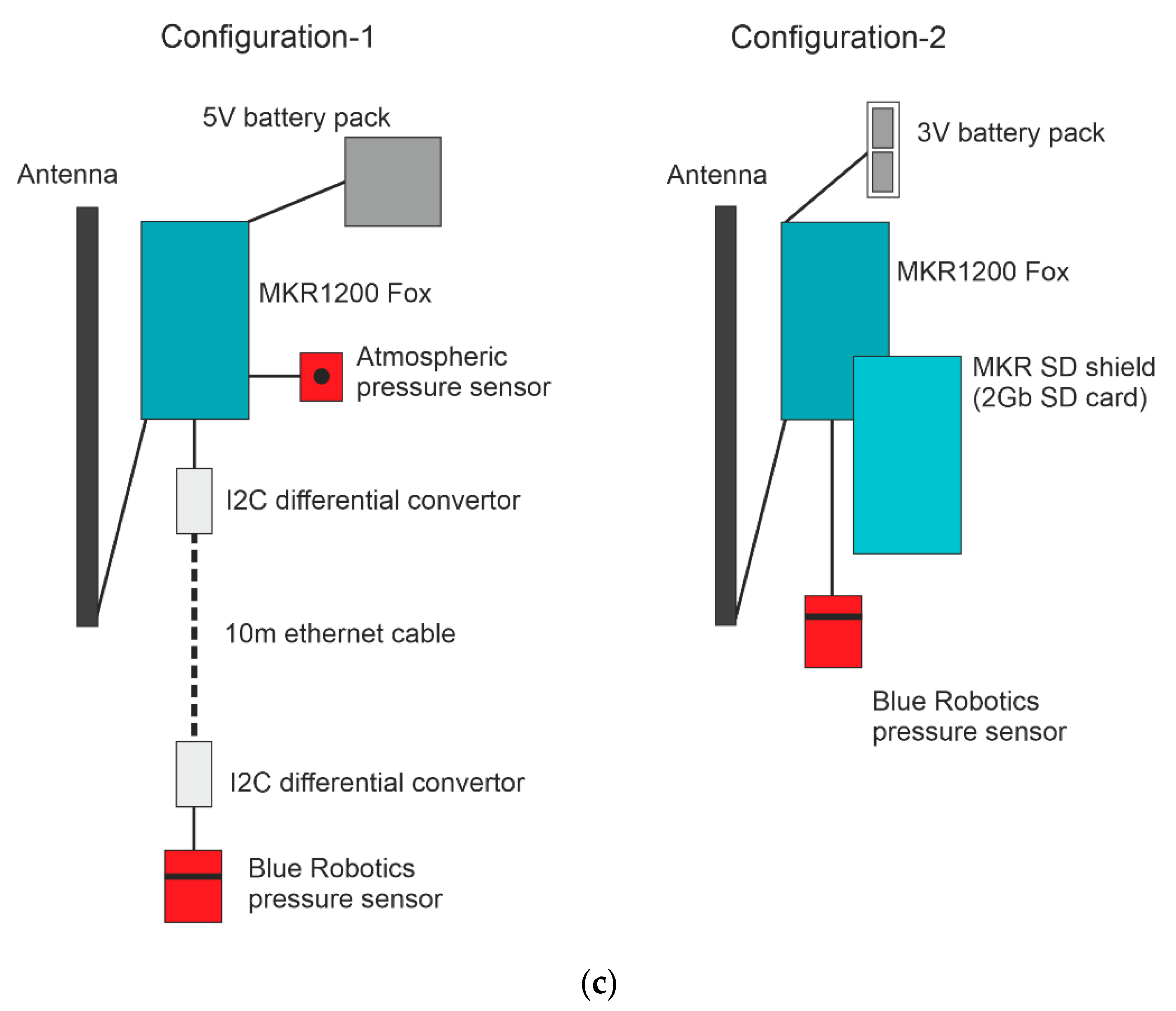
In the first experiment, a PVC pipe (with 5.08 cm (2 inches) diameter and 35 cm length) housed the main electronics and antenna, and a smaller PVC pipe (4 cm diameter with 15 cm length) held the in-water depth pressure sensor and some ancillary components (e.g., an I2C differential converter). The two separate parts were connected using a waterproof ethernet cable that was sealed at both ends using epoxy resin. I2C sensors are limited to using cable lengths of up to one meter; when using much longer cables, such as the 10-m cable (necessary because of the large tidal range), two I2C differential converters must be incorporated at each end of the cable run.
In the second experiment, a Blue Robotics 5.08 cm (2 inches) diameter enclosure contained all the electronic components, antenna and batteries.
2.7. Converting in-Water Pressure Measurements to Water Depth
Using measurements of the water pressure and atmospheric pressure, a water depth can be calculated using the equation:
where water depth is in cm, P is the total pressure at the sensor in millibars, Patm is the atmospheric pressure in millibars, ρ is the density of the seawater in kg m–3, and g is the gravitational acceleration 9.81 m s–2.
water depth = (P − Patm)/(ρ·g)
The main errors in this calculation are associated with determining the seawater density and water temperature. Another uncertainty is introduced because the atmospheric pressure sensor is not located at the same height as the in-water pressure sensor.
3. Field Experiment Locations and Configurations
Experiments were carried out to ascertain the accuracy of the IoT tide gauges compared with established tide gauges and also to demonstrate the versatility of an IoT tide gauge network with its different and complementary hardware and software configurations.
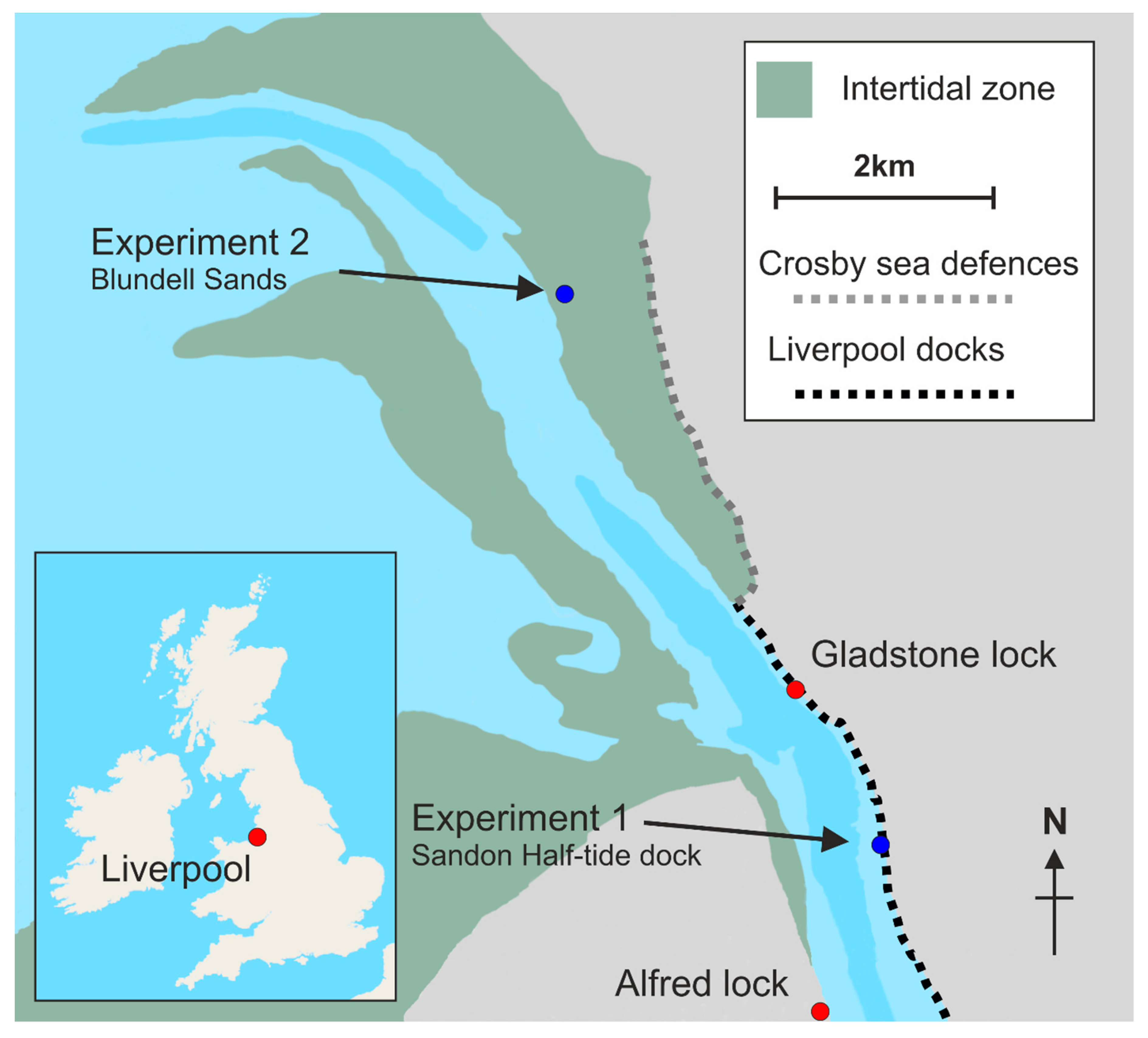
Two different locations were chosen (see Figure 3):
- Experiment 1—a sheltered location beside the dock wall at Liverpool (near to the Sandon Half-tide Dock entrance) on the tidal River Mersey is typical of most tide gauge installations;
- Experiment 2—a beach location at Blundellsands, Crosby, where there is a wide intertidal beach and sea defenses to protect residential areas, with more exposure to waves.
In this macro-tidal region, the tidal range can exceed 10 m at spring tides; at Liverpool, the largest tidal range is 10.35 m, mean high water spring (MHWS) is 9.39 m above local chart datum (CD) while mean low water spring (MLWS) is 1.12 m CD [21]. The local chart datum is 4.93 m below the land-based ordnance datum Newlyn.
3.1. Experiment 1: River Mersey, Liverpool
This site near to the Sandon Half-tide Dock entrance (53°25′37.9″ N, 3°0′22.9″ W, WGS; British National Grid 333,227 392,738) is approximately 2.6 km upstream of the research-quality tide gauge at Gladstone Lock and about 2.6 km downstream of a port authority tide gauge across the river at Alfred Lock (see Figure 3). There are steps down to the water at this location (no public access), and the edge of the river bed is exposed at low water spring tides but not exposed at low water neaps.
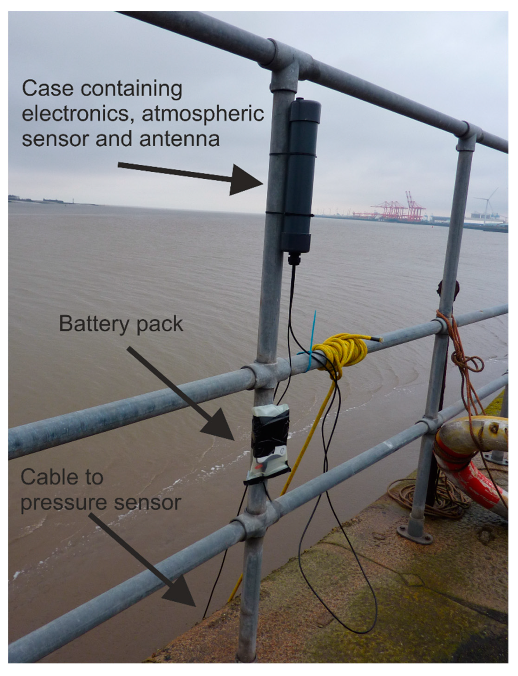
The IoT tide gauge consisted of a Blue Robotics pressure sensor connected by cable to an enclosure containing the Bosch BME 280 sensor, Arduino micro-controller, I2C differential converter and antenna. The enclosure was attached to safety railings on the dock wall along with a separate Voltaic Systems V44 battery (12,000 mAh) (see Figure 4). This battery supports the low-power sleep mode micro-controllers (i.e., it does not turn off if the current draw becomes small during the Arduino’s sleep cycles), and Voltaic Systems solar panels can be added to provide continuous power. A valve was fitted to the top of the enclosure to allow for changes in air pressure. The Blue Robotics pressure sensor was located at the end of an external 10 m long ethernet cable at the bottom of the steps extending down the dock wall, to a couple of meters above the low watermark, in order to capture as much of the tidal range as possible. The installation was leveled to the local vertical datum by measuring the vertical distance from the pressure sensor to the top of the dock wall, the height of which was found using LiDAR data.
Configuration 1 (see Figure 2c) was used for this experiment: set to wake up every 15 min (to be within the 140 daily message limit for Sigfox and to be comparable with the 15 min sampling of the nearby Gladstone lock tide gauge (see Figure 3), record for 40 s (to allow for averaging out of high-frequency wind-generated waves), and then send the averaged pressure and temperature data for each sensor via the Sigfox network. The data package contained the status, BME temperature, BME pressure, BME humidity, Blue Robotics pressure and Blue Robotics temperature. Date/time was added at the Sigfox backend as soon as each message had been received. To save power, no SD card was installed, and hence no data were stored internally during the deployment period.
The IoT tide gauge was deployed for seven days between 1 and 8 November 2019, spanning the transition from spring to neap tides (peak spring tide occurred on 28 October, while lowest neap tide occurred on 6 November).
3.2. Experiment 2: Intertidal Zone, Crosby
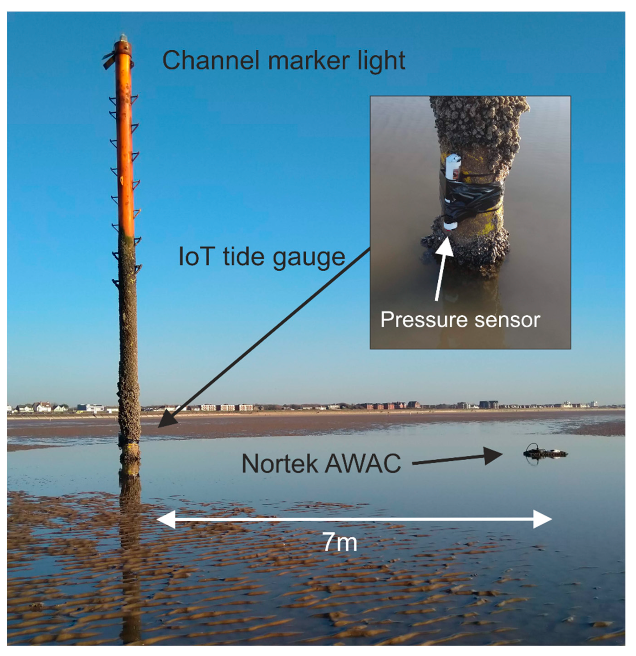
The site on a wide intertidal beach at Blundellsands, Crosby (53°29′43.6″ N, 03°04′1.5″ W, WGS; British National Grid 329306, 400389), is 500 m from the sea defenses and 6 km from Gladstone Lock tide gauge (see Figure 5). The IoT tide gauge was attached to a navigation channel marker post, close to a Nortek acoustic wave and current profiler (AWAC).
The AWAC was part of a local government coastal monitoring study and provided a direct comparison with the measurements from the IoT tide gauge. It was set up to measure currents and sea levels every ten minutes and provide hourly wave measurements based on burst sampling; these data were recovered five months later. The IoT tide gauge was deployed to capture data during Storm Ciara, which arrived in the UK during 8–9 February 2020, to determine the quality of the sea-level data in an exposed intertidal location with expected large waves.
Configuration 2 (see Figure 2c) consisted of Blue Robotics waterproof case enclosing an Arduino micro-controller, MKR SD Proto Shield (with 2 Gb SD card) for storing data, a Blue Robotics pressure sensor with the electronics, two D-cell alkaline batteries and antenna. The Arduino’s internal clock was used for timing, and it was set up to wake up every 15 min, record 40 s of 10-Hz data, calculate maximum, minimum and average values, store these data internally onto the SD card, store the 40-s averages into RAM memory, and send them back via the Sigfox network when the instrument was exposed at low tide (when underwater there was no data transmission). Each data package contained the month, day, hour, minute, and four Blue Robotics pressure values. This configuration allowed most of the sea-level data to be returned during the “dried out” period.
The IoT tide gauge (at the pressure sensor level) and AWAC were leveled to the local vertical datum using heights from GPS. In this experiment, the local atmospheric pressure was obtained from another device at the shoreline (it is envisaged that for an operational IoT tide network that these data would be provided by a weather station colocated with the X-band radar unit or using a cabled configuration as in Section 3.1). The IoT tide gauge was attached to the channel marker (see Figure 5) with cable ties and tape during low water on 6 February and then recovered immediately after the storm; last data were recorded at 00:50 on 10 February.
4. Field Experiment Results
4.1. Comparison of the IoT Tide Gauge and Local Tide Gauges
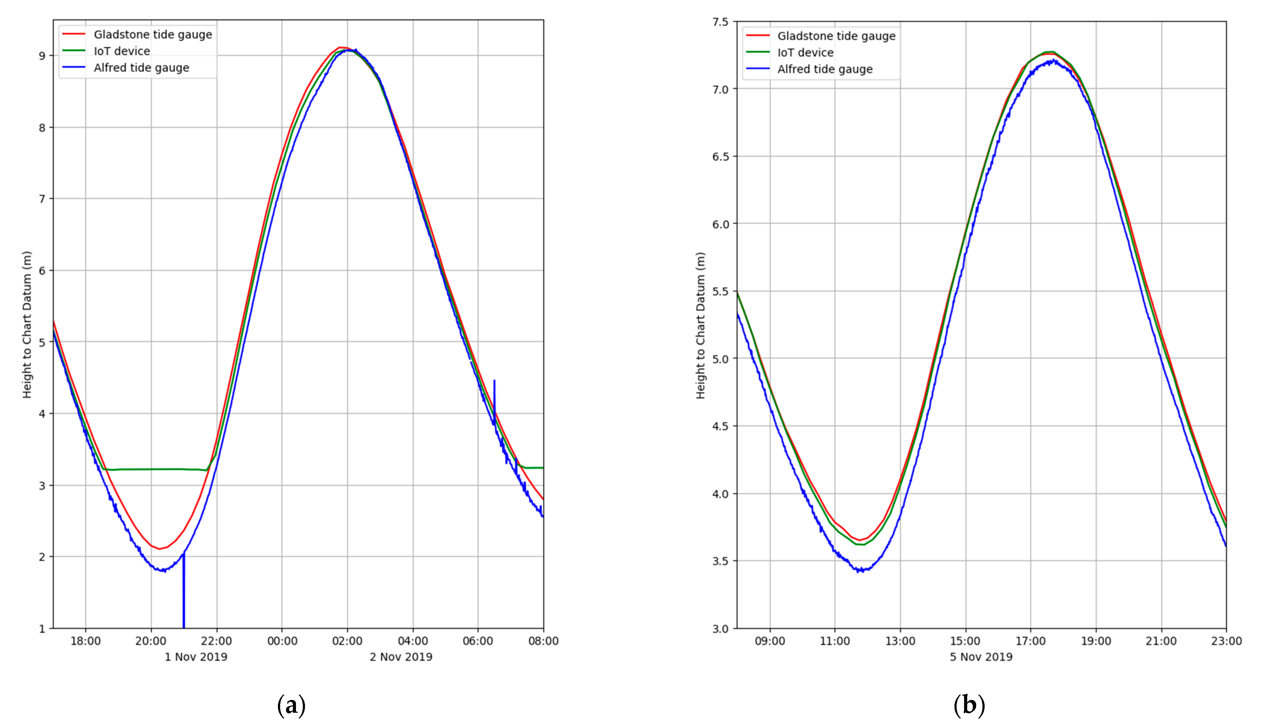
Figure 6a,b compares data from the IoT gauge near Sandon Dock (pressures converted to meters of water) and the local tide gauge records for two periods during the transition from spring to neap tides. Whereas Figure 6c shows the raw pressure data prior to conversion to sea-level values for the whole deployment period. The Gladstone Lock tide gauge records 15-min averages, while the Alfred Lock tide gauge records one-minute averages. At the beginning of the experiment, the tidal range close to the spring tide was large, which exposed the pressure sensor at low water; towards the neap tide, it was always underwater.
The time lags (of a few minutes) in the tidal curves for Gladstone Lock and Alfred Lock reflect their relative locations along the estuary (Figure 6a,b). As the flood tide propagates up the estuary, it reaches Gladstone Lock first, then Sandon Half-tide Dock and Alfred Lock. This can be seen clearly during the approach of high water on 2 November (02:00), with high water at Alfred Lock occurring last. The differences in tidal height and time lag between Sandon Half-tide Dock and Gladstone Lock are smaller than in the corresponding Alfred Lock data, and this is likely because of their locations on the same side of the river/estuary; Figure 3 shows the narrow channel (~940 m at its narrowest part) which connects to an inner much wider part of the estuary (not shown on map), and the corresponding tidal flows are controlled by the cross-section and bed friction [10].
The cabled pressure sensor configuration worked well, giving comparable sea-level data to the established tide gauges and having sent the data successfully via the Sigfox Cloud to the data processing server. The mean difference between the IoT device and the Gladstone lock data was 0.002 m, the standard deviation was 0.035 m, and the root-mean-square difference was 0.035 m (using all the recorded data and ignoring periods when the in-water pressure sensor is exposed to air, i.e., towards low water during Spring tides); the majority of these differences are likely to be due to the 2.6 km separation between locations. The battery pack also worked well; when coupled with solar panels, it would provide continuous power for the IoT tide gauge, necessary for long-term deployments.
4.2. Comparison of the IoT Device and AWAC—Sea Levels
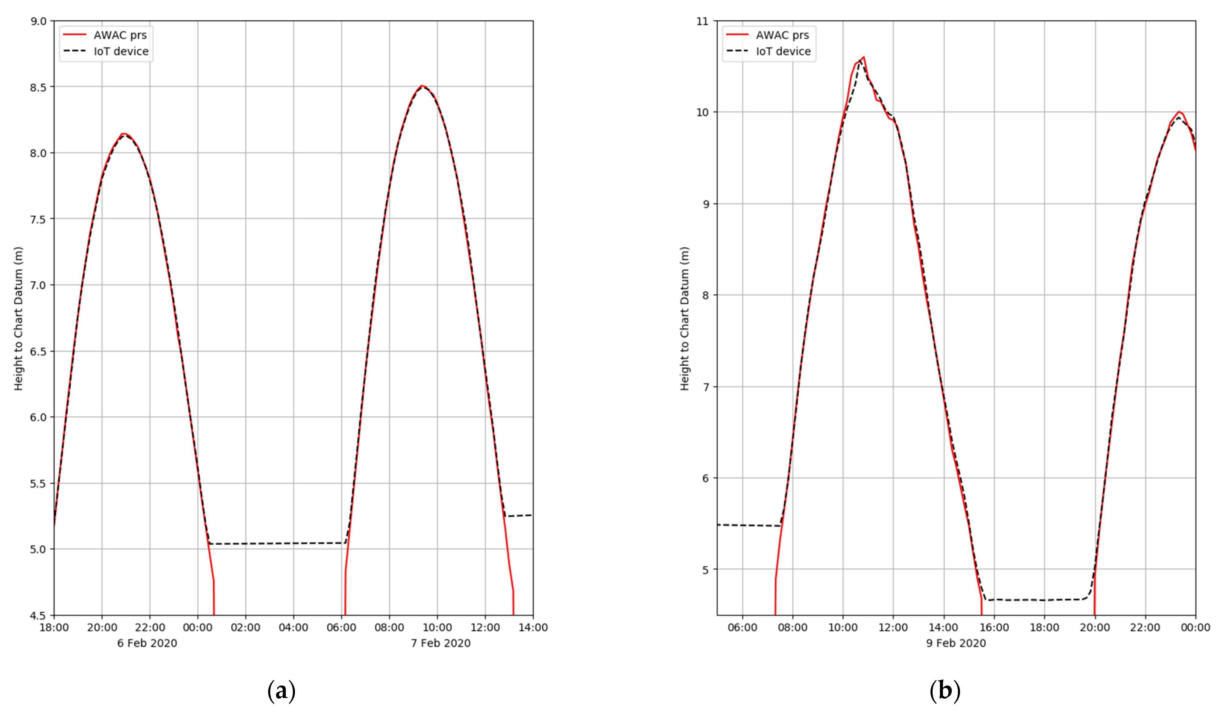
Figure 7 compares sea-level data (with waves minimized by averaging) at Crosby from the IoT device and the AWAC for neap tides between 6 February 18:00 and 7 February 15:00, 2020, and during Storm Ciara on 9 February 05:00–23:59, 2020. The two instruments generally agree during the earlier period (see Figure 7a), but there are obvious differences close to high water during the storm when large waves were present (See Figure 7b). Differences in the last tidal level recorded before drying out and the first tidal level recorded on the flood are an artifact of the rolling 15-min sleep time (sleeps for 15 min, does 40 s measurement and goes to sleep again) and the exact 10-min AWAC data, and combined with the 27-cm vertical separation of the pressure sensors.
The Van de Casteele Test [22] can be applied to determine tide gauge performance. For example, Miguez et al. [23] tested a variety of tide gauges and demonstrated the test’s ability to highlight different types of tide gauge error, while André et al. [24] used it to compare data from three different GNSS buoys for measuring sea level against a nearby radar tide gauge.
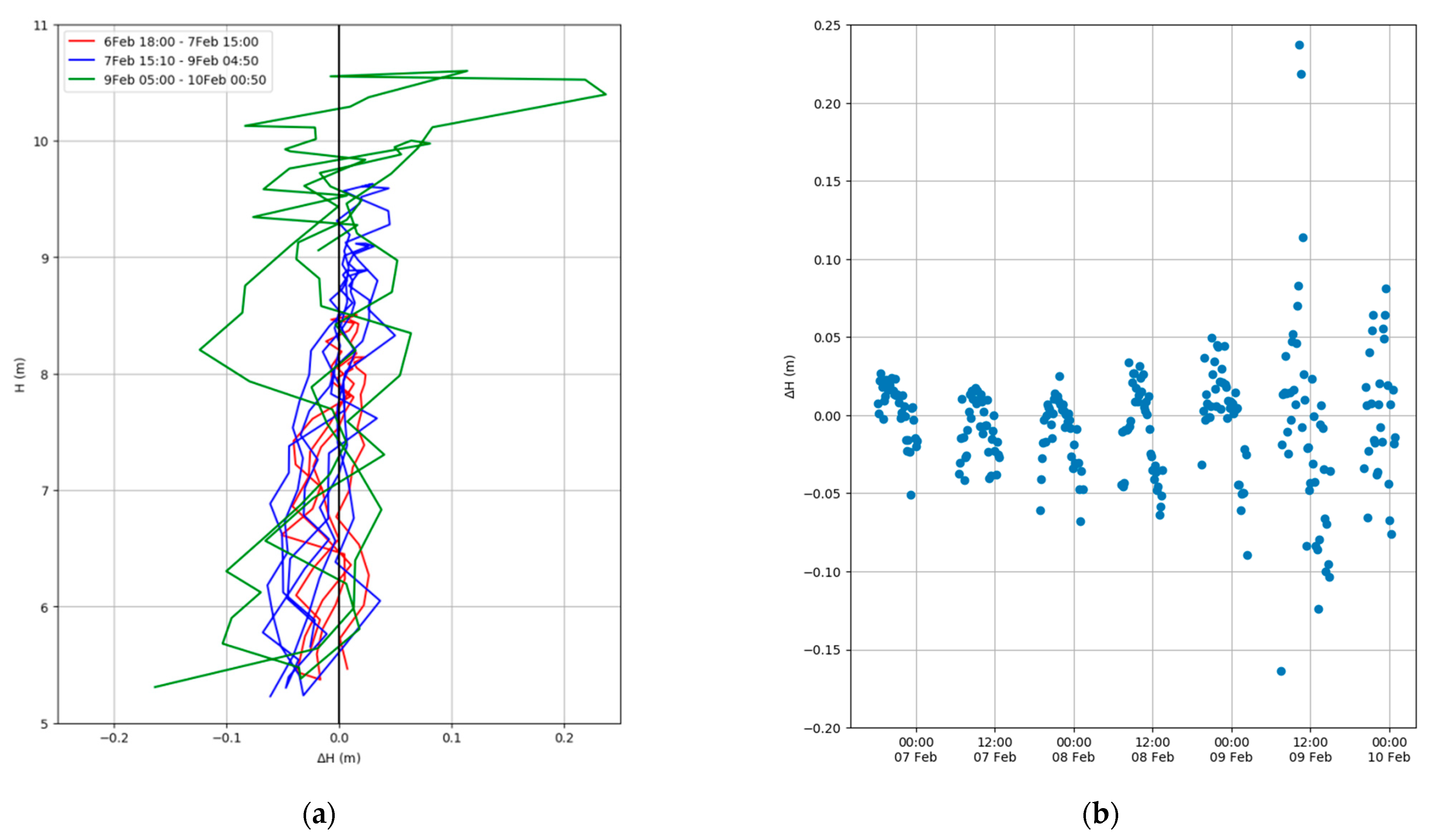
The method compares a reference tide gauge data set (data known to be an accurate measurement of sea level; in this case, the AWAC sea-level data are taken as the reference) to contemporaneous data from the tide gauge being tested (H′): the reference sea-level data (H) are plotted on the ordinate against the tide gauge difference (ΔH) on the abscissa (x-axis), where ΔH = H − H′. The resulting diagram would produce a straight vertical line centered on x = 0 for a perfect match between the two tide gauges.
Applying the Van de Casteele Test to the IoT tide gauge, using the AWAC data as the reference, the near-vertical alignment of the differences in the two data sets (see Figure 8a) between low water and high water, although not perfectly vertical, indicates that there are no timing offsets (which would result in an ellipsoidal pattern) and no obvious systematic errors (such as scale errors, which would introduce a large gradient from low water to high water). The mean difference between the IoT device and the AWAC data was −0.005 m, the standard deviation was 0.040 m, and the root-mean-square difference was 0.040 m (using all the recorded data and ignoring periods when the pressure sensor is exposed to air, i.e., towards low water).
Although there is a slight gradient from low water to high water with larger offsets towards low water, it is unlikely to be due to density differences since both gauges use the same seawater density of 1025 kg m−3 for the conversion to meters of water. However, this small gradient may be a result of turbulence around the channel marker during the lower levels of flood and ebb. Another possible explanation could be air bubbles trapped on the pressure sensor membrane during drying out (this could occur with either pressure sensor); higher pressures towards high water may compress the bubble resulting in smaller pressure differences between them. One way to eliminate this would be to deploy the IoT device horizontally so that the pressure sensor is not facing downwards.
During Storm Ciara, large waves were present, and this can be seen in Figure 7b, Figure 8a,b and Figure 9. The pressure differences (seen within the corresponding sea-levels) become larger with increasing wave heights, and the largest offsets occur between 09:30 and 14:30 on 9 February. These could be caused by the different sampling rates; the IoT device measures for 40 s, and the average is taken for the sea-level measurement, while the AWAC ADCP takes the average over 10 min.
4.3. Comparison of the IoT Device and AWAC—Waves
In Experiment 2, the IoT tide gauge was set up to return sea-level data. However, the recovered data (i.e., 1-Hz data and 40-s period statistics) also demonstrated the capability to capture higher frequency water level variability due to waves. This is explored in this section to illustrate the wider application of the IoT sensor network for monitoring waves.
At this stage, no attempt is made to calculate the pressure attenuation factor, which is necessary to determine actual wave heights in meters of water (this type of processing would be beyond the Arduino micro-controller). However, postprocessing of the internally logged 10-Hz data using open source “R” and Matlab algorithms developed by Miller and Neumeier [25,26] (based on methods outlined by Tucker and Pitt [27]) could be applied to generate the wave height and wave period statistics. For example, Lyman et al. [14] used similar pressure sensors deployed in water depths of 9 m and 18 m and were able to successfully calculate the wave statistics. The AWAC uses a different set of post-recovery algorithms [28] utilizing both the pressure and current to derive the wave statistics.
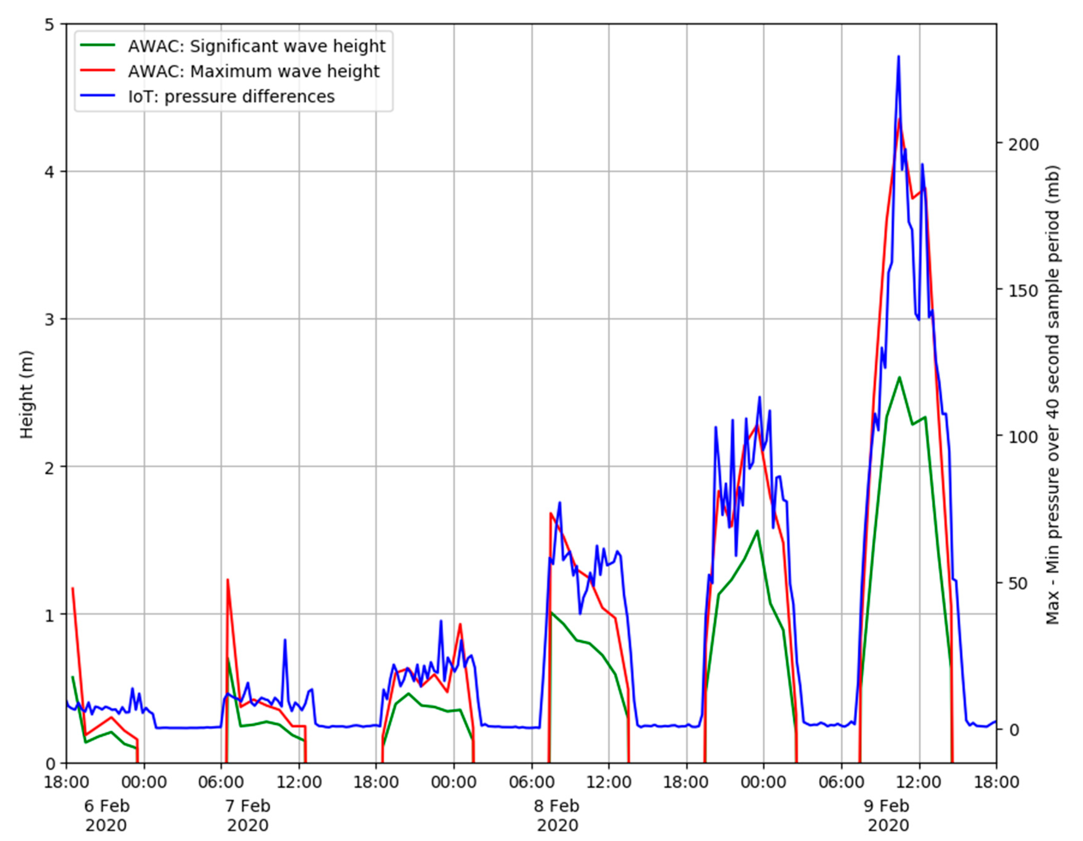
Figure 9 shows the hourly wave statistics from the AWAC, measured during the 1000-s measurement time together with the corresponding differences between maximum and minimum pressure recorded during the 40-s bursts. Although the units of the y-axis scales are different, these IoT pressure statistics do align themselves closely with the maximum wave heights from the AWAC.
It is likely that the IoT pressure sensor is not resolving some of the larger waves since it is only recording for 40 s every 15 min, whereas the AWAC, setup in burst mode to record over 1000 s every hour, can measure the larger waves. While this Configuration 2 did not send these pressure differences via the SigFox network, the software could be modified easily to return them instead. In practice, one IoT tide gauge could send the sea-level data and another the 40-s period burst pressure statistics.
5. Discussion and Conclusions
Experiments 1 and 2 demonstrate the versatility of the Arduino-based devices, with each tide gauge being combined with built-in Sigfox IoT communications and low-cost pressure sensors. While the pressure sensors are capable of measuring sea levels accurately, exposure to waves can contaminate the measurement as the averaged data still appears to contain a contribution from waves, especially during stormy periods. The usual practice is to deploy tide gauges well away from wave exposure. A root-mean-square difference of 0.04 m between the IoT pressure sensor and the AWAC data is an acceptable result, considering the data spanned Storm Ciara. However, deploying the IoT gauge in a more exposed location demonstrates the potential for simultaneously providing valuable information on waves. In addition, the data were successfully transmitted over the Sigfox network and prove that a network of such devices would be feasible. For the proposed tide gauge network, a series of IoT tide gauges based on the Arduino with Sigfox and the pressure sensors would be installed, with a variety of software and hardware configurations.
Experiment 1 using the cabled system was the simplest approach and would be best suited to locations where the antenna (plus electronics) could be in “air” for the deployment period. This type of installation would require a structure such as a pier, breakwater, with either a pole already present or where one could easily be fitted. The navigation pole at the beach location could have been used with this configuration. This hardware with this configuration could be deployed for long periods when combined with solar panels for the battery pack.
The self-contained system used with Experiment 2 demonstrated how the IoT tide gauge would perform if located on a beach with no options for a cabled installation, e.g., attached to the beach with a screw anchor. The inexpensive Blue Robotics enclosure was waterproof and able to withstand the conditions of Storm Ciara; the case was completely watertight even with storm waves impacting it. In this configuration, the IoT device would send back data once the antenna is not underwater and able to transmit. This would allow deployments further offshore nearer to the low water mark and for instrumentation across a wider area of the intertidal zone.
The Van de Casteele test on data from Experiment 2 revealed a small-scale “error” (see small pressure difference gradient in Figure 8a) that may be the result of factors mentioned in Section 4 (bubbles on the pressure sensor membrane may be the main cause of errors). This could be easily verified by testing and deploying the IoT device with the pressure sensor in the horizontal position. The larger pressure differences between the IoT pressure sensor and the AWAC are most likely to have been caused by waves not being filtered out sufficiently by the data-averaging. In addition, the different sampling periods and times of sampling would result in the IoT missing some of the larger waves during its 15-min sleep period. In future experiments, this could be rectified by increasing the 40 s sampling period.
After the success of using off-the-shelf parts for the IoT tide gauge, it would be worthwhile experimenting with lower-powered micro-controllers such as the ATMega 328P driving the same pressure sensors. Lyman et al. [14] have shown that the ATMega 328P is capable of three months of continuous internal logging (to microSD card) of pressures (using MS5803) with three AA batteries and more than a year with D-cell batteries. This would reduce the cost of future devices even more, especially if individual pressure sensors are used (and waterproofed) instead of using the off-the-shelf waterproofed Blue Robotics sensor. In addition, the continuous recording of data would allow for adaptive control to be incorporated into the software, e.g., to send more messages during extreme events.
The two contrasting configurations demonstrate that low-cost IoT tide gauges can provide good quality sea-level data in both real time and “delayed mode” using the Sigfox infrastructure. They can also provide the necessary sea-level data to supplement and enhance coastal monitoring strategies and to support safe port navigation. In addition, the latter configuration also shows the potential to deliver wave information, high-frequency data (after recovery) for post-recovery analysis and the option to transmit proxy wave data in near-real time. Furthermore, the IoT tide gauge network described here could also be used for port operations and to provide ground-truthing for hydrodynamic models of complex locations such as tidal inlets and estuaries.
Author Contributions
P.K. conceived, designed, developed software, performed the experiments, analysed the data and wrote the original draft. A.P. reviewed and edited the final draft. A.P. and J.H. provided supervision. C.B. and A.S. provided project administration and resources. All authors have read and agreed to the published version of the manuscript.
Funding
The research is part of a PhD study funded by the “Low Carbon Eco-Innovatory (LCEI)—Liverpool University” (www.liverpool.ac.uk/environmental-sciences/working-with-business), with industrial partner MM Sensors Ltd.
Institutional Review Board Statement
Not applicable.
Informed Consent Statement
Not applicable.
Data Availability Statement
The data presented in this study are available on request from the author.
Acknowledgments
The authors would like to thank Andrew Martin at Sefton Metropolitan Borough Council for data from the AWAC, Russell Bird at Peel Holdings (Mersey Dock and Harbor Company) for tidal data and access to the docks, and Colin Bell at the National Oceanography Centre for access to the POLTIPS-3 coastal tidal prediction software. The research is part of a PhD study funded by the “Low Carbon Eco-Innovatory (LCEI)—Liverpool University” (www.liverpool.ac.uk/environmental-sciences/working-with-business), with industrial partner MM Sensors Ltd. This paper contributes to Work Package 4 of the UK NERC-funded BLUEcoast project (NE/N015614/1).
Conflicts of Interest
The authors declare no conflict of interest.
References
- Scott, T.; Masselink, G.; O’Hare, T.; Saulter, A.; Poate, T.; Russell, P.; Davidson, M.; Conley, D. The extreme 2013/2014 winter storms: Beach recovery along the southwest coast of England. Mar. Geol. 2016, 382, 224–241. [Google Scholar] [CrossRef] [Green Version]
- Hanley, M.; Hoggart, S.; Simmonds, D.; Bichot, A.; Colangelo, M.; Bozzeda, F.; Heurtefeux, H.; Ondiviela, B.; Ostrowski, R.; Recio, M. Shifting sands? Coastal protection by sand banks, beaches and dunes. Coast. Eng. 2014, 87, 136–146. [Google Scholar] [CrossRef]
- Walvin, S.; Mickovski, S. A comparative study of beach nourishment methods in selected areas of the coasts of the United Kingdom and The Netherlands. WIT Trans. Built Environ. 2015, 148, 85–96. [Google Scholar]
- Russell, P.E. Mechanisms for beach erosion during storms. Cont. Shelf Res. 1993, 13, 1243–1265. [Google Scholar] [CrossRef]
- Klemas, V. Beach profiling and LIDAR bathymetry: An overview with case studies. J. Coast. Res. 2011, 27, 1019–1028. [Google Scholar] [CrossRef]
- Bell, P.S.; Bird, C.O.; Plater, A.J. A temporal waterline approach to mapping intertidal areas using X-band marine radar. Coast. Eng. 2016, 107, 84–101. [Google Scholar] [CrossRef] [Green Version]
- Elko, N.; Briggs, T.R.; Benedet, L.; Robertson, Q.; Thomson, G.; Webb, B.M.; Garvey, K. A century of US beach nourishment. Ocean Coast. Manag. 2021, 199, 105406. [Google Scholar] [CrossRef]
- Metters, D.; Shayer, J.; Ryan, J.; Bourner, J.; Corbett, B.; Tomlinson, R. Strategic and cost-effective networks of miniaturised tide gauges. In Proceedings of the Australasian Coasts & Ports 2017: Working with Nature, Cairns, Australia, 21–23 June 2017; p. 965. [Google Scholar]
- Joseph, A.; Prabhudesai, R. Web-enabled and real-time reporting: Cellular based instrumentation for coastal sea level and surge monitoring. In The Indian Ocean Tsunami; CRC Press: Boca Raton, FL, USA, 2006; pp. 247–257. [Google Scholar]
- Pugh, D.; Woodworth, P. Sea-Level Science: Understanding Tides, Surges, Tsunamis and Mean Sea-Level Changes; Cambridge University Press: Cambridge, CA, USA, 2014. [Google Scholar]
- Williams, S.D.; Bell, P.S.; McCann, D.L.; Cooke, R.; Sams, C. Demonstrating the Potential of Low-Cost GPS Units for the Remote Measurement of Tides and Water Levels Using Interferometric Reflectometry. J. Atmos. Ocean. Technol. 2020, 37, 1925–1935. [Google Scholar] [CrossRef]
- Knight, P.J.; Bird, C.O.; Sinclair, A.; Plater, A.J. A low-cost GNSS buoy platform for measuring coastal sea levels. Ocean Eng. 2020, 203, 107198. [Google Scholar] [CrossRef]
- Beddows, P.A.; Mallon, E.K. Cave pearl data logger: A flexible Arduino-based logging platform for long-Term monitoring in harsh environments. Sensors 2018, 18, 530. [Google Scholar] [CrossRef] [PubMed] [Green Version]
- Lyman, T.P.; Elsmore, K.; Gaylord, B.; Byrnes, J.E.; Miller, L.P. Open Wave Height Logger: An open source pressure sensor data logger for wave measurement. Limnol. Oceanogr. Methods 2020, 18, 335–345. [Google Scholar] [CrossRef]
- Holgate, S.; Foden, P.; Pugh, J.; Woodworth, P. Real time sea level data transmission from tide gauges for tsunami monitoring and long term sea level rise observations. J. Oper. Oceanogr. 2008, 1, 3–8. [Google Scholar] [CrossRef] [Green Version]
- Pérez, B.; Álvarez Fanjul, E.; Pérez, S.; de Alfonso, M.; Vela, J. Use of tide gauge data in operational oceanography and sea level hazard warning systems. J. Oper. Oceanogr. 2013, 6, 1–18. [Google Scholar] [CrossRef]
- Kim, T.-H.; Ramos, C.; Mohammed, S. Smart city and IoT. Future Gener. Comput. Syst. 2017, 76, 159–162. [Google Scholar] [CrossRef]
- Bresnahan, P.J.; Wirth, T.; Martz, T.; Shipley, K.; Rowley, V.; Anderson, C.; Grimm, T. Equipping smart coasts with marine water quality IoT sensors. Results Eng. 2020, 5, 100087. [Google Scholar] [CrossRef]
- Blue Robotics Bar02 Ultra High Resolution 10 m Depth/Pressure Sensor. Available online: https://bluerobotics.com/store/sensors-sonars-cameras/sensors/bar02-sensor-r1-rp/ (accessed on 1 November 2020).
- Measurement Specialties, MS5837-02BA Data Sheet. Available online: https://www.te.com/commerce/DocumentDelivery/DDEController?Action=srchrtrv&DocNm=MS5837-02BA01&DocType=Data+Sheet&DocLang=English&DocFormat=pdf&PartCntxt=CAT-BLPS0059 (accessed on 6 December 2020).
- National Oceanography Centre. National Tidal & Sea Level Facility: Liverpool Tide Gauge Statistics. Available online: https://www.ntslf.org/tgi/portinfo?port=Liverpool (accessed on 10 September 2020).
- Miguez, B.M.; Testut, L.; Wöppelmann, G. The Van de Casteele test revisited: An efficient approach to tide gauge error characterization. J. Atmos. Ocean. Technol. 2008, 25, 1238–1244. [Google Scholar] [CrossRef]
- Míguez, B.M.; Testut, L.; Wöppelmann, G. Performance of modern tide gauges: Towards mm-level accuracy. Sci. Mar. 2012, 76, 221–228. [Google Scholar] [CrossRef]
- André, G.; Míguez, B.M.; Ballu, V.; Testut, L.; Wöppelmann, G. Measuring sea level with GPS-equipped buoys: A multi-instruments experiment at Aix Island. Int. Hydrogr. Rev. 2013, 10, 27–38. [Google Scholar]
- Miller, L.P.; Neumeier, U. Oceanwaves: Ocean Wave Statistics (R). Available online: https://cran.r-project.org/web/packages/oceanwaves/index.html (accessed on 15 November 2020).
- Neumeier, U. Oceanwaves: Ocean Wave Statistics (Matlab). Available online: http://neumeier.perso.ch/matlab/waves.html (accessed on 15 November 2020).
- Tucker, M.J.; Pitt, E.G. Waves in Ocean Engineering; Elsvier: Amsterdam, The Netherlands, 2001. [Google Scholar]
- Nortek Manuals. Available online: https://support.nortekgroup.com/hc/en-us/categories/360001447411-Manuals (accessed on 15 November 2020).
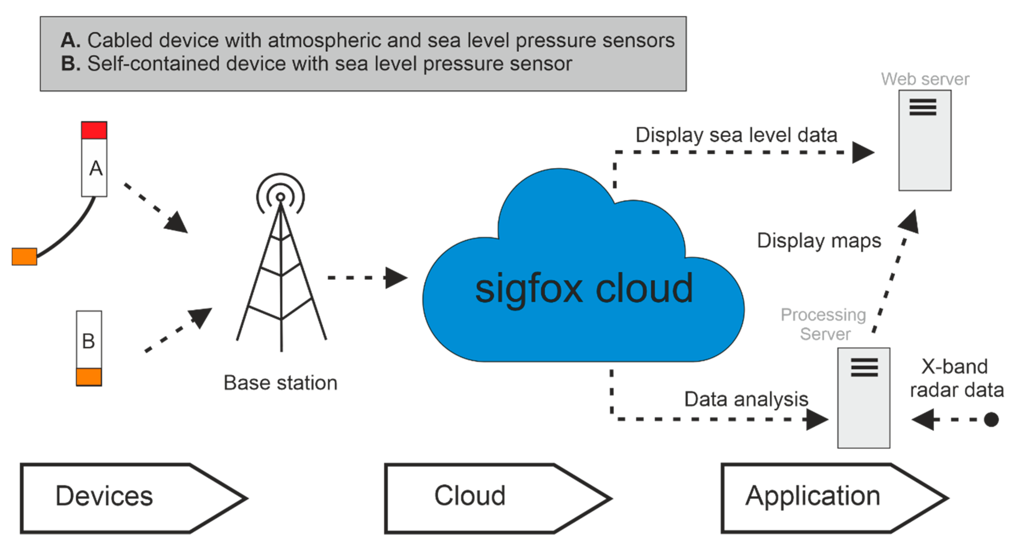
Figure 1.
Monitoring system architecture.

Figure 2.
(a) Arduino MKR 1200 Fox micro-controller, (b) Blue Robotics 2-bar (MS5837 pressure sensor), (c) Configuration-1 and Configuration-2.
Figure 2.
(a) Arduino MKR 1200 Fox micro-controller, (b) Blue Robotics 2-bar (MS5837 pressure sensor), (c) Configuration-1 and Configuration-2.


Figure 3.
Fieldwork and local tide gauge locations in the Mersey Estuary; local tide gauges (red dots), experiments (blue dots).
Figure 3.
Fieldwork and local tide gauge locations in the Mersey Estuary; local tide gauges (red dots), experiments (blue dots).

Figure 4.
Sensor installation at Sandon Half-tide dock, Liverpool.

Figure 5.
Sensor installation at Crosby (Blundellsands). The “Internet of Things” (IoT) tide gauge was attached to the channel marker, and the Nortek acoustic wave and current profiler (AWAC) was located 7 m away and attached with a chain.
Figure 5.
Sensor installation at Crosby (Blundellsands). The “Internet of Things” (IoT) tide gauge was attached to the channel marker, and the Nortek acoustic wave and current profiler (AWAC) was located 7 m away and attached with a chain.

Figure 6.
Liverpool tidal elevations (Gladstone Lock—red, IoT device—green, Alfred Lock—blue), (a) Spring period: 1 November 17:00–2 November 08:00, 2019, (b) Neap period: 5 November 08:00–23:00, 2019, (c) raw in-water pressures from the Blue Robotics pressure sensor for the whole deployment period.


Figure 7.
Crosby tidal elevations (AWAC—red line, IoT tide gauge—black dashed line), (a) neap tides: 6 February 18:00–7 February 15:00, 2020, (b) Storm Ciara: 9 February 05:00–23:59, 2020.
Figure 7.
Crosby tidal elevations (AWAC—red line, IoT tide gauge—black dashed line), (a) neap tides: 6 February 18:00–7 February 15:00, 2020, (b) Storm Ciara: 9 February 05:00–23:59, 2020.

Figure 8.
Results of the Van de Casteele test: (a) for the IoT tide gauge using the AWAC tide gauge as a reference. (b) Time-series of tide gauge differences.
Figure 8.
Results of the Van de Casteele test: (a) for the IoT tide gauge using the AWAC tide gauge as a reference. (b) Time-series of tide gauge differences.

Figure 9.
Time-series comparisons left y-axis: significant and maximum wave heights from the AWAC ADCP right y-axis: differences between maximum and minimum pressures recorded during the 40-s burst.
Figure 9.
Time-series comparisons left y-axis: significant and maximum wave heights from the AWAC ADCP right y-axis: differences between maximum and minimum pressures recorded during the 40-s burst.

Publisher’s Note: MDPI stays neutral with regard to jurisdictional claims in published maps and institutional affiliations. |
© 2021 by the authors. Licensee MDPI, Basel, Switzerland. This article is an open access article distributed under the terms and conditions of the Creative Commons Attribution (CC BY) license (http://creativecommons.org/licenses/by/4.0/).
Share and Cite
MDPI and ACS Style
Knight, P.; Bird, C.; Sinclair, A.; Higham, J.; Plater, A. Testing an “IoT” Tide Gauge Network for Coastal Monitoring. IoT 2021, 2, 17-32. https://doi.org/10.3390/iot2010002
AMA Style
Knight P, Bird C, Sinclair A, Higham J, Plater A. Testing an “IoT” Tide Gauge Network for Coastal Monitoring. IoT. 2021; 2(1):17-32. https://doi.org/10.3390/iot2010002
Chicago/Turabian StyleKnight, Philip, Cai Bird, Alex Sinclair, Jonathan Higham, and Andy Plater. 2021. "Testing an “IoT” Tide Gauge Network for Coastal Monitoring" IoT 2, no. 1: 17-32. https://doi.org/10.3390/iot2010002