
A Hidden Markov Model and Fuzzy Logic Forecasting Approach for Solar Geyser Water Heating


1
iDigi-Tech, First National Bank, Gauteng, Randburg 2194, South Africa
2
Department of Electrical, Electronic and Computer Engineering, Central University of Technology, Centre for Sustainable Smart Cities, Free State, Private Bag X20539, Bloemfontein 9300, South Africa
3
Information Technology Group, Wageningen University and Research, Leeuwenborch, Hollandseweg 1, 6706 KN Wageningen, The Netherlands
*
Author to whom correspondence should be addressed.
Infrastructures 2021, 6(5), 67; https://doi.org/10.3390/infrastructures6050067
Submission received: 4 March 2021
/
Revised: 16 April 2021
/
Accepted: 22 April 2021
/
Published: 30 April 2021
(This article belongs to the Special Issue Investigating Waste Behaviours for Reducing the Strain on Critical Infrastructures)
Abstract
:Time-based smart home controllers govern their environment with a predefined routine, without knowing if this is the most efficient way. Finding a suitable model to predict energy consumption could prove to be an optimal method to manage the electricity usage. The work presented in this paper outlines the development of a prediction model that controls electricity consumption in a home, adapting to external environmental conditions and occupation. A backup geyser element in a solar geyser solution is identified as a metric for more efficient control than a time-based controller. The system is able to record multiple remote sensor readings from Internet of Things devices, built and based on an ESP8266 microcontroller, to a central SQL database that includes the hot water usage and heating patterns. Official weather predictions replace physical sensors, to provide the data for the environmental conditions. Fuzzification categorises the warm water usage from the multiple sensor recordings into four linguistic terms (None, Low, Medium and High). Partitioning clustering determines the relationship patterns between weather predictions and solar heating efficiency. Next, a hidden Markov model predicts solar heating efficiency, with the Viterbi algorithm calculating the geyser heating predictions, and the Baum–Welch algorithm for training the system. Warm water usage and solar heating efficiency predictions are used to calculate the optimal time periods to heat the water through electrical energy. Simulations with historical data are used for the evaluation and validation of the approach, by comparing the algorithm efficiency against time-based heating. In a simulation, the intelligent controller is 19.9% more efficient than a time-based controller, with higher warm water temperatures during the day. Furthermore, it is demonstrated that a controller, with knowledge of external conditions, can be switched on 728 times less than a time-based controller.
1. Introduction
Time-based smart home controllers maintain the temperature of their environment by adopting the use of a predefined routine. However, this is an inefficient process as the controller activates or deactivates specific applications based on a trigger or time. It does not alter its predefined algorithm to support changes in surrounding conditions. Finding a suitable prediction model to predict energy consumption is a significantly more efficient way in which to control electricity usage. There is also a need to have a model that is able to adapt to external environmental conditions, occupations and human behavioural patterns. Yet, modelling human behaviour is challenging in particular, due to the unpredictable nature of human actions. The study of circadian rhythm is the investigation of behavioural changes in a human when responding to the solar cycles of light and darkness; where activities are synchronized around a biological clock that requires light to reset each morning [1]. Medical research has demonstrating that the master circadian clock in humans is the superchiasmatic nuclei (SCN) and ensures that individuals remain in sync with the external world. Therefore, based on an understanding on of the SCN, it is possible to predict and model general human periods of activity [2]. This prediction information is ideal for developing more detailed energy consumption models that cater for the creation of smart home heating systems. In this paper, the focuses are specifically on the development of a suitable model to predict energy consumption of solar geyser water heating, which is able to adapt to external environmental conditions and warm water usage. The system that forecasts warm water usage and solar efficiency (and controls the standby electrical element) more efficiently than time-base controllers.
The research methodology investigates a suitable machine learning algorithm to forecast solar geyser warm water heating. Specifically, the hidden Markov model (HMM) with fuzzy logic is used to forecast the water consumption trends and solar efficiency levels. The contribution of this study involves altering the Baum–Welch algorithm, at the HMM training stage in order to decrease the observation sequence, makes the model more reactive to sudden weather changes and increasing the efficiency of the prediction model. The remainder of this paper is as follows: Section 2 discussed the background and related work. The system methodology is presented in Section 3 and the Data Collection and Implementation is clarified in Section 4. The Results are presented in Section 5 and the paper is concluded in Section 6.
2. Background
Time-based smart home controllers maintain their environment inefficient by adopting the use of a predefined routine. Finding a suitable prediction model, that supports changes in surrounding conditions, to predict energy consumption is a significantly more efficient way in which to control electricity usage. Energy efficiency and smart heating systems are becoming an increasingly in demand technology as urbanisation increases. There is a need for energy, water and food provision to become smarter, more technologically driven and less wasteful. Many works have investigated the use of Industry 4.0 technologies as a solution for this. For example, Dintchev et al. [3], indicate that in summer periods, the performance of the studied solar geyser is very satisfactory, and the electrical backup element active time is minimal. It is recommended that, in the summer period, the electrical element is switched off during the day for maximum solar heating benefits but switched on when it is dark or when it is cloudy and rainy. During the winter months, the solar heating is reduced by 70% and the backup element should be controlled by a controller all the time. Similarly, this research is confirmed by Sauer et al., who employ clustering and hidden Markov models to determine the levels of solar radiation for a specific location from temperature, sky coverage and the previous years’ radiation from a national database. Whereas, Delport et al. [4] indicated that the geyser losses in winter is higher than in summer and the use of hot water in winter is higher than in summer [5]. LaMeres et al. [6] presented a fuzzy logic variable power control strategy, where the geyser element power consumption is controlled, based on information available such as water temperature, minimum and maximum water temperatures allowed and the distribution level power demand to improve the load factor of residential load profiles. Catherine et al. [7] researched the efficiency of a geyser management system through intelligent hot water usage profiling. Bakker et al. [8] presented the use of artificial neural networks with the previous day and previous week heat demand profile to predict the following twenty-four-hour heat demand of individual households.
Saving power consumption can also been achieved by altering the design of the element. A review written by Hohne et al. [9] indicated that by replacing one 4 kW element with two 2 kW elements, and each element is controlled by its own thermostat (but one is set 5 °C lower), can reduce the total energy used to heat the water, as now with small water usage, only one element is switched on to reheat. With a single element, it is found that the system overheats by average of 4 °C. With the dual element the temperature is regulated near the set point and overheating temperatures are halved. Another geyser design changed is researched by Thomas et al. [10], where the hot water is monitored at different levels in a geyser as cold water remains at the bottom of the cylinder because it is denser than hot water. The bottom temperature will drop first and by rising the thermostat will decrease the amount of times that the element is activated to heat up the water. A notable consideration is to ensure that the geyser water is not below 45 °C for significant periods, as heating water with a solar radiation without electrical backup during inefficient cycles is dangerous due to a disease known as Legionellosis. Wolter et al. [11] researched legionnaires disease in South Africa and confirmed it is caused by a bacterium known as Legionella pneumophila responsible for several fatalities worldwide. Suitable growing conditions for the bacteria is between 20 °C and 45 °C. The bacteria die within 5 to 6 h at 55 °C, 32 min at 60 °C and at temperatures above 70 °C the bacteria are killed immediately [12]. Based on this assessment, the following section proposes a methodology for the intelligent measure and control of electricity usage in a home environment.
3. Methodology
In this section, the implementation of hardware for measurement, control and communication is discussed. Figure 1a illustrates a block diagram of the controller that analyses and records all input data. The recorded data is stored in an SQL database. The data is analysed with partial clustering to identify specific patterns. The prediction model formulated is a combination of fuzzy logic with hidden Markov model forecast the following twenty-four hours consumption and solar efficiency. Based on the prediction, the model controls the output actuator that are a geyser’s electrical element. Figure 1b illustrates a basic layout between the controller and the IoT devices. The IoT devices can be a Wi-Fi device with multiple input sensors and output actuators or can also be internet-based, like weather predictions or a user controlling the setup via a web page. The device caters for any combination of sensors and they do not need to be of the same type for example control geyser and room light from the same IoT device.
3.1. Hardware Setup
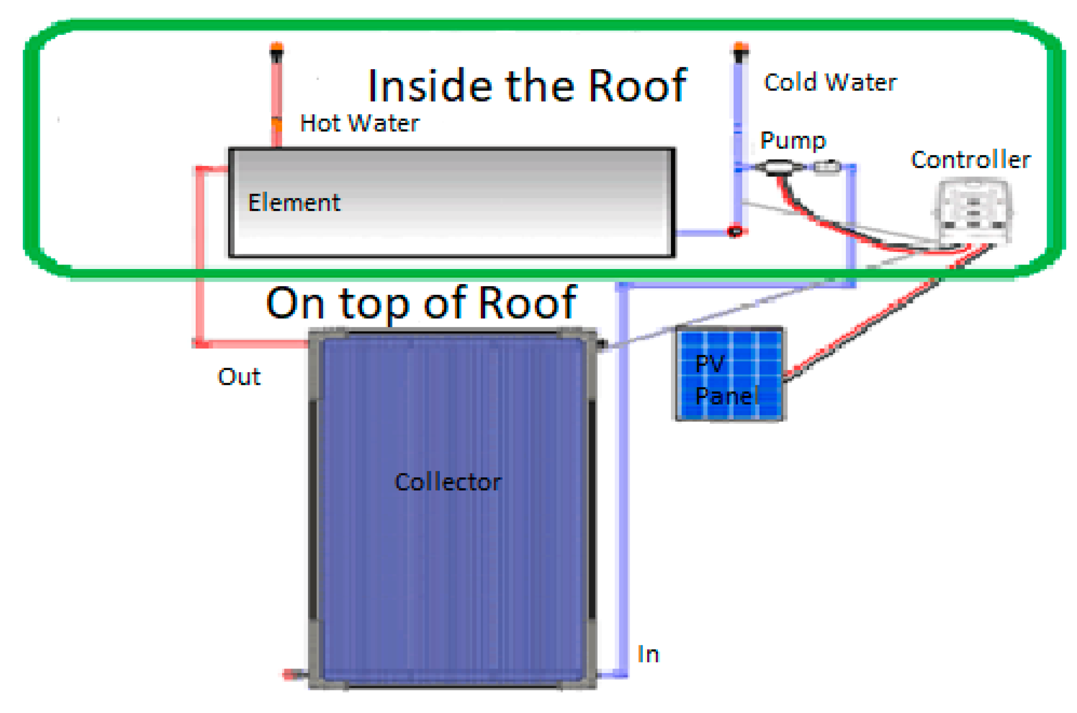
The research is conducted in Johannesburg South Africa, which lays in the summer rainfall region. The system is installed in a residential house, which is occupied by four people busy with their daily routines, which include going to work or school. The hardware setup involves a 200-litre electrical geyser, with a 4 kW element, controlled with a time-based controller [13]. The geyser is also connected to an outside solar water collector with a solar pump. The pump is connected to an external photovoltaic (PV) panel, controlling the circulation of the water through the geyser if the outside panel water temperature is 7 °C higher than inside the geyser as illustrated in Figure 2.
The requirement for the recording device is to record warm water usage, solar heating and standby electrical heating. This requires temperature sensors recording the geyser water temperature, warm water pipe temperature and temperature inside the roof. The ambient roof temperature is needed for calculating geyser heat losses and is presented in Equation (1) [14].
where, qloses is the heat loss in W/m2, Th is the water temperature inside the Hot Water Cylinder (HWC) and Tambient is the air temperature outside the HWC in °C, Δx is the thickness of insulation in m, k is the thermal conductivity in W/m·K and h is the surface heat transfer coefficient in W/m2·K.
The devices utilizing electricity also require current sensor recording when an electrical element is switched on, and movement sensors recorded occupation. This requires the use of IoT-ready technologies. Multiple off-the-shelf home controlling systems were investigated for this, but none were found to be suitable, as access to recorded data is required. Therefore, a bespoke setup is employed and Table 1 indicates the specification of the components used for the IoT sensor set up.
The ESP8266-12E monitors the geyser element with a sealed electromagnetic H105F-1 SPST relay providing a maximum contact current of 40A and average resistive load of 30A@240V AC. Recording the temperatures is done with three LM317 temperature sensors. The completed recording device is illustrated in Figure 3.
3.2. Sensor Registration
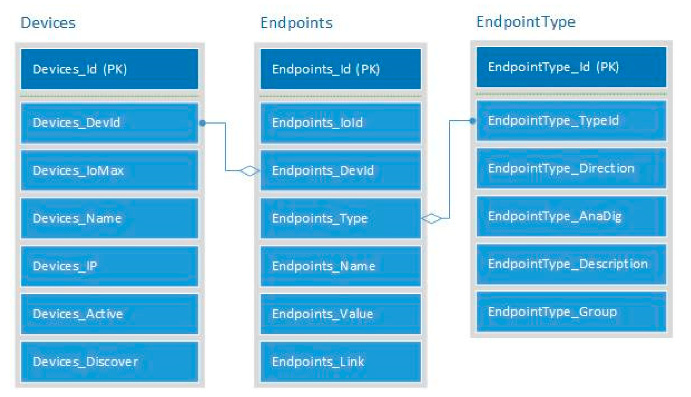
The software is implemented in Microsoft Visual Basic Studio 2010 and SQL 2010 on a Microsoft Windows 10 operation system to receive and store data from multiple devices with multiple sensors. The device must be able to be software defined for multiple applications and the General Purpose Input/Output (GPIO) pin’s including its feature must be registered as an endpoint when the sensor registers with the controller. This scalable design enables the controller to add any future type sensor as illustrated in Table 2. Figure 4 illustrates the SQL table structure created to support sensor registration and value recording. When the ESP8266 registers, it requires a unique identification. The device ID, amount of IO’s, name and IP address are registered. The controller then requests the information of each endpoint. The endpoint ID, with the devices ID, endpoint type and endpoint name are stored in the endpoints table. The value of the endpoint is requested, after the controller associated an endpoint with an application feature.
The IoT sensors update the server whenever any sensor reading changes. The server saves all this information into the SQL database to be analysed later.
3.3. Process Overview
An overview of the three-stage process is as follows.
(1) profiling geyser water usage, which involves (a) fuzzified roof temperature, warm water pipe temperature and geyser water temperature into crisp warm water usages: None, Small, Medium and Large (Algorithm 1).
| Algorithm 1: Fuzzified geyser, roof and pipe temperatures |
 |
(2) profiling solar geyser efficiency, concerning (a) analysis roof temperature, warm water pipe temperature and geyser water temperature and weather conditions—temperature, humidity, wind speed and cloud cover with partial partitioning seeking for the relationship between environmental conditions and the solar heating efficiency; (b) based on partial partitioning the HMM created for rainy season: None, Low and High; (c) Viterbi algorithm used to predict solar geyser efficiency; (d) modified Baum–Welch algorithm with forward (example 1) and backwards (example 2) algorithm used to train the model (Algorithms 2 and 3).
| Algorithm 2: Baum–Welch algorithm modification 1 |
 |
| Algorithm 3: Baum–Welch algorithm |
 |
 |
(3) combining warm water usage prediction and solar efficiency prediction calculating optimal periods enabling electrical standby element (Algorithms 4 and 5).
| Algorithm 4: Calculate to enable geyser element |
 |
| Algorithm 5: Final prediction to enable geyser element |
 |
4. Data Analysis
Following the methodology outlined previously, this section discusses the process for profiling the geyser’s warm water usages and solar heating.
4.1. Fuzzified Geyser Usages
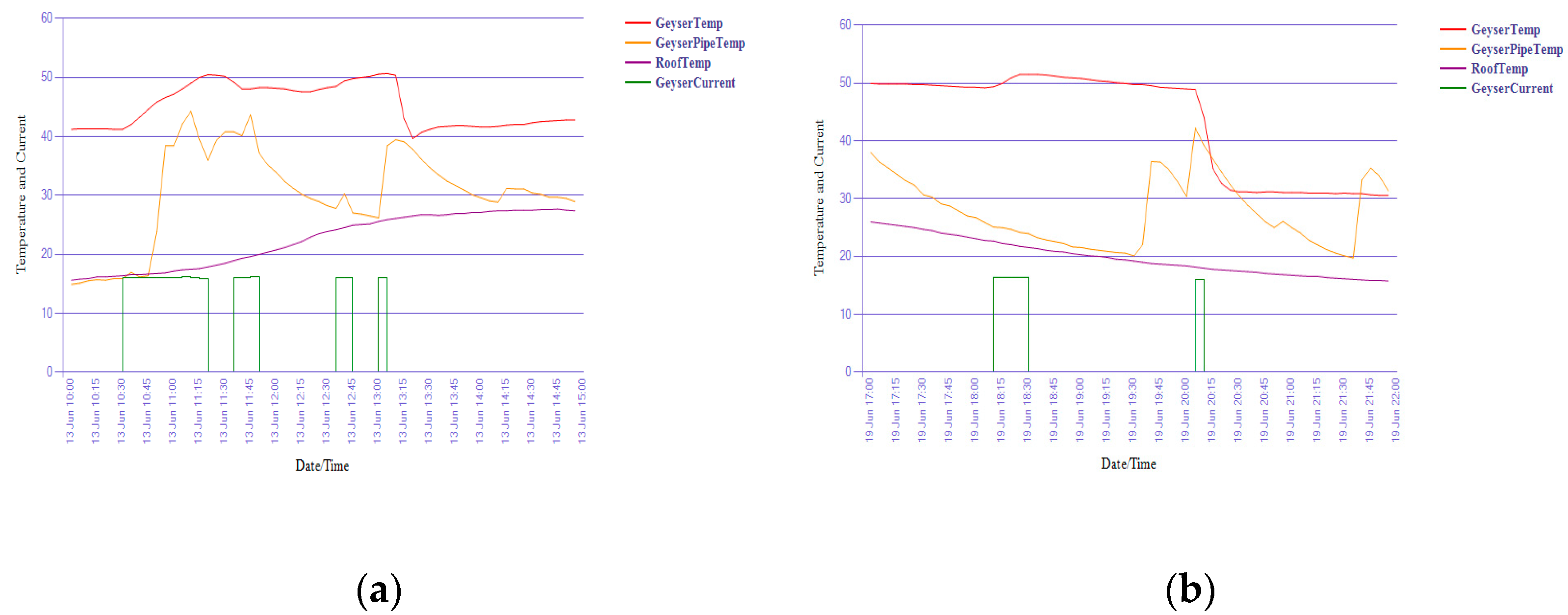
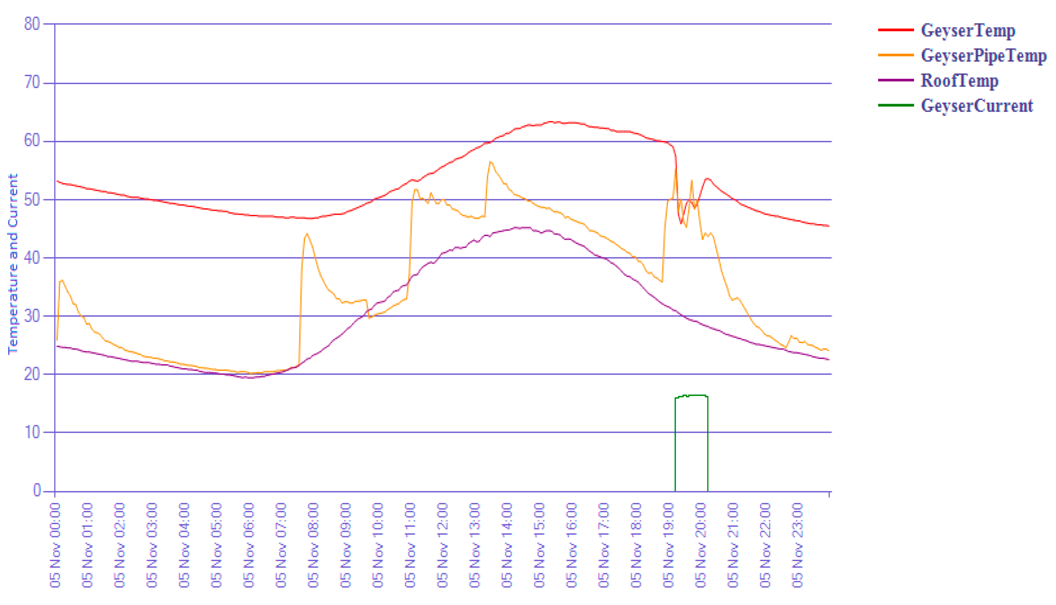
Geyser, pipe and roof temperatures with current recording are illustrated in Figure 5, depicting a clear difference between a shower and bath usage.
Specifically, Figure 5a illustrates that the geyser temperature dropped by 10 °C when a shower is taken against 20 °C in Figure 5b when a bath is taken during one of the winter months. The same effects are noted during the summer months but with an average 8 °C when a shower is taken compared to 15 °C when a bath is taken during the same period.
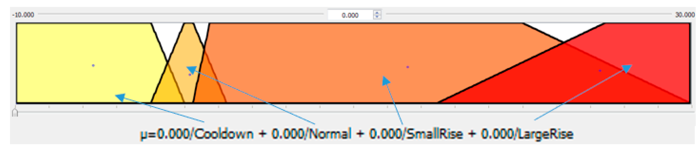
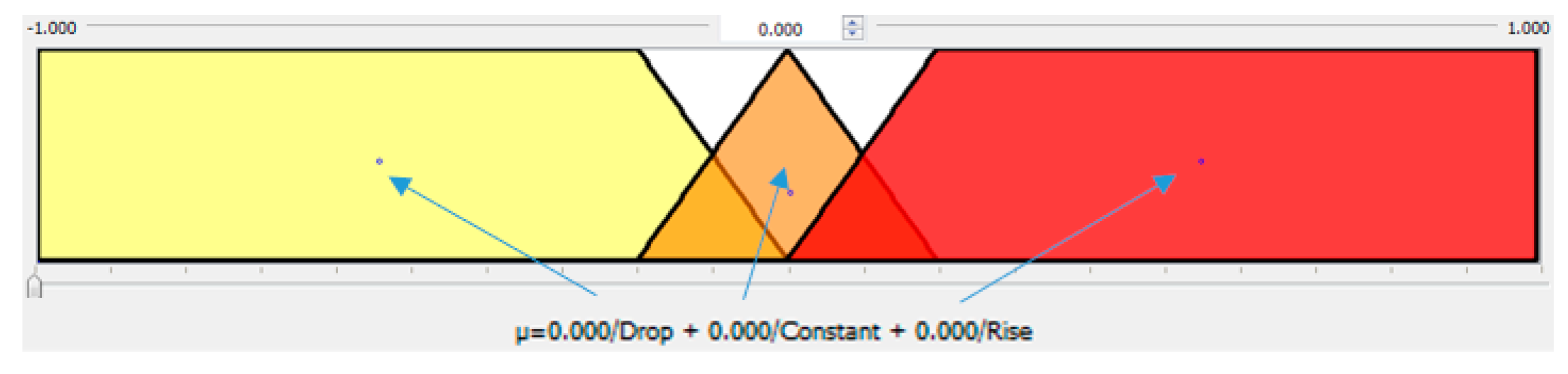
Fuzzy logic is used to group the geyser usage into fuzzy linguistic terms: None, Small, Medium and Large. Sensors are used to record a month of data included in the fuzzy set [17]. Fuzzylite 4.0 [18] is used in this research to develop fuzzy sets before it is implemented into the controller. The delta values for each membership function were taken over five-minute periods and the highest usage per hour is recorded for further predictions. The shape of a membership functions is defined mathematically by various shapes and is dependent on the purpose. Zadeh et al., classified the membership functions into two groups: Linear and Curved. A membership function µA(x) defines the degree in which x verifies in the fuzzy set [19], depicted in Equations (2)–(4). Roof temperatures are included in the fuzzy logic model to determine the difference between water pipe temperature increases and cool down effects from water usage or weather temperature changes. The roof temperature changes only influence None and Small usages. The three fuzzy sets created with multiple linguistic membership functions are illustrated in Figure 6, Figure 7 and Figure 8:
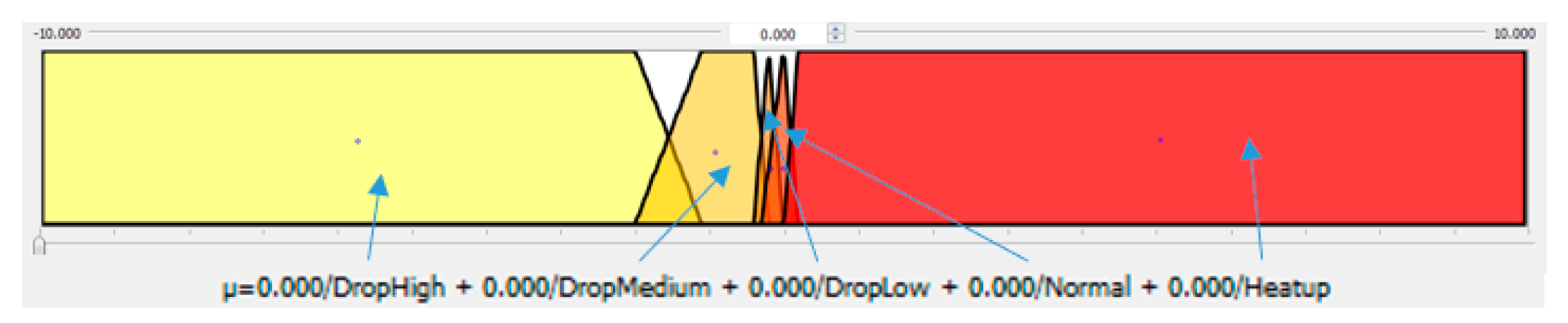
- DeltaGeyserTemp Set: DropHigh, DropMedium, DropLow and Heatup Membership;
- DeltaPipeTemp Set: CoolDown, Normal, SmallRise and LargeRise Membership;
- DeltaRoofTemp Set: Drop, Constant and Rise Membership function.
The pseudo code in Algorithm 1, illustrates the algorithm to “fuzzify”, inference and “defuzzify” the roof, geyser and pipe temperatures each five-minute interval to give a None, Low, Medium or Large output according to fuzzy logic controller design procedures. First fuzzification converts the physical input values into a normalized fuzzy subset and an associated membership function, which involves allocating suitable linguistic. The main purpose of this step is to make the input signal compatible with the fuzzy control rule base. The fuzzy set and the membership function need to be designed for each application and fuzzified warm water usages are as follows [20]:
µGeyserTemperature = (mx + c)/drophigh + (mx + c)/dropmeduim + (mx +
c)/droplow + (mx + c)/normal + (mx + c)/heatup
c)/droplow + (mx + c)/normal + (mx + c)/heatup
µPipeTemperature = (mx + c)/cooldown + (mx + c)/normal + (mx + c)/smallrise +
(mx + c)/largerise
(mx + c)/largerise
µRoofTemperature = (mx + c)/drop + (mx + c)/constant +(mx + c)/rise
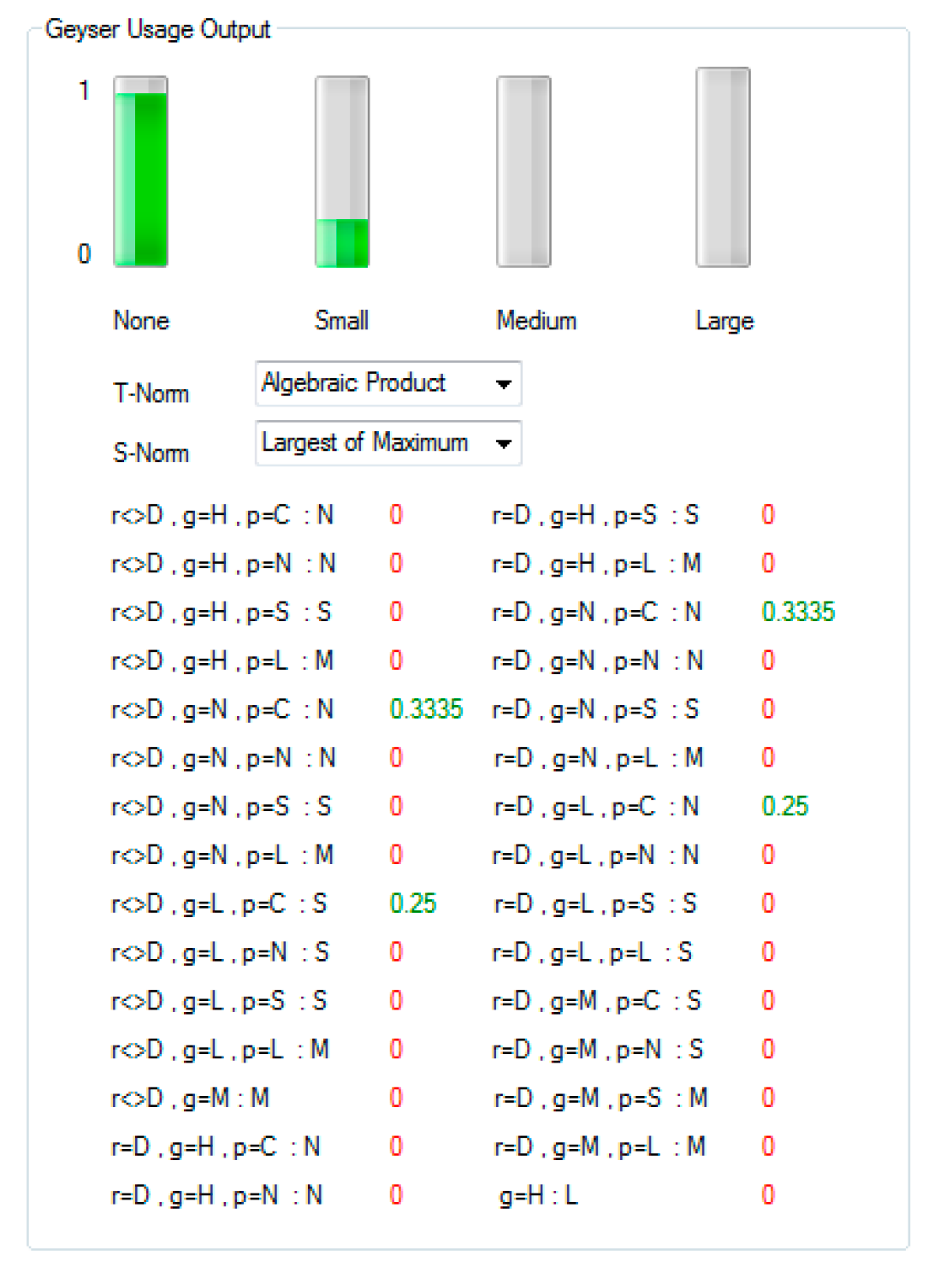
Next, the inference process, simulates human decision making based on linguistic rules to generate a fuzzy response [21]. The rule base depends on the developer expert knowledge about the specific system. The fuzzy logic controller needs to determine the choices in input and output variables for the IF THEN rules [17]. With simulations it was determined that the algebraic product for T-Norm used produced the best outcome during the inference phase with Equations (5) and (6) illustrating the calculations involved in rule 9 and 14, as shown in Table A1.
T-Norm9 = µDeltaRooTempNotDrop(1 − 0.5) × µDeltaGeserTempDropLow(0.5) ×
µDeltaPipeTempCooldown(1) = 0.25
µDeltaPipeTempCooldown(1) = 0.25
T-Norm14 = µDeltaRooTempDrop(0.5) × µDeltaGeserTempHeatup(0) ×
µDeltaPipeTempCooldown(1) = 0
µDeltaPipeTempCooldown(1) = 0
Appendix A displays the thirty rules created from the Fuzzy sets covering all the options satisfactory for this purpose. Lastly, defuzzification is the interface between the rule base and the application’s physical output control. It converts all the output membership function back to crisp terms using several common defuzzification formulas [17]. By means of a simulation-driven process it is determined that the largest of maximum as S-Norm produced the best outcome from all the sum off all inference calculated [21], as illustrated in Figure 9, where the best and largest crisp term is illustrated, and calculated as follows:
S-NormNone = 0.3335 + 0.3335 + 0.25 = 0.917
S-NormSmall = 0.25
S-NormMeduim = 0
S-NormLarge = 0
4.2. Profile Solar Geyser Heating
It is significant to predict the solar efficiency at the start of each day, to determine the optimal electrical energy that could be added to the water heating system. Partial partitioning is, therefore, used to create three medoids to simplify the investigation, by seeking for the relationship between environmental conditions and the solar heating efficiency [22]. This is needed, as the solar radiation predictions are not commonly available. Research done by Sauer et al., confirmed this as a suitable approach. By using clustering and HMMs, solar radiation can be calculated for a specific location [4]. To deal with large data sets, a sampling method called clustering large application (CLARA) can be used where only one random sample is taken to calculate the best medoids. This increases the processing time but decreases the possibility to select the best medoids drastically. An algorithm called clustering large Application, based upon randomised search (CLARANS), is used because it is a trade-off between cost and effectiveness. The algorithm selects n-times a temporally medoid and calculate if the newly selected medoid will improve the absolute-error criterion. If the error improves, the temporal medoid is chosen as the new medoid [23].
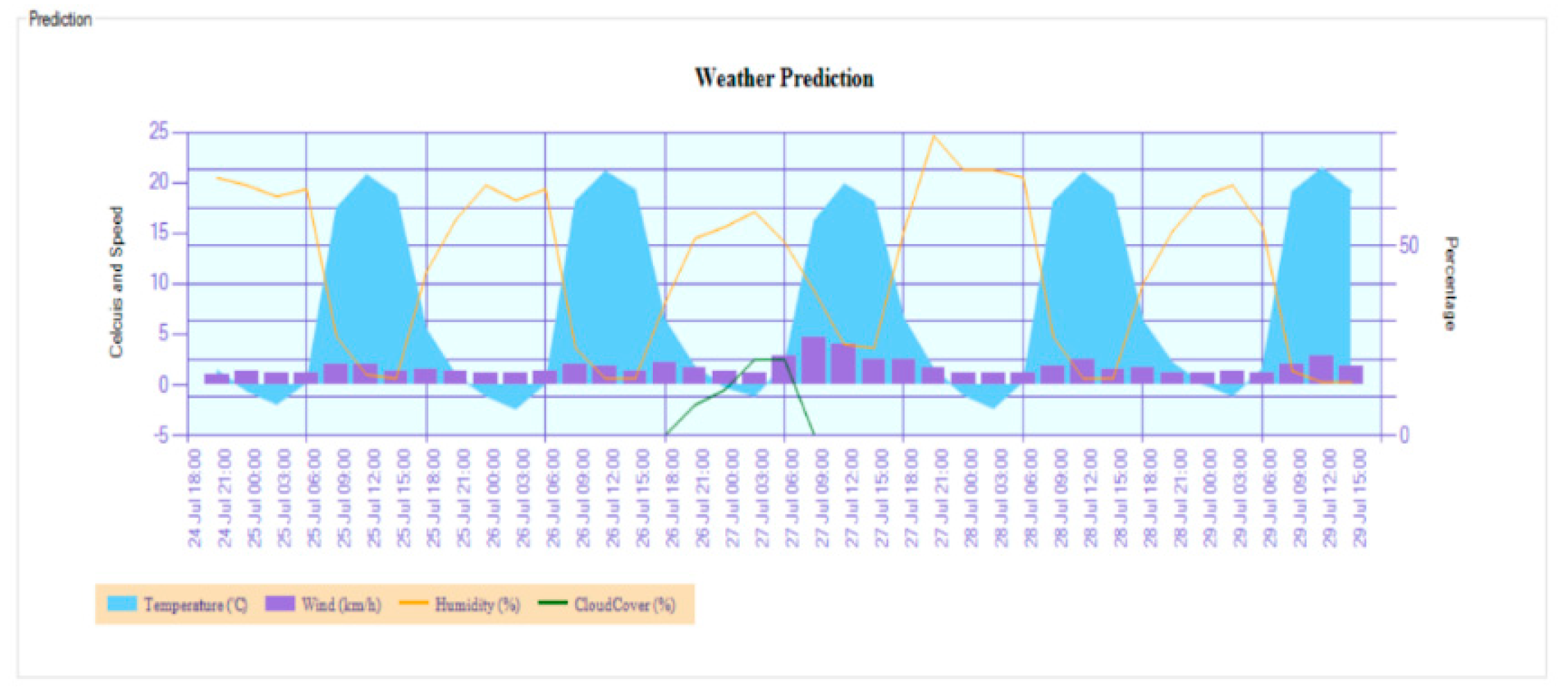
Instead of recording the weather conditions the official weather predictions are used as an internet-based sensor. Figure 10 illustrates the graphical interpretation of the xml file retrieved from openweathermap.org.
The influence of temperature, humidity, cloud cover and wind speed are investigated determining the factors required for the prediction algorithm. Maximum weather conditions between 08h00 and 14h00 are used as conditions outside these time periods had little to no influence on the solar heating as illustrated in Figure 11.
The historical geyser water temperature could not be used as a reference point, because it is a combination of electrical and solar energy added to the system. Electrical energy could have been added to the system if the water is too cold. Taking the water temperature would indicate a higher temperature as what is possible via solar energy for the day. The roof temperature is used to calculate the amount of solar energy added to the warm water (geyser temperature) as there is a close relationship between them illustrated in Figure 11.
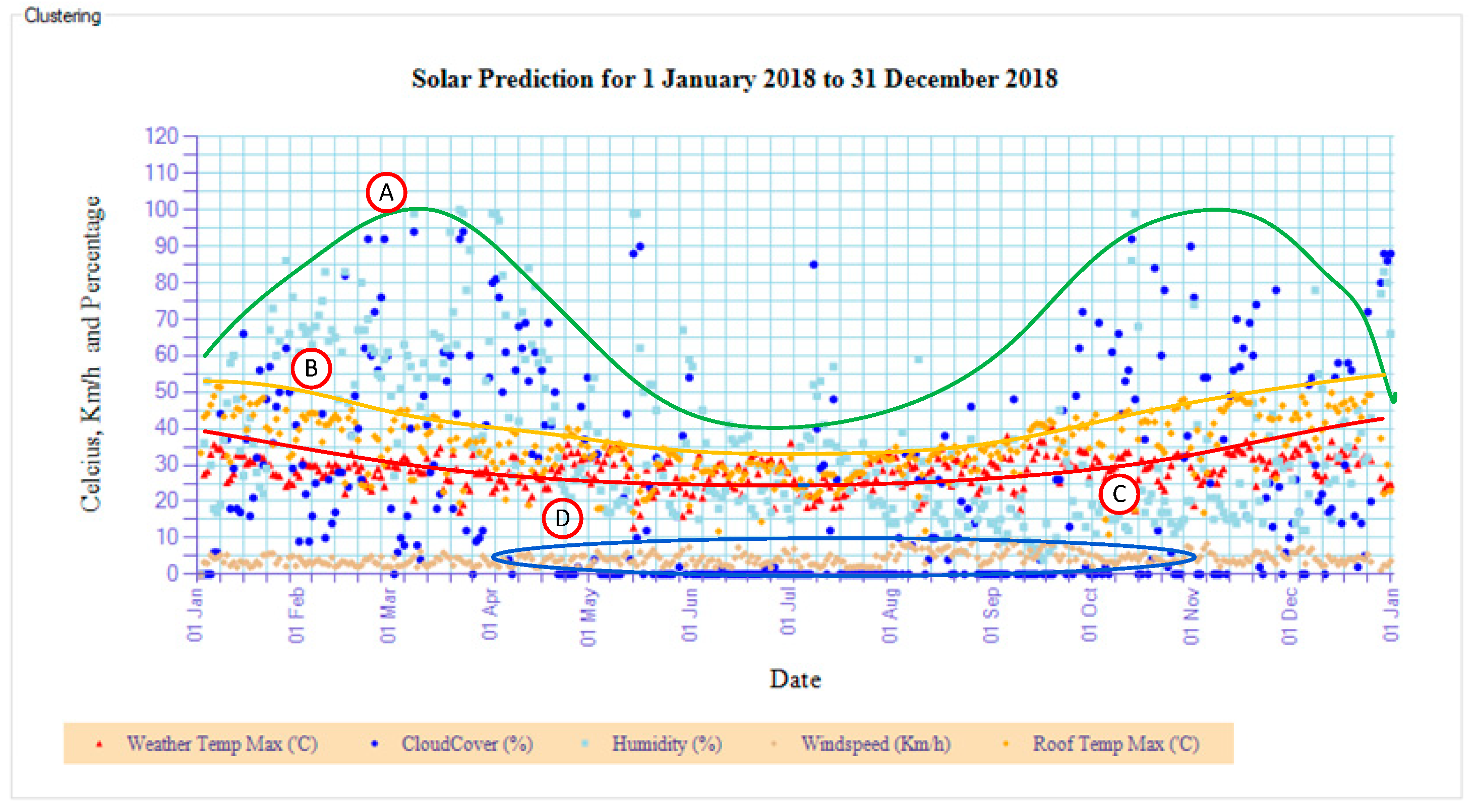
The daily maximum temperature, cloud cover, humidity wind speed and roof temperature for 2018 are shown in Figure 12. The green line, labelled A, illustrates the maximum daily cloud cover and humidity trends, the orange line, labelled B, the recorded maximum roof temperatures and the red line, labelled C, the maximum temperatures. Cloud cover and humidity do not have any significant influence during the colder winter month to the roof temperatures. Label D illustrated from middle April to end October that the cloud cover is 0%. Investigating the calculated medoids, three seasons are classified:
- Rainy season: High (January, February, March, April) where cloud cover and humidity goes above 70%;
- Rainy season: Low (October, November, December) where only cloud cover goes above 70%;
- Rainy season: None (May, June, July, August, September) where cloud cover and humidity readings are below 70% on average.
The hidden Markov model is used to predict the solar efficiency from the weather patterns, as HMM utilizes a double stochastic process with underlying stochastic process that is not observable. This hidden layer can only be observed through another set of stochastic processes that produce the sequence of observed symbols as required [24]. The probability of the output only depends on the current state in which the Markov vhain is in [25]. HMM defines the initial state probability, transition probability and observation or emission probability as:
where, P is the probability, N is the number of hidden states, V refers to the set of distinct observations observed, M is the number of distinct observations per state, St is the state at time t, qt is the current state at time t and vk is the kth observation symbol. λ represents the complete parameter set of the model where [26].
Initial state probability: πi = P[q1 = si], 1 < i < N
Transition probability: aij = P[qt = sj | qt−1 = Si], 1 < i j < N
Emission probabilities: bj(k) = P[vk at t | qt = Sj], 1 < j < N, 1 < k < M
λ = (A, B, π)
Three basic problems must be solved for HMM to be useful in real-world applications. (1) Evaluation. Given O and λ, how can the probability of a given model producing the output sequence P(O|λ) efficiently be computed? A solution is the forward algorithm; (2) Decoding. Given O and λ, how can a given sequence Q = q1, q2…qT best explains the observations O? A solution is the Viterbi algorithm; and (3) Learning. Given O, how to choose a model parameter λ to maximize P(O|λ)? A solution is the Baum–Welch algorithm. Where O is the observation sequence and Λ is the hidden Markov model [27]. In other studies, ambient conditions are used predicting weather patterns.
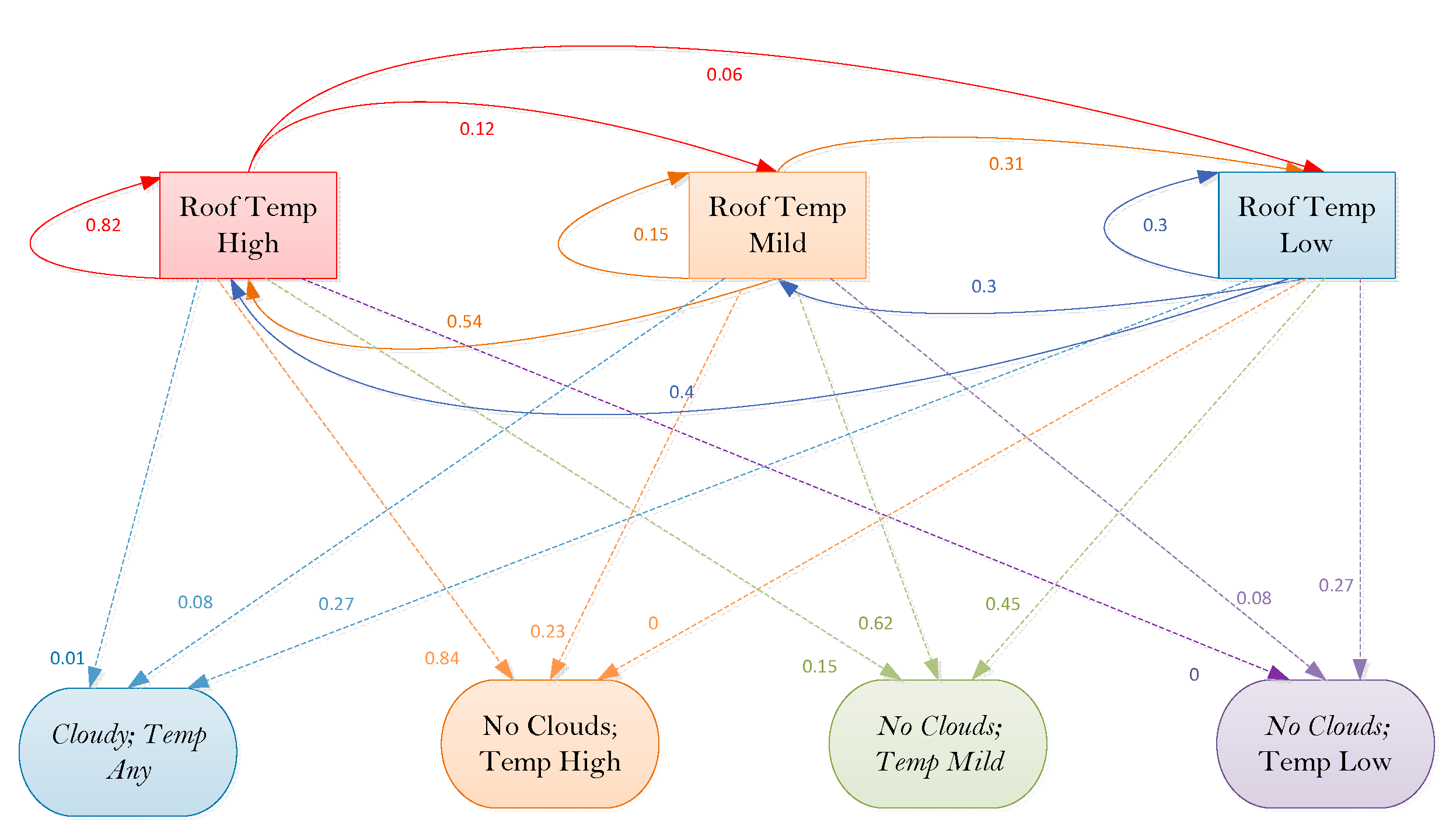
In this study, the weather predictions are used as the known observations and the water heating as the hidden component. First, three HMM modules are built, one per season which are: High, Low and None. The expected outcome from the HMM is the probability to maximize the heating process with solar radiation from weather predictions. In creating the HMM an assumption is made that the normalised values between 0 and 0.32 will be Low, 0.33 to 0.65 Medium and 0.66 to 1 High for temperatures and 0 to 0.69 Low and 0.8 to 1 High for humidity and cloud cover. An assumption is made based on historical data to classify cloud cover and humidity above 70% together as cloudy, preventing using multiple order HMM. Figure 13 illustrates the roof and weather HMM initial state, transition and observation probability distribution for the low rainy season.
5. Results and Discussion
This section covers the HMM training process to predict the geyser’s warm water usages and solar heating. These predictions are calculated when the electrical backup element must be enabled producing a balance between human convert and saving electrical energy.
5.1. Profile Solar Geyser Heating
Training the HMM, Baum–Welch algorithm was used with the forward/backwards algorithm. A set of reasonable re-estimation formulas for A, B, π are in [30].
π‘i = expected number of times Si at time (t = 1)
The first problem encountered, when one year’s data is simulated, is that the module starts getting stuck into a specific prediction. Investigating the HMM trained transition and emission values it is found that certain values become zero. Equations (15)–(17) are used to train the module. It is evident that the values used to multiplying or dividing, resulting in an outcome of zero or undefined. The outcome is that certain predictions are fixed as a 1 or 0, as shown as prediction b represented by Equation (18).
Resolving the stuck in local maxima appearance by first ensures that no HMM model values are 1 or 0 [31]. Another problem is that after the Baum–Welch algorithm alters the model values the sum of the normalised values are not always 1; this is referred to as the label bias problem. First the model values are re-normalised after every Baum–Welch calculation. Pseudo code in Algorithm 2 shows the solution adopted to ensure no HMM values are represented by a zero. By subtracting 0.01 from the highest prediction and adding it to the zero valued probability ensuring the lowest value can only be 0.01. The same process is followed for the other HMM Initial, Transition and emission values. These modifications are shown as modification 1:1 to modification 1:3 in pseudo code in Algorithm 3. It also illustrates a detailed flow chart after observation state Cloudy is calculated. The same flow chart can be used for other observation states, as WeatherCloudy by replacing it with WeatherHigh, WeaterMild and WeatherLow depending on the observation states. The forward algorithm [32] is used determining the re-estimated transition probability α as illustrated in example 1 in the Appendix B. Partial partitioning medoids did indicate that yearly historical data indicate a weather trend, but it could not be used to make next day prediction. If less historical data is used, sudden changes in weather prediction have a higher accuracy. This however, with the less historical data, lost the knowledge that the probability is higher for a warm day during the summer than winter months. Through altering this amount of data, the best Baum–Welch results are obtained by using a combination of old data and new to an 8:2 ratio illustrated as modification 2, as depicted in the pseudo code in Algorithm 3 and Mod1 in Figure 14.
Figure 14 illustrates the Baum–Welch border and correct trained prediction comparison between different observation length and with and without the 8:2 yearly and daily data used. An observation length of seven days with modification did result in highest correct and lowest incorrect prediction over 12-month period. Viterbi algorithm is used, predicting the next day’s solar efficiency from daily HMM trained by Baum–Welch algorithm.
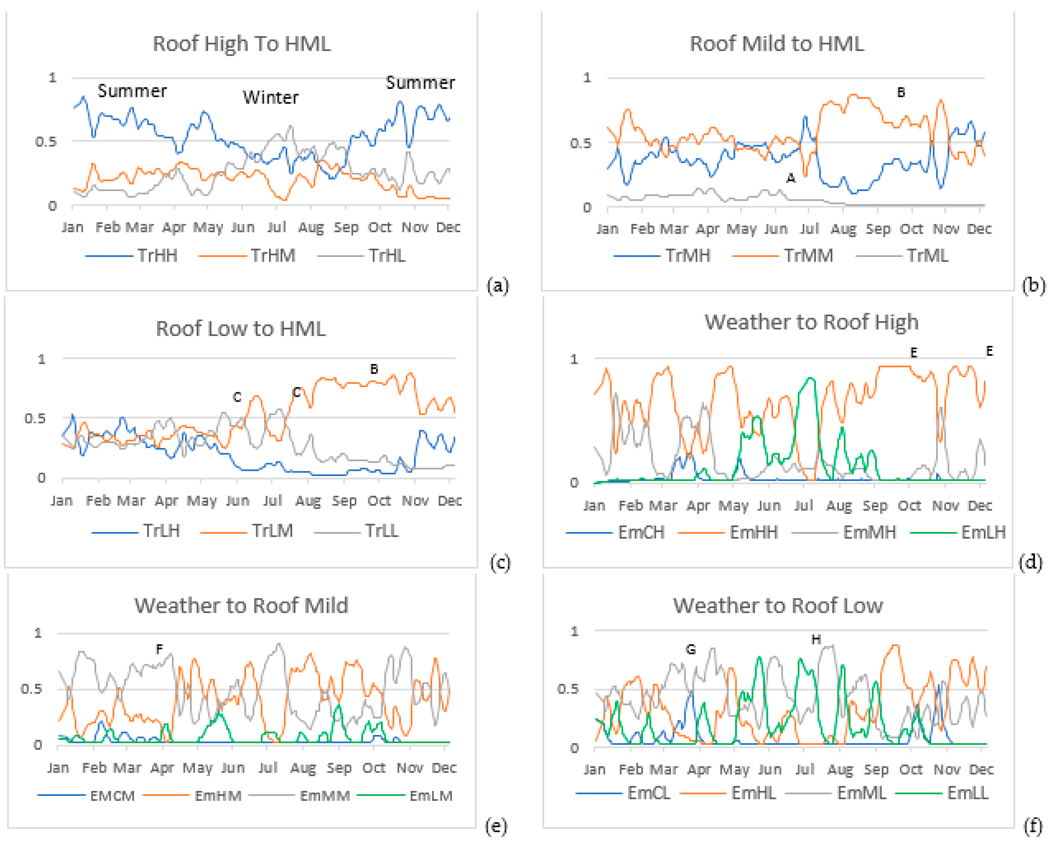
Figure 15a–c indicates the Baum–Welch output for the trained roof probalities from high to any, mild to any and low to any, where HML indicates the roof temperatures high, mild and low. TrHM for example in Figure 15a indicates the transition probabiliy for the roof temperature changing from a high temperature to a mild temperature. Figure 15a illustrates the probability for a high following by a high is the best during the summer and high following by a low during the winter. Point A, illustrates that the probabilities are low for the entire year for a mild temperature to be followed by a low temperature. Point B highlights that during spring and early summer the probability is the highest for a mild roof temperature. During winter, June and July at point C, there are periods where a Low temperature is the best followed by a Low at point D, but around start July the probability is better that a mild temperature will follow a Low temperature at point C. An explanation for that is when the last cold fronts for the winter season passed throught the area monitored. Figure 15d–f illustrates the emission probabilities between the weather conditions and the roof temperatures where for example EmCL indicates the probability that the roof temperature will be low when the weather condition is cloudy. The diagrams illustrate the HMM model train correctly between seasons and points E illustrates that the best scenarios for high are during spring and early summer months which are between September and December. During the rainy season, February to April, the probability where the best for a mild roof temperature as shown at point F, a mild followed by a low shown at point G and low temperature during winter shown at point H.
5.2. Warm Water Probabilities
As all the data is processed by means of a fuzzy logic approach, and with no hidden component, the probability that the water usage is None, Small, Medium or Large is calculated by the sum per usage, divided by the sum of samples as defined by Bayes’ theorem where [33]:
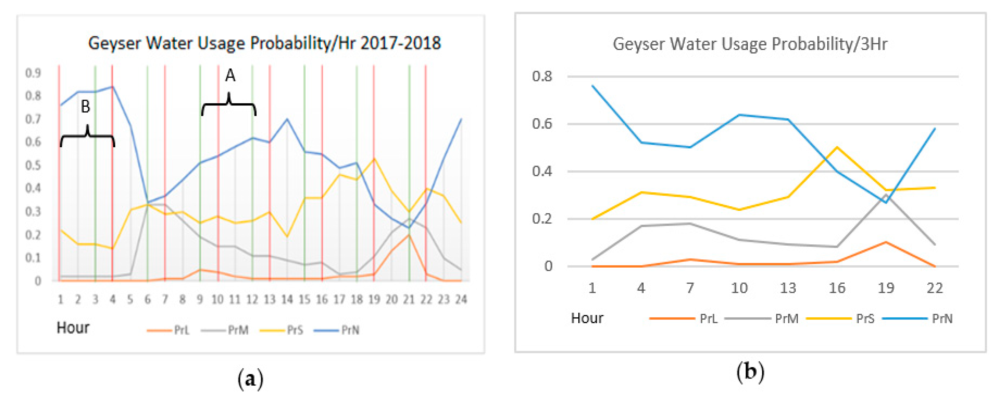
Keeping track of usage per hour is the most accurate approach, but this also requires the most processing and memory resources. To investigate Figure 16a further, the readings are divided into three-hour slots. First, timeslots are created starting from 0h00 to 2h59, 3h00 to 5h59, …., until 21h00 to 23h59, as indicated with the green lines marked as A. The warm water usage only changes from None too Small between 4h00 and 5h00. The system must start heating the water before 3h00 to ensure correct water temperature starting timeslot 3h00 to 05h59. If the timeslots are forwarded with an hour, as illustrated by the red lines and marked as B, the timeslots will be from 1h00 to 3h59, 4h00 to 6h59, …., until 22h00 to 0h59 presentation the warm water usage better. The Large usages also fall in the timeslot 19h00 to 21h59, otherwise the system would require heating the water for Large usage also between 21h00 and 23h00.
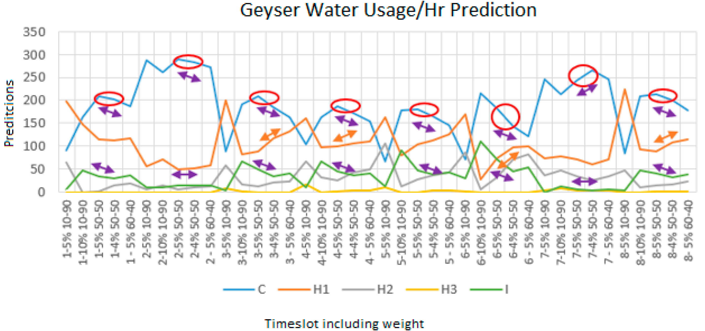
Figure 16b illustrates the warm water usage per three-hour timeslots. It is notable that the trend of usage per hour and three hours did stay the same with a low level of loss in weight per category per timeslot. The same principle is used training the water usage probability per three-hour slots, as heating the water with solar energy by using a combination of historical and Baum–Welch calculated values. Figure 17 illustrates the influence on prediction through two factors. First, the percentage historical with new seven days calculated prediction. The x-axis category “1 5% 10–90” means the following: Timeslot 1, highest weight usage 5%, 10% seven day and 90% historical data used. The label represents the water usage predations where C represents the water usage predicted correctly, H1—the geyser water is heated one usage class higher, H2—two water usage classes higher, H3—three water usage classes higher and I—indicates that the water is heated to cold. An example of one water usage class higher is when the water was heated for large usage, but only medium water usage was used. The one to eight (x-axis) indicates the eight timeslots.
Figure 17 also illustrates the results between 10–90%, 50–50% and 60–40% weight that the highest number correct predictions were the sum of 50% historical and 50% previous seven days prediction as indicate with the red highlights. With 50–50% given the highest correct predictions changing the highest used weight from 5% to 4% the number correct predictions decrease but also the number of incorrect predictions as indicated by the purple arrows. A steep increase in H1 (Water heated on class higher then needed), orange arrows is noted. A small inline is also noted at H2. Lastly, a higher value of the condition “highest used weight” will produce better power savings but lower human satisfaction, where lower value of this condition “highest used weight” will produce lower power savings with higher human satisfaction. By means of simulation it is determined that the highest percentage usage per timeslot cannot be obtained by using data of the 14 January 2018 Timeslot six for example: None 45%, Small 42%, Medium 8% and Large 4%. The system could not produce a result of usage that is represented by None. A new variable is included determine from UsageHigh to UsageLow the minimum percentage used, determining the usage selection. For example, if the cut-off is 5%, the prediction will be Medium but if the cut-off is 4% the prediction will be Large.
5.3. Combining Water Usage and Solar Heating Predictions for Controlling Geyser Element
To conclude the combining of the solar geyser heating prediction and warm water usage prediction together, to determine when and by which factor, an electrical energy must be injected to the geyser with an electrical standby element if solar energy will not be sufficient to supply hot water for a specific period. The system did require the cooling period and some geyser parameters are challenging to collect due to the thickness of insulation, thermal conductivity and surface heat transfer coefficient. A function is therefore added to calculate the loss parameter Δx /k + 1/h in Cm2/J according to Equation (1) from historical recordings. Investigating the recordings, a suitable condition is found to be between 24 March 2018 00h30 to 03h30, where the ambient temperature dropped from 17.2 °C to 17.1 °C. All the other parameters are predefined and by calculating the loss parameter as 3.638 × 10⁻⁴, resulting in 222.9333 kJ losses per hour. The heating period is calculated by how much energy needs to be added to the system with Q = mcΔT where m is the mass in litres of water, c = 4180 Joules per litre per °C [14,34] and ΔT is the change in temperature in °C. The system requires some user input, as there required temperature for timeslot with prediction None, Small, Medium and High usage for a cold day, which is lower than 25 °C and a warm day. Pseudo code in Algorithms 4 and 5, illustrates the prediction, if the element must be switched on or off. The algorithm requires knowledge of when the next timeslot started. Time-based controllers start heating the water at a specific time of day. This algorithm already has the knowledge of the geyser parameter and calculates the start time to heat the water, having the correct water temperature entering a specific timeslot. The following rules are implemented in the prediction model:
- Except for timeslot four to six, no solar heating will be included to determine if geyser element must be enabled.
- For each timeslot, the current and next timeslot minimum temperatures values were retrieved.
- Every five minutes or when temperatures changes, the time-period not elapsed in timeslot and time required to heat water from current temperature to next time slot are calculated.
If the geyser water temperature is lower than the required temperature and the water is not busy with cooling down period, the element is switched on. The cool down period is enabled when required water temperature is reached and disabled when water is cooled down for 5 °C eliminating geyser switch on/off the entire time if temperature drops 0.1 °C and switch of seconds later when required temperature is reached (to implement hysteresis). The geyser will also be switch on, if the water temperature is correct for required timeslot, but the time left at current timeslot is less or equal than the time needed to heat the water to minimum temperature for next timeslot. During timeslot four, the next timeslot which starts at 10h00, the process changes heating water for the next timeslot. As it is still early in the morning the element will heat up the water except if the solar prediction is High. During the middle of the day, which is timeslot five and six, the element will only be enabled for current and next timeslot temperatures if the solar prediction is Low.
For the most accurate data, the simulations were done continuously from 11 January 2018 until 21 December 2018, and not per day. Figure 18 and Figure 19 illustrates two samples taken.
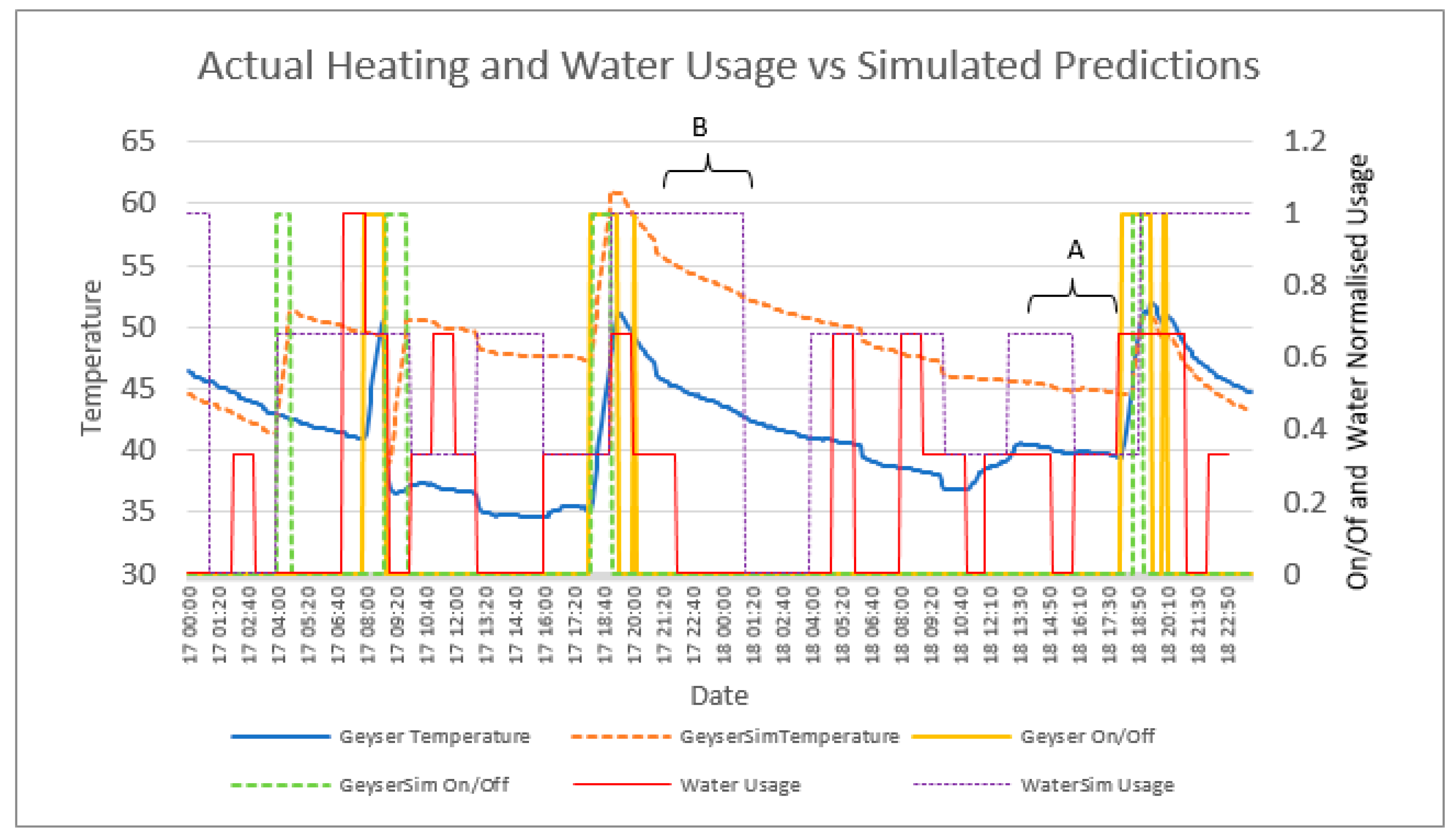
The difference between controlling the geyser element with a time-based controller against a controller with solar heating and warm water usage that can adopt to external changing factors are shown in Figure 18 with the same warm water usage. The figure illustrates the comparison over a weekend starting Saturday with cloud cover up to 90% during the solar heating time periods. Investigating the effects over two days illustrates a more accurate representation if solar heating is inefficient. Investigating the 17 March 2018, it is shown that the algorithm predicts a medium use on a cool day. At 08h00 there is a large usage and no heating was required before the time. Compare this with the recording it is notice the water was heated and used just afterwards, indicating that the controller was override as there was no warm water to use. Afterwards, the water was not heated leaving the household with cold water the entire day. The simulator did have knowledge of the weather prediction and heated the water with the element. Both controller and simulator incorrectly heated the water the afternoon for a large usage, as it was already implemented earlier the day.
The Sunday, at point A, it is noticeable that the recordings shown between 10h00 and 13h00 an increase in temperature and indicate it is done through the solar collector, as the element is not activated. As the simulation heat the water at point B and no Large warm water usage occur, resulting that the water is warmer, as which the solar collector could heat the water at point A. This indicate in an incorrect prediction to heat the geyser water at point B, but it did result in warmer water the entire 18 March. Starting at the 17th, the recordings indicate the water is 2 °C higher than the simulation and at the midnight, the 18th, the recorded temperature is 1 °C higher than the simulator with the simulator activated the element for 3 h against the recorded 3.91 h.
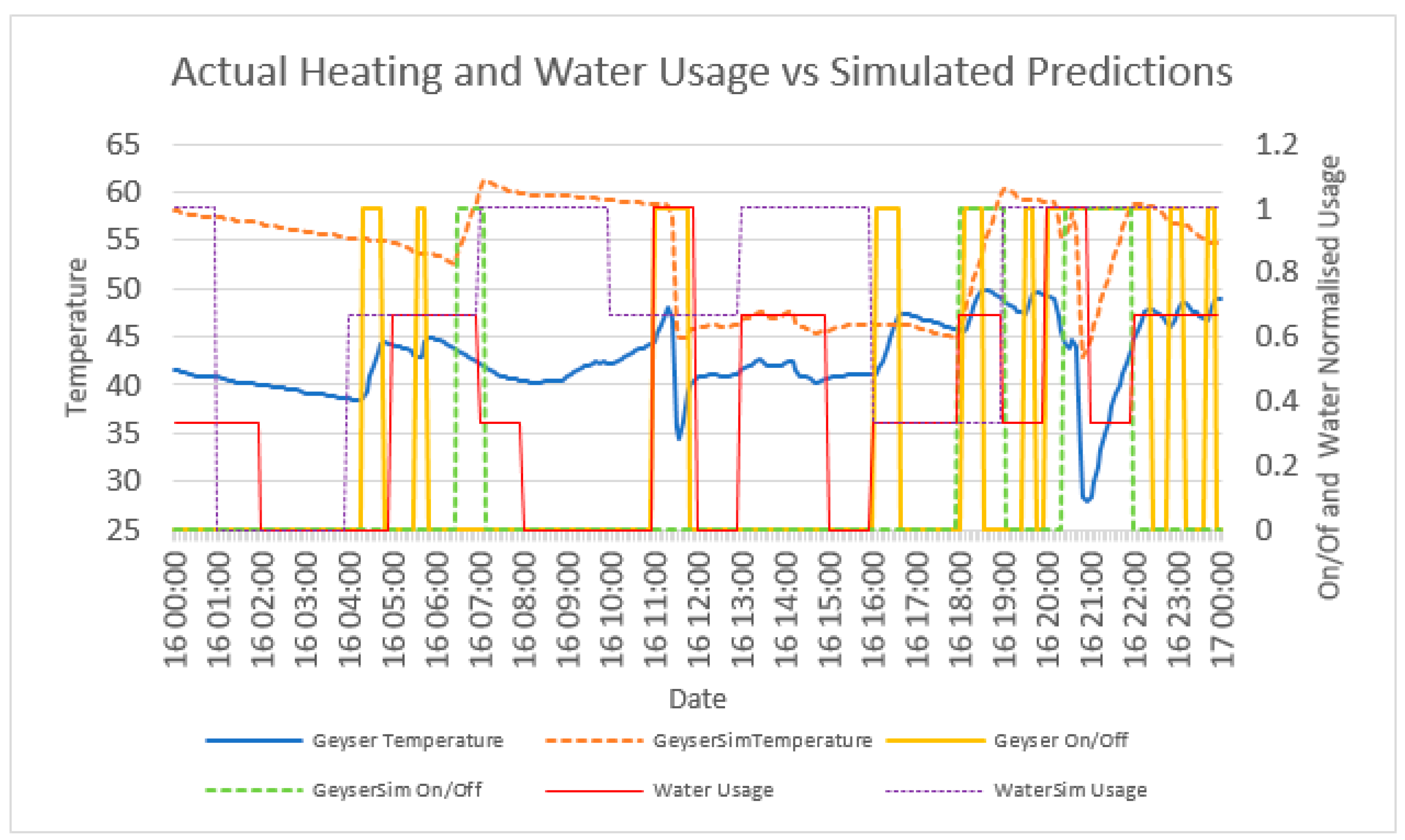
Figure 19 investigates 16 July 2018, illustrates the comparison between the simulator and recording for a cold clear winter’s day. There are two large usages at 11h20 and again at 20h40. It is noted that the simulator did heat the water, with higher temperatures as the recordings with the element activated for 2 h and 10 min against the recorded 5 h and 55 min.
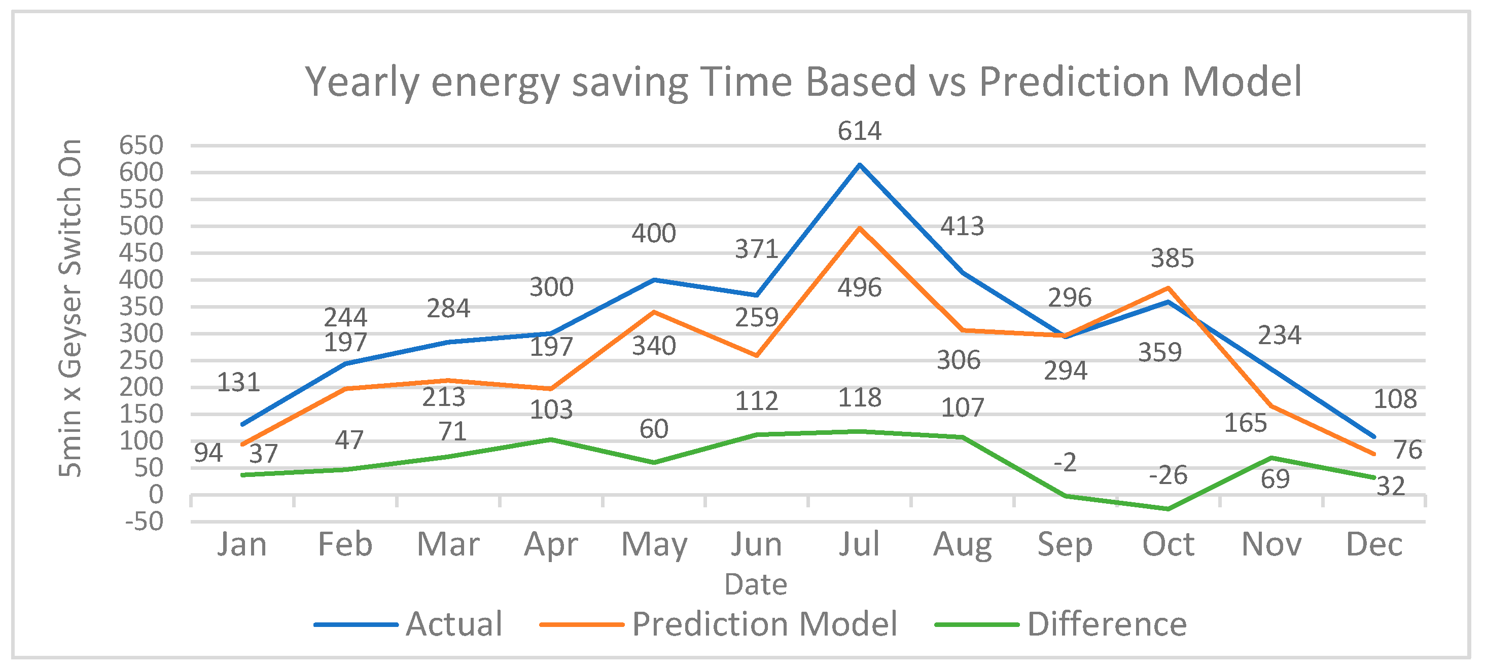
Appendix D illustrates a sample of the calculations of the geyser water usage to the geyser water prediction training. Figure 20 shows a yearly comparison between the algorithm simulation and the recordings. As expected, both did activate the element more during the winter with July, the most and the dry summer month December and January the least.
The algorithm did activate the element less for all months as can see for example during Jun the prediction module activated the element 259 timeslots against the actual 371 timeslots, except for September and October where the simulation did activate the element 2 and 26 timeslots more than that was recorded with a time-based controller. The simulator is activated 728 times 5 min less, result in 61 h per year. As most off the savings in heating water are already accomplished by installing a solar collector and a warm water time-based controller. There is no major saving in the electrical bill, but it is proved that a controller that has knowledge of external conditions switched the element 3024 five-minute intervals against 3752 five-minute intervals. In the simulation the intelligent controller switched the element 728 times less and is 19.4% more efficient than a time-based controller with higher warm water temperatures during the day. The biggest advantage is a higher customer satisfaction as there are fewer occasions that the controller must manually activated or re-programmed.
6. Conclusions
The study was applied on a time-based controlled solar heated geyser environment. Human behaviour was incorporated as a criterion as sensor readings change with the withdrawal of hot water from the system. Thus, addressing event classification correctly, for the model to be able to differentiate between sensor reading fluctuations by an event or environmental conditions. For example, the drop-in temperature during night-time had the same behaviour on the pipe temperature as the use of a small amount of hot water. Membership functions were correctly created to categorise changes in water pipe temperatures as water usage or increase or decrease in ambient temperatures.
Partial partitioning were implemented to analyse the data, creating medoids, simplifying and analysing thousands of recorded entries. This produced a result of a certain pattern associated per season. Implementing yearly or monthly historical data did not indicate accurate prediction probabilities for the newly develop prediction model. Analysing the data, clarified that a combination of all historical data (yearly, monthly, weekly and daily) must be used with a different weight, to increase the prediction model accuracy.
By implementing the standard Baum–Welch algorithm to resolve hidden Markov model’s training, it was found that if the observation sequence was too long, the probabilities could become zero, resulting in local maxima appearance. This scenario was a different outcome to that which was expected based on the related literature, as when the hidden Markov model is employed in other applications the predictions become more accurate with larger observation sequences (for example within robotics or speech recognition applications). The standard hidden Markov model with Baum–Welch was found not to be suitable to train the model for sudden environmental and human behavioural changes. If the standard hidden Markov model was used, multiple HMM models were required, as each season observation was different and did decrease the accuracy of one global model. Another shortcoming encountered with the standard Baum–Welch backwards algorithm was that it did not include the current training forward (α) calculations. This was another factor that made the standard HMM slow in adopting in sudden environmental or human behavioural changes.
Combining historic and seven-day historical recordings (with a weight of 90% for all historic recordings and 10% for the past seven days), made the model sensitive to sudden changes in weather conditions without the need to develop a new training model. The modified Baum–Welch algorithm resulted in the use of only one HMM model with no season specific knowledge with only five incorrect hidden Markov predictions for the year 2019.
Simulations on the overall system did indicate that the geyser controller was up to 20% more efficient than a time-based controller. However, though savings seemed minimal the most significant advantage was that more reliable hot water was provided when needed. New contributions made in this study by implementing the developed prediction model are as follows:
- Converting sensor readings into linguistic terms simplified the prediction.
- Altering the Baum–Welch algorithm by means of the hidden Markov model training by decreasing the length of the observations. Thus making the predictions more accurate through adding different weights to different age emissions and observation data for prediction models where sudden behavioural changes can occur.
- Proving that an artificial algorithm can be implemented in a smart home or office environment with the same comfort levels, but also reducing the electrical power usage.
The same algorithm can be applied to other large power consumption product like a swimming pool with solar panels. Future research can be done investigating additional saving by having different HMM’s for workdays, weekends and public holidays.
Author Contributions
Conceptualization, D.N.d.B. and B.K.; methodology, D.N.d.B. and B.K.; software, D.N.d.B. and B.K.; validation, D.N.d.B. and B.K.; formal analysis, D.N.d.B. and B.K.; investigation, D.N.d.B. and B.K.; resources, D.N.d.B. and B.K.; data curation, D.N.d.B., B.K. and W.H.; writing—review and editing, D.N.d.B., B.K. and W.H.; visualization, D.N.d.B. and B.K.; supervision, B.K.; project administration, D.N.d.B. All authors have read and agreed to the published version of the manuscript.
Funding
This research received no external funding.
Institutional Review Board Statement
Not Applicable.
Informed Consent Statement
Not Applicable.
Data Availability Statement
The data presented in this study are available on request from the corresponding author.
Conflicts of Interest
The authors declare no conflict of interest.
Appendix A

Table A1.
Fuzzy rules fuzzified Roof, Geyser and Roof temperatures.
| Rule | DeltaRoof | And DeltaGeyser | And DeltaPipe | Usage |
|---|---|---|---|---|
| 1 | not Drop | Heatup | Cooldown | UseNone |
| 2 | not Drop | Heatup | Normal | UseNone |
| 3 | not Drop | Heatup | SmallRise | UseSmall |
| 4 | not Drop | Heatup | LargeRise | UseMedium |
| 5 | not Drop | Normal | Cooldown | UseNone |
| 6 | not Drop | Normal | Normal | UseNone |
| 7 | not Drop | Normal | SmallRise | UseSmall |
| 8 | not Drop | Normal | LargeRise | UseMedium |
| 9 | not Drop | DropLow | Cooldown | UseSmall |
| 10 | not Drop | DropLow | Normal | UseSmall |
| 11 | not Drop | DropLow | SmallRise | UseSmall |
| 12 | not Drop | DropLow | LargeRise | UseMedium |
| 13 | not Drop | DropMedium | UseMedium | |
| 14 | not Drop | Heatup | Cooldown | UseNone |
| 15 | not Drop | Heatup | Normal | UseNone |
| 16 | not Drop | Heatup | SmallRise | UseSmall |
| 17 | not Drop | Heatup | LargeRise | UseMedium |
| 18 | Drop | Normal | Cooldown | UseNone |
| 19 | Drop | Normal | Normal | UseNone |
| 20 | Drop | Normal | SmallRise | UseSmall |
| 21 | Drop | Normal | LargeRise | UseMedium |
| 22 | Drop | DropLow | Cooldown | UseNone |
| 23 | Drop | DropLow | Normal | UseNone |
| 24 | Drop | DropLow | SmallRise | UseSmall |
| 25 | Drop | DropLow | LargeRise | UseSmall |
| 26 | Drop | DropMedium | Cooldown | UseSmall |
| 27 | Drop | DropMedium | Normal | UseSmall |
| 28 | Drop | DropMedium | SmallRise | UseMedium |
| 29 | Drop | DropMedium | LargeRise | UseMedium |
| 30 | DropHigh | UseLarge |
Appendix B
Example 1: Forward algorithm determine α
h = Hot, m= Medium, l = Low
O = H,H,H,H,H,H,H,H
Π =
A =
B =
The first Equation (18) is modified, as illustrated in pseudo code in algorithm 3, modification 1-x, not consists of any zero’s or one’s.
B =
The initial forward parameters calculated is based on the first weather observation and the mathematical formula for the complete process is
αt(i) = π i biO1 where 1 < i < N
The forward values at T = 1 are calculated as follows:
Ot = H where t =1
α1(h) = πh × bhh = 0.48 × 0.94 = 0.4512
α1(m) = πm × bhm = 0.34 × 0.7 = 0.238
α1(l) = πl × bhl = 0.18 × 0.11 = 0.0198
The next stage is calculating the induction for the following observation sequences as
αt + 1(j) = [ Σ αt(i) aij ] bj Ot + 1
The forward values at T = 2 to T = 8 are calculated as follows:
Ot = H where t = 2
α2(h) = [(α1(h) × ahh) + (α1(m) × amh) + (α1(l) × amh)] × bhh
= [(0.4512 × 0.75) + (0.238 × 0.19) + (0.0198 × 0.22)] × 0.94 = 0.36469744
α2(m) = [(α1(h) × ahm) + (α1(m) × amm) + (α1(l) × aml)] × bhm
= [(0. 4512 × 0.17) + (0. 238 × 0.62) + (0.0198 × 0.33)] × 0.7 = 0.1615586
α2(l) = [(α1(h) × ahl) + (α1(m) × aml) + (α1(l) × aml)] × bhl
= [(0. 4512 × 0.08) + (0. 238 × 0.19) + (0.0198 × 0.45)] × 0.11 = 0.0101486
The same process is followed for O3 to O8
α =
The final likelihood is calculated as
P(O|λ) = Σ αT(i)
The likelihood for the observation sequence is 0.132657661
Appendix C
The backwards algorithm [35] is used determining the re-estimated emission probability β. It requires the initial, transition and emission probabilities and the observation sequence and is explained in Example 2.
Example 2: Backwards algorithm determine β
The initial backward parameters calculated is based on the first weather observation and the mathematical formula for the complete process is
βT(i) = 1 where 1 < i < N.
The forward values at T = 9 is calculated as follows:
Ot = H where t = 8
β8(h) = 1
β8(m) = 1
β8(l) = 1
The next step is calculating the induction for the following observation where
βt(i) = Σ βt + 1(j) aij bj Ot + 1 where 1 < j < N and 1 < t < T − 1
The backwards values at T = 7 to T = 2 are calculated as follows:
Ot = H where t = 7
β7(h) = [(ahh × bhh × β8(h)) + (ahm × bhm × β8(m) + (ahl × bhl × β8(l)]
= [0.75 × 0.94 × 1] + [0.17 × 0.7 × 1] + [0.08 × 0.11 × 1] = 0.8328
β7(m) = [(amh × bhh × β8(h)) + (amm × bhm × β8(m) + (aml × bhl × β8(l)]
= [0.19 × 0.94 × 1] + [0.62 × 0.7 × 1] + [0.19 × 0.11 × 1] = 0.6335
β7(l) = [(alh × bhh × β8(h)) + (alm × bhm × β8(m) + (all × bhl × β8(l)]
= [0.22 × 0.94 × 1] + [0.33 × 0.7 × 1] + [0.45 × 0.11 × 1] = 0.4873
Ot = H where t = 6
β6(h) = [(ahh × bhh × β7(h)) + (ahm × bhm × β7(m) + (ahl × bhl × β7(l)]
= [0.75 × 0.94 × 0.8328] + [0.17 × 0.7 × 0.6335] + [0.08 × 0.11 × 0.4873] = 0.705393
β6(m) = [(amh × bhh × β7(h)) + (amm × bhm × β7(m) + (aml × bhl × β7(l)]
= [0.19 × 0.94 × 0.8328] + [0.62 × 0.7 × 0.6335] + [0.19 × 0.11 × 0.4873] = 0.433862
β6(l) = [(alh × bhh × β7(h)) + (alm × bhm × β7(m) + (all × bhl × β7(l)]
= [0.22 × 0.94 × 0.8328] + [0.33 × 0.7 × 0.6335] + [0.45 × 0.11 × 0.4873] = 0.342683
The same process is followed for O5 to O1
β =
The final likelihood is calculated as follows and must be the same as the forward likelihood calculated in Equation (13) [23].
P(O|λ) = [(πh × β1(h) × bhh) + (πh × β1(h) × bhh) + (πh × β1(h) × bhh)]
= [(0.48 × 0.2200 × 0.94) + (0.34 × 0.1212 × 0.7) + (0.18 × 0.101 × 0.96)]
= 0.1326576612
Appendix D
Sample of Geyser Usage Training Calculations

References
- Rea, M.S.; Figueiro, M.G.; Bierman, A.; Bullough, J.D. Circadian light. J. Circadian Rhythm 2010, 8, 17. [Google Scholar] [CrossRef] [PubMed] [Green Version]
- Bea, S.; Fang, M.Z.; Rustgi, V.; Zarbl, H.; Androulakis, I.P. At the interface of lifestyle, behaviour, and Circadian Rhythms: Metabolic Implications. Front. Nutr. 2019, 6, 2. [Google Scholar]
- Dintchev, O.D. Solar Water Heating as a Mechanism to Reduce Domestic Electrical Energy Consumption and Its Contribution towards South African Maximum Demand. In Proceedings of the 15th Domestic Use of Electrical Energy Conference, Cape Town, South Africa, 30 March–1 April 2006. [Google Scholar]
- Sauer, F.J. Predicting Solar Radiation Based on Available Weather Indications. Master’s Thesis, Missouri University of Science and Technology, Rolla, MO, USA, 2013. [Google Scholar]
- Delport, J. The Influence of Temperature on Residential Hot Water Load Control. In Proceedings of the 15th Domestic Use of Electrical Energy Conference, Cape Town, South Africa, 30 March–1 April 2006; pp. 2–3. [Google Scholar]
- LaMeres, B.J.; Nehvir, M.H.; Gerez, V. Controlling the average residential electric water heater power demand using fuzzy logic. Electr. Power Syst. Res. 1999, 52, 267–271. [Google Scholar] [CrossRef]
- Catherin, Q.S. Effective Geyser Management through Intelligent Hot Water Usage Profiling. Master’s Degree, Cape Peninsula University of Technology, Cape Town, South Africa, December 2009; pp. 51–56. [Google Scholar]
- Bakker, V.; Molderink, A.; Hurink, J. Domestic heat demand prediction using neural networks. In Proceedings of the 9th International Conference of System Engineering, Auckland, New Zealand, 1–3 September 2008; pp. 189–194. [Google Scholar]
- Hohne, P.A.; Kusakane, K.; Numbi, B.P. A review of water heating technologies: An application to the African context. Energy Rep. 2019, 5, 3. [Google Scholar] [CrossRef]
- Thomas, R.S.M.; Xia, X.; Zhang, J.F. Energy Efficient Geyser. In Proceedings of the 17th Domestic Use of Electrical Energy Conference, Cape Town, South Africa; 2008; pp. 3–6. [Google Scholar]
- Wolter, N.; Carrim, M.; Cohen, C.; Tempia, S.; Walaza, S.; Cohen, C.; Sibongile, W.; Sahr, P.; Gouveia, L.; Treurnicht, F.; et al. Legionnaires’ disease in South Africa 2012–2014. Emerg. Infect. Dis. 2016, 22, 131–133. [Google Scholar] [CrossRef] [PubMed] [Green Version]
- World Health Organisation. Legionella and the Prevention of Legionellosis; WHO: Geneva, Switzerland, 2007; p. 30. [Google Scholar]
- Geyserwise. Available online: http://geyserwise.com (accessed on 24 March 2019).
- Delport, J. The geyser gadgets that work/do not work. In Proceedings of the 14th Domestic Use of Electrical Energy Conference, Cape Town, South Africa, 29 March–2 April 2005; p. 3. [Google Scholar]
- Tooley, M.; Tooley, R. Exploring the Arduino Part 12: Wi-Fi and the Internet of Things. In Everyday Practical Electronics; Wimborne Publishing: Wimborne, UK, 2017; p. 41. [Google Scholar]
- ESP Basic. Available online: www.esp8266basic.com (accessed on 3 June 2018).
- Chen, G.; Pham, T.T. Introduction to Fuzzy Sets. In Fuzzy Logic and Fuzzy Control Systems; CRC Press: Houston, TX, USA, 2001; pp. 147–149. [Google Scholar]
- Fuzzylite. Available online: https://Fuzzylite.com (accessed on 19 May 2019).
- Galindo, José, G. Fuzzy Databases: Modelling, Design and Implementation; Idea Group Publishing: London, UK, 2006; pp. 4–5. [Google Scholar]
- Thaker, S.; Nagori, V. Analysis of Fuzzification Process in Fuzzy Expert Systems. In Proceedings of the International Conference on Computer Intelligence and Data Science, Haryana, India, 7–8 April 2018; pp. 1308–1316. [Google Scholar]
- Lee, K.H. First Course on Fuzzy Theory and Applications; Springer: New York, NY, USA, 2005; pp. 254–269. [Google Scholar]
- Reynolds, A.P.; Richards, G.; de la Iglesias, B.; Rayward-Smith, V.J. Clustering Rules: A Comparison of Partitioning and Hierarchical Clustering Algorithm. J. Math. Model. Algorithms 2006, 5, 475–504. [Google Scholar] [CrossRef]
- Swarndeep, S.J.; Pandya, S. An Overview of Partitioning Algorithms in Clustering Techniques. Int. J. Adv. Res. Comput. Eng. Technol. 2020, 5, 1945. [Google Scholar]
- Liu, T.; Lemeire, J. Efficient and Effective Learning of HMMs Based on Identification of Hidden States. Hindawi Math. Probl. Eng. 2017, 2017, 1–2. [Google Scholar] [CrossRef] [Green Version]
- Schliep, A. A Bayesian Approach to Learning Hidden Markov Model Topology with Biological Sequence Analysis. PhD Thesis, Faculty of Mathematics and Science, University of Cologne, Düsseldorf, Germany, 2002; pp. 19–23. [Google Scholar]
- Rabiner, L.R. A tutorial on Hidden Markov Models and selected applications in speech recognition. Proc. IEEE 1989, 77, 7–12. [Google Scholar] [CrossRef]
- Pietrykowski, M.; Salabun, W. Applications of Hidden Markov Model: State-of-the-art. Wojciech Salabun Et Alint. J. Comput. Technol. Appl. 2014, 5, 1384–1391. [Google Scholar]
- Pulford, G.W. Multihypthesis Viterbi Data Association: Algorithm Development and Assessment. IEEE Trans. Aerosp. Electron. Syst. 2010, 46, 583–584. [Google Scholar] [CrossRef]
- Rabiner, L.R.; Juang, B.H. An Introduction to Hidden Markov Model. IEEE ASSP Mag. 1986, 3, 4–16. [Google Scholar] [CrossRef]
- Cappé, O.; Moulines, E.; Rydén, T. Main Definitions and Notations. In Inference in Hidden Markov Models; Springer: Berlin/Heidelberg, Germany, 2007; pp. 35–47. [Google Scholar]
- Li, C.; Biswas, G.; Dale, M.; Dale, P. Building models of ecological dynamics using hmm based temporal data clustering. In Proceedings of the Fourth International Conference on Intelligent Data Analysis, Cascais, Portugal, 13–15 September 2001; pp. 54–55. [Google Scholar]
- Soiman, S.; Rusu, I.; Pentiuc, S. Optimizing the Forward Algorithm for Hidden Markov Model on IBM Roadrunner clusters. Adv. Electr. Comput. Eng. 2015, 15, 103–108. [Google Scholar] [CrossRef]
- Downey, A.B. Think Bayes; Green Tea Press: Needham, MA, USA, 2012; pp. 2–4. [Google Scholar]
- Melikyan, Z.; Egnatosyan, S. Developing of New Structure of Flat Plate Solar Water and Method for Calculation and Design. Int. J. Energy Power Eng. 2016, 5, 143. [Google Scholar] [CrossRef] [Green Version]
- Razael, V.; Pezeshk, H.; Perez-Sanchez, H. Generalized Baum-Welch Algorithm Based on the Similarity between Sequences. PLoS ONE 2013, 8, e80565. [Google Scholar]
Figure 1.
(a) block diagram of overview system. (b) controller and devices with sensors.

Figure 2.
Solar geyser setup.

Figure 3.
(a) non-invasive clip-on current sensor and (b) recording device with multiple analogue and digital inputs/outputs.
Figure 3.
(a) non-invasive clip-on current sensor and (b) recording device with multiple analogue and digital inputs/outputs.

Figure 4.
SQL tables for devices and endpoint registration.

Figure 5.
Temperature difference between taking a (a) shower or a (b) bath.

Figure 6.
DeltaGeyserTemp fuzzy set.

Figure 7.
DeltaPipeTemp fuzzy set.

Figure 8.
DeltaRoofTemp fuzzy set.

Figure 9.
Geyser used fuzzy rules and defuzzification.

Figure 10.
Weather prediction.

Figure 11.
Roof, water pipe and geyser temperatures.

Figure 12.
Daily recordings for weather predictions with geyser roof temperatures from 2018.

Figure 13.
HMM for rainy season Low: normalised roof and weather temperatures.

Figure 14.
Observation length accurate comparison.

Figure 15.
Baum–Welch training roof high hidden Markov model (HMM) probabilities displayed as follows (a) Roof High to HML; (b) Roof Mild to HML; (c) Roof Low to HML; (d) Weather to Roof High; (e) Weather to Roof Mild; and (f) Weather to Roof Low.
Figure 15.
Baum–Welch training roof high hidden Markov model (HMM) probabilities displayed as follows (a) Roof High to HML; (b) Roof Mild to HML; (c) Roof Low to HML; (d) Weather to Roof High; (e) Weather to Roof Mild; and (f) Weather to Roof Low.

Figure 16.
(a) warm water usage per hour for 2017 and 2018 and (b) warm water usage per three-hour timeslots for 2017 and 2018 (probability of None, Small, Medium or Large).
Figure 16.
(a) warm water usage per hour for 2017 and 2018 and (b) warm water usage per three-hour timeslots for 2017 and 2018 (probability of None, Small, Medium or Large).

Figure 17.
Different weights influence warm water predictions.

Figure 18.
Energy saving time-based vs. prediction model for overcast day.

Figure 19.
Energy saving Time based vs. Prediction Model for cold winter’s day.

Figure 20.
Yearly energy saving time-based vs. prediction model.

Table 1.
Specifications.
| Device | Description |
|---|---|
| NodeMCU ESP8266-12E | 1 ADC and multiple general function ports with 2.4Ghz 802.11 b/g/n wireless standard, flashed with ESP8266-basic [15,16]. |
| LM4052 | 4 Port Analogue Multiplexer for Current and Temperature Sensors. |
| Yhdc Non-Invasive clip-on current sensor | 30A/1V Current monitor confirm Element status as illustrated in Figure 3a. |
| 3xLM317 temperature sensors | Recording geyser or Pool water temperatures. |
| H105F-1 SPST relay | Maximum contact current of 40A and average resistive load of 30A@240V AC. |
Table 2.
IoT sensor endpoint types.
| Description | Type ID | Direction | AnaDig | Group |
|---|---|---|---|---|
| TempGeyserInside | 1 | I | A | Geyser |
| TempGeyserOutside | 2 | I | A | Geyser |
| TempGeyserPipe | 3 | I | A | Geyser |
| CurrentGeyser | 30 | I | A | Geyser |
| Relay Geyser | 100 | O | A | Geyser |
| Pool Temp Inside | 4 | I | A | Pool |
Publisher’s Note: MDPI stays neutral with regard to jurisdictional claims in published maps and institutional affiliations. |
© 2021 by the authors. Licensee MDPI, Basel, Switzerland. This article is an open access article distributed under the terms and conditions of the Creative Commons Attribution (CC BY) license (https://creativecommons.org/licenses/by/4.0/).
Share and Cite
MDPI and ACS Style
de Bruyn, D.N.; Kotze, B.; Hurst, W. A Hidden Markov Model and Fuzzy Logic Forecasting Approach for Solar Geyser Water Heating. Infrastructures 2021, 6, 67. https://doi.org/10.3390/infrastructures6050067
AMA Style
de Bruyn DN, Kotze B, Hurst W. A Hidden Markov Model and Fuzzy Logic Forecasting Approach for Solar Geyser Water Heating. Infrastructures. 2021; 6(5):67. https://doi.org/10.3390/infrastructures6050067
Chicago/Turabian Stylede Bruyn, Daniel N., Ben Kotze, and William Hurst. 2021. "A Hidden Markov Model and Fuzzy Logic Forecasting Approach for Solar Geyser Water Heating" Infrastructures 6, no. 5: 67. https://doi.org/10.3390/infrastructures6050067