Integrated Big Data Analytics Technique for Real-Time Prognostics, Fault Detection and Identification for Complex Systems

Abstract

Real-time prediction of the state of complex systems is vital for integrity management since it is easier to plan for asset maintenance, reduce risks associated with unplanned downtime and reduce the cost of maintenance. This study utilized a four-fold cross-validation ensemble for an Artificial Neural Network (ANN) that used Multi-Layer Perceptron (MLP) in a backward propagation technique for haul crane prognosis. Big data on components’ degradation states obtained from the Supervisory Control And Data Acquisition (SCADA) systems were used to implement the study. After preprocessing the dataset, importance scoring was used to compute the Cumulative Target-component Percentage-influence (CTP) of the input variables (source components) on the output variable (the target component) at the 95.5%, 99.3%, 99.9% and 100% levels. The specific source components responsible for the CTP levels of the target component were later used for the ANN network training that followed the cross-validation ensemble technique. The cross-validation ensemble ANN technique was also compared to the classic ANN and other machining learning algorithms. Finally, the best-trained cross-validation ensemble ANN network, which was obtained at the 99.9% CTP level, was used for future estimation of the time of failure of the system to enhance planning for the expected maintenance program that will be required at such times.

1. Introduction

Management of asset integrity is one of the smartest things that organizations should do if they want to stay competitive in business. As intelligent asset integrity methods have systematically taken over the traditional asset maintenance management techniques for complex systems [1,2], it is becoming imperative that operators of these systems get inspections, maintenance and repairs right if asset performance is to be sustained [3]. Many complex systems have Supervisory Control And Data Acquisition (SCADA) systems that use sensors for streaming terabytes of data over the years. These datasets hold useful clues about the state of systems and should be effectively utilized for systems’ prognostic and real-time fault detection and identification [4]. Expert knowledge acquired over years of asset maintenance management has been viable for fault detection and identification [5], and systematically following the maintenance routines, stipulated by the original equipment manufacturers, has undoubtedly helped to reduce downtimes. However, there is still the need for more precision in maintenance management decisions, because of the difficulties of effective downtime prevention and operating cost optimization, by the traditional maintenance systems [6]. Since the management of complex systems has proven to be tricky, they require the efficiency that can be provided by the real-time information transferring, analysis and decision-making framework that can be achieved via data analytics. This is the primary goal of this research that aims to make fault identification and detection quicker via big data analytics with an Artificial Neural Network (ANN). It is also important to note that despite the prevalence of SCADA systems and the proliferation of big data, real-time fault detection and identification has not been implemented successfully in the management of complex systems, as unplanned maintenance and shutdowns still dominate the integrity management landscape [7]. This case is most prevalent on complex systems that have hundreds to thousands of components, sub-systems and systems that have complex operational procedures. This research will enhance the knowledge of the degradation status of the components of complex systems and identify the expected time of failures, to improve the implementation of real-time maintenance planning programs [8], which can result in cost savings with the increased availability of the facilities.

Given the fact that the deterioration patterns enshrined in the degradation of the components and systems are an indication of the characteristics of the components and systems, it is possible to use big data analytics to determine the expected future pattern of the facilities’ behavior. This has made data analytics stand out as an effective maintenance management tool that will aid in the prediction of the status of assets via intelligent asset integrity management that will greatly impact the integrity management decisions of ageing assets [9,10], which are more prone to failures [11] than newer ones. Similarly, the possibility of mitigating against operational risks associated with asset failures and reducing the cost impacts of unscheduled downtimes in industrial operations will all be a possibility, if real-time fault detection and identification are achieved [12]. Since integrity management should address the fitness for the purpose of assets, which depend on the probability of failure at different lifecycle phases [13,14,15], understanding the failure intensity of facilities and implementing action plans that will mitigate them are vital for efficiency; hence the necessity of implementing this study that will potentially help to optimize the performance of complex systems, by utilizing the historic trend of the components and systems degradations in prognosis and fault detections.

To date, effective integrity management, which entails cost minimization through the modeling of the system’s conditions [16] with different dynamic tools, to maintain reliability [12] has been the focus of numerous researchers [17,18]. Kan et al. [19] affirmed in the study of the state of prognosis of non-stationary and non-linear rotating systems that the effectiveness of failure and downtime prevention centers on data-driven statistical and artificial intelligence technologies. This implies that the use of different statistical and machine learning procedures such as ANN, Support Vector Machine (SVM), fuzzy logic, particle filters, the extended Kalman filter, Gaussian process regression, etc., is fundamental to the understanding of the deterioration trends of components of complex systems, since the proper utilization of the techniques could lead to actionable knowledge that will influence maintenance management decisions [20]. Fumeo et al. [21] proposed an online support vector machine for the prediction of the remaining useful life of train axle bearings and could use the method to solve some of the problems associated with the streaming and analysis of big data for complex systems. Similarly, phase editing for vibration signal processing in fault detection of bearings was used by Barbini et al. [22] to enhance the efficiency of bearing fault detection using big data. This computationally-efficient procedure used full-band demodulation to obtain results that outperformed some other damage detection methodologies based on spectral kurtosis and cepstral pre-whitening. Again, Kumar et al. [23] used the linguistic interval-valued fuzzy reasoning framework for predicting the remaining useful life of complex systems, by using condition-based monitoring data and optimized maintenance schedules, whereas Manco et al. [24] used the cluster of outliers in fault identification of train doors.

Due to the increasing need to reduce the unplanned failures of complex systems such as haul cranes that are locked into 24 h operations in busy harbors, it is important to have pre-knowledge of the components’ behaviors, to make room for resources allocation in work planning and maintenance management decisions. Hence, a framework for integrating ANN-based big data analytics into real-time fault detection and identification for complex systems will be developed. This will be achieved using future time prediction of the target component’s behavior, with the source/control components’ degradation information from historic SCADA sensor data. The successful implementation of the framework will make maintenance planning, inspection and repairs quicker, and at a reduced cost, due to the elimination of downtimes arising from unplanned maintenance schedules.

2. Artificial Neural Network Concept

ANN is a machine learning tool that has been widely utilized in engineering, science, health and finance for predicting the effects of input variables on outputs, by using a weighing system that adjusts the networks, to reduce the errors to the lowest possible value. There are three main sections in ANN: the input layer, hidden layer and output layer, which are interconnected. They also have weighted input elements that are modified as the signals pass through the hidden neurons, which produce their outputs using the sigmoidal function Equation (1) [25]. The output weight produced by the hidden neurons (h_i), which are connected to the input neurons in adjacent layers and linked to the output neurons with a weight factor, can be estimated with Equation (2) [26,27].

$$\{\begin{array}{c}{X}_i^S=\frac{1}{1+e^{-si}}\\ s_i={{\displaystyle \sum }}^{\text{}}{\omega }_{ij}{X}_j^{S-1}\end{array}$$

(1)

where $X_i^S$ represents the output of node i in layer s, $X_j^{S-1}$ represents the output of node j in layer s − 1 and s_i represents the weighted sum (${\omega }_{ij}$) of the inputs to node i.

$$h_i=\sigma \left({\displaystyle \sum }_{j=1}^N{\vartheta }_{ij}{x}_j+T_i^{hid}\right)$$

(2)

Here, $\sigma (.)$ is the activation function; N is the number of input neurons; ϑ_ij is the weights between input neuron j and hidden neuron i; x_j is the input values to the input neurons; and T_i^hid represents the threshold term of the hidden neuron.

In ANN network training, the weights are adjusted continually, to reduce the difference (ε) between the desired value and the target value to the bare minimal, per Equation (3) [27].

$$\mathsf{\varepsilon }=\frac{1}{2}{\displaystyle \sum }_{i=1}^{m_t}{\displaystyle \sum }_{j=1}^{m_o}{\left(Y_{ij}-D_{ij}\right)}^2$$

(3)

Here, m_t, m_o, Y_ij and D_ij represent the number of training samples, the number of output nodes of the training samples, the output of the training network and the desired value of the target components (response), respectively.

3. Frameworks for Complex System’s Prognosis

The main aim of intelligent asset integrity management is to enhance real-time fault detection and identification via forecasting of the future state of the systems, over a given time. The key advantage of this process is quick service triggering that prevents downtime [1]. Since random failures can be prevented in complex systems with intelligent condition monitoring, the proper utilization of the big data (acquired over the periods of intelligent monitoring from SCADA system sensors) is vital for managing age- and environment-related stresses on the systems [8] following the procedure shown in Figure 1.

Owing to the fact that the utilization of components of complex systems results in deterioration, which is a result of ageing or physical stresses associated with the operations, they generally degrade [8,28]. The Condition Monitoring Sensors (CMS) attached to the components continuously send the readings of the state of the components via the SCADA systems and store the data in databases or clouds as big data. Processing of these data is vital for the prediction of the future state of the components, which is done by using different models such as ANN, Support Vector Machine (SVM), Gradient Boosting Machine (GBM), Deep Learning (DL), Random Forest (RF), the Generalized Linear Model (GLM), Grid Search (GS) and Statistical Matching Performance Pattern (SMPP) [8,25,26,29,30,31,32,33].

Using these models for determining the behavioral patterns of the components and systems, generally, helps with the prognostic and real-time fault detection and identification by forecasting future trends. Numerous techniques, such as Autoregressive Integrated Moving Average (ARIMA), exponential smoothing, autoregressive analysis, fuzzy logic, Auto Regression Moving Average (ARMA) and Monte Carlo estimation, have been used for the prediction of the future trends of components’ behaviors. This prediction is very vital for integrity management as the planning of inspection, replacement and repairs will hinge on the forecasted information that has the original pattern of the systems’ and components’ degradations enshrined in the big data. It is obvious that implementing the integrity management program will improve the status of the complex systems, but the need for cost-effective maintenance is the reason why a group maintenance policy [8], which targets components of the system that are prone to failure within a given timeframe, is necessary. This strategy is an economic maintenance operation that will not only minimize the cost of maintenance, but will ensure that the system’s reliability is not compromised [34,35,36].

4. Fault Detection and Identification with ANN

To model the current system’s status and make the prediction of the future state, historic big data of the components’ degradation are needed, because the future degradation behavior of the system will be like the historic pattern. The procedure used for this prediction is shown in Figure 2.

Before using the big data for analysis of the system’s state and real-time fault detection, pre-processing, which requires the replacement of missing values, removal of incomplete rows and columns, outliers and extreme values, was done. This process of data cleaning can also involve data integration, transformation, reduction and discretization, to make the analysis fast and prevent bogus results [37]. Hence, redundant input variables such as those that were constant were removed, and missing values were replaced with zeros and by averaging the nearest neighbors’ values of the missing value cells. The outliers and extreme values were computed by using the values of the first and third quantiles and the inter-quantile ranges while using an outlier factor of three and an extreme value factor of six.

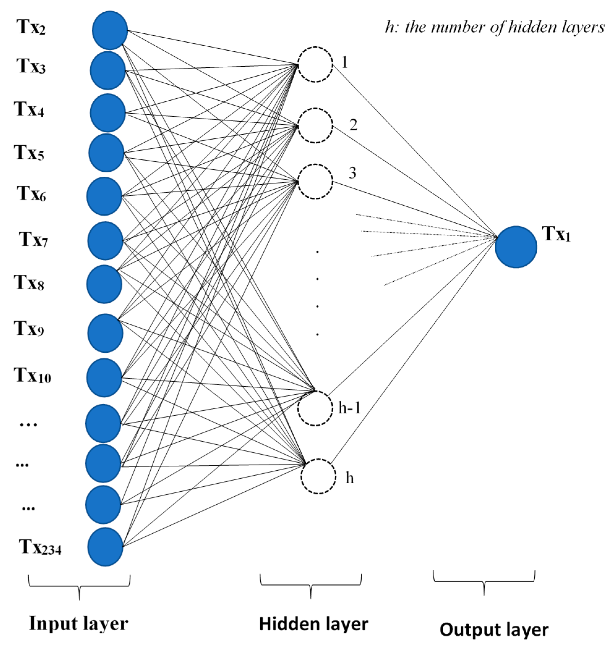
This study used importance scoring to establish the influences of the source components (input data) on the target component’s (output data) behavior. This procedure was meant to determine actionable data processing size that will have an effective contribution to the behavior of the target component. Hence, the first step in the predictive analytics was to correlate the readings of the source components with that of the target component and the cumulative influence of the source components on the target component recorded. The ANN model training, which estimated the value of the target component using the combination of the information in Equations (1)–(3), was carried out using the architecture shown in Figure 3 in a cross-validation ensemble procedure.

Cross-Validation Ensemble

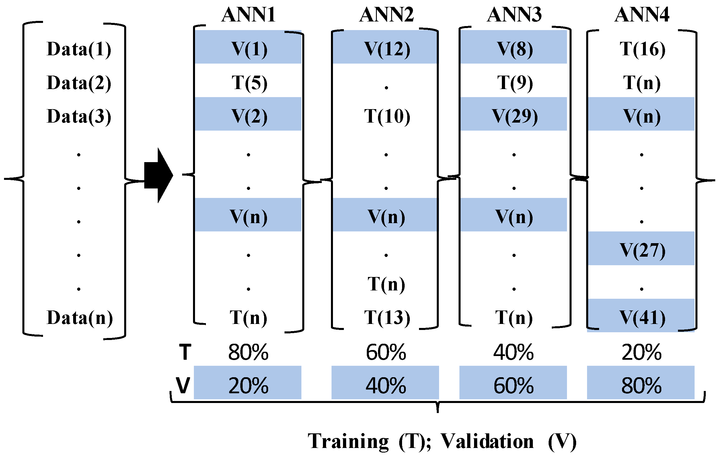
Since this study aims to make a prediction of the future status of the target component from a given set of historic data, a four-fold cross-validation ensemble (Figure 4) that used randomization to pick the validation data from the original dataset was adopted. It can be recalled that this technique has the advantage of considering all sections of the dataset in the training and validation, thereby giving room for robust prediction when compared to the classic approach that uses a given fraction of the data for training and validation. Again, this technique is necessary for reducing variabilities in prediction results and minimizing the chances of type III error, which results in the wrong hypothesis, due to erroneous conclusions [38]. By randomly choosing 20%, 40%, 60% and 80% of the original dataset at separate occasions as the validation dataset and using the remainder as the training dataset, the ANN models were trained. The networks were built with a Multi-Layer Perceptron (MLP) algorithm in a backward propagation technique, by applying grid search to determine the best-trained network amongst different networks having various hidden neurons and learning rates. The varying hidden neurons (H_n) were computed with the expression in Equation (4), by considering the number of input variables (n_col) in the datasets, because preliminary analysis showed that the trained networks with the values obtained from the equation produced high precision results. The learning rates used for the training of the networks were 0.01, 0.15 and 0.25.

$$H_n=\{\begin{array}{c}2n_{col}+1\\ 2n_{col}+2\\ 2n_{col}+3\end{array}$$

(4)

5. Illustrative Example and Results

The cross-validation ensemble ANN technique described in the previous section was exemplified by analyzing 100 days of SCADA sensors’ streamed data of 233 source components that were responsible for the status of one target component (

Table 1. Descriptive statistics of some of the SCADA data used for the analysis (Std.: Standard deviation, COV: Coefficient of Variation).

Descript.	Tx_1	Tx_3	Tx_18	Tx_37	Tx_94	Tx_160	Tx_197	Tx_216	Tx_232	Tx_234
min	0.0000	1.9998	0.0000	9.6552	0.0000	0.0000	0.0000	0.0000	1.9998	0.0000
max	1.9247	8.1290	912.8352	100.0000	99.9546	1.0000	100.0000	1199.7422	8.1979	912.8352
range	1.9247	6.1292	912.8352	90.3448	99.9546	1.0000	100.0000	1199.7422	6.1981	912.8352
median	0.0269	7.4863	487.3383	40.0000	31.6343	0.0000	13.5617	600.0000	7.6996	487.3383
mean	0.2230	7.4596	362.3406	53.4006	24.4100	0.2227	11.5449	514.5615	7.6864	362.3406
Std.	0.4188	0.2081	308.2417	25.5838	23.5495	0.4069	6.9333	282.3706	0.2626	308.2417
COV	1.8778	0.0279	0.8507	0.4791	0.9647	1.8275	0.6006	0.5488	0.0342	0.8507

). This dataset (experimental data), which belongs to a haul crane, is vital for decision-making on the expected status of the target component in the future.

The ANN analysis was done at various levels of the Cumulative Target-component Percentage-influence (CTP)—95.5%, 99.3%, 99.9% and 100%—by using the source components responsible for the CTP levels for the network training. This was done to estimate the actionable size of the source components that will provide the best-trained network at reduced time and cost. It should be noted that the Cumulative Target-component Percentage-influence (CTP) was used to describe the measured cumulative influence of the source components on the target component.

Table 2. Cumulative Target-component Percentage-influence (CTP) and the number of contributing source components.

CTP	Number of Source Components
95.50%	10
99.30%	27
99.90%	46
100%	82

summarizes the number of source components responsible for the various levels of target component behavior after preprocessing the original dataset.

The aggregates of the ANN results obtained at each of the CTP levels—95.5%, 99.3%, 99.9% and 100%—were found by calculating the averages of the built ANN models—ANN1, ANN2, ANN3 and ANN4 (Figure 4)—at the levels. After trying between 1000 and 5000 iterations of the ANN training networks, the best networks from each CTP level was used to compute the Hit Ratio (HR), Miss Ratio (MR), Mean Square Error (MSE) and the coefficient of determination (R²) of the trained and validation datasets per Equations (5)–(7) [39].

$$\{\begin{array}{l}HR=\frac{N_{WF}}{N_s}\\ MR=1-HR\end{array}$$

(5)

$$MSE=\frac{1}{N_s}{\displaystyle \sum }_{i=1}^{N_s}{\left(T_f-T_p\right)}^2$$

(6)

$$R^2=\frac{{\left[{{\displaystyle \sum }}_{i=1}^{N_s}\left\{\left(T_f-T_{mf}\right)\ast \left(T_p-T_{mp}\right)\right\}\right]}^2}{{{\displaystyle \sum }}_{i=1}^{N_s}{\left(T_f-T_{mf}\right)}^2 \ast {{\displaystyle \sum }}_{i=1}^{N_s}{\left(T_p-T_{mp}\right)}^2}$$

(7)

Here, N_WF is the number of the accurately predicted status of the target component over a given number of sampling size N_s, T_f is the original sensor reading, T_p is the ANN predicted sensor reading, T_mp is the mean predicted sensor reading and T_mf is the mean original sensor reading.

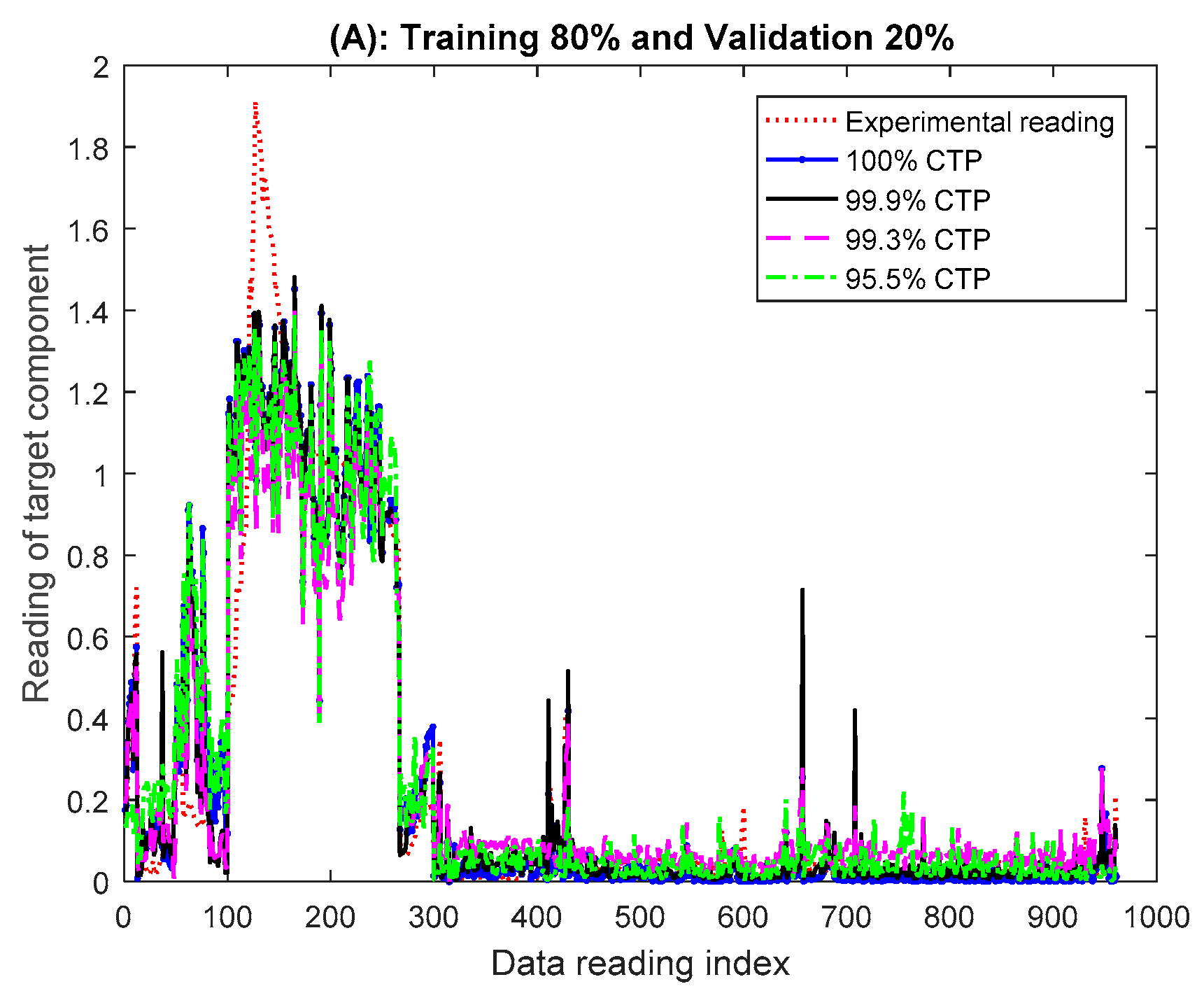
Figure 5 and Figure 6 show the validation results of the cross-validation ensemble ANN at the various CTP levels in comparison to the experimental readings of the target component obtained from the SCADA streamed dataset. Please note that the results for 80% training and 20% validation were used to exemplify the nature of the results obtained from the ANN models. The differences in the results obtained from the ANN models and the experimental results as measured with the Root Mean Square Error (RMSE) are as follows:

-

80% training and 20% validation {100% CTP: 0.0359, 99.9% CTP: 0.0483, 99.3% CTP: 0.0565 and 95.5% CTP:0.0484}

-

60% training and 40% validation {100% CTP: 0.0419, 99.9% CTP:0.0393, 99.3% CTP:0.0386 and 95.5% CTP:0.050}

-

40% training and 60% validation {100% CTP: 0.044, 99.9% CTP: 0.0365, 99.3% CTP: 0.0391 and 95.5% CTP: 0.0515}

-

20% training and 80% validation {100% CTP: 0.0455, 99.9% CTP: 0.0384, 99.3% CTP: 0.0407 and 95.5% CTP: 0.093}.

The correlation of the cross-validation ensemble ANN predicted target component readings and the experimental results shown in Figure 6 as determined with Equations (5)–(7) are summarized in

Table 3. Summary of the best-trained networks, R², Mean Square Error (MSE), Hit Ratio (HR) and Miss Ratio (MR) for various Cumulative Target-component Percentage-influence (CTP).

TD:VD (%)	Training Dataset (TD)		Validation Dataset (VD)				CTP
	R2	MSE	R2	MSE	HR	MR
80:20	0.856	0.0254	0.848	0.0277	90.53%	9.47%	95.50%
60:40	0.852	0.0266	0.839	0.0282	90.53%	9.47%
40:60	0.836	0.0301	0.833	0.0289	91.88%	8.12%
20:80	0.87	0.0236	0.862	0.0289	89.87%	10.13%
Average	0.853	0.0264	0.845	0.0284	90.70%	9.30%
80:20	0.886	0.0224	0.878	0.0245	94.59%	5.41%	99.30%
60:40	0.886	0.0211	0.877	0.0227	92.19%	7.81%
40:60	0.884	0.0214	0.881	0.0204	94.86%	5.14%
20:80	0.889	0.0176	0.876	0.0232	93.65%	6.35%
Average	0.886	0.021	0.878	0.023	93.80%	6.18%
80:20	0.89	0.0192	0.881	0.0216	94.69%	5.31%	99.90%
60:40	0.889	0.021	0.879	0.0216	95.26%	4.74%
40:60	0.887	0.0214	0.881	0.0205	96.18%	3.82%
20:80	0.889	0.0176	0.876	0.0233	94.85%	5.15%
Average	0.889	0.02	0.879	0.022	95.20%	4.76%
80:20	0.881	0.0208	0.873	0.023	94.38%	5.62%	100%
60:40	0.887	0.0201	0.877	0.0212	94.12%	5.88%
40:60	0.879	0.0227	0.877	0.0226	94.59%	5.41%
20:80	0.884	0.0175	0.869	0.0238	94.87%	5.13%
Average	0.883	0.02	0.874	0.023	94.50%	5.51%

.

It can be inferred from the results (Table 3) that the 99.9% CTP level ANN model (validation dataset) is the best model for estimating the degradation of the target component, with an average hit ratio of 95.20%, which is 0.7%, 1.4% and 4.5% better than the hit ratios at the 100%, 99.3% and 95.5% CTP levels, respectively. Similarly, the coefficient of determination (R²) for the 99.9% CTP level is also higher than those of the other CTP levels. The higher explanatory power and accuracy of the prediction at the 99.9% CTP level, compared to the 100% CTP level, could be because of the very low influences {0.000%–0.0007%} of the input variables that succeeded the 99.9% CTP level have on the behavior of the target component.

Comparison of Cross-Validation Ensemble ANN with Classic ANN and other Techniques

For comparing the cross-validation ensemble technique of ANN used in this study with the classic ANN used by other researchers on fault detection and diagnostics of industrial assets [40,41,42], the dataset used for this study was subjected to a classic ANN (70% training and 30% validation).

Table 4. Comparison of classic ANN and the cross-validation ensemble technique.

CTP	Classic ANN Dataset (70% Training, 30% Validation)		Cross-Validation Ensemble ANN
	Hit Ratio (HR)	Miss Ratio (MR)	Hit Ratio (HR)	Miss Ratio (MR)
95.50%	89.45%	10.55%	90.7%	9.3%
99.30%	91.95%	8.05%	93.8%	6.18%
99.90%	94.10%	5.90%	95.2%	4.76%
100%	93.89%	6.11%	94.5%	5.51%

shows the comparison of both results. Judging from the HR and MR obtained from both techniques (Table 4), it can be inferred that the cross-validation ensemble technique has obvious advantages over the classic ANN, due to its ability to make more accurate estimations compared to the classic ANN.

The cross-validation ensemble ANN was also compared with other fault detection techniques to affirm the robustness of the technique.

Table 5. Comparison of the performance of different fault detection and identification techniques with Cross-Validation Ensemble ANN (CVEANN).

Technique	Accuracy	Variation from CVEANN	Ref
ANN (classic)	95%	−0.20%	[43]
Artificial Neural Network with Particle Swarm Optimization (ANN-PSO)	96%	0.80%	[43]
Artificial Neural Network with Iterative Particle Swarm Optimization (ANN-IPSO)	97%	1.80%	[43]
Artificial Neural Network with Evolutionary Particle Swarm Optimization (ANN-EPSO)	98%	2.80%	[43]
Evolutionary Programming Artificial Neural Network (EPANN)	95%	−0.20%	[44]
Fussy logic	89%	−6.20%	[45]
Rough set theory	92.11%	−3.09%	[46]
Support Vector Machine (SVM)	92%	−3.20%	[47]
Phase editing	79%	−16.20%	[22]
Cepstral editing	69%, 72%	−26.2%, −23.2%	[48,49]
Artificial Neural Network with Expert System (ANN-EPS)	90.40%	−4.8%	[50]
Bootstrap Genetic Programming and K-Nearest Neighbor (GP-KNN)	92.11%	−3.09%	[51]

summarizes the methods and the level of accuracy obtained using them. It can be inferred from this table that cross-validation ensemble ANN with the prediction accuracy of 95.2% outperformed classic ANN, Evolutionary Programming ANN (EPANN), fuzzy logic, immune neural network, rough set theory, SVM, bootstrap and Genetic Programming with K-Nearest Neighbors (GP-KNN), phase editing and cepstral editing, whereas ANN-PSO, ANN-IPSO, ANN with Evolutionary Particle Swarm Optimization (ANN-EPSO) performed better than the cross-validation ensemble ANN. To further improve on the Cross-Validation Ensemble Artificial Neural Network (CVEANN) to enhance the accuracy of the predictions, it may be necessary to increase the number of validation folds from four to between eight and twelve, as this will make it possible to consider smaller fractions of the dataset and could improve the prediction accuracy.

6. Predicting Future Behavior of the Target Component

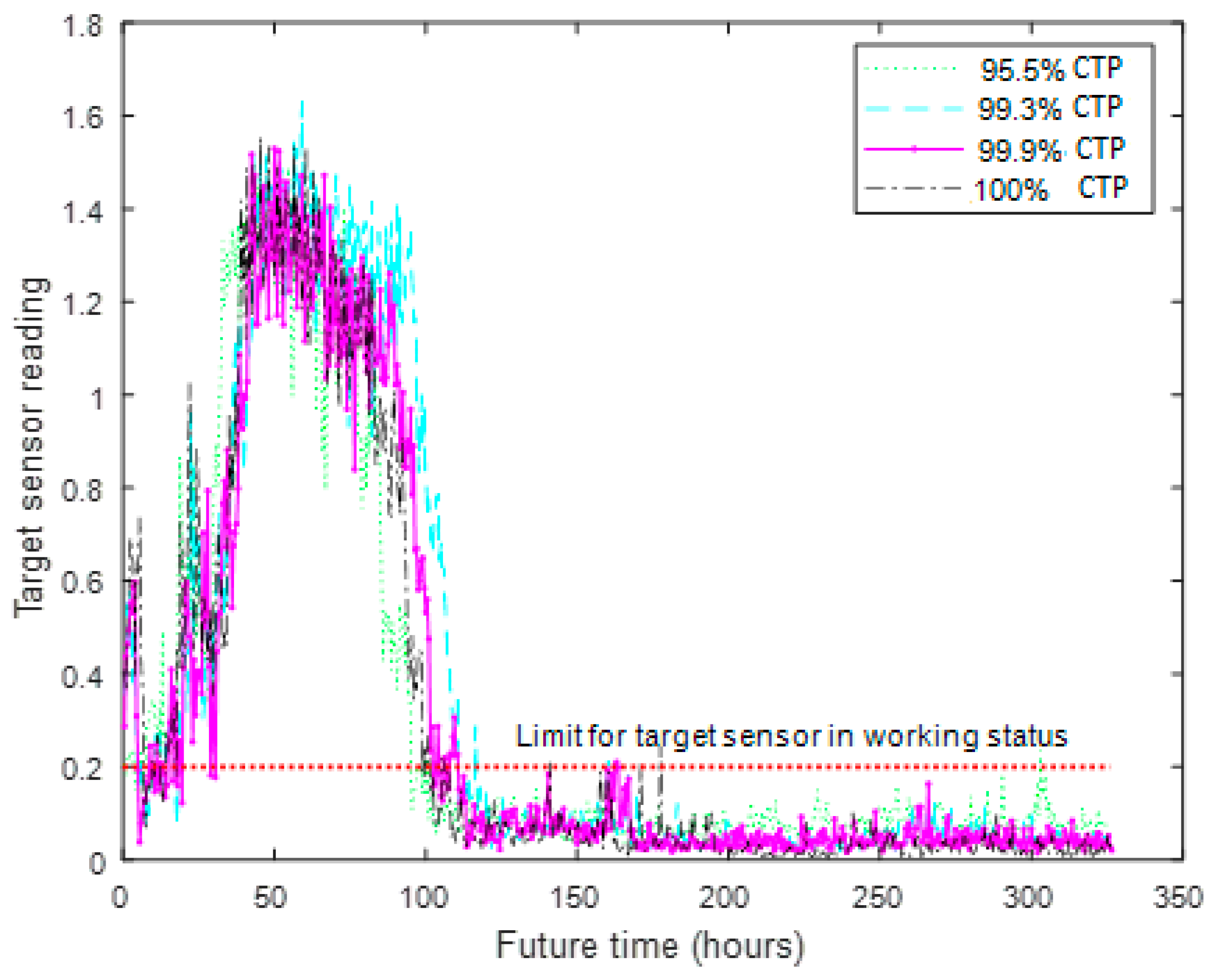
The best results of the trained networks were used for the estimation of the future state of the target component by randomly generating readings from the original dataset (source components). These readings were subjected to measurement noises that were assumed to cause the readings to fluctuate randomly between ±2.5%. The summarized results of the average future target sensor readings at the CTP levels are shown in Figure 7. Since the 99.9% CTP level gave the best estimation of the validation dataset of the target component, the expected future status of the target component was computed with the model. The summary of the target sensor behavior in the future 358 h (~15 days) using the 99.9% CTP level is shown in

Table 6. Expected future status of the target component, the date and time the fault is expected, the duration of the fault and the requisite maintenance action required for the source components.

Date/Time (Start)	Date/Time (End)	Duration (h)	System Status	Required Maintenance	Duration (h)	System Status	Required Maintenance
16 May 2016 9:30	16 May 2016 1:30	4.00	faulty	minor	0.5–4.5	faulty	minor
16 May 2016 14:00	16 May 2016 17:30	3.50	working		5–8.5	working
16 May 2016 18:00	16 May 2016 18:00	0.50	faulty	minor	9	faulty	minor
16 May 2016 18:30	16 May 2016 18:30	0.50	working		9.5	working
16 May 2016 19:00	16 May 2016 19:00	0.50	faulty	minor	10	faulty	minor
16 May 2016 19:30	16 May 2016 19:30	0.50	working		10.5	working
16 May 2016 20:00	16 May 2016 20:00	0.50	faulty	minor	11	faulty	minor
16 May 2016 20:30	16 May 2016 21:00	1.00	working		11.5–12	working
16 May 2016 21:30	16 May 2016 22:00	1.00	faulty	minor	12.5–13	faulty	minor
16 May 2016 22:30	16 May 2016 23:30	1.50	working		13.5–14.5	working
17 May 2016 0:00	17 May 2016 1:00	1.00	faulty	minor	15–16	faulty	minor
17 May 2016 1:30	17 May 2016 1:30	0.50	working		16.5	working
17 May 2016 2:00	17 May 2016 2:30	1.00	faulty	minor	17–17.5	faulty	minor
17 May 2016 3:00	17 May 2016 3:00	0.50	working		18	working
17 May 2016 3:30	17 May 2016 4:00	1.00	faulty	minor	18.5–19	faulty	minor
17 May 2016 4:30	17 May 2016 4:30	0.50	working		19.5	working
17 May 2016 5:00	17 May 2016 13:30	8.50	faulty	major	20–28.5	faulty	major
17 May 2016 14:00	17 May 2016 14:00	0.50	working		29	working
17 May 2016 14:30	17 May 2016 15:00	1.00	faulty	minor	29.5–30	faulty	minor
17 May 2016 15:30	17 May 2016 15:30	0.50	working		30.5	working
17 May 2016 16:00	20 May 2016 15:00	71.00	faulty	shutdown	31–102	faulty	shutdown
20 May 2016 15:30	20 May 2016 16:00	1.00	working		102.5–103	working
20 May 2016 16:30	20 May 2016 17:00	1.00	faulty	minor	103.5–104	faulty	minor
20 May 2016 17:30	20 May 2016 18:30	1.50	working		104.5–105.5	working
20 May 2016 21:00	20 May 2016 23:30	3.50	faulty	minor	108–110.5	faulty	minor
21 May 2016 0:00	23 May 2016 3:30	51.50	working		111–162.5	working
23 May 2016 4:00	23 May 2016 4:00	0.50	faulty	minor	163	faulty	minor
23 May 2016 4:30	31 May 2016 7:00	194.50	working		163.5–358	working

. The future readings of the target component (Table 6) form the basis for decision-making on the time faults are to be expected and the requisite actions to be taken. Hence, when the target component is expected to have a faulty status that will last for less than four hours, the maintenance will be expected to be a minor one and could involve replacement of fuses and resetting of relays. However, when the future time of failure is expected to last for 4–16 h consecutively, a major maintenance will be planned. This category of maintenance may warrant fault isolation at the sub-system levels and requires higher specialty of technical personnel in comparison to minor maintenance operations. Similarly, when the expected future faulty status of the target component goes above 16 h consecutively, a shutdown maintenance is anticipated, because some critical components, such as the bearings, shafts, rollers etc., will either need replacement or servicing, due to deteriorations that could involve deformation, fatigue failure, cracking and corrosion damages.

Following the explanatory power of the 99.9% CTP level used for the prediction of the future behavior of the target component, it could be expected that approximately 13% variability in the expected time of failure and duration of the faulty status of the target component may occur. To this end, contingency actions could be taken ahead of time to prevent the disruption of operations, by planning maintenance in advance, shifting workforce to other machinery and stopping operation of assets that have been predicted to breakdown, which could help to prevent more damages to the assets and reduce the operating cost. Incorporating this prediction model into an integrated asset management architecture will provide a module for automated fault detection and identification, which will help to improve the integrity of assets.

7. Conclusions

The implementation of intelligent asset integrity management has been made easier by big data of components’ degradations obtained over the years of service of the facilities. The utilization of these assets’ condition monitoring indicators for decision making on the future status of the components of the assets has made it possible to have real-time fault detection, identification and cost-effective maintenance management. This study has utilized cross-validation ensemble ANN for a predictive analytic study that aimed at estimating the future status of a target component that was influenced by the source components in a complex system of a haul crane. A four-fold randomized selection of the population of the original dataset was done using 20% training and 80% validation, 40% training and 60% validation, 60% training and 40% validation and 80% training and 20% validation at different moments of the ANN modeling. The study implemented importance scoring to determine the influence of the source components on the output component and used the number of source components that contributed to 95.5%, 99.3%, 99.9% and 100% of the target component behavior to carry out the ANN network trainings at different instances. After comparing the validation results at the Cumulative Target-component Percentage-influence (CTP) levels of 95.5%, 99.3%, 99.9% and 100%, it was observed that the 99.9% CTP level with the coefficient of determination (R²) of 0.879, hit ratio of 95.2% and miss ratio of 4.76% was the best network for making the prediction of the status of the haul crane components used as a case study in this work.

The study also compared the cross-validation ensemble ANN technique with the best prediction accuracy (99.9% CTP level) with the classical ANN and other machine learning tools that have been employed in the literature to predict the faults of complex systems. It was observed that the technique used in this study could more accurately predict the system’s behavior than classic ANN, EPANN, fuzzy logic, immune neural network, rough set theory, SVM, GP-KNN, phase editing and cepstral editing. On the other hand, the ANN-PSO, ANN-IPSO and ANNEPSO techniques predicted the system’s performance more accurately than the cross-validation ensemble ANN employed in this study.

Finally, the 99.9% CTP level cross-validation ensemble ANN was used to predict the future state of the target component of the haul crane, and the results were used to envisage the expected time of the system breakdown and the type of maintenance that will be probable. It is expected that future studies on the complex systems will focus on using 8–12-fold cross-validation ensemble ANN with particle swarm optimization and evolution-based modifications to improve the accuracy of the predictions.

References

- Lee, J.; Ni, J.; Djurdjanovic, D.; Qiu, H.; Liao, H. Intelligent prognostics tools and e-maintenance. Comput. Ind. 2006, 57, 476–489. [Google Scholar] [CrossRef]
- Yam, R.C.M.; Tse, P.W.; Li, L.; Tu, P. Intelligent predictive decision support system for condition-based maintenance. Int. J. Adv. Manuf. Technol. 2001, 17, 383–391. [Google Scholar] [CrossRef]
- Montgomery, R.L.; Serratella, C. Risk-based maintenance: A new vision for asset integrity management. In Proceedings of the ASME 2002 Pressure Vessels and Piping Conference, Vancouver, BC, Canada, 5–9 August 2002; American Society of Mechanical Engineers: New York, NY, USA, 2002; pp. 151–165. [Google Scholar]
- Mohanty, S.; Jagadeesh, M.; Srivatsa, H. Big Data Imperatives: Enterprise ‘Big Data’ Warehouse, ‘BI’ Implementations and Analytics; Apress: New York, NY, USA, 2013. [Google Scholar]
- Ratnayake, R.C. Modelling of asset integrity management process: A case study for computing operational integrity preference weights. Int. J. Comput. Syst. Eng. 2012, 1, 3–12. [Google Scholar] [CrossRef]
- Rastegari, A.; Mobin, M. Maintenance decision making, supported by computerized maintenance management system. In Proceedings of the 2016 IEEE Annual Reliability and Maintainability Symposium (RAMS), Tucson, AZ, USA, 25–28 January 2016; pp. 1–8. [Google Scholar]
- Misra, K.B. Maintenance engineering and maintainability: An introduction. In Handbook of Performability Engineering; Springer: London, UK, 2008; pp. 755–772. [Google Scholar]
- Shafiee, M.; Finkelstein, M. An optimal age-based group maintenance policy for multi-unit degrading systems. Reliab. Eng. Syst. Saf. 2015, 134, 230–238. [Google Scholar] [CrossRef]
- Boone, C.A.; Skipper, J.B.; Hazen, B.T. A framework for investigating the role of big data in service parts management. J. Clean. Prod. 2017, 153, 687–691. [Google Scholar] [CrossRef]
- Daneshkhah, A.; Hosseinian-Far, A.; Chatrabgoun, O. Sustainable Maintenance Strategy Under Uncertainty in the Lifetime Distribution of Deteriorating Assets. In Strategic Engineering for Cloud Computing and Big Data Analytics; Springer: Cham, Swizerland, 2017; pp. 29–50. [Google Scholar]
- Lapworth, J.A.; Wilson, A. The asset health review for managing reliability risks associated with ongoing use of ageing system power transformers. In Proceedings of the CMD 2008 IEEE International Conference on Condition Monitoring and Diagnosis, Beijing, China, 21–24 April 2008; pp. 605–608. [Google Scholar]
- Remy, E.; Corset, F.; Despréaux, S.; Doyen, L.; Gaudoin, O. An example of integrated approach to technical and economic optimization of maintenance. Reliab. Eng. Syst. Saf. 2013, 116, 8–19. [Google Scholar] [CrossRef]
- Volovoi, V.; Valenzuela, R.C. On compact modeling of coupling effects in maintenance processes of complex systems. Int. J. Eng. Sci. 2012, 59, 193–210. [Google Scholar] [CrossRef]
- Carlos, S.; Sánchez, A.; Martorell, S.; Villanueva, J.F. Particle Swarm Optimization of safety components and systems of nuclear power plants under uncertain maintenance planning. Adv. Eng. Softw. 2012, 50, 12–18. [Google Scholar] [CrossRef]
- Guo, C.; Wang, W.; Guo, B.; Si, X. A maintenance optimization model for mission-oriented systems based on Wiener degradation. Reliab. Eng. Syst. Saf. 2013, 111, 183–194. [Google Scholar] [CrossRef]
- Aven, T.; Castro, I.T. A delay-time model with safety constraint. Reliab. Eng. Syst. Saf. 2009, 94, 261–267. [Google Scholar] [CrossRef]
- Wang, W. A stochastic model for joint spare parts inventory and planned maintenance optimization. Eur. J. Oper. Res. 2012, 216, 127–139. [Google Scholar] [CrossRef]
- Baker, R.D.; Christer, A.H. Review of delay-time OR modelling of engineering aspects of maintenance. Eur. J. Oper. Res. 1994, 73, 407–422. [Google Scholar] [CrossRef]
- Kan, M.S.; Tan, A.C.C.; Mathew, J. A review on prognostic techniques for non-stationary and non-linear rotating systems. Mech. Syst. Signal Process. 2015, 62–63, 1–20. [Google Scholar] [CrossRef]
- Nabati, E.G.; Thoben, K.-D. Data Driven Decision Making in Planning the Maintenance Activities of Off-shore Wind Energy. Procedia CIRP 2017, 59, 160–165. [Google Scholar] [CrossRef]
- Fumeo, E.; Oneto, L.; Anguita, D. Condition Based Maintenance in Railway Transportation Systems Based on Big Data Streaming Analysis. Procedia Comput. Sci. 2015, 53, 437–446. [Google Scholar] [CrossRef]
- Barbini, L.; Ompusunggu, A.P.; Hillis, A.J.; du Bois, J.L.; Bartic, A. Phase editing as a signal pre-processing step for automated bearing fault detection. Mech. Syst. Signal Process. 2017, 91, 407–421. [Google Scholar] [CrossRef]
- Kumar, A.; Shankar, R.; Thakur, L.S. A big data driven sustainable manufacturing framework for condition-based maintenance prediction. J. Comput. Sci. 2017. [Google Scholar] [CrossRef]
- Manco, G.; Ritacco, E.; Rullo, P.; Gallucci, L.; Astill, W.; Kimber, D.; Antonelli, M. Fault detection and explanation through big data analysis on sensor streams. Expert Syst. Appli. 2017, 87, 141–156. [Google Scholar] [CrossRef]
- Cai, J.; Cottis, R.A.; Lyon, S.B. Phenomenological modelling of atmospheric corrosion using an artificial neural network. Corros. Sci. 1999, 41, 2001–2030. [Google Scholar] [CrossRef]
- Wang, S.C. Artificial neural network. In Interdisciplinary Computing in Java Programming; Springer: New York, NY, USA, 2003; pp. 81–100. [Google Scholar]
- Wang, P.; Vachtsevanos, G. Fault prognostics using dynamic wavelet neural networks. AI EDAM 2001, 15, 349–365. [Google Scholar] [CrossRef]
- Horrocks, P.; Mansfield, D.; Parker, K.; Thomson, J.; Atkinson, T.; Worsley, J.; House, W.; Park, B. Managing Ageing Plant; Technical Report; HSE: Warrington, UK, 2010; Volume 823.
- Lee, J.; Wu, F.; Zhao, W.; Ghaffari, M.; Liao, L.; Siegel, D. Prognostics and health management design for rotary machinery systems—Reviews, methodology and applications. Mech. Syst. Signal Process. 2014, 42, 314–334. [Google Scholar] [CrossRef]
- Peng, Y.; Dong, M.; Zuo, M.J. Current status of machine prognostics in condition-based maintenance: A review. Int. J. Adv. Manuf. Technol. 2010, 50, 297–313. [Google Scholar] [CrossRef]
- Joly, R.B.; Ogaji, S.O.T.; Singh, R.; Probert, S.D. Gas-turbine diagnostics using artificial neural-networks for a high bypass ratio military turbofan engine. Appl. Energy 2004, 78, 397–418. [Google Scholar] [CrossRef] [Green Version]
- Schwabacher, M. A survey of data-driven prognostics. In Infotech@ Aerospace; Mark Schwabacher, NASA Ames Research Center: Arlington, VA, USA, 2005; p. 7002. [Google Scholar]
- Kothamasu, R.; Huang, S.H.; VerDuin, W.H. System health monitoring and prognostics—A review of current paradigms and practices. In Handbook of Maintenance Management and Engineering; Springer: London, UK, 2009; pp. 337–362. [Google Scholar]
- Van Oosterom, C.D.; Elwany, A.H.; Çelebi, D.; Van Houtum, G.J. Optimal policies for a delay time model with postponed replacement. Eur. J. Oper. Res. 2014, 232, 186–197. [Google Scholar] [CrossRef]
- Christer, A.H.; Lee, C.; Wang, W. A data deficiency based parameter estimating problem and case study in delay time PM modeling. Int. J. Prod. Econ. 2000, 67, 63–76. [Google Scholar] [CrossRef]
- Wang, W.; Banjevic, D.; Pecht, M. A multi-component and multi-failure mode inspection model based on the delay time concept. Reliab. Eng. Syst. Saf. 2010, 95, 912–920. [Google Scholar] [CrossRef]
- Dietterich, T. Overfitting and under computing in machine learning. ACM Comput. Surv. (CSUR) 1995, 27, 326–327. [Google Scholar] [CrossRef]
- Donate, J.P.; Cortez, P.; Sanchez, G.G.; De Miguel, A.S. Time series forecasting using a weighted cross-validation evolutionary artificial neural network ensemble. Neurocomputing 2013, 109, 27–32. [Google Scholar] [CrossRef] [Green Version]
- Abyaneh, H.Z. Evaluation of multivariate linear regression and artificial neural networks in prediction of water quality parameters. J. Environ. Health Sci. Eng. 2014, 12, 40. [Google Scholar] [CrossRef] [PubMed]
- Garcia, M.C.; Sanz-Bobi, M.A.; del Pico, J. SIMAP: Intelligent system for predictive maintenance: Application to the health condition monitoring of a windturbine gearbox. Comput. Ind. 2006, 57, 552–568. [Google Scholar] [CrossRef]
- Zaher, A.; McArthur, S.D.J.; Infield, D.G.; Patel, Y. Online wind turbine fault detection through automated SCADA data analysis. Wind Energy 2009, 12, 574–593. [Google Scholar] [CrossRef]
- Bangalore, P.; Tjernberg, L.B. An artificial neural network approach for early fault detection of gearbox bearings. IEEE Trans. Smart Grid 2015, 6, 980–987. [Google Scholar] [CrossRef]
- Illias, H.Z.; Chai, X.R.; Mokhlis, H. Transformer incipient fault prediction using combined artificial neural network and various particle swarm optimisation techniques. PLoS ONE 2015, 10, e0129363. [Google Scholar] [CrossRef] [PubMed]
- Zakaria, F.; Johari, D.; Musirin, I. Optimized Artificial Neural Network for the detection of incipient faults in power transformer. In Proceedings of the 2014 IEEE 8th International Power Engineering and Optimization Conference (PEOCO), Langkawi, Malaysia, 24–25 March 2014; pp. 635–640. [Google Scholar]
- Ahmed, M.R.; Geliel, M.A.; Khalil, A. Power transformer fault diagnosis using fuzzy logic technique based on dissolved gas analysis. In Proceedings of the 2013 IEEE 21st Mediterranean Conference on Control & Automation (MED), Chania, Greece, 25–28 June 2013; pp. 584–589. [Google Scholar]
- Setiawan, N.A.; Adhiarga, Z. Power transformer incipient faults diagnosis using Dissolved Gas Analysis and Rough Set. In Proceedings of the 2012 IEEE International Conference on Condition Monitoring and Diagnosis (CMD), Bali, Indonesia, 23–27 September 2012; pp. 950–953. [Google Scholar]
- Yang, H.T.; Huang, Y.C. Intelligent decision support for diagnosis of incipient transformer faults using self-organizing polynomial networks. IEEE Trans. Power Syst. 1998, 13, 946–952. [Google Scholar] [CrossRef]
- Antoni, J. The spectral kurtosis: A useful tool for characterising non-stationary signals. Mech. Syst. Signal Process. 2006, 20, 282–307. [Google Scholar] [CrossRef]
- Borghesani, P.; Pennacchi, P.; Randall, R.; Sawalhi, N.; Ricci, R. Application of cepstrum pre-whitening for the diagnosis of bearing faults under variable speed conditions. Mech. Syst. Signal Process. 2013, 36, 370–384. [Google Scholar] [CrossRef]
- Wang, Z.; Liu, Y.; Griffin, P.J. A combined ANN and expert system tool for transformer fault diagnosis. IEEE Trans. Power Deliv. 1998, 13, 1224–1229. [Google Scholar] [CrossRef]
- Shintemirov, A.; Tang, W.; Wu, Q.H. Power transformer fault classification based on dissolved gas analysis by implementing bootstrap and genetic programming. IEEE Trans. Syst. Man Cybern. Part C Appl. Rev. 2009, 39, 69–79. [Google Scholar] [CrossRef]
Figure 1.
Framework for intelligent prognosis of complex systems (Note: SCADA, Supervisory Control And Data Acquisition; CMS, Condition Monitoring Sensor; ANN, Artificial Neural Network; SVM, Support Vector Machine; GBM, Gradient Boosting Machine; RF, Random Forest; DL, Deep Learning; GS, Grid Search; GLM, Generalized Linear Model; SMPP, Statistical Matching Performance Pattern).
Figure 2.
Integrated process of fault detection and identification with Artificial Neural Networks (ANNs).
Figure 3.
ANN architecture used for the model development, Tx1 is the target component (output) and Tx2, Tx3, …, Tx234 represent the source components (inputs) of the system.
Figure 4.
A randomization based four-fold cross-validation ensemble used for the ANN training and validation of the dataset.
Figure 5.
Comparison of the experimental and the cross-validation ensemble ANN predicted target sensor readings for the 95%, 99.3%, 99.9% and 100% levels of the Cumulative Target-component Percentage-influence (CTP) of the validation dataset.
Figure 6.
Performance evaluation of the experimental data with the predictions of the cross-validation ensemble ANN at the 95%, 99.3%, 99.9% and 100% levels of the Cumulative Target-component Percentage-influence (CTP) of the validation dataset.
Figure 7.
Comparison of the cross-validation ensemble ANN modeled future target sensor reading for the 95.5%, 99.3%, 99.9% and 100% CTP levels.