Forecasting Net Income Estimate and Stock Price Using Text Mining from Economic Reports
by
 , , and
Masahiro Suzuki
1,* ,
,
Hiroki Sakaji
1,
Kiyoshi Izumi
1,
Hiroyasu Matsushima
1 and
Yasushi Ishikawa
2 1
Department of Systems Innovation, School of Engineering, The University of Tokyo, Tokyo 113-8656, Japan
2
Nikko Asset Management Co., Ltd., Tokyo 107-6242, Japan
*
Author to whom correspondence should be addressed.
Information 2020, 11(6), 292; https://doi.org/10.3390/info11060292
Submission received: 30 April 2020
/
Revised: 17 May 2020
/
Accepted: 27 May 2020
/
Published: 30 May 2020
(This article belongs to the Special Issue CDEC: Cross-disciplinary Data Exchange and Collaboration)
Abstract
:This paper proposes and analyzes a methodology of forecasting movements of the analysts’ net income estimates and those of stock prices. We achieve this by applying natural language processing and neural networks in the context of analyst reports. In the pre-experiment, we applied our method to extract opinion sentences from the analyst report while classifying the remaining parts as non-opinion sentences. Then, we performed two additional experiments. First, we employed our proposed method for forecasting the movements of analysts’ net income estimates by inputting the opinion and non-opinion sentences into separate neural networks. Besides the reports, we inputted the trend of the net income estimate to the networks. Second, we employed our proposed method for forecasting the movements of stock prices. Consequently, we found differences between security firms, which depend on whether analysts’ net income estimates tend to be forecasted by opinions or facts in the context of analyst reports. Furthermore, the trend of the net income estimate was found to be effective for the forecast as well as an analyst report. However, in experiments of forecasting movements of stock prices, the difference between opinion sentences and non-opinion sentences was not effective.
1. Introduction
According to the Japan Exchange Group’s (JPX) research, the number of individual shareholders is rising in Japan (https://www.jpx.co.jp/markets/statistics-equities/examination/01.html). In particular, the number of individual investors in Japan achieved 49.67 million in 2016 and increased further by 1.62 million in 2017, exceeding 50 million for the first time. The number of individual investors is expected to increase continuously. Recently, the stock prices of most companies have been on the rise due to the effects of Abenomics (Abenomics refers to the economic policies advocated by Japanese Prime Minister Shinzō Abe since the general elections of December 2012) and the Olympics Games scheduled for 2020.
There is a need for investors to examine much information so as to invest in target companies. However, the sources of information are different, and the process of collecting information necessary for investment is complicated. Looking at a company’s website, there are various reports, namely financial statements, financial results’ briefing materials, annual reports, and securities reports, on the investor relations page. If we use a search engine to find a company’s name, we may find different news reports. Moreover, Internet message boards for financial markets include various investors’ opinions related to financial information and stock price movements. Furthermore, in recent years, people’s comments on social networking sites, such as Twitter, Facebook, and Instagram, have been reflecting investor sentiments. Bollen et al. showed that mood states obtained from tweets are relevant for forecasting the Dow Jones Industrial Average (DJIA) [1]. The progress of computation assists us in referring to such information. On the other hand, it is getting difficult for investors to find appropriate information for their investments.
In this environment, it would be interesting to investigate whether the context of analyst reports have predictive power for the future movement of a stock price. An analyst report is referred to as a report written by analysts to evaluate individual companies by considering the following: news, press releases, stock valuations, and macroeconomic trends. Therefore, we consider analyst reports as an upward compatibility of the information sources for each investment. In this study, we analyzed the texts of analyst reports in forecasting trends of stock prices. Particularly, we aimed at forecasting the sign of stock price excess return to the market and the extent of stock price volatility, which are crucial in trends of stock prices.
Furthermore, we classified analyst reports by brokerage company and evaluated their effectiveness for each brokerage company, as the style and content of these reports depend on the company. We applied several word-embedding models developed from various resources. Therefore, we experimented with a variety of different data.
Figure 1 shows the flow of the experiment in this paper. Basically, we performed three experiments. In the first experiment, we formulated a model to extract opinion sentences using 2213 sentences in analyst reports (we refer to these sentences as analyst report sentences). Section 5 discusses this experiment. We consider this as a pre-experiment for the remaining two experiments. The proposed model distinguishes the opinion and non-opinion sentences from the analyst report set, which comprises 17,356 analyst reports. Second, we forecasted the analyst’s revision of the net income estimate using opinion and non-opinion sentences extracted from analyst reports and using trends of the net income estimate. We show this experiment in Section 6.1. Third, we forecasted movements of excess returns and volatilities with opinion and non-opinion sentences. Section 6.2 shows this experiment.
2. Related Works
There are various studies on financial text mining for the prediction of financial markets [2]. Bollen et al. showed that mood states obtained from tweets are relevant for forecasting the DJIA [1]. They applied OpinionFinder and G-POMS to extract seven public moods from tweets. They also applied self-organizing fuzzy neural networks for forecasting, and, consequently, could predict rises and drops with an accuracy of more than 80%. They found that mood states in terms of positive or negative mood are not effective in forecasting but those labeled “Calm” are effective. Schumaker et al. proposed and analyzed a machine-learning method for forecasting stock prices by analyzing financial news articles [3]. Their model forecasted indicators and stock prices by using a resource. Schumaker et al. united their approach using sentiment analysis [4]. They estimated stock prices after releasing financial news articles with SVM. Koppel et al. proposed a method for classifying the news stories of a company according to their apparent impacts on the performance of the company’s stock price [5]. Low et al. proposed a semantic expectation-based knowledge extraction methodology for extracting causal relations by using WordNet as a thesaurus for extracting terms representing movement concepts [6]. Ito et al. proposed a neural network model for visualizing online financial textual data [7,8]. Their proposed model acquired word sentiment and its category. Milea et al. predicted the MSCI euro index (upwards, downwards, or constant) based on fuzzy grammar fragments extracted from a report published by the European Central Bank [9]. Wuthrich et al. predicted daily movements of five indices using news articles published on the Internet [10]. They constructed the rule to predict with a combination of news articles, index values, and some keywords. They found that textual information with bag-of-words in addition to numeric time-series data increases the quality of the input. Bar-Haim et al. proposed a framework for identifying expert investors and used it for predicting stock price rise from stock tweets applying an SVM classifier [11]. They trained the classifier that directly learned the relationship between the content of a tweet and the stock prices. The user who was writing tweets that could discriminate the rise/fall of the stock price was learned as a specialist. Then, they constructed the classifier trained only by the set of tweets of the identified experts. Guijarro et al. analyzed the impact of investors’ mood on market liquidity [12]. They performed sentiment analysis of tweets related to the S&P 500 Index. Vu et al. proposed a method using a Decision Tree classifier to predict the daily price movements of four famous tech stocks [13]. They applied sentiment analysis, semantic orientation (SO), and movements of previous days as features for tweets. They predicted with an accuracy of more than 75%. Oliveira et al. constructed sentiment and attention indicators extracted from microblogs and then utilized machine learning-based methods for financial tweets sentiment classification of predicting daily stock market variables [14]. They tested five machine learning-based methods for financial tweets sentiment classification with the indicators. Zhang et al. proposed a context-aware deep embedding network to detect financial opinions behind texts extracted from Twitter [15]. They jointly learned and exploited user embeddings and the texts. Ranco et al. analyzed the effects of sentiments of tweets about companies on DJIA 30 prices applying SVM [16]. They found a dependence between stock price returns and Twitter sentiments. Smailović et al. showed causality between sentiment polarity of tweets and daily return of closing prices [17]. The authors also applied sentiment derived from an SVM model to classify the tweets into positive, negative, and neutral categories. Our proposed method uses a combination of several documents, such as analyst reports and the Wikipedia corpus, for forecasting stock price movements.
Regarding financial text mining for the Japanese language, Sakaji et al. proposed a method to automatically extract basis expressions that indicate economic trends from newspaper articles using a statistical method [18]. In addition, Sakaji et al. proposed an unsupervised approach to discover rare causal knowledge from financial statement summaries [19]. Their method extracted basis expressions and causal knowledge using syntactic patterns. Kitamori et al. proposed a method for extracting and classifying sentences indicating business performance forecasts and economic forecasts from summaries of financial statements [20]. This classification method was based on a neural network using a semi-supervised approach. Hirano et al. proposed a generalized scheme for selecting related stocks for themed mutual funds [21,22]. Their methodology used some Japanese documents, such as Japanese financial summaries, news articles, and webpages.
These financial text mining studies considered only one language. In contrast, our method uses movements of net income estimate and stock price as the target data.
3. Data
In this section, we describe the procedure for collecting data for the experiments. In Section 3.1, we present the analyst reports that we use for the experiments. In Section 3.2, we present an analyst net income estimate and its trend. In Section 3.3, we present an excess return and a volatility.
3.1. Analyst Reports
We use two types of analyst reports: analyst report sentences and analyst report set. The analyst report sentences comprise 2213 sentences and are randomly extracted from 10,100 analyst reports issued in 2017. We use the analyst report sentences to construct the extracting model for opinion sentences. The analyst report set comprises 17,356 reports, issued from January 2016 to February 2018. We distinguish opinion sentences from non-opinion sentences in these reports with the extracting model. We use these opinion and non-opinion sentences for net income estimate forecast (Section 6.1) and stock price forecast (Section 6.2).
3.2. Dataset for Net Income Forecast
In Section 6.1, we use the most recent trend in net incomes and a change rate to forecast the analyst’s net income estimate higher or lower than the threshold. We first calculate the estimated net income. Let be the estimated net income of a brand at some point t, which is calculated as net income estimate for the forward 12 months by distributing the net income of the current fiscal year and that of the next fiscal year. We apply the distribution to prevent a jump at a timing across the accounting period using the net income estimate of either the current fiscal year or the next fiscal year. Let us consider the example as of 31 May 2020. Analysts estimate the net incomes of the current fiscal year ending March 2021 and those of the next fiscal year from April 2021 to March 2022, for many March-settlement companies. Then, the net income estimate for the next 12 months will be calculated as the distribution between the 10-month amount of the current year’s net income estimate and the 2-month amount of the next year’s net income estimate. The net income estimate is calculated using Equation (1), where is the net income estimate of the present fiscal year and is that of the next fiscal year.
In addition, we calculate the most recent trend in the analyst’s net income estimates. At some point t, let the trend be a change rate of the net income estimate over the average of the net income estimates, such as the net income for the past three months (30 days ago, 60 days ago, and 90 days ago). This trend is represented in Equations (2) and (3).
To calculate the rate of change in the estimated net income, we consider that of 2, 4, 6, 8, 10, and 12 weeks after the day of publication date of the analyst reports. For example, the rate of change for two weeks after the publication date is calculated using Equation (4).
In this paper, the forecast periods are 2, 4, 6, 8, 10, and 12 weeks. In the experiment, we performed binary classification according to the rate of change of the analyst’s net income estimate . The threshold of is calculated using Equation (5).
This is obtained using a linear approximation of the medians of the rates of change of the estimated net income for 2, 4, 6, 8, 10, and 12 weeks in training and validation data.
3.3. Dataset for Stock Price Forecast
We collect stock prices from the publication date of the analyst report to the day after two weeks (14 days, 10 business days) and the Tokyo Stock Price Index (TOPIX) for the same period. Analyst reports are issued after the closing of a transaction because they make huge impacts on the market. Then, the information from the analyst reports is incorporated into the market the next day. For this reason, we obtain stock prices and TOPIX from the day after the publication date. Using these values, we calculate excess returns. Furthermore, using the price of a brand on the issue date of the analyst report , the price on the date after 10 business days, , TOPIX on the issue date, , and TOPIX on the date after 10 business days, , we calculate the excess return using Equation (6).
The excess return is used because the distribution of simple stock price returns can be lean to the positive side around 2017 when Japan was still in long-term economic recovery. Moreover, for institutional investors, who are evaluated by relative performance to their benchmarks, the predictability of excess returns is important. We use 1 and 0 to represent positive and negative excess returns, respectively, stated in each analyst report. Each analyst report usually aims at providing information for a specific company. We calculate the excess returns and label in the same way for 4 weeks (20 business days), 6 weeks (30 business days), 8 weeks (40 business days), 10 weeks (50 business days), and 12 weeks (60 business days). Table 1 shows the numbers of reports of positive or negative excess returns.
In addition, we calculate the historical volatility of each stock’s excess return to the market. The purpose of this paper is to examine whether we can retrieve useful information from analyst reports for investors who aim at beating the market. Therefore, we use excess returns to the market and volatilities of excess returns as targets for neural networks to forecast. We obtain stock prices and TOPIX index values, such as and , for 10 business days after their issue dates. Volatility is the standard deviation (SD) of the subtractions, expressed in Equation (7):
We use 1 to label the data whose absolute value of volatility is higher than the median and 0 to label those data whose absolute value of volatility is lower than the median. The median level is dependent on the input data.
4. Methodology
In this section, we introduce our proposed method, which uses neural networks. Figure 2 shows an overview diagram of our method. First, we construct 200-dimensional word embeddings [23]. The embedding is performed in two parts: decomposing sentences into words (the Japanese language does not have spaces between the words in a sentence) and converting each word into a vector, which is called a distributed representation. For the former part, we use MeCab (Available at https://taku910.github.io/mecab/) with the dictionary of mecab-ipadic-NEologd [24,25,26]. For the latter part, we use Global Vectors for Word Representation (GloVe) (Available at https://nlp.stanford.edu/projects/glove/) [27].
Second, we input the word embeddings to recurrent neural networks, which perform better in natural language processing tasks. The type of RNN, namely Long Short-Term Memory (LSTM) [28,29] and gated recurrent unit (GRU) [30], shows high performance. Therefore, we employ these models for opinion sentence extraction. Regarding the LSTM or GRU, we use bi-directional ones. In common single-directional LSTM or GRU, only past information is used for learning. However, in bi-directional LSTM and GRU, we use both past and future information for learning.
To align the sequence length, we pad inputs that do not have the same sequence lengths as the longest sequence with 200-dimensional 0 vectors. To pad inputs, first, we make a list of all the words in all the sentences we use. Then, we make 0 vectors with dimensions that are the same as the length of the list for each sentence and replace 0 at an index in the list of a word with 1. Between the LSTM or GRU layers and multi-layer perceptron (MLP) layers, we place a self-attention mechanism. This helps us in determining which parts are stressed in the forecasting model to make accurate forecasting. Hidden state vectors that go through LSTM or GRU are propagated to the self-attention mechanisms. The outputs of the self-attention mechanism are propagated to MLP layers. On the last layers of MLP, probabilities of 1 and 0 are output. Consequently, a higher probability is adopted.
We describe our method for LSTM in detail. Here, we define LSTM processing from the beginning of a sentence as and that from the end of the sentence as . For each input, our method obtains and through and ).
Here, n is the number of input words and is the vector-entered ith words. We define as the concatenation of and :
Here, . m is the number of units in the hidden layer. The attention weight corresponding to is calculated using Equation (10).
Here, is a vector formed by the concatenation of the vector of each hidden layer. and is a weighted matrix, while is a bias vector. We weight by the attention weight and calculate the output of the attention mechanism s as follows:
Here, , and are weighted matrices, and and are bias vectors. l is the number of units in the middle layer of the MLP, and Y is an output layer, denoted as . and take a real value of 0 or more and 1 or less, respectively, and the sum is obtained as 1 using the softmax function. These represent the probabilities of the classes. Finally, our proposed method selects a label having a maximum value from the output layer Y as output.
Figure 3 shows an overview diagram of our proposed method with inputs of opinion and non-opinion sentences. Therefore, to fix the model (Figure 2), we update Equations (12) and (13) as follows.
Here, is a hidden layer of that has the opinion sentences as inputs, is a hidden layer of that has the non-opinion sentences as inputs, and is an attention weight of . is an attention weight of .
5. Opinion Sentence Extraction (Pre-Experiment)
We use opinion and non-opinion sentences in our experiments of net income estimate forecast and stock price forecast. We formulate an opinion sentence extraction model using 2213 sentences (analyst report sentences) to distinguish between opinion and non-opinion sentences. In addition, we compare several word-embedding models formulated using various resources. Thus, we analyze which resource for a word-embedding model would be relevant for financial text mining.
5.1. Data
In this section, we introduce the analyst report sentences and corpora used in this experiment. First, we extract 100 reports randomly from 10,100 analyst reports issued in 2017. Then, we manually classify 2213 sentences in the reports into opinion and non-opinion sentences. Here, an opinion sentence is defined as a sentence containing an analyst’s forecast of a variable, such as ratings for future stock prices, sales or forecasted net earnings for the next year, and backgrounds of current sales. A non-opinion sentence deals with sentences about facts such as past business results in this research. Table 2 shows examples of opinion and non-opinion sentences. After manual tagging, 1188 sentences are labeled as opinion sentences, while the remaining 1025 sentences are labeled as non-opinion sentences.
In our experiments, we used the following five corpora to create the word embeddings.
- Analyst report sentences
- Analyst reports set
- Reuters
- -
- Japanese articles of Reuters
- -
- 22,137,907 sentences
- -
- 2,890,515 articles
- -
- Period: From 1996 to 2018
- -
- Available for a fee
- Wikipedia
- -
- Japanese articles of Wikipedia
- -
- 19,364,683 sentences
- -
- 1,156,012 articles
- -
- Version on June 20, 2019
- -
- Available for free
- -
- Downloaded from https://dumps.wikimedia.org/jawiki/20190620/
- Nikkei
- -
- Articles from Nikkei news
- -
- 18,413,835 sentences
- -
- 4,959,256 articles
- -
- Period: From 1990 to 2017
- -
- Written in Japanese
- -
- Available for a fee
We apply comparison methods to create a list of all words in all sentences used. We create 0 vectors with dimensions that are the same as the length of the list for each sentence and replace 0 at an index in the list of a word in a sentence with 1.
5.2. Experiments
Regarding the task of learning to distinguish between opinion and non-opinion sentences, we considered inputs as vectors of the words in a sentence. Among the 2213 sentences, we used 70%, 10%, and 20% of them for training, validation, and testing, respectively. We changed hyperparameters such as types of an RNN model, number of epochs, number of hidden layers of the RNN, number of inner layers of MLP, mini-batch size, learning rate, and corpus. The types of RNN models used in this experiment are LSTM and GRU. We also performed this task using comparison methods, such as Linear Support Vector Machine (SVM) and Random Forest (RF).
5.3. Results
Table 3 shows the results of each model and corpus. Our method achieved the best result in this experiment using the corpus from the analyst report set. With this model, we split the sentences in the analyst report set (consisting of 17,356 reports) into opinion and non-opinion sentences. We used the corpus created from the analyst report set for the main experiments.
6. Experiments of Forecasting Net Incomes and Stock Prices
We performed two experiments: forecasting movements of analyst net income estimates and forecasting movement of stock prices. We present the results and discussion of these two experiments in the next two sections, respectively.
6.1. Forecasting Movements of Analyst Net Income Estimates
In this experiment, we forecasted the rise or descent of the analyst’s net income estimates. We inputted opinion and non-opinion sentences split in Section 5, and the trend mentioned in Section 3.2. There are four types of inputs of the analyst reports:
- All sentences
- Only opinion sentences
- Only non-opinion sentences
- Opinion and non-opinion sentences separately
We inputted the trend in a hidden layer of MLP. Among these reports, we used 64%, 16%, and 20% for training, validation, and testing, respectively.
To align the sequence length, we padded inputs that do not have the same sequence lengths as the longest sequence with 200-dimensional 0 vectors. To pad inputs, first, we made a list of all the words in all the sentences we used. Then, we made 0 vectors with dimensions that are the same as the length of the list for each sentence and replaced 0 at an index in the list of a word with 1. To reduce the effect of padding, we confined the numbers of words of input sentences. There were 530 words when inputting all sentences of analyst reports, 370 words when inputting only opinion sentences, and 250 words when inputting only non-opinion sentences. When the number of words in sentences was more than the criterion, we inputted from the beginning of the report to the criterion length. We set this criterion length to input 90% of reports without cutting in the middle. We inputted each type of analyst reports by broker. That is, we prepared four types of inputs (only opinion sentences, only non-opinion sentences, both opinion and non-opinion sentences, and all sentences without opinion/non-opinion distinction) for five brokers (Brokers A–E), which led to 20 types of input in total. In addition, we took long/short strategies. We took a long (buy) position with a stock of a higher rate of the net income estimate than the threshold and a short (sell) position with that of a lower rate. Therefore, we calculated how much an excess return is expected when we close each position (sell back/buy back) after the forecasting period. We used PyTorch (version 1.3.1) for implementation, optuna (version 0.19.0) for parameter selection, cross-entropy as the loss function, and Adam as the optimization algorithm. We also performed this task using comparison methods, i.e., SVM and RF, and tested with two-sided p-value to compare the results statistically.
6.2. Forecasting Movements of Stock Prices
In this experiment, we performed the following three tasks: the distinction between positive and negative excess returns, the distinction between high and low volatilities, and the multitask of distinction of positive or negative returns and brokers that issue reports. In all three tasks, the conditions of the inputs of analyst reports were the same as those reported in Section 6.1. We experimented with four input types and five brokers, and limited the sequence length. We also performed this task using comparison methods of SVM and RF and tested with two-sided p-value to compare the results statistically.
In the multitask, we performed two distinctions simultaneously. One of them is the distinction between positive and negative excess returns, and the other is that of brokers. Together with two outputs of probabilities of positive and negative returns (illustrated as numbers at the top of Figure 2), we had five outputs from the output layer of MLP to distinguish the five brokers. We applied the softmax function to the five outputs and gain a broker that has the highest probability.
In the distinction of the excess returns, we also took long/short strategies. When an excess return of a stock is forecasted to be positive, we took the long (buy) position. However, when it is forecasted to be negative, we took the short (sell) position.
7. Experiment Results
7.1. Forecasting Movements of Analyst Net Income Estimates
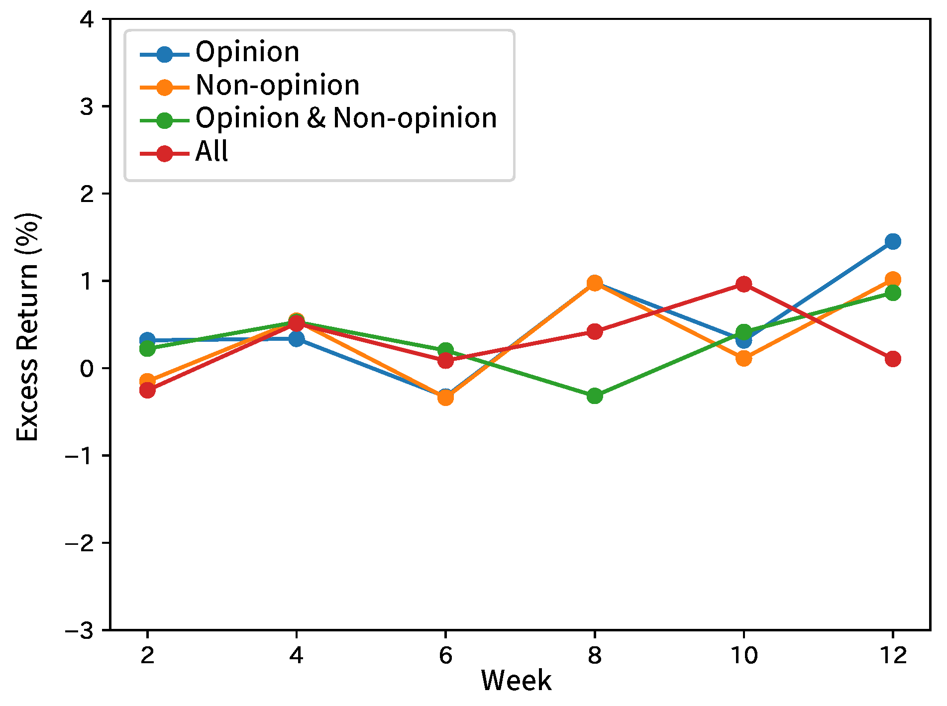
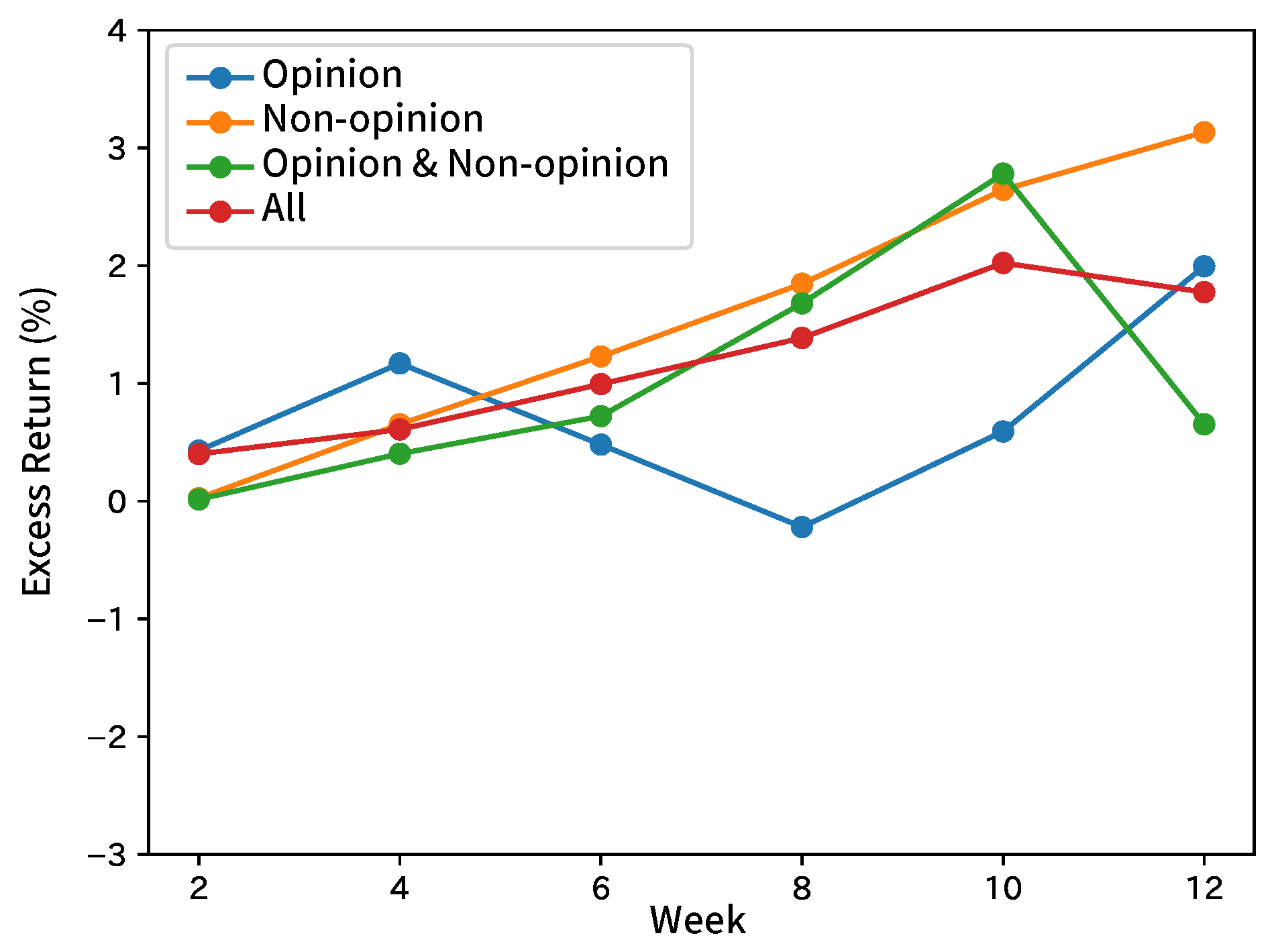
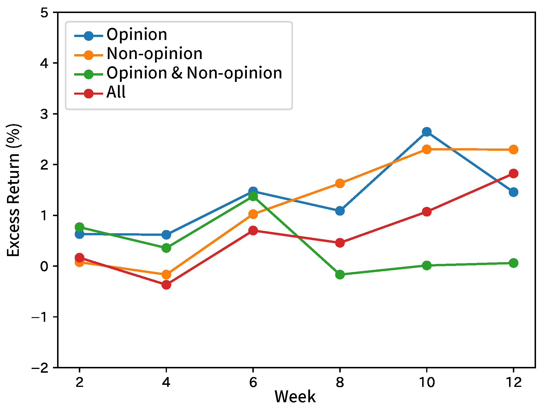
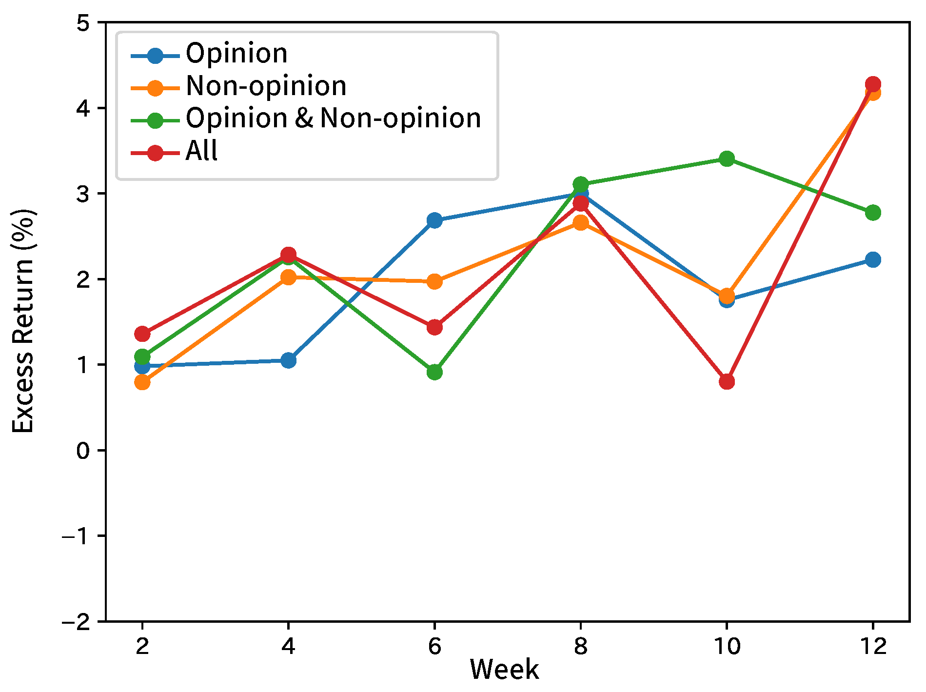
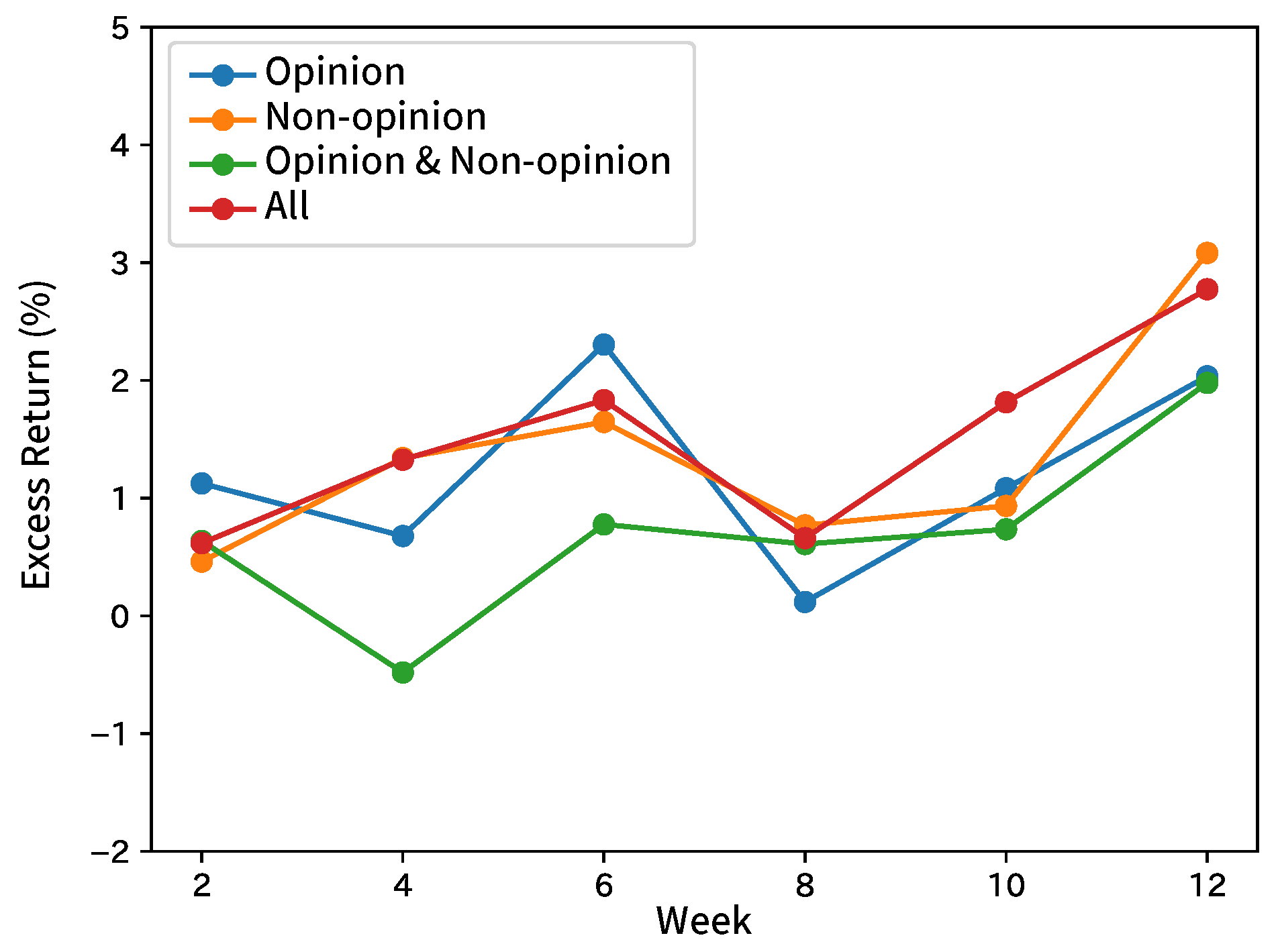
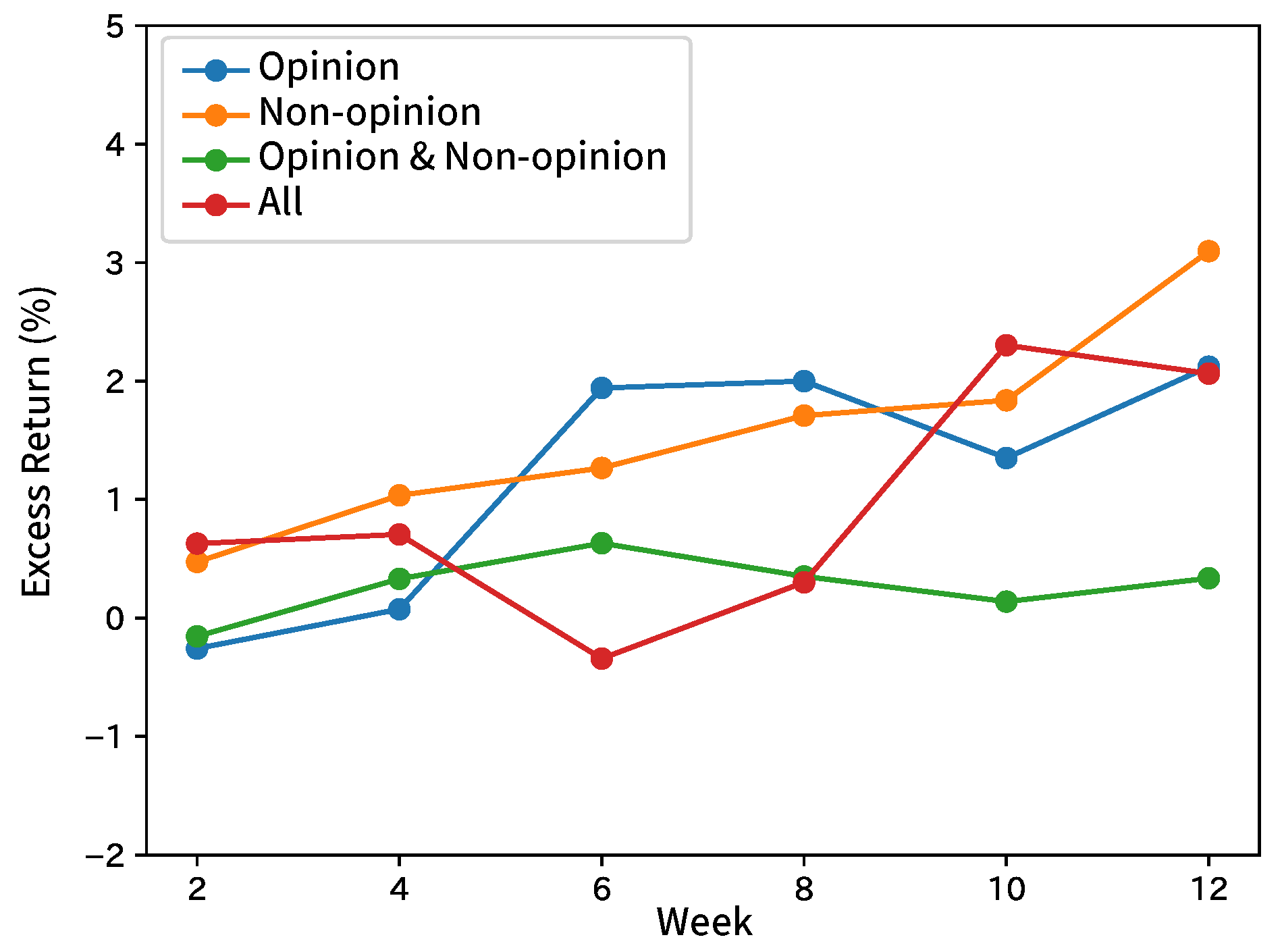
Table 4 shows the summary by taking the average of the results by broker and input sentence. Table 5 shows the summary of each index and the results of the comparison methods. Figure 4, Figure 5, Figure 6, Figure 7 and Figure 8 show the time-series excess returns of long/short strategies with the results obtained by the brokers.
7.2. Forecasting Movements of Stock Prices
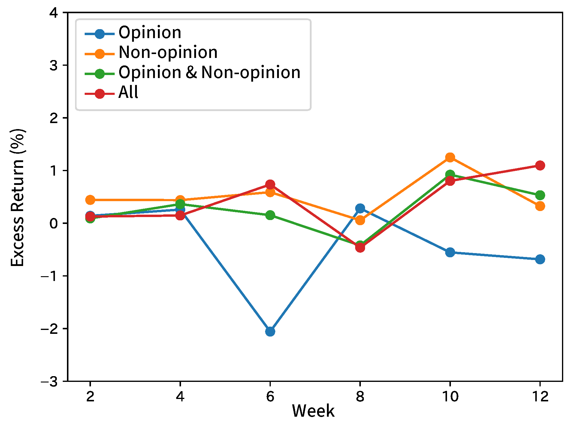
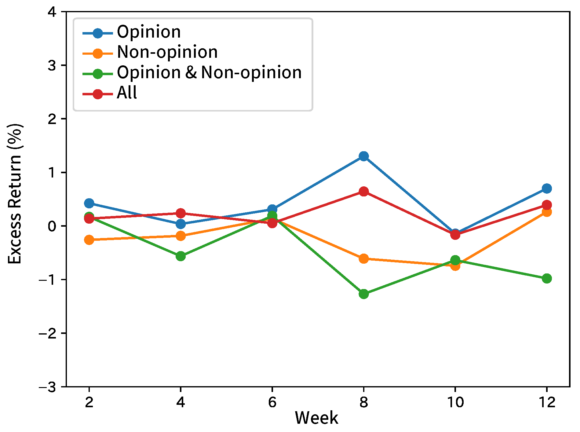
Table 6 and Table 7 show the summary by taking the average of the results by broker and input sentence. Table 8 and Table 9 show the summaries with the results of the comparison methods. Figure 9, Figure 10, Figure 11, Figure 12 and Figure 13 show the graphs of gained excess returns of long/short strategies with results obtained by the brokers. Table 10 shows the results of the multitask.
8. Discussion
8.1. Forecasting Movements of Analyst Net Income Estimates
In Table 4, for Brokers A, D, and E, F1 was the highest when inputting only non-opinion sentences. For Broker B, F1 was the highest when inputting opinion and non-opinion sentences separately. For Broker C, F1 was the highest when inputting only opinion sentences. Analysts in Broker C revise their estimated incomes based on their long-term views expressed as opinion sentences in the context of reports, while analysts in Broker A, D, and E put more weights on facts mainly released from target companies to revise their estimated incomes. This would make a difference. The basis of the forecast would differ for each broker. In this experiment, the distinction between opinion and non-opinion sentences were effective in forecasting. A high F1 of about 0.90 was obtained when inputting non-opinion sentences or all sentences of Broker D, but no result of Brokers A and E reached F1 of 0.70. Therefore, these are considered as brokers that are easy to analyze. When compared to the comparison methods, the most results of our method were clearly better than those of RF and RNN without inputting the trend in terms of p-values. In addition, our method performs slightly better than SVM. As the accuracy was higher than that of the RNN without inputting the trend, it is more effective to add the trend. Besides, SVM inputting only sentences in analyst reports also obtained such a high F1 that contexts of analyst reports were also effective for the forecast. Further improvement in the F1 score can be obtained by analyzing both analyst reports and the trend. For instance, constructing hierarchical attentions [31], instead of insertion from a hidden layer of MLP, would check how effective the trend and analyst reports are. The returns with the long/short strategy were more positive than negative, but the graphs were not monotone.
In the results of Broker D, the inputs of non-opinion sentences with high F1 scores increase monotonically in return, but those of all sentences with relatively high F1 scores fall below 0 in the 6th week. This indicates a low correlation of F1 scores and returns, which is attributed to the stock market being affected by the performance of each stock, as well as political and other economic conditions. The reason may be that the movement of a stock price is affected not only by the direction of net income estimate but also by other factors such as political and economic conditions.
8.2. Forecasting Movements of Stock Prices
The average F1 score of the excess return was 0.52 and that of the volatility was 0.60. There were no significant differences among the three input methods, such as inputting only opinion sentences, inputting only non-opinion sentences, and inputting opinion and non-opinion sentences separately. The difference between opinion and non-opinion sentences was ineffective in forecasting stock price movements. However, the best ways of the inputs were different by broker. We could not find advantages with our method over the comparison methods in terms of p-values. Therefore, the superiority of our method in this experiment was not found. As illustrated in Section 8.1, excess returns and volatilities contain random elements as well as stock prices, so it is difficult for humans to forecast. Therefore, there is no accurate forecasting in any method. The returns (Figure 9, Figure 10, Figure 11, Figure 12 and Figure 13) did not show any features, such as monotone increasing in the whole.
In the multitask experiment, the F1 score did not considerably exceed 0.5, which was expected under a random condition. The experiment was not performed well because the issuing brokers did not have a significant effect on forecasting stock price movements. In addition, forecasting stock price movements was a difficult task. It is thought to have been made more complex by learning issuing brokers.
9. Conclusions
This study aimed at obtaining unique information from the analyst reports. We propose a method to forecast analyst’s net income estimates and movements of stock prices from opinion and non-opinion sentences extracted from analyst reports with the combination of RNNs, an attention mechanism, and MLP. Under the assumption that opinion sentences of analysts are effective in forecasting analysts’ net income estimates and stock price movements, we distinguished opinion and non-opinion sentences from analyst reports. We performed the distinction with the F1 score exceeding 0.8. In this pre-experiment, word embeddings derived from the corpus of analyst reports achieved the best performance.
Next, using opinion and non-opinion sentences extracted from analyst reports, as well as analyst’s estimate trends, we forecasted that analyst’s net income estimate was higher or lower than the threshold. By broker, various inputs that had a high F1 score existed, such as the input of only opinion sentences, that of only non-opinion sentences, and that of opinion and non-opinion sentences separately. This difference results from the difference of an analyst’s net income estimate based on his/her opinions or based on facts. The basis of estimates is thought to be different by broker. In forecasting estimated net incomes, the distinction between opinion and non-opinion sentences was effective. In addition, the division of inputs by the brokers was effective because of the difference obtained between brokers. The input of the trends, the information except for the analyst reports, was also effective because the F1 score of our method was higher than that of the method without inputting the trend. We also calculated the returns under the condition of long/short strategies. However, the correlation with F1 was low.
Finally, we forecasted the movements of stock prices with opinion and non-opinion sentences in analyst reports. In this experiment, we used the excess returns and volatilities as targets. F1 scores were around 0.5 and 0.6 in the experiments of excess returns and volatilities, respectively. The forecasting accuracy did not increase. The reason for this is attributed to the difficulty which we could not forecast only by current situation analysis gained from analyst reports. Furthermore, we performed multitask learning, which learned brokers and positive/negative excess returns simultaneously. However, the F1 score was around 0.5 and we could not obtain higher accuracy. In forecasting stock price movements, the distinction between opinion and non-opinion sentences was not effective. In this research, we mainly focused on opinion sentences and non-opinion sentences. Besides these sentences, we gained results of the other indices, such as a week and a broker. We can investigate the relationships between the results of these indices.
We forecasted with analyst reports and the trend in this study. However, we can add other indices not only from the hidden layer of MLP but also from another point. Analyst reports are expected to have different bases depending on the analyst who wrote them, rather than the issuing broker. Then, the experiments conducted by analysts assist in comparing the results obtained by them. Besides, the performance can be improved by constructing the network and adding the information of analysts. The effect of analyst reports on stock prices is different in terms of analyst’s popularity. Therefore, adding the analyst’s information may make it possible to consider the difference by the analyst’s popularity and the difference in the point where an analyst emphasized as of the ground.
Author Contributions
Data curation, Y.I.; Formal analysis, M.S.; Investigation, M.S.; Methodology, H.S.; Project administration, H.S. and K.I.; Resources, H.M.; Software, M.S. and H.S.; Supervision, H.S. and K.I.; Writing—original draft, M.S.; Writing—review & editing, H.S. and Y.I. All authors have read and agreed to the published version of the manuscript.
Funding
This research received no external funding.
Acknowledgments
The authors thank S. Ikeda and T. Morita for useful discussions. We also thank K. Kasaoka for sharing the dataset with us.
Conflicts of Interest
The authors declare no conflict of interest.
References
- Bollen, J.; Mao, H.; Zeng, X. Twitter mood predicts the stock market. J. Comput. Sci. 2011, 2, 1–8. [Google Scholar] [CrossRef] [Green Version]
- Khadjeh Nassirtoussi, A.; Aghabozorgi, S.; Ying Wah, T.; Ngo, D.C.L. Text mining for market prediction: A systematic review. Expert Syst. Appl. 2014, 41, 7653–7670. [Google Scholar] [CrossRef]
- Schumaker, R.P.; Chen, H. Textual Analysis of Stock Market Prediction Using Breaking Financial News: The AZFin Text System. ACM Trans. Inf. Syst. 2009, 27, 1–19. [Google Scholar] [CrossRef]
- Schumaker, R.P.; Zhang, Y.; Huang, C.N.; Chen, H. Evaluating sentiment in financial news articles. Decis. Support Syst. 2012, 53, 458–464. [Google Scholar] [CrossRef]
- Koppel, M.; Shtrimberg, I. Good News or Bad News? Let the Market Decide. In Computing Attitude and Affect in Text: Theory and Applications; Shanahan, J.G., Qu, Y., Wiebe, J., Eds.; Springer: Dordrecht, The Netherland, 2006; pp. 297–301. [Google Scholar]
- Low, B.T.; Chan, K.; Choi, L.L.; Chin, M.Y.; Lay, S.L. Semantic expectation-based causation knowledge extraction: A study on Hong Kong stock movement analysis. In Proceedings of the Pacific-Asia Conference on Knowledge Discovery and Data Mining (PAKDD), Hong Kong, China, 16–18 April 2001; pp. 114–123. [Google Scholar]
- Ito, T.; Sakaji, H.; Tsubouchi, K.; Izumi, K.; Yamashita, T. Text-visualizing Neural Network Model: Understanding Online Financial Textual Data. In Proceedings of the Pacific-Asia Conference on Knowledge Discovery and Data Mining (PAKDD), Melbourne, Australia, 3–6 June 2018; pp. 247–259. [Google Scholar]
- Ito, T.; Sakaji, H.; Izumi, K.; Tsubouchi, K.; Yamashita, T. GINN: Gradient interpretable neural networks for visualizing financial texts. Int. J. Data Sci. Anal. 2020, 9, 431–445. [Google Scholar] [CrossRef]
- Milea, V.; Sharef, N.M.; Almeida, R.J.; Kaymak, U.; Frasincar, F. Prediction of the MSCI EURO index based on fuzzy grammar fragments extracted from European Central Bank statements. In Proceedings of the 2010 International Conference of Soft Computing and Pattern Recognition, Paris, France, 7–10 December 2010; pp. 231–236. [Google Scholar] [CrossRef] [Green Version]
- Wuthrich, B.; Cho, V.; Leung, S.; Permunetilleke, D.; Sankaran, K.; Zhang, J. Daily stock market forecast from textual web data. In Proceedings of the SMC’98 Conference Proceedings, 1998 IEEE International Conference on Systems, Man, and Cybernetics (Cat. No.98CH36218), San Diego, CA, USA, 14 October 1998; Volume 3, pp. 2720–2725. [Google Scholar]
- Bar-Haim, R.; Dinur, E.; Feldman, R.; Fresko, M.; Goldstein, G. Identifying and Following Expert Investors in Stock Microblogs. In Proceedings of the 2011 Conference on Empirical Methods in Natural Language Processing, Scotland, UK, 27–31 July 2011; Association for Computational Linguistics: Stroudsburg, PA, USA, 2011; pp. 1310–1319. [Google Scholar]
- Guijarro, F.; Moya-Clemente, I.; Saleemi, J. Liquidity Risk and Investors’ Mood: Linking the Financial Market Liquidity to Sentiment Analysis through Twitter in the S&P500 Index. Sustainability 2019, 11, 7048. [Google Scholar] [CrossRef] [Green Version]
- Vu, T.T.; Chang, S.; Ha, Q.T.; Collier, N. An Experiment in Integrating Sentiment Features for Tech Stock Prediction in Twitter. In Proceedings of the Workshop on Information Extraction and Entity Analytics on Social Media Data, Mumbai, India, 9 December 2012; The COLING 2012 Organizing Committee: Mumbai, India, 2012; pp. 23–38. [Google Scholar]
- Oliveira, N.; Cortez, P.; Areal, N. The impact of microblogging data for stock market prediction: Using Twitter to predict returns, volatility, trading volume and survey sentiment indices. Expert Syst. Appl. 2017, 73, 125–144. [Google Scholar] [CrossRef] [Green Version]
- Zhang, L.; Xiao, K.; Zhu, H.; Liu, C.; Yang, J.; Jin, B. CADEN: A Context-Aware Deep Embedding Network for Financial Opinions Mining. In Proceedings of the 2018 IEEE International Conference on Data Mining (ICDM), Singapore, 17–20 November 2018; pp. 757–766. [Google Scholar]
- Ranco, G.; Aleksovski, D.; Caldarelli, G.; Grčar, M.; Mozetič, I. The Effects of Twitter Sentiment on Stock Price Returns. PLoS ONE 2015, 10, e0138441. [Google Scholar] [CrossRef] [PubMed] [Green Version]
- Smailović, J.; Grčar, M.; Lavrač, N.; Žnidaršič, M. Predictive Sentiment Analysis of Tweets: A Stock Market Application. In Human-Computer Interaction and Knowledge Discovery in Complex, Unstructured, Big Data; Holzinger, A., Pasi, G., Eds.; Springer: Berlin/Heidelberg, Germany, 2013; pp. 77–88. [Google Scholar]
- Sakaji, H.; Sakai, H.; Masuyama, S. Automatic Extraction of Basis Expressions That Indicate Economic Trends. In Proceedings of the Pacific-Asia Conference on Knowledge Discovery and Data Mining (PAKDD), Osaka, Japan, 20–23 May 2008; pp. 977–984. [Google Scholar]
- Sakaji, H.; Murono, R.; Sakai, H.; Bennett, J.; Izumi, K. Discovery of Rare Causal Knowledge from Financial Statement Summaries. In Proceedings of the 2017 IEEE Symposium on Computational Intelligence for Financial Engineering and Economics (CIFEr), Kolkata, India, 24–25 March 2017; pp. 602–608. [Google Scholar]
- Kitamori, S.; Sakai, H.; Sakaji, H. Extraction of sentences concerning business performance forecast and economic forecast from summaries of financial statements by deep learning. In Proceedings of the 2017 IEEE Symposium Series on Computational Intelligence (SSCI), Honolulu, HI, USA, 27 November–1 December 2017; pp. 1–7. [Google Scholar]
- Hirano, M.; Sakaji, H.; Kimura, S.; Izumi, K.; Matsushima, H.; Nagao, S.; Kato, A. Selection of Related Stocks using Financial Text Mining. In Proceedings of the 2018 IEEE International Conference on Data Mining Workshops (ICDMW), Singapore, 17–20 November 2018; pp. 191–198. [Google Scholar]
- Hirano, M.; Sakaji, H.; Kimura, S.; Izumi, K.; Matsushima, H.; Nagao, S.; Kato, A. Related Stocks Selection with Data Collaboration Using Text Mining. Information 2019, 10, 102. [Google Scholar] [CrossRef] [Green Version]
- Mikolov, T.; Chen, K.; Corrado, G.; Dean, J. Efficient Estimation of Word Representations in Vector Space. arXiv 2013, arXiv:1301.3781. [Google Scholar]
- Sato, T. Neologism Dictionary Based on the Language Resources on the WEB for Mecab. 2015. Available online: https://github.com/neologd/mecab-ipadic-neologd (accessed on 28 April 2020).
- Sato, T.; Hashimoto, T.; Okumura, M. Operation of a word segmentation dictionary generation system called NEologd. In Proceedings of the Information Processing Society of Japan, Special Interest Group on Natural Language Processing (IPSJ-SIGNL), Tokyo, Japan, 20–22 December 2016; p. NL-229-15. [Google Scholar]
- Sato, T.; Hashimoto, T.; Okumura, M. Implementation of a word segmentation dictionary called mecab-ipadic-NEologd and study on how to use it effectively for information retrieval. In Proceedings of the Twenty-three Annual Meeting of the Association for Natural Language Processing, Tsukuba, Japan, 14–16 March 2017. [Google Scholar]
- Jeffrey, P.; Richard, S.; Christopher, M. GloVe: Global Vectors for Word Representation. In Proceedings of the 2014 Conference on Empirical Methods in Natural Language Processing (EMNLP 2014), Association for Computational Linguistics, Doha, Qatar, 25–29 October 2014; pp. 1532–1543. [Google Scholar]
- Hochreiter, S.; Schmidhuber, J. Long short-term memory. Neural Comput. 1997, 9, 1735–1780. [Google Scholar] [CrossRef] [PubMed]
- Graves, A.; Schmidhuber, J. Framewise phoneme classification with bidirectional LSTM and other neural network architectures. Neural Netw. 2005, 18, 602–610. [Google Scholar] [CrossRef] [PubMed]
- Cho, K.; van Merriënboer, B.; Gulcehre, C.; Bahdanau, D.; Bougares, F.; Schwenk, H.; Bengio, Y. Learning Phrase Representations using RNN Encoder–Decoder for Statistical Machine Translation. In Proceedings of the 2014 Conference on Empirical Methods in Natural Language Processing (EMNLP), Association for Computational Linguistics, Doha, Qatar, 25–29 October 2014; pp. 1724–1734. [Google Scholar]
- Yang, Z.; Yang, D.; Dyer, C.; He, X.; Smola, A.; Hovy, E. Hierarchical Attention Networks for Document Classification. In Proceedings of the 2016 Conference of the North American Chapter of the Association for Computational Linguistics: Human Language Technologies, Association for Computational Linguistics, San Diego, CA, USA, 12–17 June 2016; pp. 1480–1489. [Google Scholar] [CrossRef] [Green Version]
Figure 1.
Flow of experiments in this paper. This paper focuses on three experiments: opinion sentence extract, net income estimate forecast, and stock price forecast. The opinion sentence extraction is conducted as a pre-experiment.
Figure 1.
Flow of experiments in this paper. This paper focuses on three experiments: opinion sentence extract, net income estimate forecast, and stock price forecast. The opinion sentence extraction is conducted as a pre-experiment.

Figure 2.
Overview of our method. Sentences are split into words using MeCab. Words are converted to word embeddings using GloVe. We input these word embeddings to bidirectional LSTM or GRU. The outputs of the hidden layers are weighted by the attention mechanism. We input the weighted output to MLP and softmax function. Then, the probability of each label is output.

Figure 3.
Overview of our method with inputs of opinion and non-opinion sentences. From the word embedding to the attention, opinion and non-opinion sentences go through separately. Then, the weighted outputs of RNNs are concatenated and input to MLP.
Figure 3.
Overview of our method with inputs of opinion and non-opinion sentences. From the word embedding to the attention, opinion and non-opinion sentences go through separately. Then, the weighted outputs of RNNs are concatenated and input to MLP.

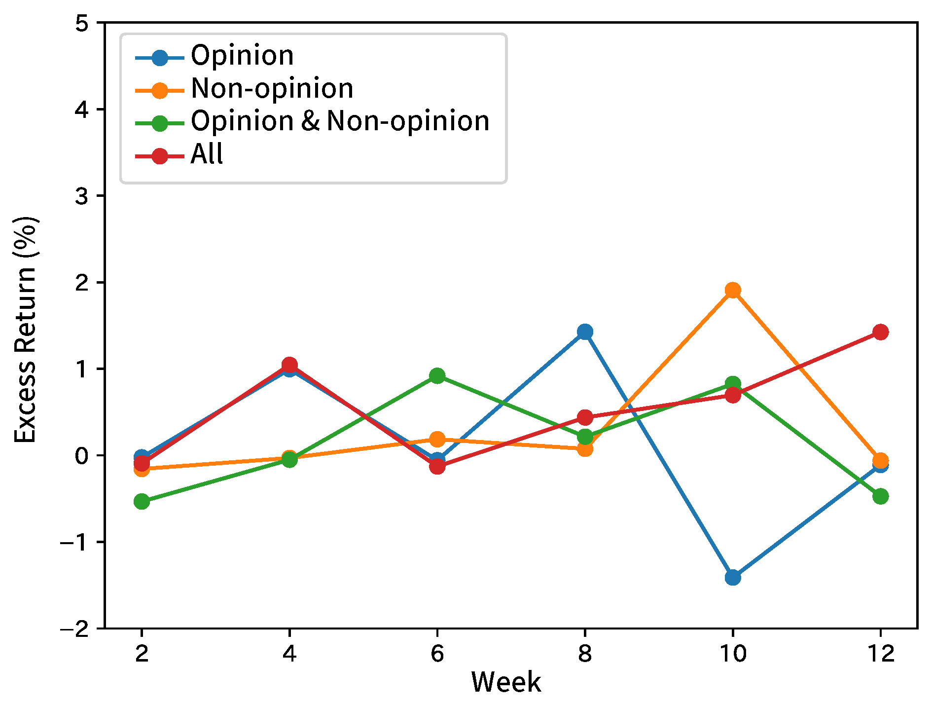
Figure 4.
Excess returns of Broker A in forecasting analyst net income estimates.

Figure 5.
Excess returns of Broker B in forecasting analyst net income estimates.

Figure 6.
Excess returns of Broker C in forecasting analyst net income estimates.

Figure 7.
Excess returns of Broker D in forecasting analyst net income estimates.

Figure 8.
Excess returns of Broker E in forecasting analyst net income estimates.

Figure 9.
Excess returns of Broker A in forecasting excess returns.

Figure 10.
Excess returns of Broker B in forecasting excess returns.

Figure 11.
Excess returns of Broker C in forecasting excess returns.

Figure 12.
Excess returns of Broker D in forecasting excess returns.

Figure 13.
Excess returns of Broker E in forecasting excess returns.


Table 1.
Number of reports of positive or negative excess returns.
| Period | Positive Excess Returns | Negative Excess Returns |
|---|---|---|
| 2 weeks | 8516 | 8840 |
| 4 weeks | 8620 | 8736 |
| 6 weeks | 8804 | 8552 |
| 8 weeks | 8774 | 8582 |
| 10 weeks | 8814 | 8542 |
| 12 weeks | 8686 | 8670 |
Table 2.
Typical examples of opinion and non-opinion sentences in analyst reports. English follows Japanese.
Table 2.
Typical examples of opinion and non-opinion sentences in analyst reports. English follows Japanese.
| Opinion/Non-Opinion | Sentence |
|---|---|
| Opinion |  (We will revise our earnings forecast downwards based on 2Q results.) |
| Opinion |  (The factors that could reduce profitability are the launch of new production bases and R&D investment.) |
| Non-opinion |  (This term sales reached a record high of 10 billion yen.) |
| Non-opinion |  (The dividend is planned to be 270 yen for the interim period of September 2007, 120 yen and 150 yen at the end of the year.) |
Table 3.
Results of opinion sentence extraction (pre-experiment). The evaluation index is Macro-F1. SVM and RF do not use word embeddings, so the corpus is indicated by a hyphen (-).
Table 3.
Results of opinion sentence extraction (pre-experiment). The evaluation index is Macro-F1. SVM and RF do not use word embeddings, so the corpus is indicated by a hyphen (-).
| Model | Corpus | F1 |
|---|---|---|
| Our Method | Analyst Report Sentences | 0.835 |
| Our Method | Analyst Report Set | 0.836 |
| Our Method | Reuters | 0.820 |
| Our Method | Wikipedia | 0.809 |
| Our Method | Nikkei News | 0.822 |
| SVM | - | 0.780 |
| RF | - | 0.664 |
Table 4.
Summary by broker in forecasting analyst net income estimates with our method. Macro-F1 is a measure.
Table 4.
Summary by broker in forecasting analyst net income estimates with our method. Macro-F1 is a measure.
| Broker | Opinion Sentences | Non-Opinion Sentences | Opinion and Non-Opinion Sentences | All Sentences |
|---|---|---|---|---|
| A | 0.643 | 0.653 | 0.612 | 0.543 |
| B | 0.701 | 0.680 | 0.777 | 0.703 |
| C | 0.776 | 0.687 | 0.666 | 0.725 |
| D | 0.587 | 0.907 | 0.548 | 0.904 |
| E | 0.631 | 0.695 | 0.664 | 0.594 |
Table 5.
Summary of forecasting movements of analyst net income estimates. Macro-F1 is a measure. The scores of SVM and RF in the row of input: opinion and non-opinion sentences are indicated by hyphens (-) because SVM and RF cannot have inputs of opinion and non-opinion sentences separately.
Table 5.
Summary of forecasting movements of analyst net income estimates. Macro-F1 is a measure. The scores of SVM and RF in the row of input: opinion and non-opinion sentences are indicated by hyphens (-) because SVM and RF cannot have inputs of opinion and non-opinion sentences separately.
| Index | Our Method | RNN without the Trend | SVM | RF |
|---|---|---|---|---|
| Input: opinion sentences | 0.668 | 0.610 | 0.657 | 0.596 |
| Input: non-opinion sentences | 0.724 | 0.605 | 0.654 | 0.594 |
| Input: opinion and non-opinion sentences | 0.653 | 0.611 | - | - |
| Input: all sentences | 0.694 | 0.627 | 0.691 | 0.624 |
| Broker: A | 0.613 | 0.615 | 0.642 | 0.596 |
| Broker: B | 0.715 | 0.658 | 0.746 | 0.574 |
| Broker: C | 0.713 | 0.617 | 0.678 | 0.649 |
| Broker: D | 0.736 | 0.604 | 0.653 | 0.637 |
| Broker: E | 0.646 | 0.573 | 0.620 | 0.568 |
| Period: 2 weeks | 0.710 | 0.614 | 0.668 | 0.602 |
| Period: 4 weeks | 0.674 | 0.614 | 0.666 | 0.601 |
| Period: 6 weeks | 0.679 | 0.606 | 0.668 | 0.608 |
| Period: 8 weeks | 0.683 | 0.611 | 0.671 | 0.610 |
| Period: 10 weeks | 0.686 | 0.616 | 0.666 | 0.603 |
| Period: 12 weeks | 0.678 | 0.618 | 0.667 | 0.604 |
significant at 5% compared to our method; significant at 1% compared to our method.
Table 6.
Summary by broker in forecasting excess returns with our method. Macro-F1 is a measure.
| Broker | Opinion Sentences | Non-Opinion Sentences | Opinion and Non-Opinion Sentences | All Sentences |
|---|---|---|---|---|
| A | 0.529 | 0.526 | 0.520 | 0.506 |
| B | 0.558 | 0.563 | 0.569 | 0.573 |
| C | 0.530 | 0.535 | 0.503 | 0.533 |
| D | 0.518 | 0.525 | 0.509 | 0.523 |
| E | 0.500 | 0.503 | 0.492 | 0.499 |
Table 7.
Summary by broker in forecasting volatiles with our method. Macro-F1 is a measure.
| Broker | Opinion Sentences | Non-Opinion Sentences | Opinion and Non-Opinion Sentences | All Sentences |
|---|---|---|---|---|
| A | 0.618 | 0.587 | 0.630 | 0.596 |
| B | 0.634 | 0.633 | 0.657 | 0.657 |
| C | 0.585 | 0.626 | 0.593 | 0.638 |
| D | 0.575 | 0.581 | 0.575 | 0.588 |
| E | 0.568 | 0.584 | 0.590 | 0.601 |
Table 8.
Summary of forecasting excess returns. Macro-F1 is a measure. The scores of SVM and RF in the row of input: opinion and non-opinion sentences are indicated by hyphens (-) because SVM and RF cannot have separates inputs for opinion and non-opinion sentences.
Table 8.
Summary of forecasting excess returns. Macro-F1 is a measure. The scores of SVM and RF in the row of input: opinion and non-opinion sentences are indicated by hyphens (-) because SVM and RF cannot have separates inputs for opinion and non-opinion sentences.
| Index | Our Method | SVM | RF |
|---|---|---|---|
| Input: opinion sentences | 0.527 | 0.549 | 0.499 |
| Input: non-opinion sentences | 0.530 | 0.546 | 0.484 |
| Input: opinion and non-opinion sentences | 0.519 | - | - |
| Input: all sentences | 0.527 | 0.556 | 0.509 |
| Broker: A | 0.520 | 0.527 | 0.484 |
| Broker: B | 0.566 | 0.619 | 0.508 |
| Broker: C | 0.525 | 0.542 | 0.520 |
| Broker: D | 0.519 | 0.546 | 0.516 |
| Broker: E | 0.499 | 0.518 | 0.489 |
| Period: 2 weeks | 0.519 | 0.537 | 0.473 |
| Period: 4 weeks | 0.519 | 0.542 | 0.494 |
| Period: 6 weeks | 0.523 | 0.546 | 0.494 |
| Period: 8 weeks | 0.525 | 0.546 | 0.505 |
| Period: 10 weeks | 0.525 | 0.564 | 0.522 |
| Period: 12 weeks | 0.532 | 0.569 | 0.532 |
significant at 5% compared to our method; significant at 1% compared to our method.
Table 9.
Summary of forecasting volatilities. Macro-F1 is a measure. The scores of SVM and RF in the row of input: opinion and non-opinion sentences are indicated by hyphens (-) because SVM and RF cannot have separate inputs of opinion and non-opinion sentences.
Table 9.
Summary of forecasting volatilities. Macro-F1 is a measure. The scores of SVM and RF in the row of input: opinion and non-opinion sentences are indicated by hyphens (-) because SVM and RF cannot have separate inputs of opinion and non-opinion sentences.
| Index | Our Method | SVM | RF |
|---|---|---|---|
| Input: opinion sentences | 0.596 | 0.648 | 0.628 |
| Input: non-oppinion sentences | 0.602 | 0.666 | 0.633 |
| Input: opinion and non-opinion sentences | 0.609 | - | - |
| Input: all sentences | 0.616 | 0.698 | 0.659 |
| Broker: A | 0.608 | 0.669 | 0.654 |
| Broker: B | 0.646 | 0.726 | 0.662 |
| Broker: C | 0.611 | 0.665 | 0.641 |
| Broker: D | 0.580 | 0.637 | 0.608 |
| Broker: E | 0.586 | 0.657 | 0.636 |
| Period: 2 weeks | 0.562 | 0.629 | 0.607 |
| Period: 4 weeks | 0.593 | 0.655 | 0.629 |
| Period: 6 weeks | 0.618 | 0.674 | 0.646 |
| Period: 8 weeks | 0.613 | 0.680 | 0.653 |
| Period: 10 weeks | 0.616 | 0.693 | 0.657 |
| Period: 12 weeks | 0.633 | 0.693 | 0.649 |
significant at 5% compared to our method; significant at 1% compared to our method.
Table 10.
Results of the multitask. Macro-F1 is a measure.
| Period | Opinion Sentences | Non-Opinion Sentences | Opinion and Non-Opinion Sentences | All Sentences |
|---|---|---|---|---|
| 2 weeks | 0.502 | 0.510 | 0.509 | 0.497 |
| 4 weeks | 0.521 | 0.515 | 0.516 | 0.517 |
| 6 weeks | 0.502 | 0.516 | 0.539 | 0.540 |
| 8 weeks | 0.527 | 0.523 | 0.529 | 0.539 |
| 10 weeks | 0.549 | 0.510 | 0.540 | 0.552 |
| 12 weeks | 0.547 | 0.547 | 0.525 | 0.544 |
© 2020 by the authors. Licensee MDPI, Basel, Switzerland. This article is an open access article distributed under the terms and conditions of the Creative Commons Attribution (CC BY) license (http://creativecommons.org/licenses/by/4.0/).
Share and Cite
MDPI and ACS Style
Suzuki, M.; Sakaji, H.; Izumi, K.; Matsushima, H.; Ishikawa, Y. Forecasting Net Income Estimate and Stock Price Using Text Mining from Economic Reports. Information 2020, 11, 292. https://doi.org/10.3390/info11060292
AMA Style
Suzuki M, Sakaji H, Izumi K, Matsushima H, Ishikawa Y. Forecasting Net Income Estimate and Stock Price Using Text Mining from Economic Reports. Information. 2020; 11(6):292. https://doi.org/10.3390/info11060292
Chicago/Turabian StyleSuzuki, Masahiro, Hiroki Sakaji, Kiyoshi Izumi, Hiroyasu Matsushima, and Yasushi Ishikawa. 2020. "Forecasting Net Income Estimate and Stock Price Using Text Mining from Economic Reports" Information 11, no. 6: 292. https://doi.org/10.3390/info11060292
Note that from the first issue of 2016, this journal uses article numbers instead of page numbers. See further details here.