Public Traffic Congestion Estimation Using an Artificial Neural Network


1
State Key Laboratory of Information Engineering in Surveying, Mapping and Remote Sensing, Wuhan University, Wuhan 430079, China
2
Collaborative Innovation Center for Geospatial Information Technology, Wuhan 430079, China
3
Faculty of Geomatics, East China University of Technology, Nanchang 330013, China
*
Author to whom correspondence should be addressed.
ISPRS Int. J. Geo-Inf. 2020, 9(3), 152; https://doi.org/10.3390/ijgi9030152
Submission received: 20 January 2020
/
Revised: 18 February 2020
/
Accepted: 7 March 2020
/
Published: 8 March 2020
(This article belongs to the Special Issue GIS in Sustainable Transportation)
Abstract
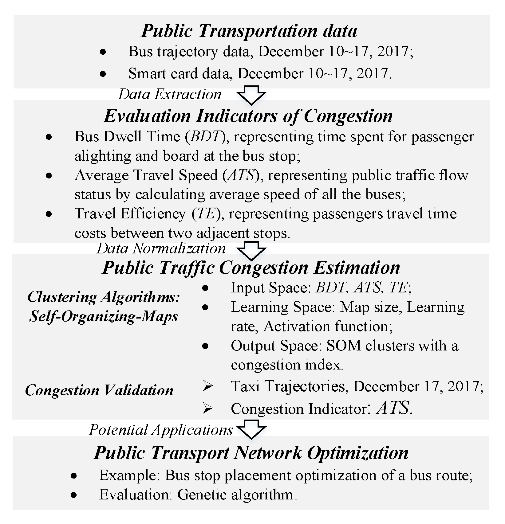
:Alleviating public traffic congestion is an efficient and effective way to improve the travel time reliability and quality of public transport services. The existing public network optimization models usually ignored the essential impact of public traffic congestion on the performance of public transport service. To address this problem, this study proposes a data-based methodology to estimate the traffic congestion of road segments between bus stops (RSBs). The proposed methodology involves two steps: (1) Extracting three traffic indicators of the RSBs from smart card data and bus trajectory data; (2) The self-organizing map (SOM) is used to cluster and effectively recognize traffic patterns embedded in the RSBs. Furthermore, a congestion index for ranking the SOM clusters is developed to determine the congested RSBs. A case study using real-world datasets from a public transport system validates the proposed methodology. Based on the congested RSBs, an exploratory example of public transport network optimization is discussed and evaluated using a genetic algorithm. The clustering results showed that the SOM could suitably reflect the traffic characteristics and estimate traffic congestion of the RSBs. The results obtained in this study are expected to demonstrate the usefulness of the proposed methodology in sustainable public transport improvements.
1. Introduction
A well-developed public transport system is the key to achieving citizens’ mobility in an environmentally sustainable fashion. Due to demand fluctuations and traffic congestion, it is a challenging task for operators to ensure the efficiency of public transport service and improve travel time reliability [1]. Unreliable service causes passengers to require extra travel time due to the headway irregularity of buses, and imposes additional costs on operators because of the ineffective utilization of allocated resources. Therefore, there is a growing realization that the alleviation of traffic congestion through public transport network (PTN) optimization is a fundamental solution to reduce high traffic congestion costs, lower energy consumption, lessen air pollution, and improve mobility [2].
Most of the previous PTN optimization models were formulated as bi-level problems whose objectives are to minimize both the operators’ and users’ costs [3]. In-vehicle travel time, stop spacing, frequency of service, capacity, and congestion related to over-crowded vehicles are usually considered as variables in network optimization problems. Examples of these models can be seen in the studies of References [4,5,6]. Due to the NP(non-deterministic polynomial)-hard nature of optimizing all the variables simultaneously, metaheuristic approaches that pursue worthy local optimal results are proposed. For example, Mesbah et al. [7] proposed a bi-level approach to optimize the transport road space priority for a road network using the parallel genetic algorithm. However, these network optimization models developed in the above-mentioned articles had been usually applied in uncongested road segments.
Public traffic condition refers to the traffic volume of the road network and its dynamic spatial-temporal distribution, which can reflect the degree of congestion [8]. Recently, the traffic congestion impacts of bus operations on a road segment or a corridor have been investigated by researchers [9,10]. These congestion effects mainly include the effects of bus stop design, bus travel time, and bus priority options such as exclusive bus lanes or priority signals for buses [9]. Understanding these congestion impacts can help operators to identify the effectiveness of transport network optimization in relieving congested areas or congested routes. For example, under congested traffic conditions, it is difficult for buses to return to the driving lane, which leads to a longer travel time after picking-up/dropping off passengers at stops [11]. Furthermore, the bus travel time variation dominated by traffic congestion often results in unreliable service, which has negative impacts on both the operators and passengers [12]. Previous studies have pointed out that well-located stops have the potential to alleviate the impact of traffic congestion [3]. Therefore, it is critical to optimize PTN by considering the impact of traffic congestion in order to achieve a high level of public transport service and improve travel time reliability.
In this study, we proposed a data-based methodology to estimate the traffic congestion of road segments between bus stops (RSBs) using a self-organizing feature map (SOM). The SOM was used to cluster and effectively recognize traffic patterns embedded in the RSBs. Furthermore, a congestion index for ranking the SOM clusters was developed to determine the congested RSBs. Based on the congested RSBs, an exploratory example of PTN optimization was discussed and evaluated using a genetic algorithm. The main contributions of this study were summarized as follows:
(1) Public traffic congestion estimation: We estimated the traffic congestion of the RSBs using SOM based on bus trajectory data and smart card data. In contrast to the traditional methods using taxi trajectory data, our methodology could be applied to estimate the congested RSBs with bus priority lanes or with limited taxi trips, which can benefit various applications including road traffic status estimation, PTN optimization, and urban transport system management.
(2) PTN optimization considering traffic congestion: Based on the congested RSBs, an exploratory example of PTN optimization was discussed and evaluated using a genetic algorithm. The empirical results contributed to the development of more efficient strategies for PTN optimization by considering public traffic congestion.
The rest of this paper is organized in the following way. The next section provides a literature review. Section 3 describes our proposed methodology, followed by a case study in Section 4. The discussion of the strategies for PTN optimization is provided in Section 5. Finally, we briefly conclude in Section 6 with limitations and future research directions. Figure 1 presents the research framework.
2. Literature Review
2.1. Traffic Congestion Estimation
Urban traffic congestion has become a critical problem that not only affects the daily lives of the inhabitants’ due to the loss of time, but also restricts the stable development of a city [13,14]. Estimating urban traffic congestion effectively is the first step to improve the travel time reliability for passengers and solve the urban traffic congestion problem [15]. Many studies have been conducted to study traffic congestion by using floating car data (FCD) from different aspects, including traffic congestion estimation, traffic congestion prediction, and traffic flow propagation [16,17,18]. For example, Yu et al. [19] proposed a novel approach by estimating the speed in each trajectory to detect congestion locations of road segments based on stay-place clustering. By treating the congestion level analysis as a regression problem, Wang et al. [20] proposed a locality constraint distance metric to characterize the congestion level. All the above-mentioned methods are mainly implemented depending on both road networks, traffic flow of vehicles, or POIs (Points of Interests). Recently, more research has used neural networks, support vector machines, heuristic algorithms, and fuzzy logic to estimate traffic congestion based on changes in traffic volume, occupancy, or speed [21,22,23]. For example, to estimate the traffic congestion using floating car data efficiently, Kong et al. [22] made a new fuzzy comprehensive evaluation method based on traffic flows, by assigning weights of multi-indexes. These studies provide many valuable insights into traffic congestion estimation, which can be used to ease congestion, increase safety, and improve the accuracy of traffic prediction.
The previous studies have achieved good performance in traffic congestion estimation, which provides practical applications in the fields of urban planning and PTN optimization [19]. In practice, no fixed definitions have been proposed for the level of traffic congestion, while the average travel speed for a road segment is the most commonly used indicator for traffic congestion estimation [15,24]. Unlike the above research, which focuses on the traffic status of one road segment using taxi trajectory data, the aim of our methodology is to estimate the traffic congestion of RSBs using bus trajectory data and smart card data. Our method can be applied to estimate the traffic condition of RSBs with bus priority lanes or with limited taxi trips, which can benefit various applications including bus traffic status estimation, PTN optimization, and urban transport system management.
2.2. Transport Network Optimization
The quality of transport service, in terms of reliability and accessibility, is influenced by both the external and internal factors of a public transport system [25]. Therefore, research has been conducted to explore the optimization problems for transport networks to improve the transport service quality and passenger satisfaction. Various solution methods have been applied to solve the optimization problems for transport networks with decision variables: bus stops, bus frequency, bus priority lane, etc.
(1) Bus stops: For a public bus route, one key factor that affects public transportation quality is the location of bus stops [3,11,26]. The majority of the previous studies typically treated bus stop spacing as a continuous variable by assuming that bus stops could be located anywhere along the transport routes. For example, Li and Bertini [27] optimized the bus stop spacing with archived bus stop-level demand (BSD) data based on minimizing the access cost and riding cost. To improve the service reliability of a bus service, Chien and Qin [28] formulated a mathematical model to optimize the bus stop location problem. Recently, Ceder et al. [26] developed a mathematical modeling approach to bus stop placement by considering uneven topography. Their results suggested a number of ways, including walking speed, access path attractiveness, and acceleration delay, that will lead to optimal bus stop placement.
(2) Bus frequency: Optimizing the frequency of a bus fleet can improve the transport service quality and adjust the fleet’s spatial distribution. For a public transport service, small changes in the frequency of bus routes will have an effect on the bus ridership and passengers’ travel efficiency. To improve the harmonization between social equity and public transport service level, Ruiz et al. [29] proposed a bus frequency optimization methodology. Based on bee colony optimization, Nikolic and Teodorovic [30] developed a swarm intelligence model for the transport network design problem (TNDP) by considering bus frequency and transport network optimization on each of the bus routes simultaneously. In spite of the high value for bus frequency optimization, Wang et al. [31] leveraged millions of bus transaction records, which can generate passengers’ boarding and alighting information, to infer the time-dependent traffic and customer demand.
(3) Bus priority lane: In recent years, many cities have constructed exclusive bus lanes and adopted a transport priority policy to alleviate urban traffic congestion. In terms of evaluating the impact of bus priority lane on traffic congestion, several research projects have been undertaken. Agrawal et al. [9] examined different strategies that were applied to manage shared-use bus priority lanes in the major congested urban centers of seven cities throughout the world. Based on the application of bi-level programming on bus lane planning and optimization, Yu et al. [32] proposed a bi-level model that performed well with regard to the objective of balancing the transport service level among all the bus lines. Inspired by the Braess Paradox, Bagloee et al. [33] sought congested roads by defining a merit index based on transport ridership and developed an efficient solution algorithm for searching the subset roads for the transport priority lanes.
In summary, it is revealed that traffic congestion could result in additional travel time, which would affect the service reliability of urban public transport [10,34]. However, the PTN optimization models developed in previous studies usually had been applied in the uncongested road segments, ignoring the essential impact of public traffic congestion on the performance of public transport service. Moreover, under congestion conditions, implementing the optimal models by overlooking the influence of stochastic vehicle arrivals could lead to unrealistic results. In this study, we propose a data-based methodology to estimate the traffic congestion levels of RSBs. Based on the congested RSBs, an example of PTN optimization are discussed and evaluated by using the genetic algorithm method, which contributes to the development of more efficient strategies for PTN optimization by considering public traffic congestion.
3. Methodology
In this section, we describe the proposed methodology in detail and give the definitions for the entire paper to avoid possible confusion. A comprehensive analysis of PTN requires the consideration of multiple travel times, including the passengers’ boarding/alighting time and bus dwell time at bus stops. Therefore, this study exploits several important properties about the traffic condition of the RSBs and builds a reliability-based methodology to estimate public traffic congestion.
3.1. Definitions
To make a clear statement of the bus routes and their characteristics, we will clarify some basic definitions, including the bus line, bus trajectory data, bus dwell time, average travel speed, and travel efficiency.
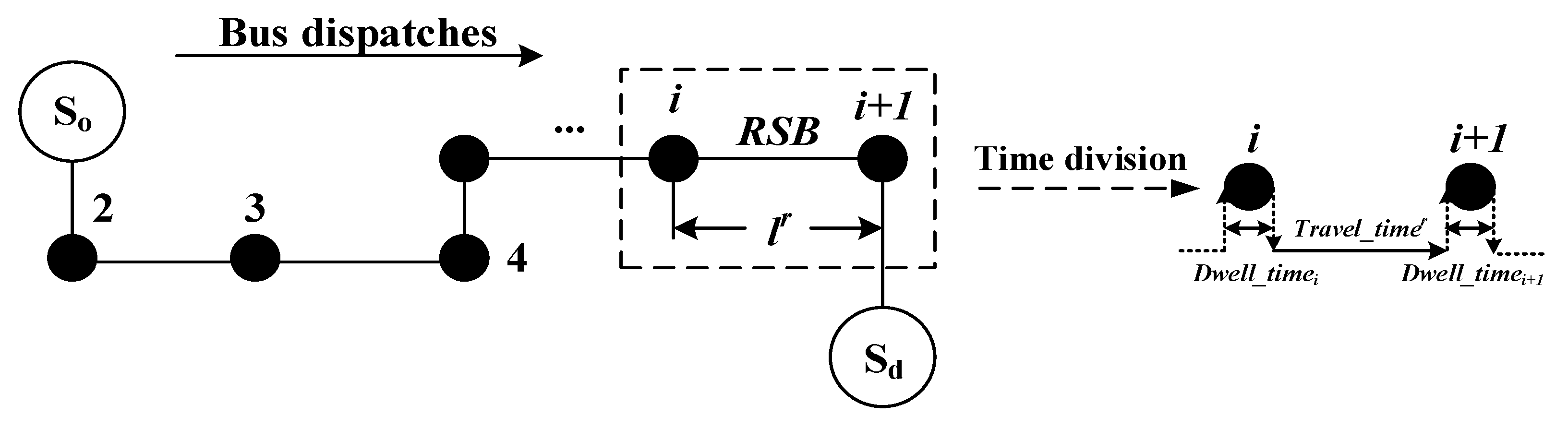
Definition 1.
Bus Line:we consider a general bus line of length L that consists of n bus stops, which is shown in Figure 2.
where
- So, Sd – Terminal bus stops of a bus line.
- RSB – One road segment between adjacent bus stops of a bus line.
- i – The index of the bus stops.
- – Length of RSB r.
Definition 2.
Bus Trajectory Data:Bus trajectory data is a dataset that describes bus movements, including the location points in a time sequence: idi, xi, yi, ti, spei, diri, while 1≤i<k, idi is a unique code for a bus, ti is a time-stamp, (xi, yi) are the latitude and longitude coordinates, spei is the bus speed and diri is the moving direction.
Definition 3.
Bus Dwell Time (BDT):Bus dwell time at bus stop i is defined as the time spent for passenger alighting and boarding. The bus dwell time is of great significance to estimate the capacity of a bus station and has also been found to depend on how congested the platform is at the bus stops [35]. The bus dwell time and travel time between adjacent bus stops i and i+1 were estimated by using the method in Reference [36].
Definition 4.
Average Travel Speed (ATS):The average travel speed describes the traffic flow status based on the average speed of each bus in an RSB, which can be calculated using the bus trajectory data. The ATS of RSB r in time interval t can be calculated as follows:
where spen is the average travel speed of each bus in RSB r in time interval t, and n is the number of buses.
Definition 5.
Travel Efficiency (TE):Travel efficiency is used to represent passengers’ travel time costs of the RSBs (the time spent of passengers travel from one bus stop to the adjacent stop). The calculation of TE r of RSB r in time interval t is shown as follows:
3.2. Congestion Estimation using an Artificial Neural Network
Public traffic congestion usually resulted in slower bus speed and longer travel time. In this study, the three main indicators used to describe the traffic congestion level of the RSBs are BDT, ATS, and TE.
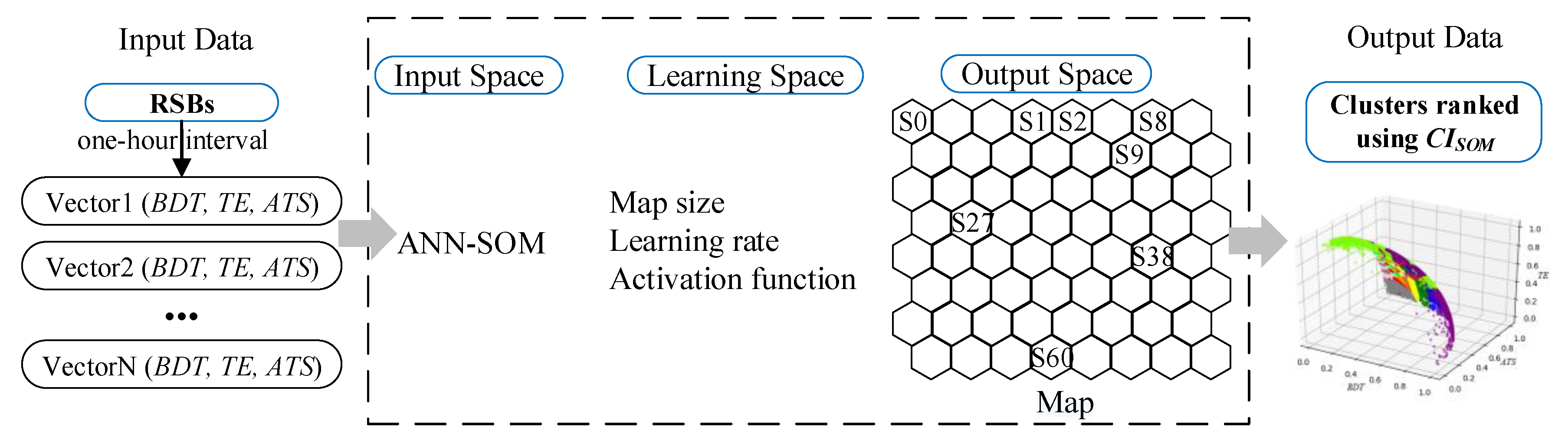
The self-organizing map (SOM) is a type of unsupervised artificial neural network model for the analysis of high-dimensional patterns in data mining applications proposed by Kohonen [37]. Based on their nearness or similarity, the SOM can classify the objects of the system into clusters, for example categories or regions [38]. Compared to traditional clustering algorithms, the SOM has three main advantages: 1) prior knowledge is not required; 2) nonlinearity can be handled; and 3) excellent visualization is provided [39]. The neurons of the SOM are distributed into two layers: the input layer and the output layer by going through a training phase. In this study, the SOM algorithm is employed to classify the RSBs based on the three traffic indicators, and the Python code is used to complete SOM learning. The flowchart of the SOM used in this study is presented in Figure 3.
In this study, each RSB comprising three traffic indicators at one-hour interval were sampled simultaneously. All input vectors (three variables: BDT, ATS, and TE) were normalized on a scale from 0 to 1. Example vectors of one RSB are shown in Table 1.
- (1)
- Initialization: Choose random values for the initial weights wi, and normalize the input vectors and weights.where x = [x1,…,xm]∈Rm represents an input vector, ||.|| represents the Euclidean norm, and M is the number of neurons.
- (2)
- Winner Finding: Find the winner neuron n, using the minimum Euclidean distance between vector x’ and weights w i’, according to Equation (5):
- (3)
- Update Weights: Adjust the weights of the winner and its neighbors at time t+1, and renormalize the weights after learning:where represents the topological neighborhood function of the winner neuron n at time t, is a positive constant called the ‘‘learning-rate’’, ri and rj are the location vectors of nodes i and j, respectively. represents the width of the kernel. The weights are updated at each time step.
- (4)
- Algorithm stop condition: Both and will decay over time. The algorithm will stop when or the prespecified number of epochs is reached.
The SOM algorithm provides effective results, which are easily visualized and interpreted from the generated maps [41]. In general, the traffic condition of the congested RSBs should be positively correlated with the BDT (the worse the congestion of the RSB is, the longer the travel time is), and negatively correlated with the TE and ATS. First, we calculated the mean value of BDT, ATS, and TE of all SOM clusters. Then, we developed a congestion index (CISOM) for ranking each SOM cluster according to Equation (8). In Equation (8), the weight values of BDT, TE, and ATS are set as +1, −1, and −1, respectively.
Next, the resulted clusters of SOM are ranked using CISOM. Consequently, the RSBs in the SOM cluster with the maximum value of CISOM are estimated as the congested RSBs.
4. Case Study
4.1. Data
4.1.1. Data Description
The proposed reliability-based methodology relies on multi-source public transport data, including public transport network data, smart card data (SCD), bus trajectory data, and OSM road network data.
(1) OSM road network data
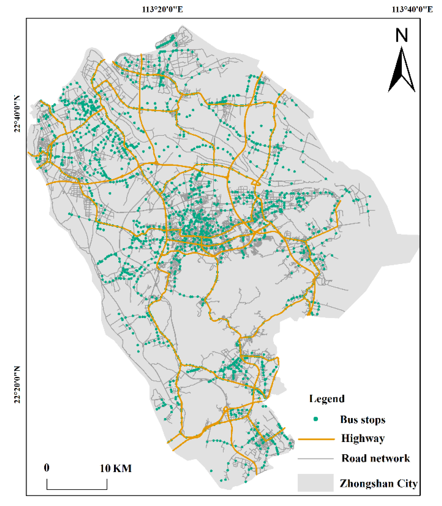
The road network dataset was obtained through the OSM project under the Open Data Commons License [42], which consists of the polylines and attributes information of road links. We also have collected the public transport network dataset (containing the location of bus stops and bus route information) from the authorities (Zhongshan Transportation Bureau, http://jt.zs.gov.cn). Bus stops were used as the ground truth, and a large proportion (98.1%) of these stops matched to a road according to their names and locations, and then the original road network was divided into RSBs based on the bus stops. Figure 4 shows the public transport network in Zhongshan City.
(2) Smart card data (SCD) and bus trajectory data
The SCD and bus trajectory data used in this study were collected from December 10 to 17, 2017. The SCD contains records only for bus passengers, and examples are shown in Table 2. For example, 328,315 and 336,077 SCD records were collected for December 10 and 11, respectively. The bus trajectory data can help recover the transport trips from the SCD, which contain a real-time sampling of the GPS positions of buses at pre-specified time intervals (about 10s~20s), along with the SCD terminal ID and bus ID (Table 3).
4.1.2. Data Preprocessing
First, to eliminate the erroneous and redundant data that are recorded in both the SCD and bus trajectory data, a data cleaning procedure was applied. During the process of passengers’ trip construction, the bus stops were used as the ground truth for matching the bus trajectory data using the method proposed by Nassir, Hickman, and Ma [43]. Examples of passengers’ trip data are shown in Table 4.
4.2. Congested RSB Estimation and Validation
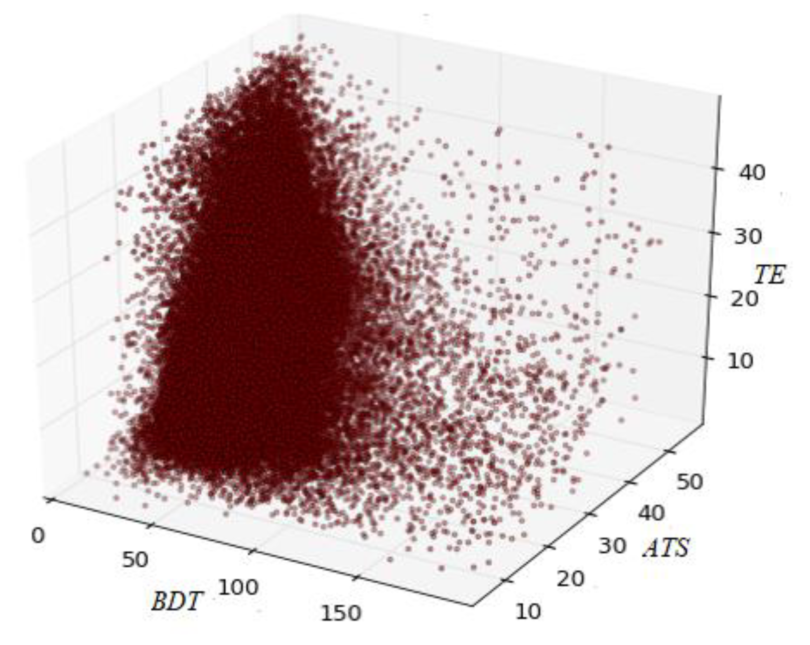
In this section, the congested RSBs were estimated from all the RSBs using the SOM algorithm. First, the three traffic indicators of an RSB (BDT, ATS, and TE) were calculated from the SCD and bus trajectory data at one-hour intervals, and the results are shown in Figure 5.
4.2.1. SOM Algorithm Results
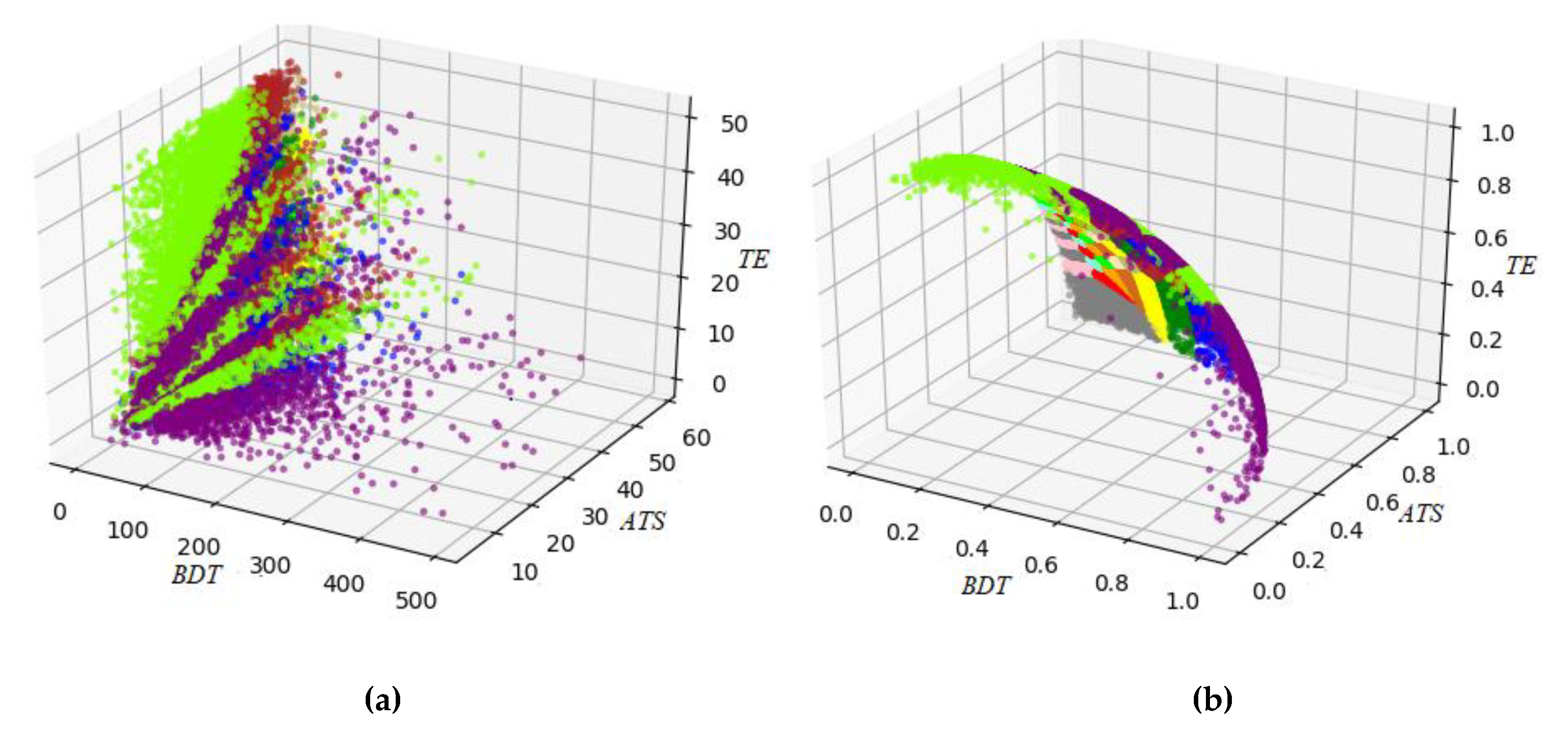
The three traffic indicators of an RSB are presented as vectors in the input space of the SOM network altogether. In this study, the optimum map sizes of SOM were chosen after several trials with different sizes, and the topographic error (TE) and quantization error (QE) were used to measure the suitability and fitness of the optimized map size [44]. When the number of neuron was 64 (8 × 8), the TE value had the local minimum value. The map size of SOM was determined as 8 × 8 in this study (Table 5). A 64-unit map (size of 8 x 8) was selected, using the 2D coordinated locations to represent the neurons and data point locations. The clustering results are shown in Figure 6.
The CISOM of each SOM cluster was calculated based on Equation (8). As a result, the congested RSBs were selected from the cluster with the maximum value of CISOM. From the data in Table 6, it is apparent that the RSBs in Cluster 0 were estimated as the congested RSBs, which include 161 RSBs.
In general, public traffic congestion is generally treated as a dynamic spatial-temporal process, in which the congested road segments are temporally approximate and spatially adjacent. The congested RSBs in this study describe the status of congested traffic for one road segment between two bus stops in one-hour intervals and are usually recurrent in the same or a similar condition. Table 7 presents examples of the detailed information for the congested RSBs. The congested RSBs were classified into three congestion levels based on a spatio-temporal analysis (Table 8). Therefore, the strategies of public transport network improvement can be designed according to the congestion level of the RSBs.
4.2.2. Validation
To validate the reliability of the congested RSBs, we calculated their ATS again using the taxi trajectory dataset. The taxi trajectory dataset has 4,757,815 records with a time interval of 30 s from December 11, 2017. The original records include the taxi ID, GPS time, longitude, latitude, direction, speed, and carry status. Only the occupied (carry status = 1) taxi trips were kept for the ATS calculation because an empty taxi could not reflect the real traffic conditions due to a slowdown for searching passengers, rest stopping or work shifting during empty trips [45]. To extract the congestion information, we need to map-match each taxi GPS trajectory, which is a sequence of discrete spatial points, to the underlying road segments. After map matching, we calculated the ATS of each RSB using a one-hour interval.
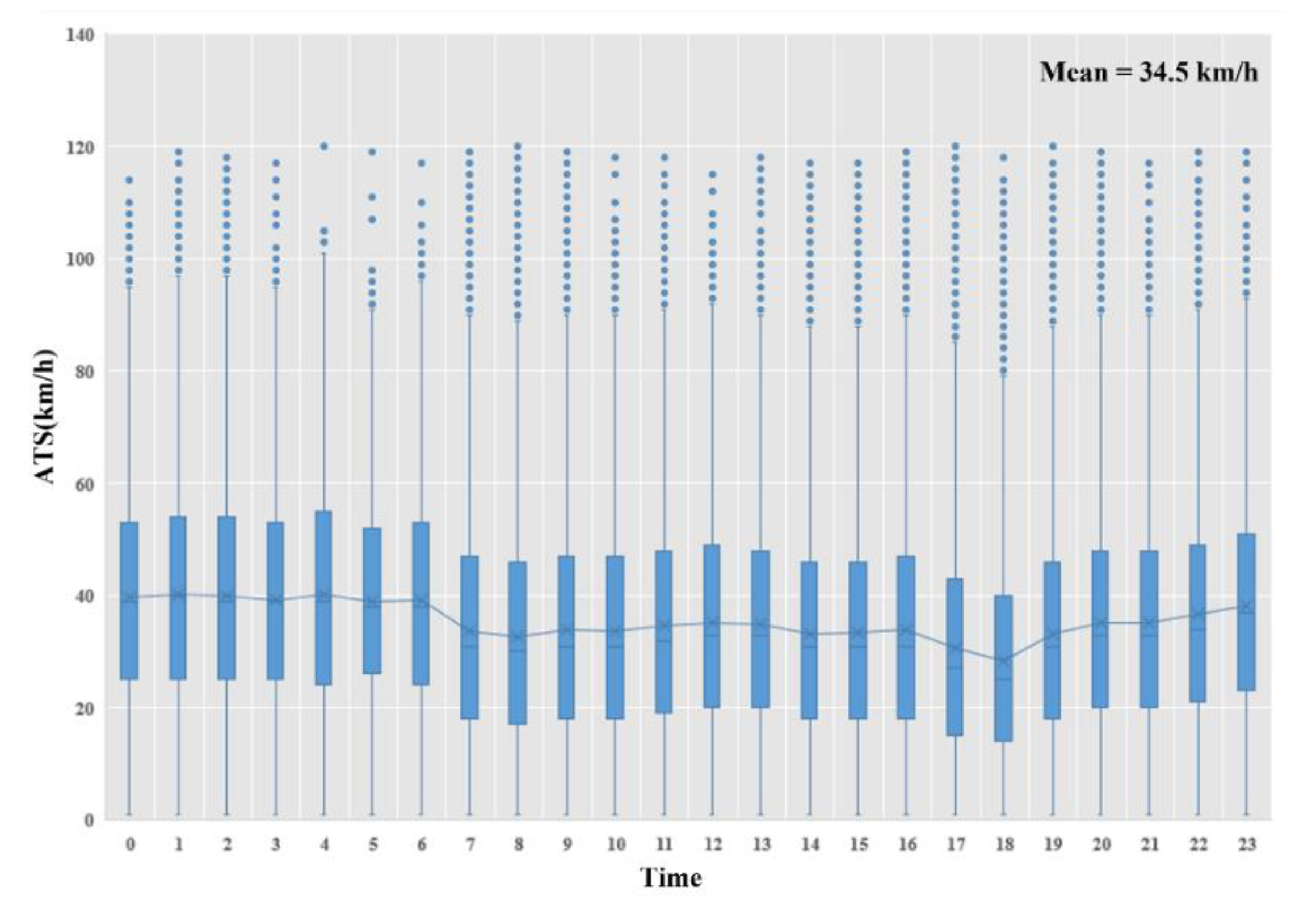
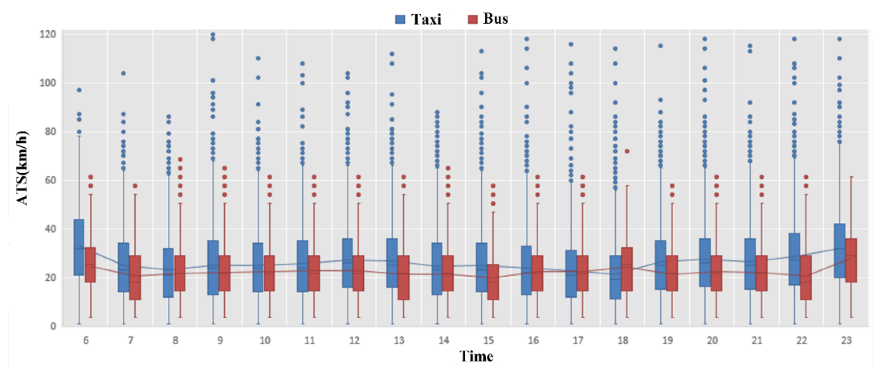
Figure 7 and Figure 8 present the boxplots and mean trends of ATStaxi for all RSBs (Mean_ATStaxi = 34.5 km/h) and congested RSBs (Mean_ATStaxi = 26.0 km/h, Mean_ATSbus = 21.8 km/h) using a one-hour interval, respectively. The average speed patterns of congested RSBs shows obvious valleys during peak commuting hours: 7:00-10:00; 17:00-18:00 (We defined the commuting hours based on [46]), which indicate the most severe traffic congestion times during a day.
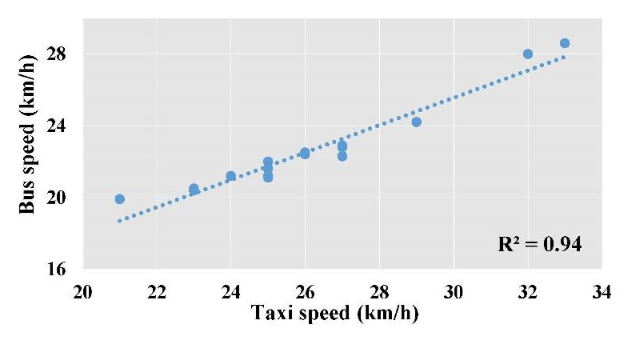
According to previous studies, the ATStaxi can be used as the primary indicator to reveal the traffic congestion of road networks [15,24,45]. The statistical correlation between ATStaxi and ATSbus of the congested RSBs is significantly strong (R2=0.94, Figure 9). This correlation pattern indicates that the congested RSBs estimated by the ATSbus are close to the results obtained by the ATStaxi, and in line with the real traffic congestion of the road network. Furthermore, in light of the statistical analysis of public transport in 2017 by the Zhongshan Public Transportation Group, the average operation speed of the buses is 21.63 km/h, which is almost in line with our Mean_ATSbus (21.8 km/h). Therefore, SCD and bus trajectory datasets used in our methodology to estimate whether the public traffic congestion of the RSBs are reasonable and effective.
5. Discussion
5.1. An Example of PTN Optimization based on Congested RSBs
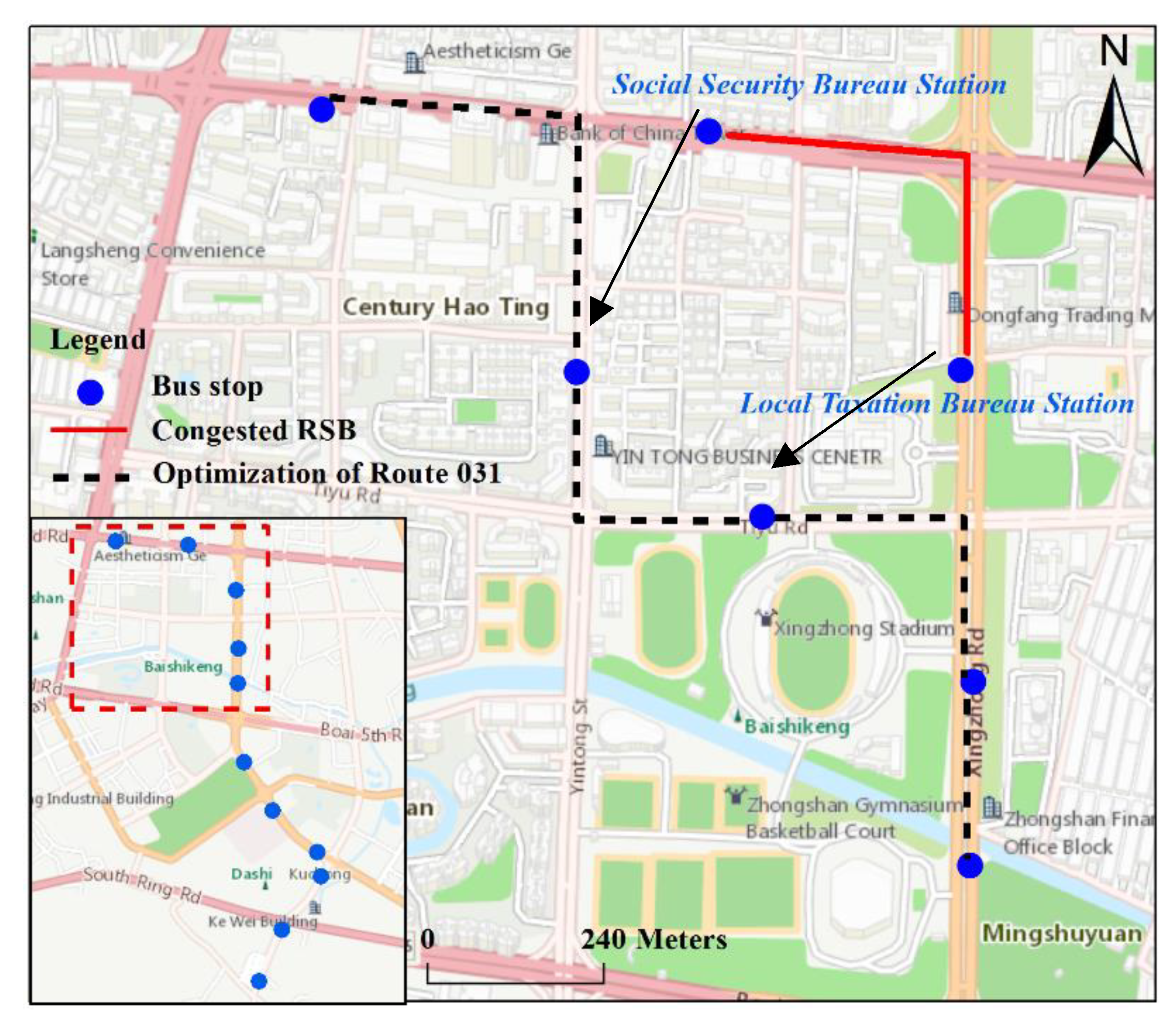
The intelligent bus stops placement of a bus line is one way to alleviate the impact of traffic congestion and thereby improve the ridership of urban public transport system. Taking bus route 031 as an example (Figure 10), the optimization measure for route 031 is to optimize the bus stop placement to avoid the congested RSB.
(1) The number of multiplexed routes: According to the Zhongshan public transport network, the number of multiplexed routes between the Social Security Bureau stop and the Local Taxation Bureau stop is 6, which are routes 024, 030, 031, 038, 216, and BRT15. The reuse of multiple bus lines is an important inducement of road congestion.
(2) Travel time: The optimization of bus stop placement can increase the bus operating speed and decrease passenger travel time by alleviating traffic congestion [11]. The travel time can be reduced by mitigating the time losses at bus stops, thereby improving the travel-time reliability of the public transport system [27].
In summary, public transport vehicles have much higher passenger capacities than private cars [47]. The placement of bus stops has been optimized for the improvement of mobility, which could moderate the headway variations and offset slight disturbances without imposing additional financial burdens.
5.2. Optimization Results Evaluating using Genetic Algorithm
To further explore the effectiveness of the PTN optimization results, we used the GA method from Nayeem, Rahman, and Rahman [48] for the optimization of bus route 031.
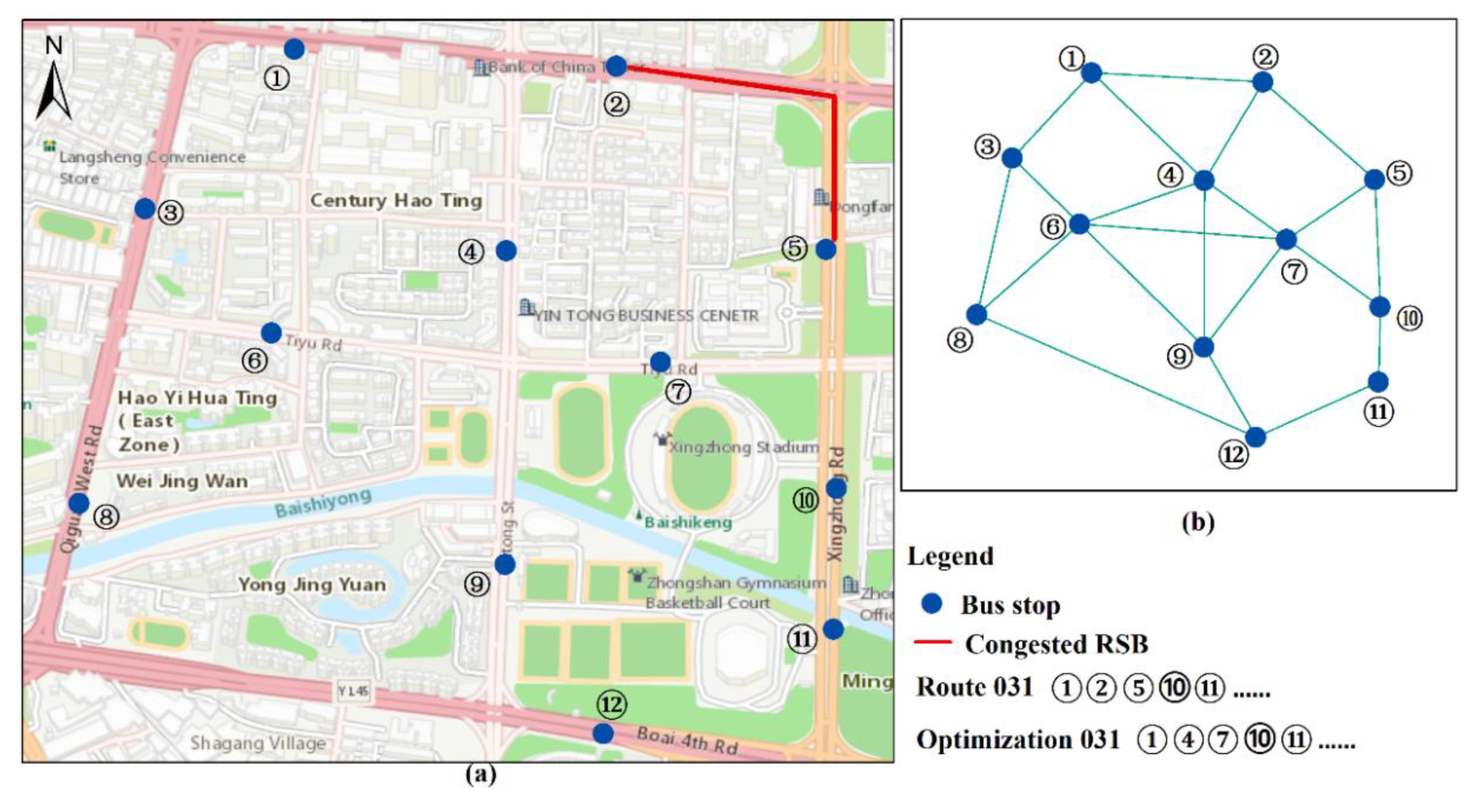
Let us consider the road network shown in Figure 11a. We described this road network by G = (N, A), where N is the set of nodes representing the bus stops, and A is the set of edges representing the RSBs. Based on the passenger trip data, we have a demand matrix denoted by dij, which represents the number of trips per time unit between node i and node j. We also denote by D the origin–destination matrix (O–D matrix) as follows:
We also know the travel time matrix for the road network denoted by trij, which represents the in-vehicle travel time between the node i and the node j. By TR, we denote the travel time matrix:
The main indicator that we use to describe the level of transport service is the total travel time spent by passengers. We calculate the total travel time of all passengers’ T in the network in the following way [48,49]:
where TT is the total in-vehicle travel time of all passengers, TTR is the total number of transfers in the transport network, TU is the total number of unsatisfied passengers (we assume that the passenger is unsatisfied when she/he has to make more than two transfers during a trip), w1 is the time penalty for one transfer, and w2 is the time penalty for one unsatisfied passenger.
T = TT + w1TTR + w2TU
Consequently, the PTN optimization could be defined as follows: for a given public transport network with n nodes, the known origin-destination matrix D that describes the travel demand among these nodes, and the travel time matrix TR, generate a set of transport routes on the network to minimize the total travel time T of all passengers.
5.2.1. Genetic Algorithm
- (1)
- (2)
- Initialization: In the initial step, each route was set as the shortest path between a selected pair of nodes according to the passenger travel time. Using the greedy algorithm from Nayeem et al. [48], we generated pairs of nodes i and j with high dsij values, which is the number of passengers that receive direct services between nodes i and j.where N is the set of nodes along the shortest path of nodes (i, j), and dmn is the passenger travel demand per time unit between nodes i and j.
- (3)
- Crossover: In the crossover operation, each gene in the individual represents a bus route. We decided at each index of the individual which one is used to perform the crossover operation between two randomly selected parents based on a given probability Pswap.
- (4)
- Mutation: Mutation is a GA operator with the goal to replace a randomly chosen gene by new genes (bus routes) in the population. Mutation usually operates with a quite small probability, which creates a slight modification of the population.
5.2.2. Results of Genetic Algorithm
A sample final solution of the GA for bus route 031 optimization is shown in Table 10. We compared the optimization of the bus stop placement of route 013 to the GA solution by considering three situations: 4 routes, 5 routes, and 6 routes. It can be clearly seen that the results obtained by GA all have at least one bus route in line with the optimization of bus route 013.
6. Conclusions
In populated urban regions, the intelligent optimization of PTN plays a prominent role in improving the transport service reliability by alleviating the unpleasant impacts of traffic congestion. In this study, we estimated the traffic congestion of the RSBs based on three traffic indicators: bus dwell time (BDT), average travel speed (ATS), and travel efficiency (TE), which were extracted from SCD and bus trajectory data. In contrast to the previous studies, which focus on the traffic status of one road segment using taxi trajectory data, the aim of our methods was to estimate the traffic congestion of the RSBs using bus trajectory data. Our methodology could be applied to estimate the congested RSBs with bus priority lanes or with limited taxi trips, which can benefit various applications including road traffic status estimation, PTN optimization, and urban transport system management. Based on the congested RSBs, the strategies of public transport network improvement are discussed and evaluated using GA. The results are expected to demonstrate the usefulness of the proposed methodology in sustainable public transport improvements.
Regarding the research limitations, our presented methodology can be applied in a city with a dominating transport mode. However, there are more public transport options (for example, metro system and tram) in major modern cities. Our future research will extend our study to mega-cities, and incorporate the impact of multiple public transport modes and complex network analysis into our methodology [50]. Moreover, the PTN optimization problem can be subdivided into two major components: the transit routing problem and the transit scheduling problem. Generally, the transit routing problem involves the development of efficient transits routes on an existing road network, with predefined pick-up/drop-off points. On the other hand, the transit scheduling problem is charged with assigning the schedules for the passenger carrying vehicles. In this context, for the PTN optimization process, future work research directions may include other fundamental variables such as bus frequency, vehicle size, function of the public transport headway, and the schedule.
Author Contributions
Yandong Wang conceived and designed the experiments; Yanyan Gu performed the experiments; Shihai Dong analyzed the data; Yandong Wang contributed reagents/materials/analysis tools; Yanyan Gu wrote the paper. All authors have read and agreed to the published version of the manuscript.
Funding
This research was funded by the National Key Research Program of China (Grant No. 2016YFB0501403); the National Natural Science Foundation of China (Grant No. 41271399); and China Special Fund for Surveying, Mapping and Geoinformation Research in the Public Interest (Grant No. 201512015).
Conflicts of Interest
The authors declare no conflict of interest.
References
- Tirachini, A.; Hensher, D.A.; Rose, J.M. Multimodal pricing and optimal design of urban public transport: The interplay between traffic congestion and bus crowding. Transport. Res. B-Meth. 2014, 61, 33–54. [Google Scholar] [CrossRef]
- Ibeas, Á.; Dell Olio, L.; Alonso, B.; Sainz, O. Optimizing bus stop spacing in urban areas. Transport. Res. E-Log. 2010, 46, 446–458. [Google Scholar] [CrossRef]
- Ibarra-Rojas, O.J.; Delgado, F.; Giesen, R.; Muñoz, J.C. Planning, operation, and control of bus transport systems: A literature review. Transport. Res. B-Meth. 2015, 77, 38–75. [Google Scholar] [CrossRef]
- Fan, W.; Machemehl, R.B. Optimal Transit Route Network Design Problem with Variable Transit Demand: Genetic Algorithm Approach. J. Transp. Eng. 2006, 132, 40–51. [Google Scholar] [CrossRef]
- LeBlanc, L.J. Transit system network design. Transp. Res. Part B Methodol. 1988, 22, 383–390. [Google Scholar] [CrossRef]
- Chakroborty, P. Genetic Algorithms for Optimal Urban Transit Network Design. Comput-Aided. Civ. Inf. 2003, 18, 184–200. [Google Scholar] [CrossRef]
- Mesbah, M.; Sarvi, M.; Currie, G. Optimization of Transit Priority in the Transportation Network Using a Genetic Algorithm. IEEE T. Intell. Transp. 2011, 12, 908–919. [Google Scholar] [CrossRef]
- Gao, P.; Liu, Z.; Tian, K.; Liu, G. Characterizing Traffic Conditions from the Perspective of Spatial-Temporal Heterogeneity. ISPRS Int. J. Geo.-Inf. 2016, 5, 34. [Google Scholar] [CrossRef] [Green Version]
- Nguyen-Phuoc, D.Q.; Currie, G.; De Gruyter, C.; Kim, I.; Young, W. Modelling the net traffic congestion impact of bus operations in Melbourne. Transport. Res. A-Pol. 2018, 117, 1–12. [Google Scholar] [CrossRef]
- Tirachini, A. The economics and engineering of bus stops: Spacing, design and congestion. Transport. Res. A-Pol. 2014, 59, 37–57. [Google Scholar] [CrossRef]
- Liu, X.; Yang, Y.; Meng, M.; Rau, A. Impact of Different Bus Stop Designs on Bus Operating Time Components. J. Public. Transport. 2017, 20, 104–118. [Google Scholar] [CrossRef] [Green Version]
- Daraio, C.; Diana, M.; Di Costa, F.; Leporelli, C.; Matteucci, G.; Nastasi, A. Efficiency and effectiveness in the urban public transport sector: A critical review with directions for future research. Eur. J. Oper. Res. 2016, 248, 1–20. [Google Scholar] [CrossRef] [Green Version]
- Chen, B.Y.; Lam, W.H.K.; Sumalee, A.; Li, Q.; Li, Z. Vulnerability analysis for large-scale and congested road networks with demand uncertainty. Transport. Res. A-Pol. 2012, 46, 501–516. [Google Scholar] [CrossRef]
- Zheng, Y.; Capra, L.; Wolfson, O.; Yang, H. Urban Computing: Concepts, Methodologies, and Applications. ACM Trans. Intell. Syst. Technol. 2014, 5, 1–55. [Google Scholar] [CrossRef]
- Yang, Y.; Xu, Y.; Han, J.; Wang, E.; Chen, W.; Yue, L. Efficient traffic congestion estimation using multiple spatio-temporal properties. Neurocomputing 2017, 267, 344–353. [Google Scholar] [CrossRef] [Green Version]
- An, S.; Yang, H.; Wang, J. Revealing Recurrent Urban Congestion Evolution Patterns with Taxi Trajectories. ISPRS Int. J. Geo.-Inf. 2018, 7, 128. [Google Scholar]
- Jenelius, E.; Koutsopoulos, H.N. Travel time estimation for urban road networks using low frequency probe vehicle data. Transport. Res. B-Meth. 2013, 53, 64–81. [Google Scholar] [CrossRef] [Green Version]
- Wang, Y.; Cao, J.; Li, W.; Gu, T.; Shi, W. Exploring traffic congestion correlation from multiple data sources. Pervasive. Mob. Comput. 2017, 41, 470–483. [Google Scholar] [CrossRef]
- Yu, Q.; Luo, Y.; Chen, C.; Zheng, X. Road Congestion Detection Based on Trajectory Stay-Place Clustering. ISPRS Int. J. Geo.-Inf. 2019, 8, 264. [Google Scholar] [CrossRef] [Green Version]
- Wang, Q.; Wan, J.; Yuan, Y. Locality constraint distance metric learning for traffic congestion detection. Pattern Recogn. 2018, 75, 272–281. [Google Scholar] [CrossRef]
- Farber, S.; Marino, M.G. Transit accessibility, land development and socioeconomic priority: A typology of planned station catchment areas in the Greater Toronto and Hamilton Area. J. Transp. Land Use 2017, 10, 879–902. [Google Scholar] [CrossRef] [Green Version]
- Kong, X.; Xu, Z.; Shen, G.; Wang, J.; Yang, Q.; Zhang, B. Urban traffic congestion estimation and prediction based on floating car trajectory data. Future Gener. Comp. Sy. 2016, 61, 97–107. [Google Scholar] [CrossRef]
- Xu, L.; Yue, Y.; Li, Q. Identifying Urban Traffic Congestion Pattern from Historical Floating Car Data. In Proceedings of the 13th COTA International Conference of Transportation Professionals (CICTP), Shenzhen, China, 13–16 August 2013; pp. 2084–2095. [Google Scholar]
- He, F.; Yan, X.; Liu, Y.; Ma, L. A Traffic Congestion Assessment Method for Urban Road Networks Based on Speed Performance Index. In Proceedings of the 6th International Conference on Green Intelligent Transportation System and Safety (GITSS), Beijing, China, 2–6 July 2015; pp. 425–433. [Google Scholar]
- Litman, T. Evaluating Public Transit Benefits and Costs; Victoria Transport Policy Institute: Victoria, BC, Canada, 2015. [Google Scholar]
- Ceder, A.A.; Butcher, M.; Wang, L. Optimization of bus stop placement for routes on uneven topography. Transport. Res. B-Meth. 2015, 74, 40–61. [Google Scholar] [CrossRef]
- Li, H.; Bertini, R.L. Assessing a Model for Optimal Bus Stop Spacing with High-Resolution Archived Stop-Level Data. Transport. Res. Rec. 2009, 2111, 24–32. [Google Scholar] [CrossRef] [Green Version]
- Chien, S.I.; Qin, Z. Optimization of bus stop locations for improving transit accessibility. Transport. Plan Techn. 2004, 27, 211–227. [Google Scholar] [CrossRef]
- Ruiz, M.; Segui-Pons, J.M.; Mateu-LLadó, J. Improving Bus Service Levels and social equity through bus frequency modelling. J. Transp. Geogr. 2017, 58, 220–233. [Google Scholar] [CrossRef]
- Nikolić, M.; Teodorović, D. A simultaneous transit network design and frequency setting: Computing with bees. Expert. Syst. Appl. 2014, 41, 7200–7209. [Google Scholar] [CrossRef]
- Wang, Y.; Zhang, D.; Hu, L.; Yang, Y.; Lee, L.H. A Data-Driven and Optimal Bus Scheduling Model With Time-Dependent Traffic and Demand. Ieee. T. Intell. Transp. 2017, 18, 2443–2452. [Google Scholar] [CrossRef]
- Yu, B.; Kong, L.; Sun, Y.; Yao, B.; Gao, Z. A bi-level programming for bus lane network design. Transport. Res. C-Emer. 2015, 55, 310–327. [Google Scholar] [CrossRef]
- Bagloee, S.A.; Sarvi, M.; Ceder, A. Transit priority lanes in the congested road networks. Public Transport 2017, 9, 571–599. [Google Scholar] [CrossRef]
- Delmelle, E.M.; Li, S.; Murray, A.T. Identifying bus stop redundancy: A gis-based spatial optimization approach. Comput. Environ. Urban. 2012, 36, 445–455. [Google Scholar] [CrossRef]
- Tirachini, A. Bus dwell time: The effect of different fare collection systems, bus floor level and age of passengers. Transp. A 2013, 9, 28–49. [Google Scholar] [CrossRef]
- Weng, J.; Wang, C.; Huang, H.; Wang, Y.; Zhang, L. Real-time bus travel speed estimation model based on bus GPS data. Adv. Mech. Eng. 2016, 8, 756467438. [Google Scholar] [CrossRef] [Green Version]
- Kohonen, T. Learning Vector Quantization. In Self-Organizing Maps; Kohonen, T., Ed.; Springer: Berlin, Heidelberg, 1995; pp. 175–189. [Google Scholar]
- Ruiz-Aguilar, J.J.; Turias, I.J.; Jiménez-Come, M.J. A novel three-step procedure to forecast the inspection volume. Transport. Res. C-Emer. 2015, 56, 393–414. [Google Scholar] [CrossRef]
- Li, Z.; Han, Z.; Xin, J.; Luo, X.; Su, S.; Weng, M. Transit oriented development among metro station areas in Shanghai, China: Variations, typology, optimization and implications for land use planning. Land Use Policy 2019, 82, 269–282. [Google Scholar] [CrossRef]
- Shieh, S.; Liao, I. A new approach for data clustering and visualization using self-organizing maps. Expert. Syst. Appl. 2012, 39, 11924–11933. [Google Scholar] [CrossRef]
- Olawoyin, R.; Nieto, A.; Grayson, R.L.; Hardisty, F.; Oyewole, S. Application of artificial neural network (ANN)–self-organizing map (SOM) for the categorization of water, soil and sediment quality in petrochemical regions. Expert. Syst. Appl. 2013, 40, 3634–3648. [Google Scholar] [CrossRef]
- OSM. Overhead Lines und Underground Cables. © Openstreetmap Contributors, Open Database License (ODbL). Available online: https://www.openstreetmap.org/copyright. (accessed on 6 September 2018).
- Nassir, N.; Hickman, M.; Ma, Z. Activity detection and transfer identification for public transit fare card data. Transportation 2015, 42, 683–705. [Google Scholar] [CrossRef]
- Kohonen, T. Self-Organising Maps; Springer: Berlin, Germany, 2001. [Google Scholar]
- Zhang, K.; Sun, D.; Shen, S.; Zhu, Y. Analyzing spatiotemporal congestion pattern on urban roads based on taxi GPS data. J. Transp. Land Use 2017, 10, 675–694. [Google Scholar] [CrossRef]
- Wu, H.; Liu, L.; Yu, Y.; Peng, Z.; Jiao, H.; Niu, Q. An Agent-based Model Simulation of Human Mobility Based on Mobile Phone Data: How Commuting Relates to Congestion. ISPRS Int. J. Geo.-Inf. 2019, 8, 313. [Google Scholar] [CrossRef] [Green Version]
- Guler, S.I.; Gayah, V.V.; Menendez, M. Bus priority at signalized intersections with single-lane approaches: A novel pre-signal strategy. Transport. Res. C-Emer. 2016, 63, 51–70. [Google Scholar] [CrossRef]
- Nayeem, M.A.; Rahman, M.K.; Rahman, M.S. Transit network design by genetic algorithm with elitism. Transport. Res. C-Emer. 2014, 46, 30–45. [Google Scholar] [CrossRef]
- Nikolić, M.; Teodorović, D. Transit network design by Bee Colony Optimization. Expert. Syst. Appl. 2013, 40, 5945–5955. [Google Scholar] [CrossRef]
- Dou, M.; Gu, Y.; Xu, G. Social awareness of crisis events: A new perspective from social-physical network. Cities 2020, 99, 102620. [Google Scholar] [CrossRef]
Figure 1.
Research framework.

Figure 2.
A general bus route.

Figure 3.
Flowchart of the self-organizing map used in this study.

Figure 4.
The public transport network in Zhongshan City.

Figure 5.
Distribution of the three traffic indicators of RSBs.

Figure 6.
(a) Clustering results of three traffic indicators for RSBs. (b) The normalized results.

Figure 7.
Average travel speed of taxis(ATStaxi) of all RSBs.

Figure 8.
ATStaxi and ATSbus of the congested RSBs (The bus operation times are 06:00-23:00).

Figure 9.
The statistical correlation between taxi speed and bus speed of the congested RSBs.

Figure 10.
The optimization of route 031. The inset shows the spatial distribution of route 031 stops.
Figure 10.
The optimization of route 031. The inset shows the spatial distribution of route 031 stops.

Figure 11.
An example of the public transport network. (a) Spatial distribution of the congested RSB. (b) Modified transport network.
Figure 11.
An example of the public transport network. (a) Spatial distribution of the congested RSB. (b) Modified transport network.


Table 1.
Example vectors of one RSB (road segment between bus stops).
| Bus Stops of the RSB | Time | BDT | TE | ATS | Vector ID |
|---|---|---|---|---|---|
| ChangHong, Minke East | 6 | 0.29542 | 0.32698 | 0.08765 | 1 |
| 7 | 0.20095 | 0.38456 | 0.07612 | 2 | |
| 8 | 0.18994 | 0.31269 | 0.08438 | 3 | |
| … | … | … | … | … | |
| 22 | 0.19742 | 0.28761 | 0.07946 | 17 | |
| 23 | 0.24765 | 0.33097 | 0.08611 | 18 |
Table 2.
Examples of the smart card data.
| ID | Card ID | Time | Route | Terminal ID | Bus ID |
|---|---|---|---|---|---|
| 1 | 920197793 | 2017/12/11 07:48:02 | 013 | 10026091 | T37925 |
| 2 | 920197876 | 2017/12/11 09:58:01 | 037 | 10029006 | T24273 |
| 3 | 920006217 | 2017/12/11 14:47:05 | 500 | 10024273 | T29006 |
Table 3.
Bus trajectory data examples.
| ID | Bus ID | Time | Longitude | Latitude | Direction | Speed(km/h) |
|---|---|---|---|---|---|---|
| 1 | T37925 | 2017/12/11 07:48:02 | 113.3108008 | 22.4562057 | 46 | 18.00 |
| 2 | T24273 | 2017/12/11 09:58:01 | 113.3203278 | 22.5557728 | 0 | 21.60 |
| 3 | T29006 | 2017/12/11 14:47:05 | 113.3255081 | 22.5612011 | 325 | 25.20 |
Table 4.
Examples of the passengers’ trip data.
| Card ID | Bus ID | Boarding Time/Stop | Alighting Time/Stop | Dist. | Time | Route |
|---|---|---|---|---|---|---|
| 920197793 | T37925 | 07:48:02/Sanjia Village | 08:02:13/Huabai Center | 2170m | 851s | 013 |
| 920197876 | T24273 | 09:58:01/Chang Hong | 10:10:22/Yangjiao Kou | 1750m | 722s | 037 |
Table 5.
Quality measures (topographic error and quantization error) of different map sizes.
| MAP Size | Normalize LOG | |
|---|---|---|
| TE | QE | |
| 4∗4 | 0.018 | 1.034 |
| 5∗5 | 0.053 | 1.047 |
| 6∗6 | 0.012 | 0.854 |
| 7∗7 | 0.043 | 0.976 |
| 8∗8 | 0.001 | 0.743 |
| 9∗9 | 0.028 | 0.712 |
| 10∗10 | 0.003 | 0.651 |
Table 6.
Results of the congested RSB estimation (top five values of CISOM).
| Cluster ID | BDT | TE | ATS | CISOM |
|---|---|---|---|---|
| 0 | 0.38692 | −0.21598 | −0.08499 | −0.08595 |
| 1 | 0.24895 | −0.29926 | −0.08056 | −0.13087 |
| 8 | 0.27386 | −0.24104 | −0.17600 | −0.14318 |
| 2 | 0.17297 | −0.32527 | −0.07892 | −0.23122 |
| 9 | 0.19913 | −0.31212 | −0.14586 | −0.25885 |
Table 7.
Examples of the congested RSBs.
| Route | Bus Stops of the Congested RSBs | Congested Periods |
|---|---|---|
| 013 | (Minke West, Zhongshan North Railway) | 07:00-09:00, 18:00-22:00 |
| 013 | (Dongming Garden, Daxinxinduhui) | 07:00-08:00 |
| 013 | (Daxinxinduhui, Sanjia Village) | 07:00-08:00, 18:00-19:00 |
| 013 | (Sanjia Village, Liantang Road) | 07:00-09:00, 18:00-22:00 |
| 013 | (Liantang Road, Zhongshan People’s Hospital) | 07:00-11:00, 17:00-22:00 |
| 013 | (Zhongshan People’s Hospital, Huabai Market) | 07:00-09:00 |
| 037 | (ChangHong, Minke East) | 07:00-09:00, 18:00-19:00 |
| 001 | (Torch College, FanZhong) | 11:00-12:00 |
| 015 | (Sun Yat-sen University, HouXing) | 08:00-09:00 |
| 031 | (Social Security Bureau, Local Taxation Bureau) | 07:00-11:00, 14:00-19:00 |
Table 8.
The congestion level of the RSBs.
| Congestion Level | Congestion Characteristic | Example Route |
|---|---|---|
| Level 1 | Recurring congestion during commuting hours | 037 |
| Level 2 | Chronic congestion on one RSB | 031 |
| Level 3 | Chronic congestion on Multi-RSBs | 013 |
Table 9.
An individual with 4 routes.
| Index | Route |
| 0 | 1-3-6-9-12-11 |
| 1 | 1-2-5-10-11 |
| 2 | 5-2-1-3-8 |
| 3 | 1-4-9-12 |
Table 10.
A final solution obtained by genetic algorithm for the transport network.
| Number of Routes | Route Description |
|---|---|
| 4 | 5-2-1-3-8-12 |
| 1-4-7-10-11-12 | |
| 1-3-6-9-12-11 | |
| 5-2-4-6-8-12 | |
| 5 | 8-3-1-4-7-10 |
| 3-1-4-7-10-11 | |
| 12-9-4-1-3-8 | |
| 9-6-3-1-2-5 | |
| 1-3-6-7-10-11 | |
| 6 | 12-8-3-1-2-5 |
| 1-3-6-9-12-11 | |
| 3-6-7-10-11-12 | |
| 1-4-7-10-11-12 | |
| 8-3-1-4-9-12 | |
| 5-2-1-3-8-12 | |
| Optimization of route 013 | 1-4-7-10-11 |
© 2020 by the authors. Licensee MDPI, Basel, Switzerland. This article is an open access article distributed under the terms and conditions of the Creative Commons Attribution (CC BY) license (http://creativecommons.org/licenses/by/4.0/).
Share and Cite
MDPI and ACS Style
Gu, Y.; Wang, Y.; Dong, S. Public Traffic Congestion Estimation Using an Artificial Neural Network. ISPRS Int. J. Geo-Inf. 2020, 9, 152. https://doi.org/10.3390/ijgi9030152
AMA Style
Gu Y, Wang Y, Dong S. Public Traffic Congestion Estimation Using an Artificial Neural Network. ISPRS International Journal of Geo-Information. 2020; 9(3):152. https://doi.org/10.3390/ijgi9030152
Chicago/Turabian StyleGu, Yanyan, Yandong Wang, and Shihai Dong. 2020. "Public Traffic Congestion Estimation Using an Artificial Neural Network" ISPRS International Journal of Geo-Information 9, no. 3: 152. https://doi.org/10.3390/ijgi9030152
Note that from the first issue of 2016, this journal uses article numbers instead of page numbers. See further details here.