Automatic Identification of the Social Functions of Areas of Interest (AOIs) Using the Standard Hour-Day-Spectrum Approach

Abstract

The social function of areas of interest (AOIs) is crucial to the identification of urban functional zoning and land use classification, which has been a hot topic in various fields such as urban planning and smart city fields. Most existing studies on urban functional zoning and land use classification either largely rely on low-frequency remote sensing images, which are constrained to the block level due to their spatial scale limitation, or suffer from low accuracy and high uncertainty when using dynamic data, such as social media and traffic data. This paper proposes an hour-day-spectrum (HDS) approach for generating six types of distribution waveforms of taxi pick-up and drop-off points which serve as interpretation indicators of the social functions of AOIs. To achieve this goal, we first performed fine-grained cleaning of the drop-off points to eliminate the spatial errors caused by taxi drivers. Next, buffer and spatial clustering were integrated to explore the associations between travel behavior and AOIs. Third, the identification of AOI types was made by using the standard HDS method combined with the k-nearest neighbor (KNN) algorithm. Finally, some matching tests were carried out by similarity indexes of a standard HDS and sample HDS, i.e., the Gaussian kernel function and Pearson coefficient, to ensure matching accuracy. The experiment was conducted in the Chongchuan and Gangzha Districts, Nantong, Jiangsu Province, China. By training 50 AOI samples, six types of standard HDS of residential districts, schools, hospitals, and shopping malls were obtained. Then, 108 AOI samples were tested, and the overall accuracy was found to be 90.74%. This approach generates value-added services of the taxi trajectory and provides a continuous update and fine-grained supplementary method for the identification of land use types. In addition, the approach is object-oriented and based on AOIs, and can be combined with image interpretation and other methods to improve the identification effect.

1. Introduction

Urban functional zoning refers to the division of regions according to the dominant functions of a city, which is an organic whole with relatively independent functions and mutual connections. Land use type refers to a land resource unit with the same land use mode, and it is the basic regional unit reflecting use, property, and distribution law. Urban areas of interest (AOIs) refer to units with a social function that attract the attention of humans. As a basic unit in urban functional zoning and land use types, the identification of the social function types of AOIs plays an important role in land use classification and urban functional partition [1,2]. The identification and renewal of urban functional zones and land use types are also hot research topics with broad applications ranging from transportation, urban planning, and smart cities [3]. However, few studies have focused on the identification of social functions of AOIs using dynamic travel data such as GPS trajectories. It is generally agreed that existing studies on the identification of land use types and urban functional zoning are mainly based on field surveys [4], remote sensing images [5,6,7,8], and social media data, such as Sina Weibo [9], Dazhong Dianping [10], Twitter [11] and points of interest (POIs) data.

Methods based on field surveys currently have the highest spatial accuracy, but these methods are time-consuming and unproductive. For example, the Third National Land Survey Project in China will be completed in two years, while the previous two works can be traced back to 2009 and 1996 [4]. There are many remote sensing images for land use recognition, including nighttime light images [12], Landsat images [13], and hyperspectral images [14]. Due to their low spatial resolution, nighttime light images are more suitable for estimating built-up areas and building density on large scales [15]. Even the new satellite, Luojia1-01, only has a spatial resolution of 130 m [12]. Landsat is widely used as a free global data source. However, since it is limited by a spatial resolution of 30 m and a re-sampling period of 16 days, the space-time application of its data can only be at the block level, of which the recognition efficiency of hyperspectral images is much better than that of Landsat [16]. However, the slow processing speed and the Hughes phenomenon, which are caused by the multi-dimension of images, restricts the wide application of hyperspectral technology [17]. In general, the classification of remote sensing images is based on pixels. Even object-oriented methods can only be used to identify homogeneous objects [18]. However, when the object is composed of multiple spectral features, there are difficulties in the recognition process.

Studies of functional zone identification based on POI data have also begun to appear recently, mainly focusing on the classification of POIs [19], analysis of the density and spatial distribution of specific types of POIs, and functional partitions combined with remote sensing images [20]. The major limitation is that some POIs are acquired based on volunteered geographic information, and the quality of the data is hard to guarantee [21]. Studies have shown that traffic patterns are closely related to urban functional zoning [22,23]. Population mobility and travel behavior are essential themes in sociology, geography, and transportation [24,25]. It is generally agreed that human activities have strong regularities, and most of these are predictable [26,27]. For example, the spatiotemporal attenuation of large-scale travel follows a power-law distribution or an exponential truncated power-law distribution [28,29], while a single trip mostly follows an exponential distribution [30]. At the same time, the first law of geography by Tobler is equally applicable to the law of human travel [31], which also shows certain regularities, such as distance decay in space [32].

Apart from the abovementioned data sets, travel data such as currency data [28], mobile phone data [29,33], subway bus card data [34] and floating car data [35,36] are widely used in the analysis of travel behaviors. Among these, the trajectory data of taxicabs record the spatial location more closely to the destination, which is more suitable for fine-grained research. The most frequently used methods of trajectory data sets include hot spot discovery methods, such as Getis-Ord(Gi* statistic) [37] and (kernel density estimation (KDE) [38], and various spatial clustering algorithms and their optimization [39], such as k-means [40] and k-medoids [41] based on division, or density-based spatial clustering of applications with noise (DBSCAN) [38] or clustering by fast search and find of density peaks (CFSFDP) [42] based on density. Existing studies provide theoretical and methodological knowledge for the description of travel behavior laws [43,44], which is an important component in urban functional zoning studies. Combining these advanced analysis methods with taxi trajectories and applying them to social function type identification of the AOIs can provide a more precise and accurate analysis [45,46,47].

Extraction of the pick-up and drop-off points from the raw trajectory is a refined process from the perspective of travel behavior. Clusters of the pick-up and drop-off points are usually the origin or destination of human mobility, and the locations of these clusters are often close to some AOIs. From a time perspective, if we count the traffic flow per hour in days, we will draw an hour-day-spectrum (HDS). Each cluster has six types of HDS, including total drop-offs, holiday drop-offs, weekday drop-offs, total pick-ups, holiday pick-ups, and weekday pick-ups, which reflect the time change regularity of travel behavior. By matching all of the waveforms of each cluster with the standard HDS of each AOI type, we can automatically identify the social function types of the AOIs.

The main innovations of this article include:

(1) Data preprocessing of double cleaning. After cleaning twice, the spatial accuracy of the pick-up and drop-off points is ensured; this is better for micro-level travel behavior analysis. This operation leapfrogs travel research from macro to micro, from city level to block-level, and from community level to building level. The buffer analysis combined with DBSCAN automatically classifies the pick-up and drop-off points. Each cluster can be automatically associated with a neighboring AOI to determine the affiliation of the points with the AOI.

(2) A top-down method of automatic identification of AOI is designed. This method relies on the six types of HDS of AOIs. The standard HDS of the AOI is obtained by temporal analysis on the pick-up and drop-off points, and then the social function of the AOI is identified by the spectrum matching technique.

(3) Waveform recognition is obtained using the HDS pattern matching method of the Gaussian kernel function. Compared with the method based on the cosine similarity and the Pearson correlation coefficient, the recognition accuracy is obviously improved, and the rate is increased to 90.74%.

This method requires only the trajectory data of the taxicabs, and automatic identification of the functional type can be performed without adding new sensors and data sources. Because the trajectory in each city is continuously being updated in intelligent transportation systems (ITS), the implementation of this scheme can achieve long-term and dynamic monitoring of the social functions of AOIs. The results can be used alone or in combination with other schemes to complement the urban functional area identification.

The rest of the article is arranged as follows. Section 2 presents the methodology. The study area and data preprocessing, as well as results and analysis, are introduced in Section 3. Then, discussion occurs in Section 4. Lastly, conclusions and future work are covered in Section 5.

2. Methodology

AOI can be regarded as an important part of land use types, and the identification of its social function type is a hot topic. This article attempts to identify the social function types of AOIs through the spatiotemporal data mining of taxi GPS trajectories. This section will introduce the principle and implementation of the supervised classification method in detail.

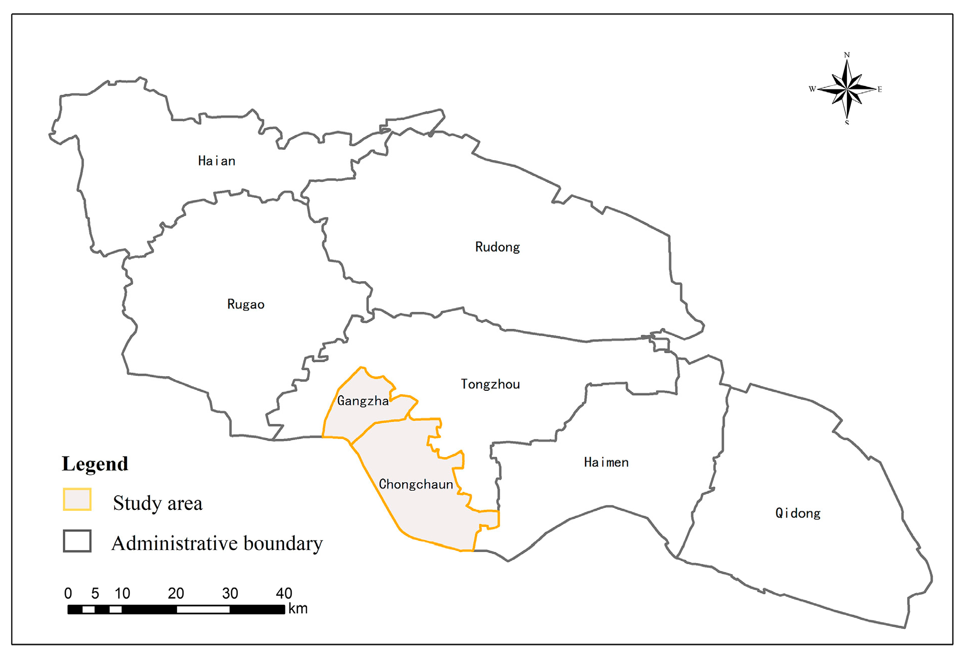
2.1. Study Area

The study area is presented in Figure 1. All experiments were conducted in the Chongchuan and Gangzha Districts, which cover about 234 square kilometers, and the permanent population was 0.884 million in 2017. These districts are the traditional main urban areas of Nantong, and Nantong is the prefecture-level city in Jiangsu Province, China. It is located on the northern bank of the Yangtze River. In 2018, Nantong had a gross domestic product growth of 8.95%, with a total of about 842.7 billion yuan, ranking 20th across the whole country. Because the subway in Nantong has yet to be constructed, buses and taxis are the main travel ways of urban human mobility in public transportation. Taxis play an important role in citizens’ lives. The total number of taxis in Nantong is about 1200 and the number of buses is about 3000.

2.2. Research Framework

Figure 2 illustrates the research framework and interrelated tasks of this proposed work, with the details given below.

• Extraction and cleaning of the pick-up and drop-off points of the taxi GPS trajectories. First, anomalous data with the wrong spatial position or an empty value are removed, and then the drop-off points are cleaned again to improve the spatial accuracy.
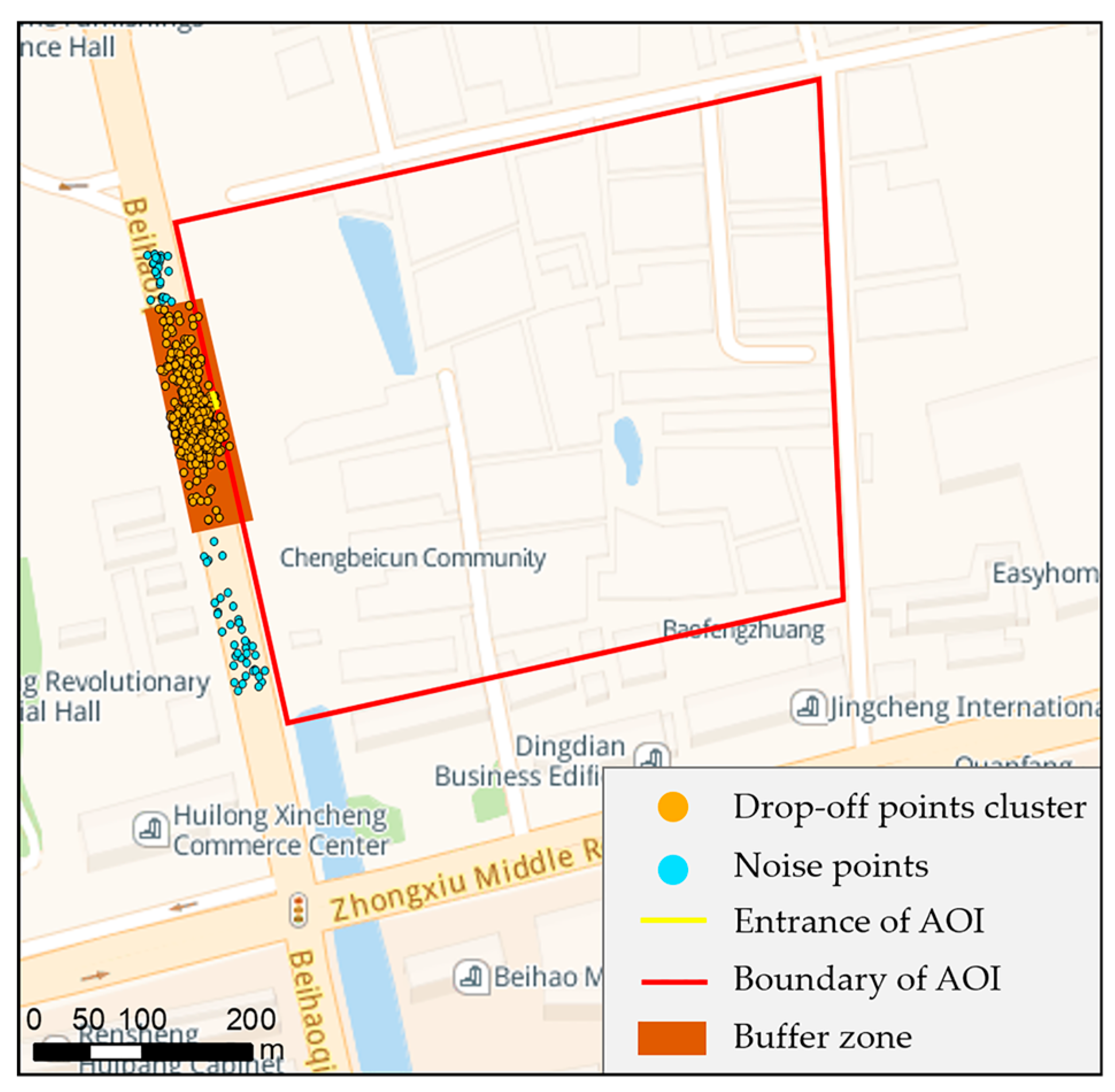
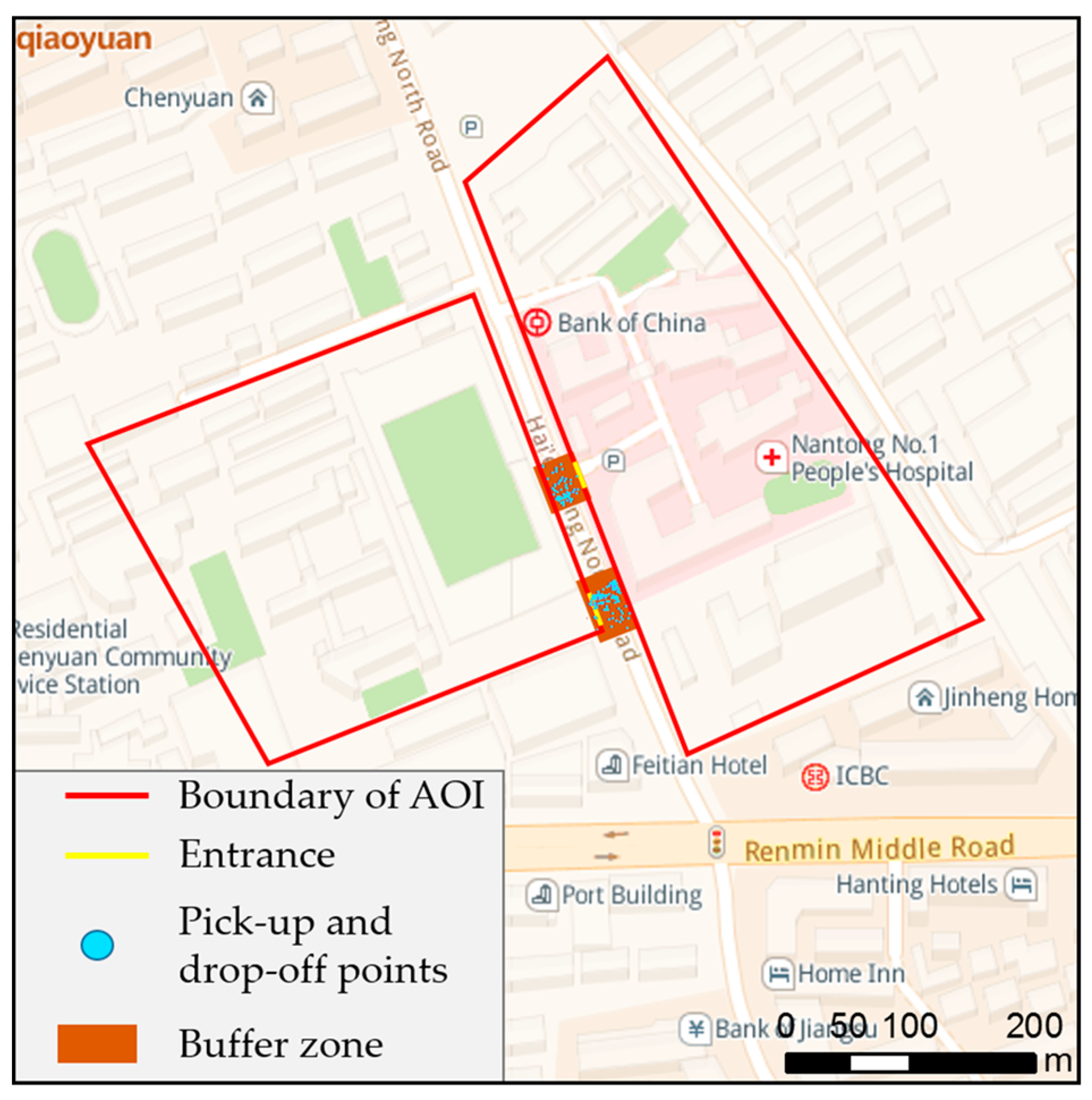
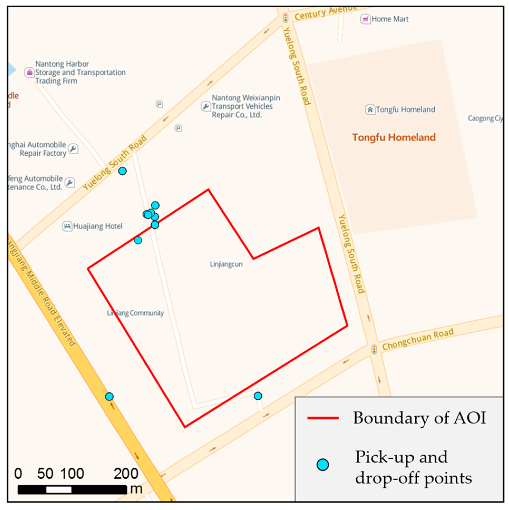
• Associating the AOIs with pick-up and drop-off points. First, the buffer analysis and DBSCAN are combined to extract the taxi pick-up and drop-off point clusters. DBSCAN and spatial buffer analysis are used for AOI entrances with closed management, while buffer analysis is used for AOI entrances with open management. Finally, the pick-up and drop-off points are associated with AOIs.
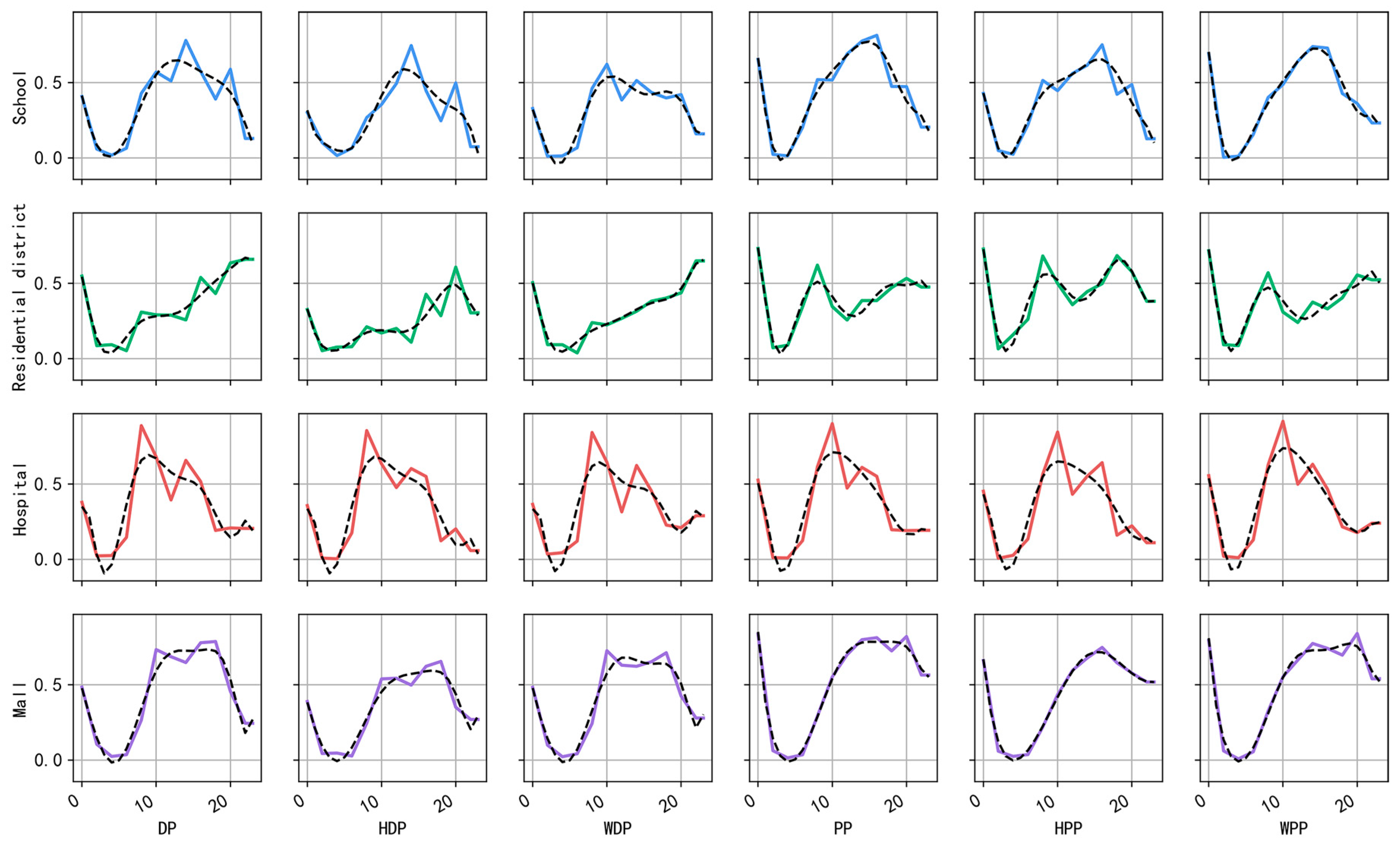
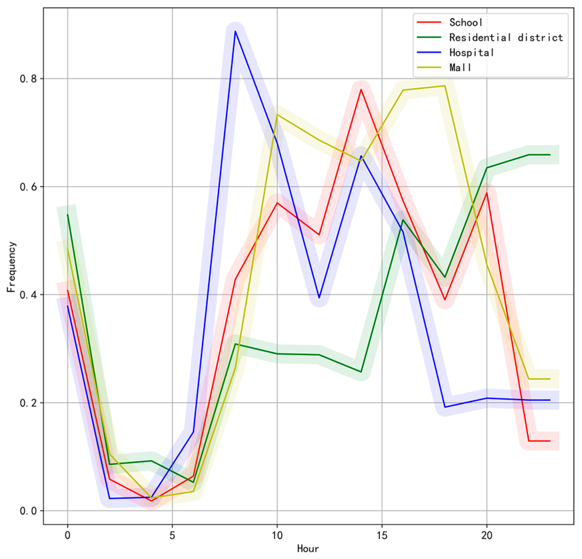
• Training of six standard hour-day-spectra (SHDSs) of each AOI type.
• Identification of social functional type of AOIs according to standard HDS with the KNN algorithm.
• Validation of the methodology using real data.

2.3. Associating AOIs with Pick-Up and Drop-Off Points

Compared to other public travel modes, the taxi is the most maneuverable and flexible, and its drop-off points are relatively close to the destination. Based on different methods, the collections of drop-off points near AOI entrances were collected as sample data. We used DBSCAN combined with spatial buffer in closed entrances analysis, as well as spatial buffer singly in open entrances.

The road boundaries constrain the distribution of the drop-off points, so the setting of the buffer size should vary according to the width of each road. Because the spatial error of the GNSS device was five to ten meters, in order to include more drop-off points into the buffer zone, the buffer width perpendicular to the road was determined by adding ten meters to the road width.

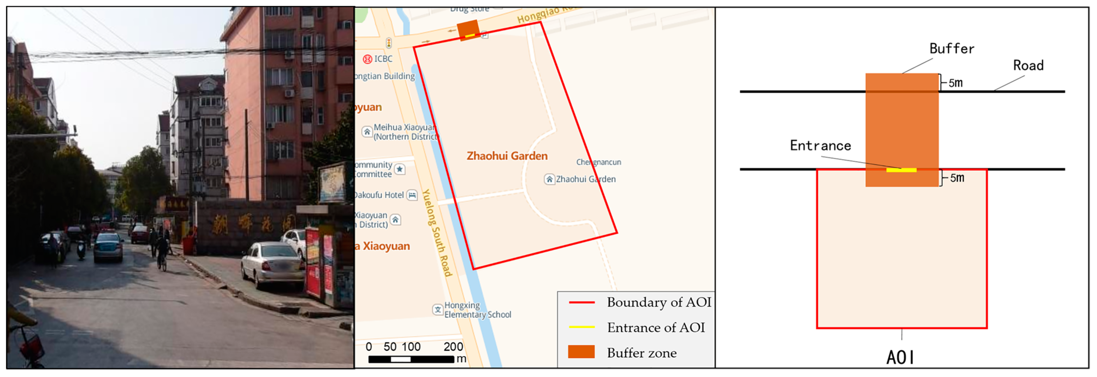
2.3.1. Closed Entrances

Closed entrances have doorplates, gateposts, fences, and other iconic objects, so we carried out DBSCAN clustering for pick-up and drop-off points in the buffer, removed noise points in the results, and then associated the pick-up and drop-off point clusters with AOIs. Combined with buffer analysis, we determined buffer widths parallel to the road by using the drop-off point density associated with AOIs, as shown in Figure 3.

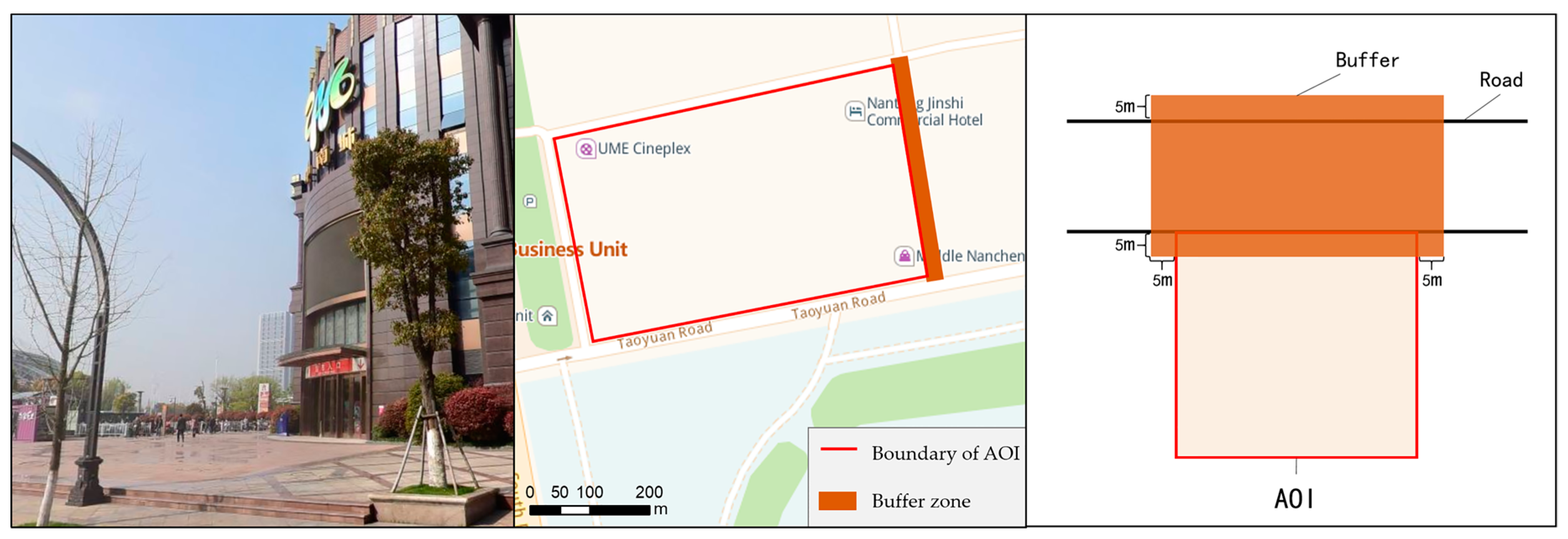
2.3.2. Open Entrances

Some AOIs, such as shopping malls, have no clear accessible entries, which means people can enter or leave the area from any position along the road. To eliminate GPS data error, buffer widths parallel to the road were obtained by adding ten meters to the AOI boundary length, as shown in Figure 4.

2.4. Training of SHDS for Each Type of AOI

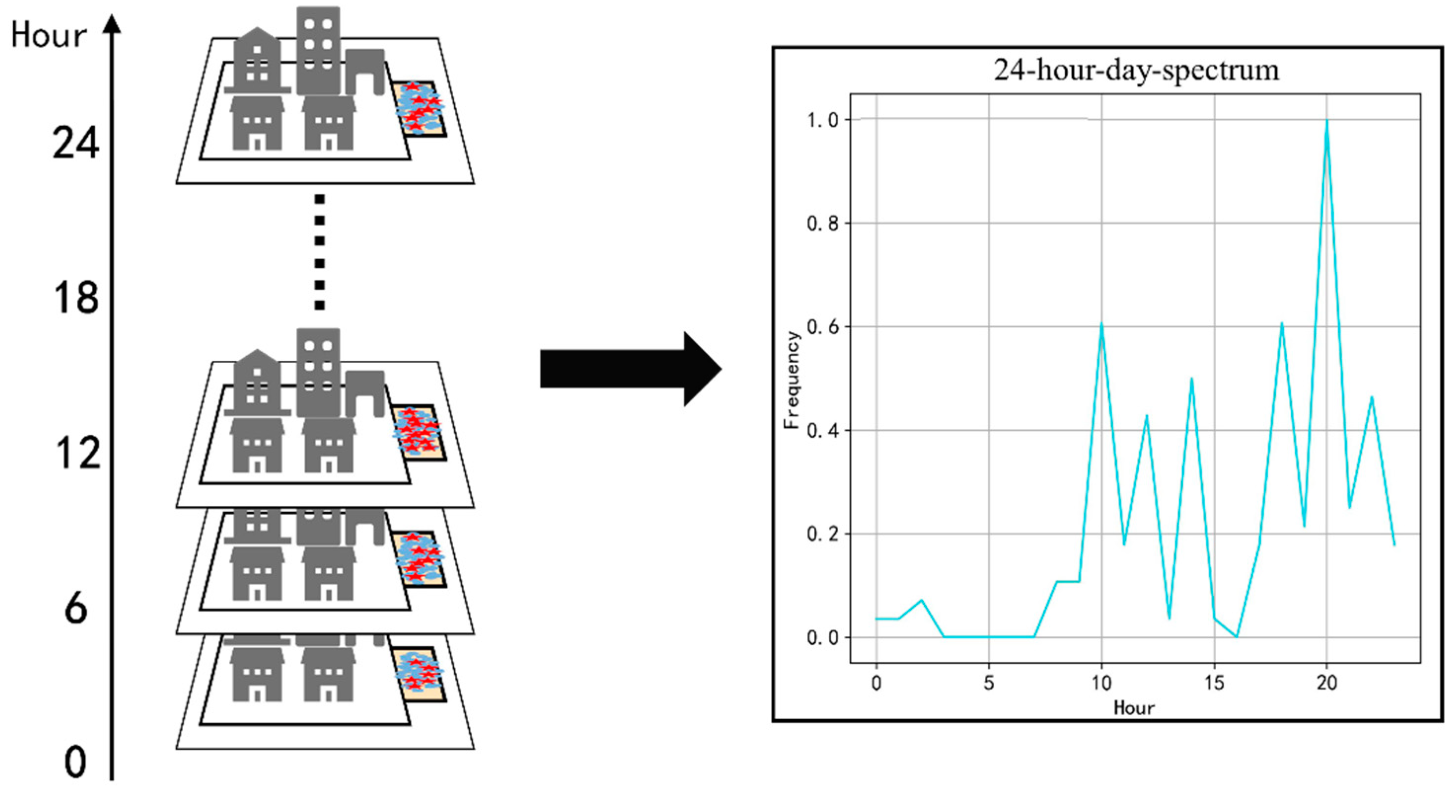
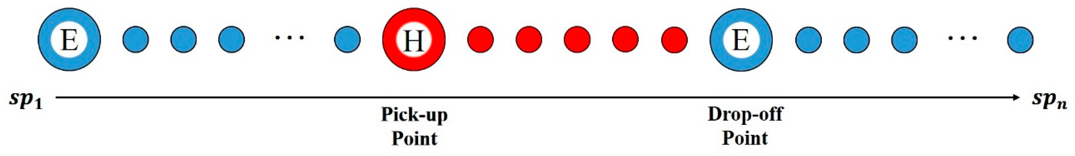
2.4.1. Conception of SHDS

There are several types of AOIs, but for a specific type, the composition of the population is relatively similar, and, therefore, people tend to travel short distances. This means that the temporal distribution law of the same type of AOI is similar. Daily, there are differences between weekdays and holidays. For example, primary and secondary schools are only open on weekdays, but the scenic spots attract more tourists on Sundays. Hospitals have no rest all year round, having a relatively balanced distribution of people flow. In the HDS, some AOIs have several peaks in a day. For instance, students have a fixed school time, which results in corresponding morning and evening peaks in residential districts. The differences between functional zones, like a person’s unique fingerprints, can be used to identify the different types.

The flow of passengers can be expressed by the number of pick-up and drop-off points near the AOI entrance. Hence, the spectrum constructed by these points in each time period is a sign of the AOI’s own characteristics. From a time point of view, HDS includes differences between holidays and weekdays. At the same time, HDS includes differences between pick-up and drop-off points. Thus, HDS can be divided into six types, including total drop-offs, holiday drop-offs, weekday drop-offs, total pick-ups, holiday pick-ups, and weekday pick-ups. The above characteristics can be described as curves in a two-dimensional coordinate system, that is, the horizontal axis represents 0–23 o’clock, and the vertical axis represents the flow of people, which is called HDS in this paper.

Because same types of AOIs have similar social systems and working characteristics, their own characteristics are almost identical. Under this circumstance, it is possible to use a standard spectrum to identify the characteristics of such AOIs. Corresponding to the aforementioned six types of HDSs, six types of standard spectrum can be generated which are collectively called SHDSs.

2.4.2. Implementation

The SHDS should express the fundamental law of all AOIs in this type. Hence, information of only one example is taken, as the SHDS has greater subjectivity and deviation. In order to acquire a SHDS with strong universality and distinction, this paper uses a method based on sampling and interpolation. The implementation process is as follows:

(1) We extract the pick-up and drop-off points in each buffer of the AOI entrance. In addition, according to the ‘Time’ field, the number of hourly points within 24 h is separately counted to calculate the time-interval spectrum, as shown in Figure 5.

Distribution of the pick-up and drop-off points is usually uneven; the region close to the AOI entrance may have a high density. The DBSCAN algorithm is sensitive to the distribution density of points, which can extract the clusters of the points and remove noise points. Because the parking position of the vehicle is dispersed around the closed entrance, the DBSCAN algorithm is used to cluster the pick-up and drop-off points in the buffer, as shown in Figure 6.

Then, after extracting the quantity sequence of pick-up and drop-off points, the data set can be divided into the following: PP = {${pp}_1,{pp}_2,\dots ,{pp}_n$} represents pick-up points, HPP = {${hpp}_1,{hpp}_2,\dots ,{hpp}_n$} represents pick-up points on holidays, WPP = {${wpp}_1,{wpp}_2,\dots ,{wpp}_n$} represents pick-up points on weekdays, DP = {${dp}_1,{dp}_2,\dots ,{dp}_n$} represents drop-off points, HDP = {${hdp}_1,{hdp}_2,\dots ,{hdp}_n$} represents drop-off points on holidays, and WDP = {${wdp}_1,{wdp}_2,\dots ,{wdp}_n$} represents drop-off points on weekdays.

(2) By calculating the spectrum of AOI with sequence data, the spectral sequence ${HDS}_j^{\left(k,h\right)}$ is {s₁, …, s_i, …, s₂₄}, where i is the sequence number of the spectrum (1 ≤ i ≤ 24), j is the number of examples, k is the number of classes, h is the number of spectral types, s_i is the quantity of pick-up and drop-off points at time i, and ${HDS}_j^{\left(k,h\right)}$ represents the spectral information of the jth example of the kth class of AOI and the hth class of the spectrum.

(3) The average hour-day-spectrum ${AHDS}^{\left(k,h\right)}$ is calculated for each type of AOI, as shown in

$${AHDS}^{\left(k,h\right)}=\frac{1}{N}{\displaystyle \sum _{j=1}^N}{HDS}_j^{\left(k,h\right)}$$

(1)

where N is the total number of examples of the kth class.

(4) The same type of HDS may sometimes have abnormal values, that is, the spectral shape shows sharp fluctuations. It is therefore necessary to take interval sampling for ${AHDS}^{\left(k,h\right)}$ with m to reduce the influence of abnormal values. The result ${Resample}^{\left(k,h\right)}$ is {s₁ …, s_i+m, …, s₂₄}. In order to ensure the universality of SHDSs and retain the distinction of the original HDS, m is less than 3.

(5) The dimension of the spectrum after sampling is less than 24, but the HDS of the AOI to be identified is 24 dimensions. Thus, it is necessary to interpolate the ${Resample}^{\left(k,h\right)}$ sequence to restore it with 24 dimensions, and the interpolation result is the final standard spectrum ${SHDS}^{\left(k,h\right)}$.

2.5. Automatic Identification of Social Function of AOIs with KNN and SHDSs

KNN is a common method used in data mining classification technology. Compared with other machine learning algorithms, it is especially suitable for multi-classification processing. However, it has a large time complexity when calculating the similarity between the sample and all training samples. Hence, the SHDS is used to replace the whole sample set; this means only the overall similarity (distance) of the HDS and the corresponding SHDS needs to be calculated, which can greatly reduce the algorithm complexity.

2.5.1. Concept of KNN

KNN means that the nearest k neighbors can represent each sample. If a sample has a majority of the k nearest neighbors belonging to a certain type in the feature space, the sample is also classified into this type. In the KNN algorithm, the selected neighbors are considered to have been correctly classified. The classification decision only depends on the type of the nearest one or several samples.

The following steps are performed for each point in the dataset of an unknown type:

• The distance is computed between the point in the known type and the current point;
• The distances are sorted in ascending order;
• k points with the smallest distance from the current point are chosen;
• The occurrence frequency of the type of the first k points is obtained;
• The type with the highest frequency as the classification of the current point is returned.

2.5.2. Combination of KNN and SHDS

There are differences between different types of HDSs of the same AOI, and the same type of HDS of different AOI types may also be different. However, for a specific type of AOI, the shape of the six HDSs is relatively stable, meaning the spectral curves can be assembled and regarded as the identification of the AOI type. The number of pick-up and drop-off points near the entrance is recorded in the spectrum sequence. However, due to the differences in acquisition time and spatial regions, the error is high when calculating the similarity of the spectral sequence based on the absolute number, and the spectral sequence elements need to be normalized in advance. The steps of the identification method are as follows:

• The training process of the SHDS
  The spectrum sequence is converted into a 24-dimensional vector and normalized, and then six SHDSs of various types of AOIs are calculated. The normalization formula is

  $$\mathrm{v}\prime =\frac{v-v_{min}}{v_{max}-v_{min}}$$

  (2)

  where $v$ denotes the vector form of this type of SHDS, $v_{min}$ denotes the minimum value of the vector, and $v_{max}$ denotes the maximum value of the vector.
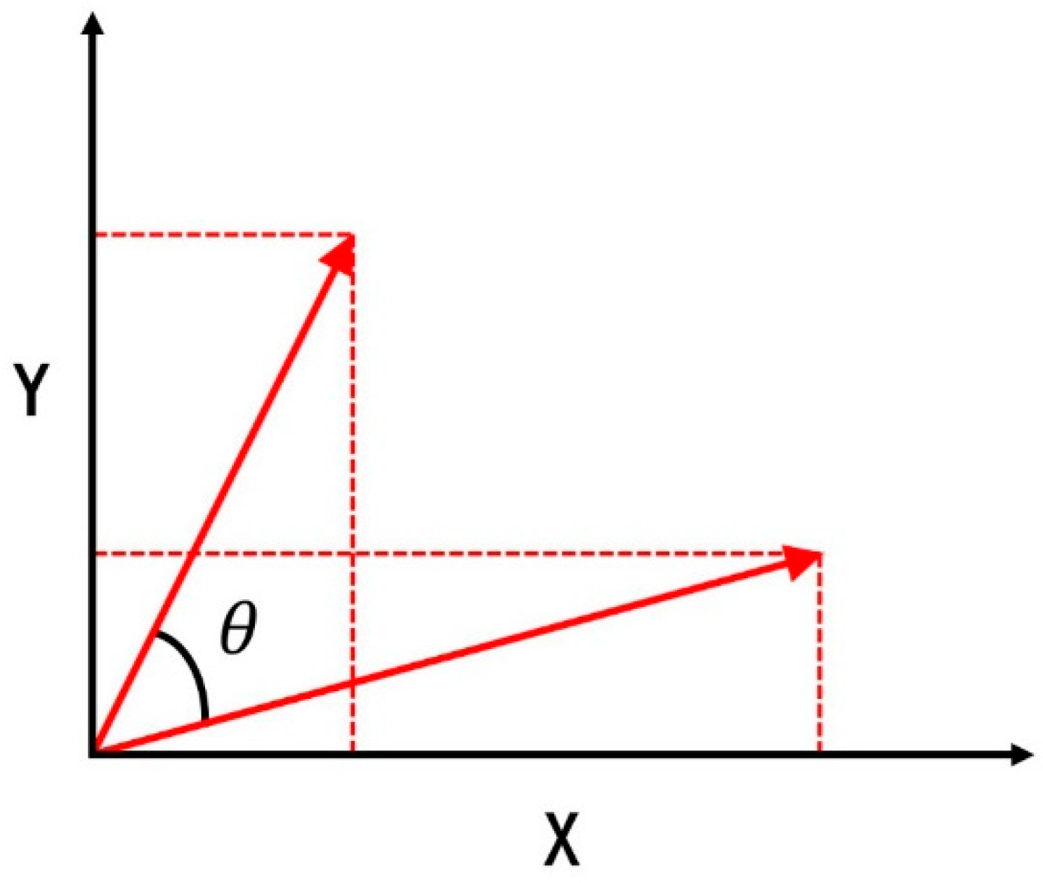
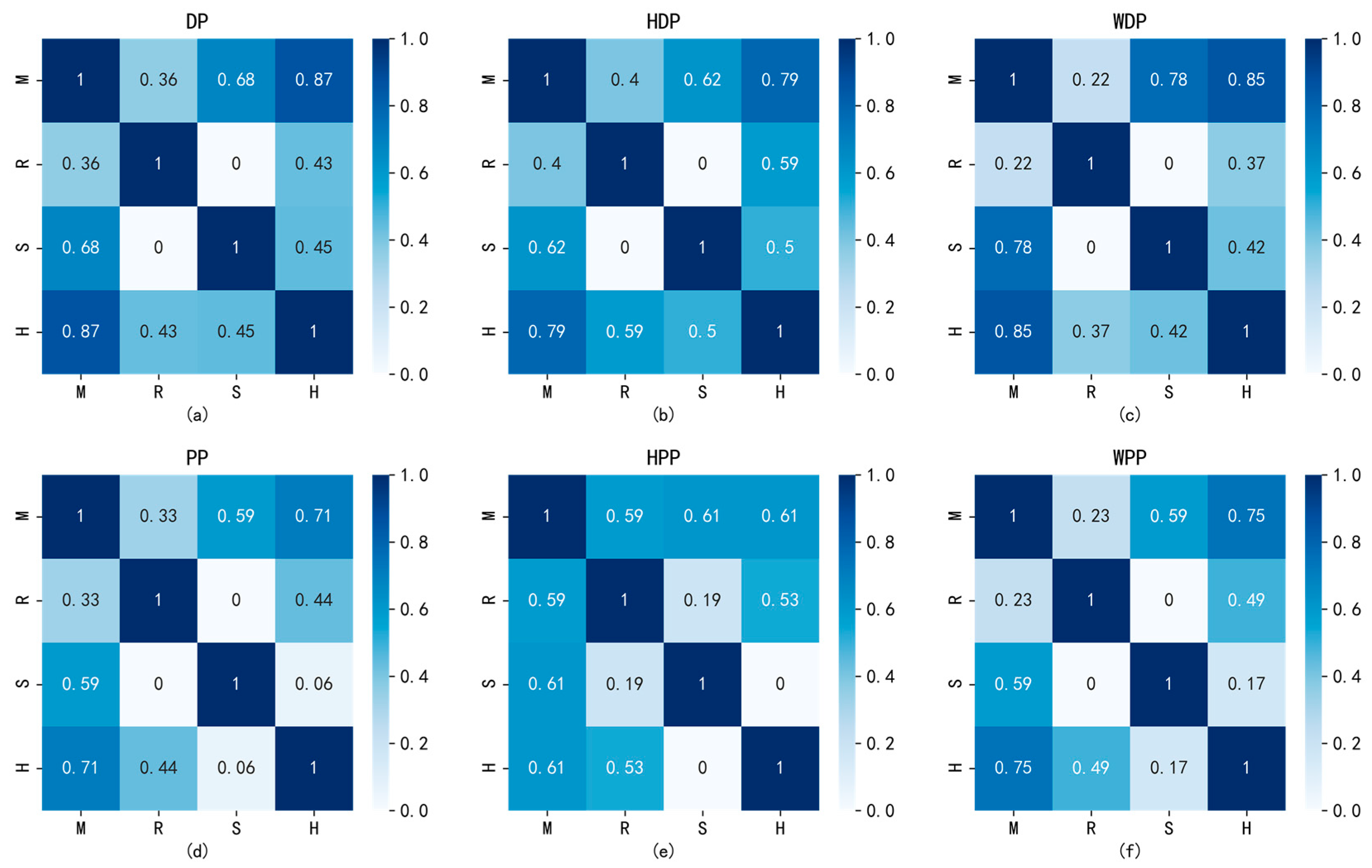
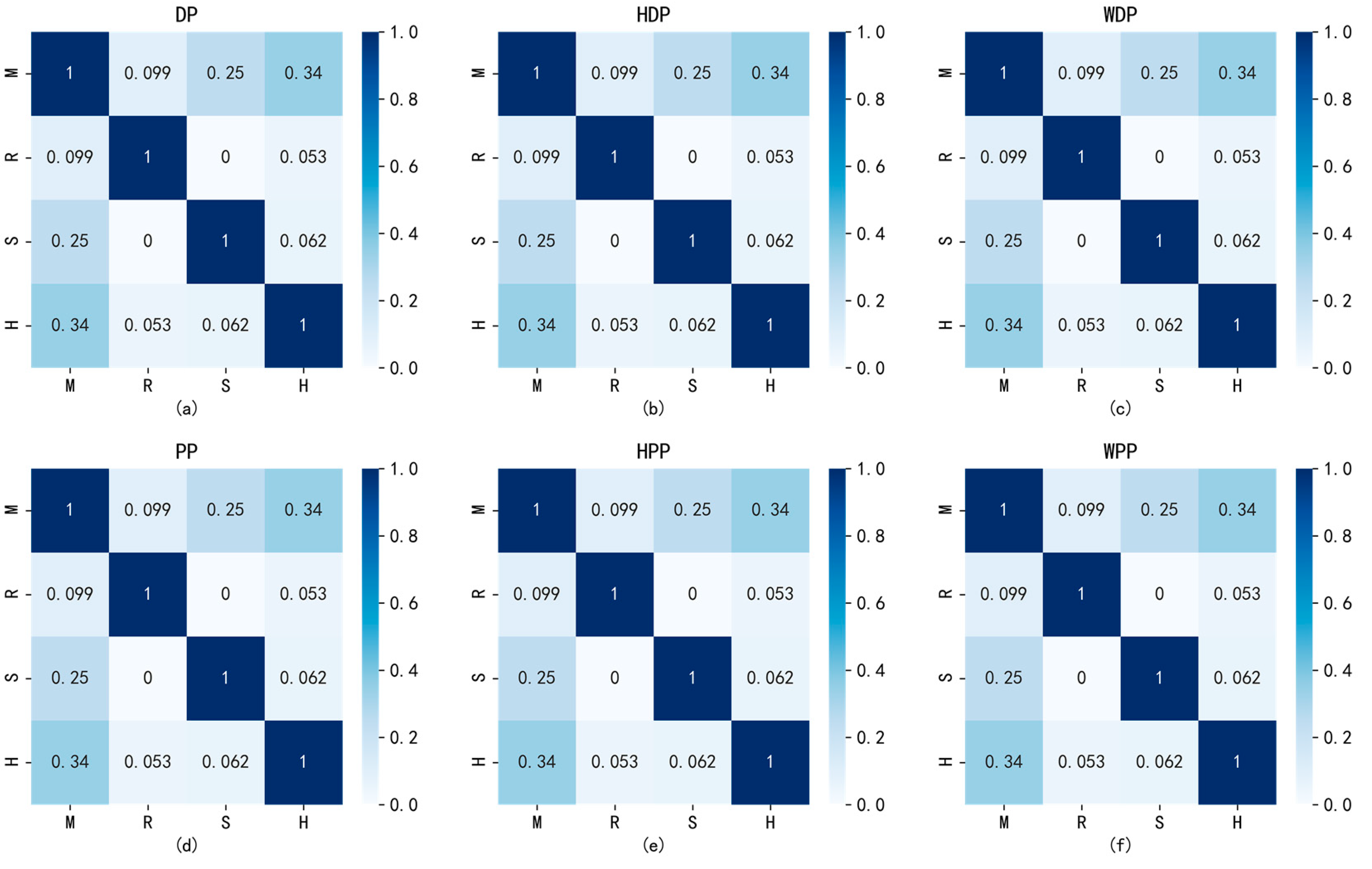
• Identify the type of AOI
  Cosine similarity, Pearson coefficient, and Gaussian kernel function were selected as the similarity (distance) functions of KNN, respectively, and the best one was decided according to the sensitivity of self-correlation of the AOIs’ SHDSs.
  The next step involves converting the AOI spectrum sequence to be identified into a normalized vector form, calculating the similarity with the SHDS vector of each type, integrating the six spectral similarities, and calculating the total similarity as the distance factor in the KNN algorithm. The calculation formula is

  $${corr}_{type\_i}^k=Similarity({SHDS}_{type\_i}^k,{HDS}_{type\_i})$$

  (3)

  $$s^k={corr}_{type\_1}^k+{corr}_{type\_2}^k+{corr}_{type\_3}^k+{corr}_{type\_4}^k+{corr}_{type\_5}^k+{corr}_{type\_6}^k$$

  (4)

  where $k$ denotes the index of the AOI types, $type\_i$ denotes the type of spectrum (for example, the spectrum of weekdays), ${Corr}_{type\_i}^k$ denotes the similarity between the SHDS of type_i and the HDS to be identified; and $s^k$ denotes the total similarity between the $HDS$_k and $SHDS$.

3. Result and Analysis

In order to validate the feasibility of the approach, 108 AOI samples were selected as test sets, and different similarity calculation methods were used to verify the results.

3.1. Study Area and Data Preprocessing

3.1.1. Trajectory Data of the Taxi

The original taxi GPS trajectories data involved about 1,400 taxis from September to October 2018 in Nantong, China, of which the attributes included the license plate number, the driver’s call sign, and latitude and longitude, etc., as shown in

Table 1. Origin trajectory sample data of taxis.

License Plate Number	Call Sign	Time	Latitude and Longitude	Speed	Direction	State
SU FB3451	13646244156	1 September, 2018 0:00:00	120.840075, 32.136626	16.7	Northeast	Empty
SU FB3451	13646244156	1 September, 2018 0:00:30	120.841270, 32.137205	12.5	Northeast	Empty
⁝	⁝	⁝	⁝	⁝	⁝	⁝
SU FB3451	13646244156	1 September, 2018 23:59:00	120.818281, 32.071339	22	Southeast	Empty
SU FB3451	13646244156	1 September, 2018 23:59:30	120.820179, 32.069533	26.1	Southeast	Heavy

. Specifically, ‘Time’ indicates the time at which the trajectory point is recorded, ‘Latitude and longitude’ represent the current geographic location of the vehicle, ‘Speed’ records the current vehicle speed, and ‘Direction’ signifies the current direction. If ‘State’ is left empty, this indicates that there are no passengers in the car.

The designed sampling time interval was 30 s, but it was less than 30 s in practice because the signal data caused by the change in passenger status were also collected. We then extracted information on the pick-up and drop-off points according to the vehicle state. When the state of the vehicle changes from empty to heavy, this is the pick-up point, and vice versa, as shown in Figure 7.

In practice, taxi drivers change the passenger status after passengers get on, leading to a relatively small error between the recorded pick-up point and the actual pick-up point. However, when approaching the destination, some drivers will change the status in advance, resulting in a significant error between the recorded drop-off point and the actual recorded drop-off point. Hence, this paper characterizes the empty point as the drop-off point when the vehicle state changes from heavy to empty and when the distance between the two is less than 50 m. The cleaning process ensures that the position accuracy of the drop-off point can realize the identification of the building. The distance calculation formula is shown in Equation (5), i.e.,

$$dis=R·arccos\left[cos{\beta }_{1}cos{\beta }_2\cos \left({\alpha }_1-{\alpha }_2\right)+sin{\beta }_{1}sin{\beta }_2\right]$$

(5)

where $\beta 1$ and $\beta 2$ are latitude angles, $\alpha 1$ and $\alpha 2$ are longitude angles, and $R$ is the radius of the Earth.

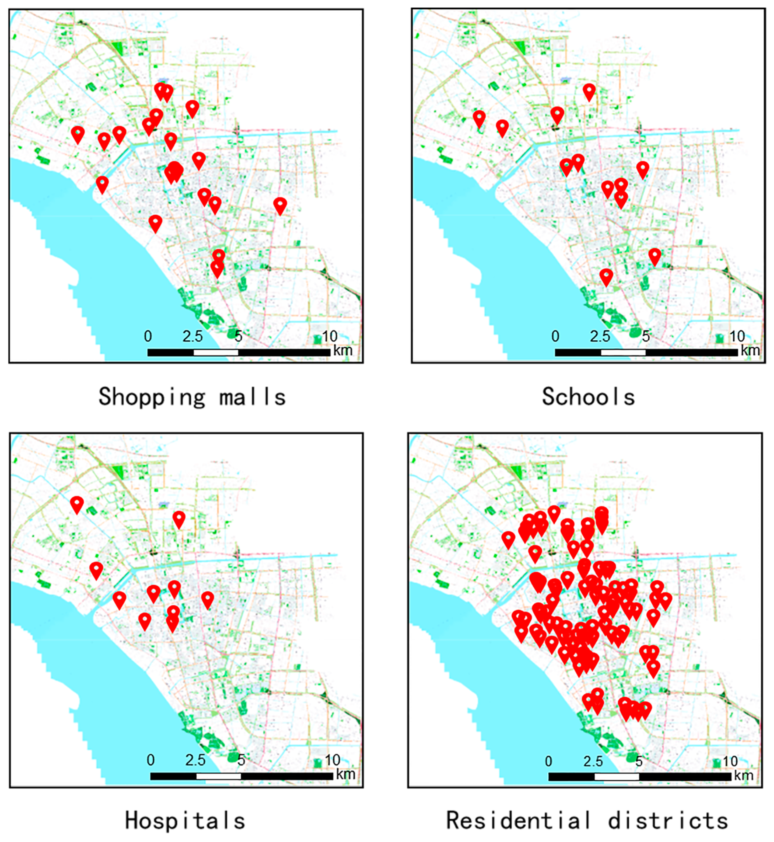
3.1.2. AOI Data

This paper used Nantong, China as the research area. AOI data were obtained using Amap API via web crawler technology. We selected several different types of AOIs for the experimental data, including shopping malls, schools, hospitals, and residential districts (Figure 8). The details of each type of AOI are shown in

Table 2. The samples of each type of AOI.

Type	AOI
Shopping mall	20 shopping malls (e.g., Wuzhou Square)
School	12 colleges and vocational schools (e.g., Nantong University)
Hospital	10 hospitals (e.g., the affiliated hospital of Nantong University)
Residential district	116 residential districts (e.g., Demin Garden community)

. In this experiment, 50 samples in the Chongchuan District were selected as the training set and 108 samples in the Gangzha District were collected as the validation set.

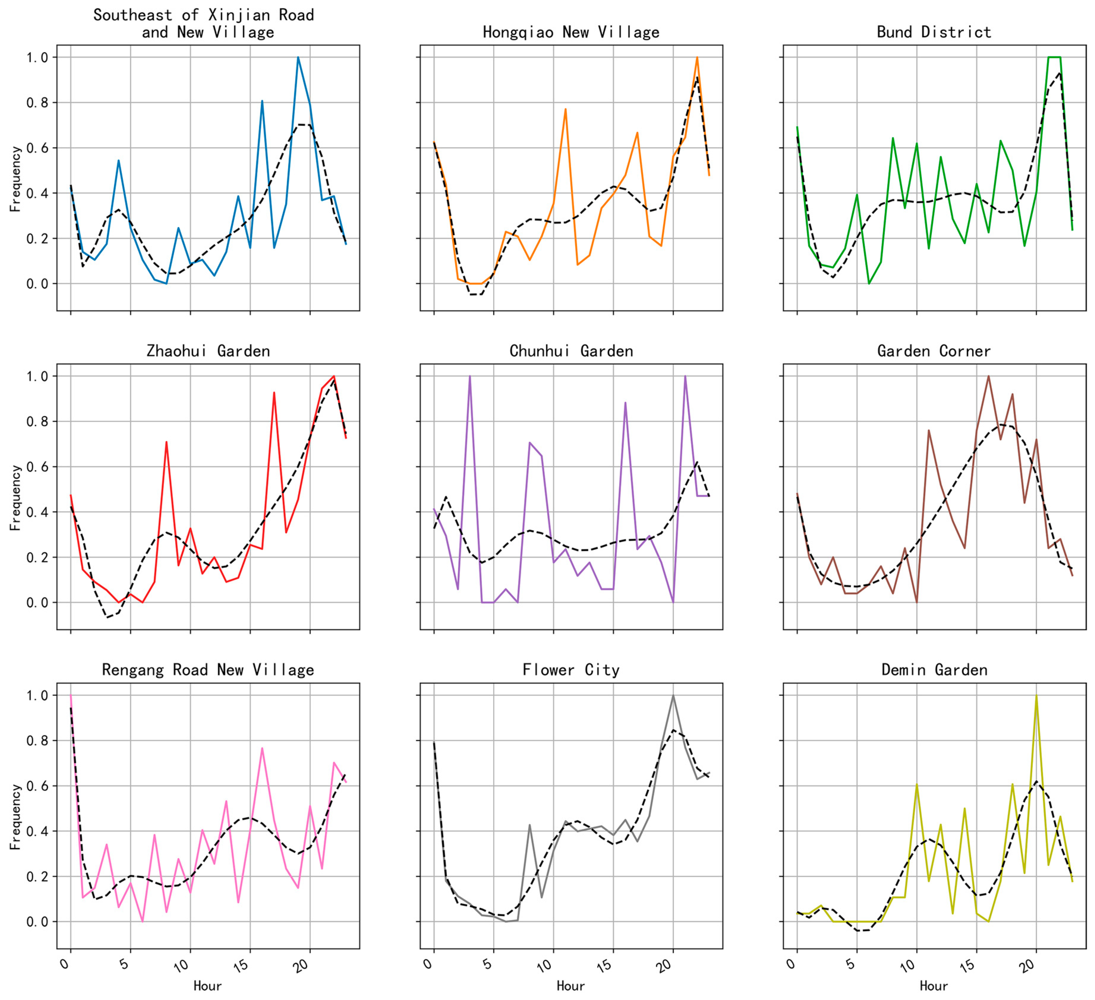
3.2. Training Results of the SHDSs

Fifty AOI samples were used to construct six types of HDSs. Taking the total drop-offs of the HDS of residential districts as an example, 78% of residential districts were found to have peaks at 10 a.m. and 8 p.m., and there were some abnormal fluctuations in different HDSs, but the overall trend was the same, as shown in Figure 9. Other types of AOIs, such as shopping malls, schools, and hospitals, also have a similar regularity and abnormal fluctuations.

The SHDS of the corresponding spectrum sequence of each type of AOI was calculated, and sampling at interval points was performed. In this experiment, we set m equal to 1, meaning sampling at every other point was performed, followed by interpolation. After standardizing the results of the SHDSs, the standard spectrum of each type was obtained, and these are shown in Figure 10. The Pearson correlation coefficient was used to calculate the correlation of the six SHDSs of each type of AOI. The average correlations of schools, communities, hospitals, and shopping malls were found to be 0.907, 0.743, 0.940, and 0.918. Each SHDS of each type of AOI shows the same trend. Taking the hospital as an example, there is a peak at 9 a.m. and 3 p.m. Taking the SHDS of the DP (Drop-off points) type as an example, as shown in Figure 11, the spectrum trends of different AOIs are different: there are two peaks in the hospital and three peaks in the school; the SHDS of the residential district shows an upward trend, while the other spectrum has a downward trend after rising.

3.3. Social Functional Identification of AOIs

Appropriate similarity indicators are the key to the matching method, which can improve the accuracy of identification. Thus, this article compares three different similarity indicators.

3.3.1. Cosine Similarity

The smaller the angle between the two vectors, the more similar the two vectors are. The cosine similarity abides by this theoretical idea. It measures the similarity between vectors by calculating the cosine of the angle between the two vectors. The derivation formula of cosine similarity is shown as

$$Similarity\left(X,Y\right)=\frac{X·Y}{\Vert X\Vert \times \Vert Y\Vert }=\frac{{{\displaystyle \sum }}_{i=1}^n\left(x_i\times y_i\right)}{\sqrt{{{\displaystyle \sum }}_{i=1}^n{\left(x_i\right)}^2}\times \sqrt{{{\displaystyle \sum }}_{i=1}^n{\left(y_i\right)}^2}}$$

(6)

where $X$ and $Y$ denote the vectors to be calculated. $x_i$ denotes the $i$th element in $X$, and $y_i$ denotes the $i$th element in $Y$, as shown in Figure 12.

3.3.2. Pearson Correlation Coefficient

Pearson correlation, also known as product difference correlation (or product–moment correlation), is a method of calculating correlations which was proposed by British statistician Pearson in the 20th century. The larger the absolute value of the correlation coefficient, the stronger the correlation. The closer the correlation coefficient is to −1 or 1, the stronger the correlation degree is, and the closer to 0, the weaker it is. In general, the correlation strength of variables can be determined using the following ranges: 0.8–1.0, extremely strong correlation; 0.6–0.8, strong correlation; 0.4–0.6, moderate correlation; 0.2–0.4, weak correlation; 0.0–0.2, extremely weak correlation or no correlation.

$$Similarity\left(X,Y\right)={\mathsf{\rho }}_{X,Y}=\frac{cov\left(X,Y\right)}{{\sigma }_X{\sigma }_Y}=\frac{E\left(\left(X-{\mu }_X\right)\left(Y-{\mu }_Y\right)\right)}{{\sigma }_X{\sigma }_Y}=\frac{E\left(XY\right)-E\left(X\right)E\left(Y\right)}{\sqrt{E\left(X^2\right)-E^2\left(X\right)}\sqrt{E\left(Y^2\right)-E^2\left(Y\right)}}$$

(7)

where $E$ denotes the mathematical expectation, $cov$ denotes the covariance, and $N$ denotes the number of variables.

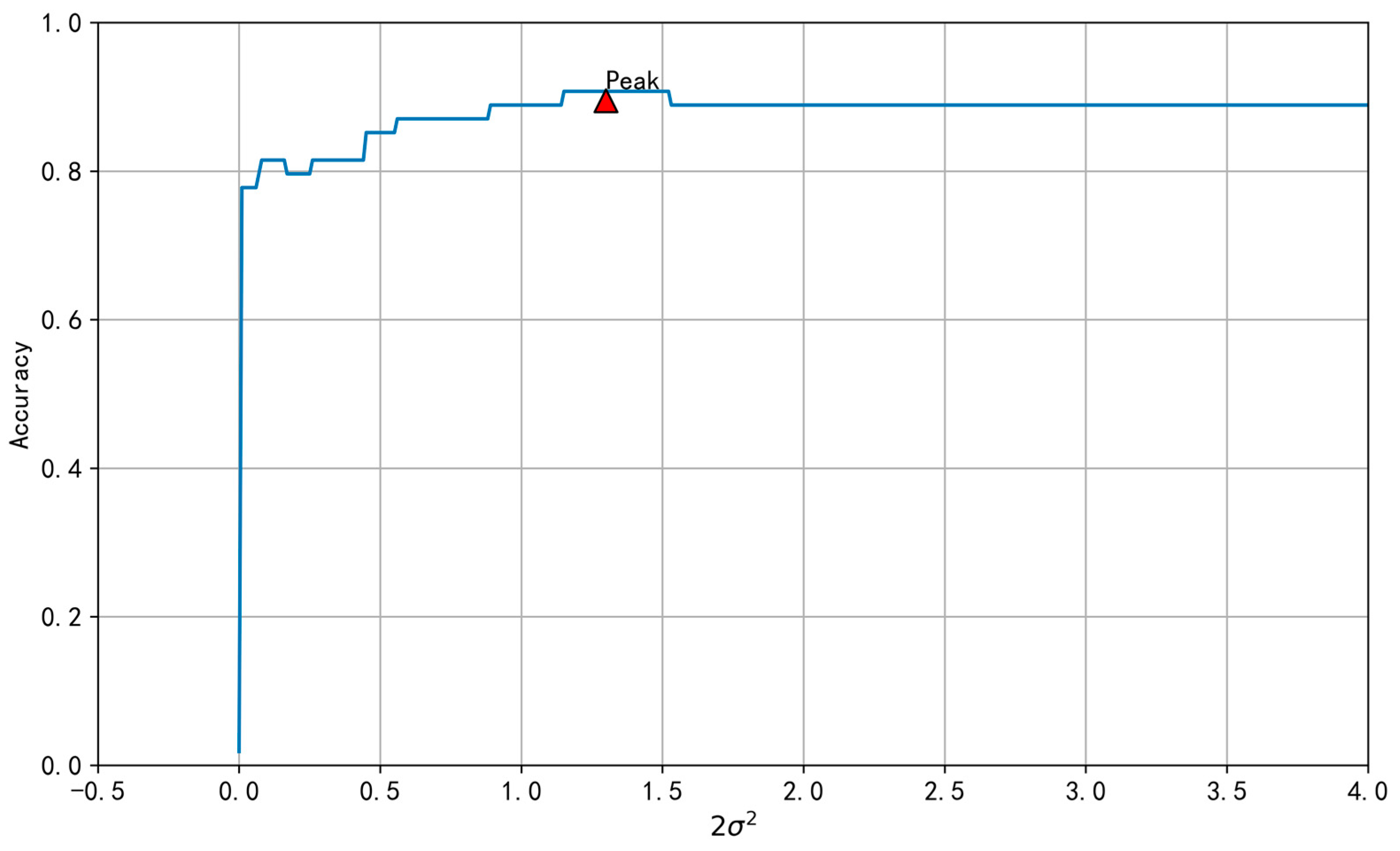
3.3.3. Gaussian Kernel Function

The Gaussian kernel function is defined as a monotone function of Euclidean distance between $X$ and $\mathrm{Y}$ in space, and is an effective method used to calculate the similarity between vectors. The farther the distance, the higher the difference between individuals. Hence, this paper takes the Gaussian kernel function as the similarity indicator, such as in the following formula, i.e.,

$$Similarity\left(X,Y\right)=e^{(-\frac{{\Vert X-Y\Vert }^2}{2{\sigma }^2})}$$

(8)

where $e$ denotes the natural logarithm and $\sigma$ denotes the standard deviation.

Three similarity indicators were used to validate the SHDSs of four types of AOIs, so the value range of the results are different. The self-correlation values were then normalized for comparison, as shown in Figure 13, Figure 14 and Figure 15. The heat map was used to reflect the similarity of different AOIs’ SHDSs. The darker the color, the higher the similarity. The color of the main diagonal, whose values are 1, is the darkest, which shows that the correlation between the same type of HDS is 100%. ‘M’, ‘R’, ‘S’ and ‘H’ in the maps represent shopping malls, residential districts, schools, and hospitals, respectively.

In the DP heat map of the Pearson correlation coefficients, as shown in Figure 12, the correlation coefficient between the SHDS of the residential district and the mall is 0.36, displaying a weak correlation, while the correlation coefficient between the SHDS of the mall and the hospital is 0.87, showing an extremely strong correlation. Obviously, the self-correlation of the Pearson correlation coefficient is the highest among the three, so the matching accuracy based on it is significantly lower than the others. Also affected by the strong self-correlation, the matching result based on cosine similarity is not ideal, being only 85.19%. By adjusting the value of 2${\sigma }^2$ of the Gaussian kernel function, an appropriate parameter can be found to enhance the constraint degree of HDS mutual matching during identification. The weight selection and accuracy comparison are shown in Figure 16.

When 2${\sigma }^2$ is less than 1.15, the accuracy shows an upward trend. When 2${\sigma }^2$ is greater than or equal to 1.15 and less than or equal to 1.52, the accuracy reaches the peak value, which is 90.74%. When 2${\sigma }^2$ is higher than 1.52, the accuracy gradually declines and eventually converges to 88.88%, as shown in

Table 3. Accuracy of different similarity indexes.

Similarity Index	Accuracy of Model
Pearson correlation coefficient	83.33%
Cosine similarity	85.19%
Gaussian kernel function ($2{\mathsf{\sigma }}^2$ = 1.5)	90.74%

. Hence, we selected the Gaussian kernel function in which 2${\sigma }^2$ is 1.5 as the similarity indicator.

4. Discussion

Partial identification results of the AOIs obtained via the proposed method are shown in

Table 4. Comparison of the identification results.

Original AOI	Real Type	Prediction	Result
Huaqiang City	Residential district	Residential district	Correct
Hongming Moore Square	Mall	School	Error
Yiyuan Beicun South District	Residential district	Residential district	Correct
Yiyuan Beicun North District	Residential district	Residential district	Correct
Nantong Secondary Professional School	School	School	Correct
Vientiane City	Mall	Mall	Correct
Vanke Golden Mile Plaza	Mall	Mall	Correct
Vanke Golden Mile Blue Bay	Residential district	Residential district	Correct
Qinzao New Village	Residential district	Residential district	Correct
Yiju Beiyuan	Residential district	Residential district	Correct
Jinyue Bay	Residential district	Residential district	Correct
Shang Haicheng	Residential district	Residential district	Correct
Sixth People’s Hospital	Hospital	School	Error
Starry Washington	Residential district	Residential district	Correct

, where the experimental accuracy is 90.74%.

The main reasons for the incorrect cases are as follows:

• Mutual interference between different types of AOIs
  AOIs are in fact on different levels. For example, hospitals can be divided into several levels. The higher the level, the greater the influence. If there is a significant level difference between two adjacent AOIs, it may result in the unclear attribution of the surrounding trajectory data. For example, Nantong First People’s Hospital and Nantong First Middle School are adjacent, as shown in Figure 17, but the influence of the First People’s Hospital is much stronger than that of the First Middle School. Hence, most of the trajectory data near the school were allocated to the hospital, meaning that the spectral information was not typical. In this case, we can consider accumulating data for an extended period and extracting data with a small buffer area for big data analysis, which is one of the research plans for the future.
• AOIs are newly built or have an abnormal status
  Exploring the correlation between AOIs and travel behavior requires a series of data points. Some buildings or residential districts are newly built or may not be open to the public, as shown in Figure 18. Due to the low occupancy rate, the number of drop-off points is insufficient to support the analysis of the spectrum. The entrance of the individual AOIs may need to rebuilt, which could also result in an abnormal status.
• Impact of the spatial location
  Theoretically, the closer to the center of the city, the more prosperous, and the stronger the regularity. On the contrary, when close to the edge of the city, the regularity is weakened.

5. Conclusions

A top-down supervised classification method has been proposed in this article using dynamic taxi pick-up and drop-off points to identify the social functional types of AOIs, so as to support the identification of urban functional partitions. Firstly, taxi trajectory data were used to replace the evaluation index of human travel behavior, and the relationship between the social function of AOIs and travel behavior was established. There was a strong correlation between these two things, and SHDS was obtained through the AOI samples. Then, using multiple SHDS and KNN methods, automatic identification and monitoring of the social function of AOIs were implemented. Finally, the experimental accuracy, which was up to 90.74%, was verified by various methods. Due to the continuous collection of taxi GPS trajectory data in many cities, this solution will serve as an effective long-term solution. Meanwhile, if this method is combined with image interpretation and other identification methods, better results can be achieved. Compared with cities such as Shanghai or Guangzhou, Nantong has a smaller population in its main urban area, meaning Nantong is a small city and the types of AOIs are not rich enough. If the experiment is able to be carried out in a big city, it may achieve better results. Because most AOIs in China, such as buildings and residential districts, are enclosed by walls and are only accessible via one or more entrances, this method is more suitable for most cities in China rather than those in other countries with an open management mode.

References

- Hu, Y.; Gao, S.; Janowicz, K.; Yu, B.; Li, W.; Prasad, S. Extracting and understanding urban areas of interest using geotagged photos. Comput. Environ. Urban Syst. 2015, 54, 240–254. [Google Scholar] [CrossRef]
- Zhou, T.; Liu, X.; Qian, Z.; Chen, H.; Tao, F. Dynamic Update and Monitoring of AOI Entrance via Spatiotemporal Clustering of Drop-Off Points. Sustainability 2019, 11, 6870. [Google Scholar] [CrossRef] [Green Version]
- Du, Z.; Zhang, X.; Li, W.; Zhang, F.; Liu, R. A multi-modal transportation data-driven approach to identify urban functional zones: An exploration based on Hangzhou City, China. Trans. GIS 2019, 1–19. [Google Scholar] [CrossRef]
- Wang, J.; Lin, Y.; Glendinning, A.; Xu, Y. Land-use changes and land policies evolution in China’s urbanization processes. Land Use Policy 2018, 75, 375–387. [Google Scholar] [CrossRef]
- Zhang, C.; Sargent, I.; Pan, X.; Li, H.; Gardiner, A.; Hare, J.; Atkinson, P.M. An object-based convolutional neural network (OCNN) for urban land use classification. Remote Sens. Environ. 2018, 216, 57–70. [Google Scholar] [CrossRef] [Green Version]
- Huang, Q.; Huang, J.; Zhan, Y.; Cui, W.; Yuan, Y. Using landscape indicators and Analytic Hierarchy Process (AHP) to determine the optimum spatial scale of urban land use patterns in Wuhan, China. Earth Sci. Inform. 2018, 11, 567–578. [Google Scholar] [CrossRef]
- Simwanda, M.; Murayama, Y. Spatiotemporal patterns of urban land use change in the rapidly growing city of Lusaka, Zambia: Implications for sustainable urban development. Sustain. Cities Soc. 2018, 39, 262–274. [Google Scholar] [CrossRef]
- Gao, P.; Wang, J.; Zhang, H.; Li, Z. Boltzmann entropy-based unsupervised band selection for hyperspectral image classification. IEEE Geosci. Remote Sens. Lett. 2018, 16, 462–466. [Google Scholar] [CrossRef]
- Lei, C.; Zhang, A.; Qi, Q.; Su, H.; Wang, J. Spatial-temporal analysis of human dynamics on urban land use patterns using social media data by gender. ISPRS Int. J. Geo-Inf. 2018, 7, 358. [Google Scholar] [CrossRef] [Green Version]
- Huang, B.; Zhou, Y.; Li, Z.; Song, Y.; Cai, J.; Tu, W. Evaluating and characterizing urban vibrancy using spatial big data: Shanghai as a case study. Environ. Plan B Urban Anal. City Sci. 2019, 1–17. [Google Scholar] [CrossRef]
- Jin, C.; Nara, A.; Yang, J.A.; Tsou, M.H. Similarity measurement on human mobility data with spatially weighted structural similarity index (SpSSIM). Trans. GIS 2019, 1–19. [Google Scholar] [CrossRef]
- Zhou, T.; Shi, W.; Liu, X.; Tao, F.; Qian, Z.; Zhang, R. A Novel Approach for Online Car-Hailing Monitoring Using Spatiotemporal Big Data. IEEE Access 2019, 7, 128936–128947. [Google Scholar] [CrossRef]
- Bruwier, M.; Mustafa, A.; Aliaga, D.G.; Archambeau, P.; Erpicum, S.; Nishida, G.; Zhang, X.; Pirotton, M.; Teller, J.; Dewals, B. Influence of urban pattern on inundation flow in floodplains of lowland rivers. Sci. Total Environ. 2018, 622, 446–458. [Google Scholar] [CrossRef] [PubMed] [Green Version]
- Melgani, F.; Bruzzone, L. Classification of hyperspectral remote sensing images with support vector machines. IEEE Trans. Geosci. Remote Sens. 2004, 42, 1778–1790. [Google Scholar] [CrossRef] [Green Version]
- Yi, K.; Zeng, Y.; Wu, B. Mapping and evaluation the process, pattern and potential of urban growth in China. Appl. Geogr. 2016, 71, 44–55. [Google Scholar] [CrossRef]
- Yuan, Q.; Zhang, L.; Shen, H. Hyperspectral image denoising employing a spectral–spatial adaptive total variation model. IEEE Trans. Geosci. Remote Sens. 2012, 50, 3660–3677. [Google Scholar] [CrossRef]
- Pal, M.; Foody, G.M. Feature selection for classification of hyperspectral data by SVM. IEEE Trans. Geosci. Remote Sens. 2010, 48, 2297–2307. [Google Scholar] [CrossRef] [Green Version]
- Cheng, G.; Han, J. A survey on object detection in optical remote sensing images. ISPRS J. Photogramm. 2016, 117, 11–28. [Google Scholar] [CrossRef] [Green Version]
- Liu, B.; Xiong, H.; Papadimitriou, S.; Fu, Y.; Yao, Z. A General Geographical Probabilistic Factor Model for Point of Interest Recommendation. IEEE Trans. Knowl. Data Eng. 2015, 27, 1167–1179. [Google Scholar] [CrossRef]
- Yue, Y.; Zhuang, Y.; Yeh, A.G.; Xie, J.-Y.; Ma, C.-L.; Li, Q.-Q. Measurements of POI-based mixed use and their relationships with neighbourhood vibrancy. Int. J. Geogr. Inf. Sci. 2017, 31, 658–675. [Google Scholar] [CrossRef] [Green Version]
- Goodchild, M.F.; Li, L. Assuring the quality of volunteered geographic information. Spat. Stat. 2012, 1, 110–120. [Google Scholar] [CrossRef]
- Zhuo, L.; Shi, Q.; Zhang, C.; Li, Q.; Tao, H. Identifying Building Functions from the Spatiotemporal Population Density and the Interactions of People among Buildings. ISPRS Int. J. Geo-Inf. 2019, 8, 247. [Google Scholar] [CrossRef] [Green Version]
- Shen, J.; Liu, X.; Chen, M. Discovering spatial and temporal patterns from taxi-based Floating Car Data: A case study from Nanjing. GIsci. Remote Sens. 2017, 54, 617–638. [Google Scholar] [CrossRef]
- Lu, M.; Liang, J.; Wang, Z.; Yuan, X. Exploring OD patterns of interested region based on taxi trajectories. J. Vis. 2016, 19, 811–821. [Google Scholar] [CrossRef]
- Wang, M.; Mu, L. Spatial disparities of Uber accessibility: An exploratory analysis in Atlanta, USA. Comput. Environ. Urban Syst. 2018, 67, 169–175. [Google Scholar] [CrossRef]
- Jasny, B.R.; Stone, R. Prediction and its limits. Science 2017, 355, 468–469. [Google Scholar] [CrossRef] [PubMed] [Green Version]
- Kong, X.; Xia, F.; Fu, Z.; Yan, X.; Tolba, A.; Almakhadmeh, Z. TBI2Flow: Travel behavioral inertia based long-term taxi passenger flow prediction. World Wide Web 2019, 1–25. [Google Scholar] [CrossRef]
- Brockmann, D.; Hufnagel, L.; Geisel, T. The scaling laws of human travel. Nature 2006, 439, 462. [Google Scholar] [CrossRef]
- Gonzalez, M.C.; Hidalgo, C.A.; Barabasi, A.-L. Understanding individual human mobility patterns. Nature 2008, 453, 779. [Google Scholar] [CrossRef]
- Liang, X.; Zheng, X.; Lv, W.; Zhu, T.; Xu, K. The scaling of human mobility by taxis is exponential. Phys. A 2012, 391, 2135–2144. [Google Scholar] [CrossRef] [Green Version]
- Tobler, W.R. A computer movie simulating urban growth in the Detroit region. Econ. Geogr. 1970, 46, 234–240. [Google Scholar] [CrossRef]
- Gao, Y.; Liu, J.; Xu, Y.; Mu, L.; Liu, Y. A Spatiotemporal Constraint Non-Negative Matrix Factorization Model to Discover Intra-Urban Mobility Patterns from Taxi Trips. Sustainability 2019, 11, 4214. [Google Scholar] [CrossRef] [Green Version]
- Demissie, M.G.; Phithakkitnukoon, S.; Kattan, L.; Farhan, A. Understanding Human Mobility Patterns in a Developing Country Using Mobile Phone Data. Data Sci. J. 2019, 18, 1–13. [Google Scholar] [CrossRef] [Green Version]
- Huang, J.; Liu, X.; Zhao, P.; Zhang, J.; Kwan, M.-P. Interactions between Bus, Metro, and Taxi Use before and after the Chinese Spring Festival. ISPRS Int. J. Geo-Inf. 2019, 8, 445. [Google Scholar] [CrossRef] [Green Version]
- Jiang, S.; Guan, W.; He, Z.; Yang, L. Measuring Taxi Accessibility Using Grid-Based Method with Trajectory Data. Sustainability 2018, 10, 3187. [Google Scholar] [CrossRef] [Green Version]
- Pan, G.; Qi, G.; Wu, Z.; Zhang, D.; Li, S. Land-use classification using taxi GPS traces. IEEE Trans. Intell. Transp. Syst. 2012, 14, 113–123. [Google Scholar] [CrossRef]
- Ord, J.K.; Getis, A. Local spatial autocorrelation statistics: Distributional issues and an application. Geogr. Anal. 1995, 27, 286–306. [Google Scholar] [CrossRef]
- Ester, M.; Kriegel, H.-P.; Sander, J.; Xu, X. A density-based algorithm for discovering clusters in large spatial databases with noise. In Proceedings of the Second International Conference on Knowledge Discovery and Data Mining, Portland, OR, USA, 2–4 August 1996; pp. 226–231. [Google Scholar]
- Zheng, L.; Xia, D.; Zhao, X.; Tan, L.; Li, H.; Chen, L.; Liu, W. Spatial–temporal travel pattern mining using massive taxi trajectory data. Phys. A 2018, 501, 24–41. [Google Scholar] [CrossRef]
- Hartigan, J.A.; Wong, M.A. Algorithm AS 136: A k-means clustering algorithm. J. R. Stat. Soc. Ser. C (Appl. Stat.) 1979, 28, 100–108. [Google Scholar] [CrossRef]
- Park, H.-S.; Jun, C.-H. A simple and fast algorithm for K-medoids clustering. Expert Syst. Appl. 2009, 36, 3336–3341. [Google Scholar] [CrossRef]
- Rodriguez, A.; Laio, A. Clustering by fast search and find of density peaks. Science 2014, 344, 1492–1496. [Google Scholar] [CrossRef] [PubMed] [Green Version]
- Goodman, A.; Cheshire, J. Inequalities in the London bicycle sharing system revisited: Impacts of extending the scheme to poorer areas but then doubling prices. J. Transp. Geogr. 2014, 41, 272–279. [Google Scholar] [CrossRef] [Green Version]
- Lovelace, R.; Goodman, A.; Aldred, R.; Berkoff, N.; Abbas, A.; Woodcock, J. The Propensity to Cycle Tool: An open source online system for sustainable transport planning. J. Transp. Land Use 2016, 10, 505–528. [Google Scholar] [CrossRef] [Green Version]
- Longley, P.A.; Adnan, M. Geo-temporal Twitter demographics. Int. J. Geogr. Inf. Sci. 2015, 30, 369–389. [Google Scholar] [CrossRef]
- Kempinska, K.; Longley, P.; Shawe-Taylor, J. Interactional regions in cities: Making sense of flows across networked systems. Int. J. Geogr. Inf. Sci. 2018, 32, 1348–1367. [Google Scholar] [CrossRef] [Green Version]
- Batty, M. Artificial intelligence and smart cities. Environ. Plan. B 2018, 45, 3–6. [Google Scholar] [CrossRef]