Prototyping of Environmental Kit for Georeferenced Transient Outdoor Comfort Assessment


1
Chair of Building Technology and Climate Responsive Design, Technical University of Munich, 80333 Munich, Germany
2
Chair of Architecture Informatics, Technical University of Munich, 80333 Munich, Germany
*
Authors to whom correspondence should be addressed.
ISPRS Int. J. Geo-Inf. 2019, 8(2), 76; https://doi.org/10.3390/ijgi8020076
Submission received: 30 November 2018
/
Revised: 13 January 2019
/
Accepted: 27 January 2019
/
Published: 5 February 2019
(This article belongs to the Special Issue Human-Centric Data Science for Urban Studies)
Abstract
:Environmental data acquisition tools are broadly used for climate monitoring and urban comfort assessment followed by data mining and sensing techniques for putting into evidence the relationship between environmental qualities of urban spaces and human well-being. Within this context, an environmental toolkit is a fundamental tool to evaluate transient outdoor comfort. This study explains the prototyping and validation of a mobile environmental sensor kit. The results show the prototype has reasonable accuracy despite its affordability with respect to industrial sensors.
1. Introduction
The extreme impacts of human activities are global warming and climate change, which pose countless threats to civilization [1]. Cities are particularly susceptible to the impacts of climate change due to their rapid expansion and dense population. They tend to experience higher temperatures with respect to their surroundings, an effect known as the urban heat island (UHI), indicating that their microclimates will be exposed to harsher environmental fluctuations compared to rural areas. The severity of UHI over time depends on climate and urban characteristics and context [2,3]. One of the climate change scenarios implies that the average annual temperature will rise by 1–5 °C after 2080 [4]. Furthermore, urban microclimates directly affect the quality of life in cities. As pedestrians are in constant interaction with the built environment, achieving outdoor thermal comfort can encourage the use of public spaces and sustainable means of transportation [5,6]. Some comprehensive environmental assessment techniques can be used to gather data and inform urban planning scenarios [7], and the improvements can reflect on local businesses and tourism, ensuring health, well-being, economy, and biodiversity of the cities.
Regarding human thermal comfort, it is essential to understand the causes of discomfort in urban public spaces in order to prefigure adaptation measures for societies to a new climatic context [8]. The past decade has seen an enthusiasm for planning cities for health, which had mostly been forgotten since the urban sanitarian movement in the mid-nineteenth century [9]. Discomfort is caused by inequality in heat exchange between the human body and its surroundings. In this regard, it is crucial to link microclimatic conditions to human physiology. The heat exchange mechanism considers the addition of heat (by metabolism and absorbed radiation) opposite to the loss of heat (by convection, evaporation, and emitted radiation) [10,11]. Prolonged heat stress or cold stress may force a thermoregulatory failure and lead to health issues like hyperthermia (elevated body temperature) or hypothermia (reduced body temperature). The consequences can vary from fatigue and nausea to permanent disabilities and death [12].
Therefore, every source of data regarding environmental conditions in cities is crucial for the analysis and observation of comfort and well-being variations and their consequences. The current analysis and simulation methods, such as global integrated surface dataset (ISD) along with geographic information system (GIS), computer-aided design (CAD), computer-aided engineering (CAE), and computational fluid dynamics (CFD), help urban planners to predict and comprehend their climatic conditions. Many complex problems like the interactions between urban street canyons [13] and UHI are estimated with computational simulations [14,15]. Occasionally, uninterrupted data acquisition tools like mobile weather stations are used to retrieve environmental data at a microclimate level. Such datasets can influence analytical decisions while planning, reshaping, and reactivating urban contexts. It can also be beneficial for the elaboration of climatic patterns and for environmental predictions with higher resolution.
Nowadays, the use of open-source technologies by professionals and technology enthusiasts is growing due to their common access to the Arduino and Raspberry-Pi prototyping platforms with evolutionary source codes and schematics. Many researchers use this platform to build data loggers for the specific datasets that interest their studies. Fuentes et al. [16] developed a new data logger using the Arduino open-source electronic platform to solve the current problem of monitoring photovoltaic (PV) systems at low cost, especially in remote areas or regions in developing countries. Likewise, Ali et al. [17] proposed the Open Source Building Science Sensors (OSBSS) Project, which was created to design and develop a suite of inexpensive, open-source devices based on the Arduino platform to measure and record long-term indoor environment and to build operational data. By the same token, Baker [18] incorporated real-time environmental monitoring methodologies using low-power and low-cost computing platforms. This study also considered it sensible to use available open-source platforms to acquire and visualize environmental data while focusing on outdoor thermal comfort with geo-referencing techniques.
Environmental data loggers are widely used assets for climate monitoring indoors; however, there is a lack of applications for climate monitoring outdoors. At the same time, branded industrial data loggers are often expensive and are not easily accessible for users. In this context, this research investigates methods to promote more constant acquisition and widely available environmental datasets using Arduino-based sensors. The prospective application of the development follows two main objectives. The first is to help decision-makers and urban planners toward transient outdoor comfort assessments to capture correlations between microclimate and the built environment. The second objective follows the concept of open-source environmental datasets, aiming for adequate accuracy with low-cost sensors. Moreover, the development can be beneficial for architects, environmental scientists, civil engineers, urban planners, and policy-makers to make data-integrated design decisions.
The major contribution of this paper is to demonstrate the prototyping process of an environmental kit that can sense conditions with a portable, affordable device. We present the objectives and the prototyping methodology, including a description of all components. In the next section, we describe the data acquisition process and the validation. The following section presents the method to model the acquired georeferenced data for the primary application. We finish by presenting our conclusions and discussing future work.
2. Objectives and Process
This study reports on the development of an outdoor comfort assessment tool based on Arduino [19] prototyping with the available environmental sensors. The process begins with the physical connections of the sensors to the microcontroller unit and software coding. In the following phase, the developed tool is tested parallel to its industrialized counterpart. To test the transient application of the device, outdoor thermal comfort maps are demonstrated with the measured data by walking through urban spaces. The final phase concludes with a discussion on short-term and long-term improvements to the device.
The programming platform is the Arduino integrated development environment (IDE), which uses C and C++ languages. The data is compared with the measurements from branded environmental data loggers. Subsequently, the tool is used to collect georeferenced data in Munich, Germany. For the evaluation, the data is mapped using Grasshopper3D to visualize distinctive microclimates and pedestrian thermal comfort using the universal thermal climate index (UTCI) [20,21,22].
The incentive is to equip architects and urban planners with a tool that can be easily assembled and modified according to the user’s needs. In future, multiple hubs can be established within urban communities to retrieve sensible data. The device may also be expended as a weather station.
3. Prototyping Methodology
3.1. Modeling and Sensors Overview
The intended data acquisition tool (Weather-Gear) requires both hardware and software development. The hardware segment consists of a collection of environmental sensors connected to the microcontroller board. The microcontroller receives power from a 9 volt (V) direct current (DC) source. The microcontroller’s embedded voltage regulator can supply 3.3 V, 5 V, and the source voltage (input voltage, 9 V) for the sensors. The microcontroller is programmed by a computer through the universal serial bus (USB). The sensor data can be logged into an SD card. The same data can be viewed and saved on the internet through the Wi-Fi module or the IDE terminal via USB interface. An outline of the model is illustrated in Figure 1.
The environmental sensors include air temperature, relative humidity, globe temperature, wind speed, and global solar radiation. A GPS module is used to attain real-world coordinates. The SD card sloth and real-time clock (RTC) are connected to the microcontroller for data logging. The microcontroller’s built-in USB port is used for primary communication. A Wi-Fi module is connected for effortless user-to-device interaction. The main challenges for the hardware are accuracy and reaction time of the sensors and precision of the RTC. The secondary challenge is the enhancement of functionality relevant to the user’s demand. For this purpose, particulate matter and noise pollution sensors are added. Additional data will be extracted from GPS, such as mobility speed, number of satellites in view, and altitude. The implemented components and sensors over the prototyping process are listed in Table 1.
The software side of the project includes microcontroller programming with the Arduino IDE. Thereafter, real-time commands can be sent to the microcontroller through IDE terminal, web browsers, and smartphone applications.
3.2. Prototype Development
Our primary objective was to gather relevant environmental data. The secondary objective was to communicate the data to a smartphone for a better user experience. Therefore, the development started with two mini projects from public libraries to present the opening idea. The first stage included a simple display of data on the LCD, and the second stage communicated the data using Wi-Fi.
3.2.1. Displaying Sensor Readings on LCD
At this stage, a temperature–humidity sensor (DHT11), a liquid crystal display (LCD) (1602) screen, and a potentiometer (10 kΩ) are attached to the Arduino microcontroller unit (MCU). The data obtained include relative humidity, the air temperature in degree Celsius, the air temperature in Fahrenheit, and the heat index.
3.2.2. Displaying Sensor Readings on Smartphone
In this step, the DHT11 sensor is attached to an ESP8266 Huzzah board as the MCU with a built-in Wi-Fi sensor. The data is successfully monitored through a smartphone. For user interface, Internet of things (IoT) application “Blynk” is utilized. The data can be viewed in real time and also logged in for future use through the application. These steps show the fundamental concept of the project. Henceforth, the focus is on applying this concept with relevant sensors to acquire adequate data collection for outdoor comfort analysis.
3.2.3. Expansion of the Environmental Parameters
After a successful display of the concept, the MCU is connected with a different set of sensor modules. The prototype evolves step-by-step with the attachment of each component. The process starts with separate tests for each sensor, challenging for relevant outputs owing to connections with the MCU and the available IDE codes. After passing the first test, each sensor and the related code is added in the program. The results are monitored, and the code is further modified to focus on important data and to filter out unnecessary yields. This process is repeated in a loop format until the results fulfill the project’s scope. The prototyping process is further elaborated in Figure 2.
3.2.4. Breadboard Connections and Schematics
The Arduino Mega was specifically selected because of the wide collection of pins and compatibility with most of the sensors. The selected data logger is mounted on top of the MCU. For its I²C connection, the serial data (SDA) and serial clock (SCL) pins from the MCU are connected to analog pins A4 and A5 of the data logger shield. The IDE code and SD libraries are also slightly modified. The I²C connection and code modifications are specific to the project’s data logger and are skipped in the latest versions of the shield. The attached RTC is powered by a CR1220 coin cell to avoid redundant programming as the RTC resets the time when power is not available. The DS18B20 temperature sensor is attached to the MCU through digital communication. A 4.7 kΩ pull-up resistor is connected in parallel between the data and VDD lines. As a one-wire sensor, it has a unique 64-bit serial number; therefore, a vast number of one-wire sensors can share the same bus. The code includes a sensor temperature request in the loop and calls the sensor by index; 0 refers to the first sensor on the bus. The SHT20 humidity and temperature sensor is controlled by the I²C protocol. The sensor is initiated in the void setup, and its specific library is included at the beginning of the code. The TSL2561 luminosity digital sensor is a 3 V logic module, but due to its internal 3.6 V voltage regulator, it can be connected directly to 5 V of the Arduino board. Therefore, there is no logic level issue with I²C connections. The I²C lines SDA and SCL are joined parallel to SHT20 sensor’s data and clock bus. The address change pin (ADDR) can be used to avoid I²C address conflict, but it remains idle in our circuit. Similarly, the interrupt (INT) output pin is also disconnected. This pin is used for configuration of the sensor with a change in the level of light.
The pinouts for TCS34725 is exactly the same as that of TSL2561. The only addition to the layout is the LED pin that is connected to GND to turn off the built-in LED. This LED projects light (4150 K neutral) on an object for color sensing.
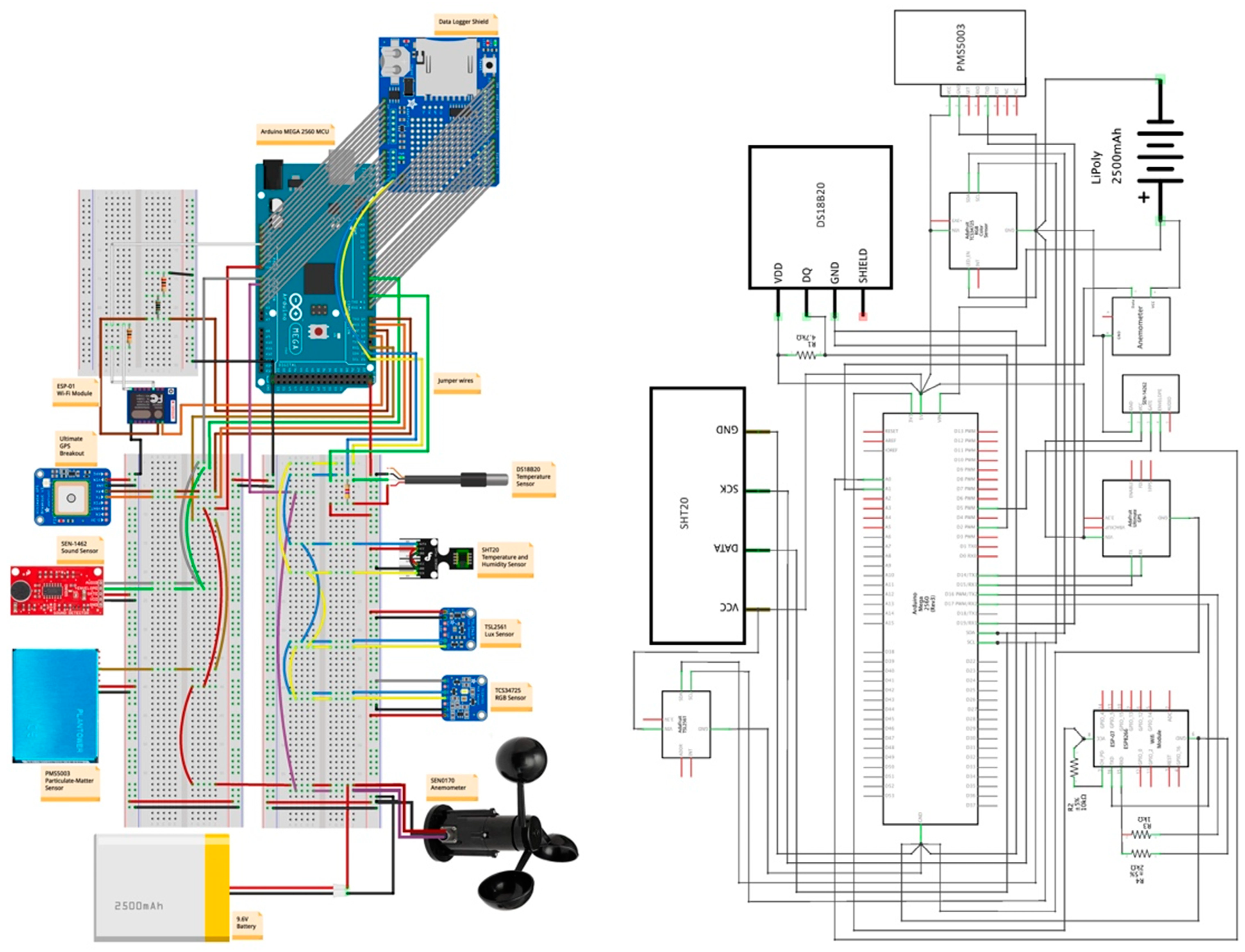
The SEN0170 anemometer’s VDD line is connected to an external 9.6 V DC supply, and the GND is connected to Arduino GND. The same battery powers the MCU when detached from the USB supply source. The data line is attached to an analog pin of the MCU to transmit sensor readings. The PMS5003 particulate matter sensor is attached to the MCU’s universal asynchronous receiver/transmitter (UART); transmitter line (TX) to the receiver (RX1) of the MCU. The rest of the sensor pins are not used in our project. The sound detector (SEN-1462) is also powered from the MCU. The sensor’s gate pin is attached to the MCU for a digital signal, while the envelope transmits analog data. The audio pin remains unused in our project. The GPS module is powered by the MCU’s 5 V supply. The mode of communication is UART by attaching a transmitter line of the GPS to the receiver of MCU and vice versa. The ESP-0 Wi-Fi module connection includes several steps to flush the old firmware and install new firmware through an FTDI serial adaptor. In the absence of an adaptor, a voltage divider is used as the Wi-Fi module is a 3 V device. The module demands a supply current of 300 mA, while the maximum current supplied by the Arduino at 3 V rail is 200 mA. Therefore, an external supply must be used for the ESP-01 module. A voltage divider is used between the RX pin of the ESP and the TX pin of the Arduino as the 5 V logic can fry the Wi-Fi module. The connections are further explained through breadboard diagram and schematics diagram in Figure 3.
3.2.5. Portable Case
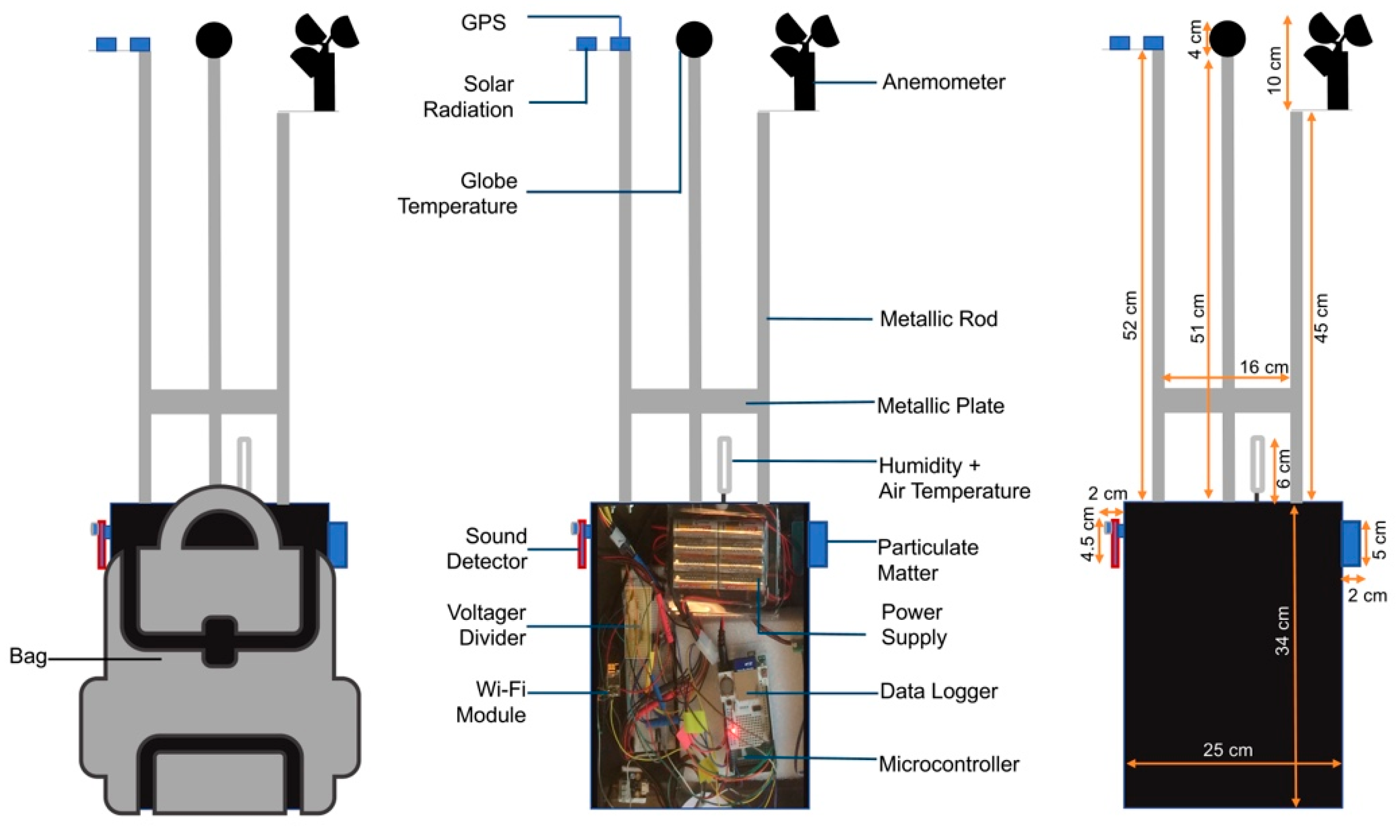
An external shell was made by stacking two rectangular trays and fixing them with screws to protect the electronic circuits. The Arduino MCU, the battery, the data logger, the Wi-Fi module, and the wires are enclosed within this plastic-box. The GPS, RGB (red, green, blue), illuminance, wind speed, and globe temperature sensors are elevated from the box by hollow metallic rods (approx. 50 cm from the box). There is a gap (approx. 8 cm) between the rods to avoid shadows of one sensor on the other. The air temperature plus humidity probe is fastened at the top edge of the casing for data procurement at human shoulder level. The particulate matter sensor and the sound detector are engraved on the top-right and top-left side of the box, respectively. Metallic plates are used to fix the rods on the exterior body. This rectangular package can be placed inside a bag to be carried conveniently by the user. The globe temperature sensor (DS18B20) is enclosed in a blackened table tennis ball. The positioning of the components and the dimensions of the prototype is further explained in Figure 4.
4. Data Acquisition and Handling
The sampling of an observed physical phenomena and the conversion of the samples into compatible numerical values for computer analysis is called data acquisition. The real-world conditions are measured with fluctuations in electrical signals of certain material in reference to those conditions. By nature, these signals are analog, which is amplified and converted into digital signals. The digital signals are packets of 0 s and 1 s, which are converted into the decimal system by an interpreter. The processed data is stored in the R/W memory of the computer. A simple data acquisition system (DAS) is outlined in Figure 5.
With the abovementioned procedure, the developed prototype receives and processes the environmental data sets. The measurements are monitored through IDE terminal and saved in the SD card for future assessment. The connected sensors are called one after the other in the following order according to the prototype’s programming code:
- Globe temperature () sensor
- Air temperature (), and relative humidity () sensor
- Anemometer
- RGB and illuminance sensors
- GPS
- Particulate matter () sensor
- Sound detector
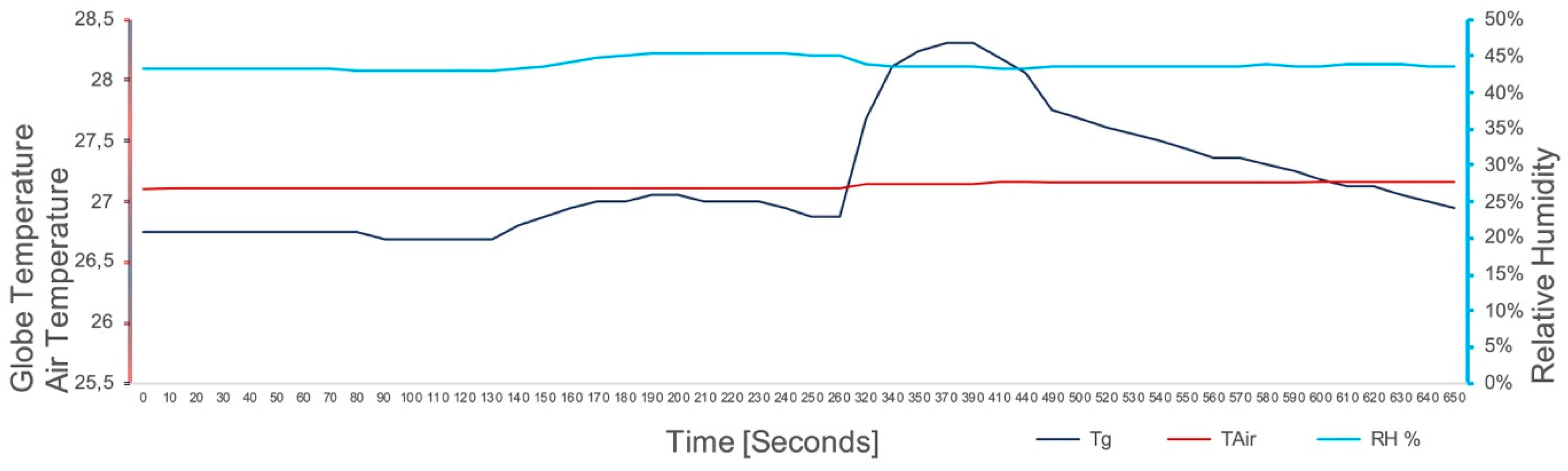
The data received from the , , and sensors are converted and saved in the international system of units (SI). Although additional coding can be made for unit conversion or calculating heat index, our data remains confined to air temperature, globe temperature, and relative humidity from these two sensors (Figure 6).
4.1. Wind Speed Reading from Voltage
The anemometer simultaneously compares output voltage signal (0–5 V) to determine the wind speed. The sensor calculates these values from output voltage with the following equation:
4.2. Mean Radiant Temperature
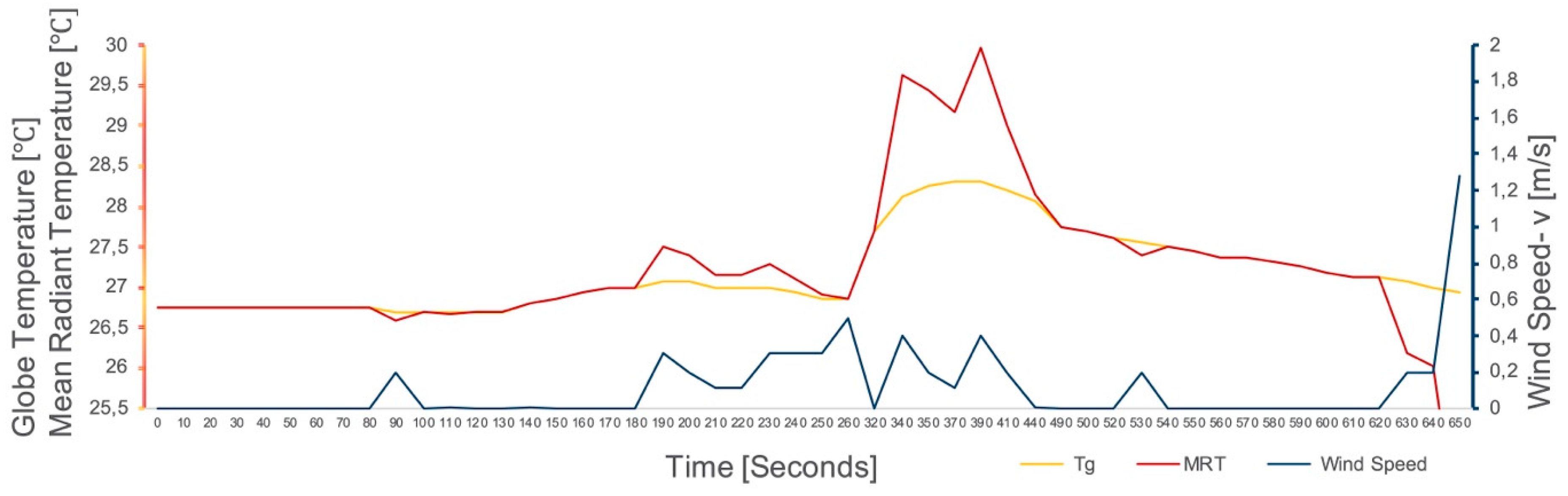
The average temperature of all surfaces that surround a particular point with which it will exchange thermal radiation is called the mean radiant temperature (MRT). The surroundings may include solar radiation and sky temperature in outdoor situations [23]. The MRT can be measured with a globe temperature, air temperature, and wind speed with the following formula [24]:
where refers to the globe temperature, refers to the air temperature, refers to the air velocity, ε refers to the emissivity of the globe, and refers to the globe diameter.
A comparison of the prototype parameters (globe temperature and wind speed) and the calculated MRT is shown in Figure 7.
4.3. Solar Radiation
The radiant (electromagnetic) energy received from the sun is known as solar radiation. There are three main bands on the solar spectrum distributed at different wavelengths, i.e., ultraviolet (100 nm to 400 nm), visible (400 nm to 700 nm), and infrared (700 nm to 1 mm). The visible light is also referred to as photosynthetically active radiation (PAR). The infrared radiation (IR) covers most of the solar spectrum, but the energy of the solar radiation is distributed. The division includes up to 49.4% in IR range, 42.3% in the PAR range, and about 8% in the UV range [25].
The irradiance of the sun dropping on the earth’s atmosphere varies up to 6.6% throughout the year due to changes in the distance between them. The mean distance is about 149,597,890 km (1 AU). The irradiance of the sun on the outer atmosphere at the mean distance is called the solar constant. The accepted values for the solar constant range according to the National Aeronautics and Space Administration (NASA) is 1353 ± 21 , while the World Meteorological Organization (WMO) recommends 1367 . The solar constant is the sum of irradiances at different wavelengths distributed over the solar spectrum.
The range of the solar spectrum is largely between 200 and 2500 nm in space, and it divides into numerous segments at the earth’s surface. The terrestrial spectra consist of direct radiation, diffuse radiation, and reflected radiation (dependent upon a location’s albedo), while the sum of direct and diffuse radiation is known as global radiation.
The radiation spectrum experiences frequent alterations after passing through the atmosphere. Clouds can block most of the direct solar radiation. Similarly, drifts in the ozone layer and seasonal deviations also have significant effects on the ultraviolet segment of the spectrum. These modifications are caused due to absorption and scattering by oxygen, nitrogen, carbon dioxide, and water molecules in the atmosphere. The terrestrial irradiance in clear sky conditions may reduce to ca. 1050 direct radiation and ca. 1120 global radiation from 1367 in space.
The extraterrestrial spectrum is called “Air Mass 0” (AM0) as it does not pass through any air mass. When the sun is at its zenith and direct radiation passes through the atmosphere completely, it is known as “Air Mass 1 Direct” (AM1D) radiation. The standards suggest sea level as a reference site. Similarly, “Air Mass 1 Global” (AM1G) refers to the global radiation with overhead sun. Three spectra have been published by the American Society for Testing and Materials (ASTM)—AM0, AM1.5 Direct, and AM1.5 Global for tilted surfaces—“at 37° angles for the USA”. The collimation of direct solar radiation occurs at circa 0.53°, whereas the diffuse radiation is received from ground reflections, atmospheric scatter, and diffusion through the sky. The global radiation is broadly unvarying. The aerosol causes a high distribution of solar radiation by scattering, causing a ring at the rim of the solar disk called the solar aureole. The direct beam in addition to the solar aureole is known as circumsolar radiation [26].
4.3.1. Illuminance Conversion to Irradiation
The detection and measurement of electromagnetic radiation are known as radiometry, and the subset of radiometry for a typical human eye response (visible spectrum) is known as photometry. To generalize, irradiance is the radiometric measurements of the solar spectrum that is observed as power per unit area (Watt/meter2), while the photometric spectrum is measured in lux (lumen/meter2). The amount of radiant flux incident on a known surface area is called irradiance, and the total visible energy emitted by a light source is known as luminous flux.
The photopic spectral luminous efficiency curve, by the commission of illumination (CIE), gives the spectral response of the human eye to various wavelengths of light and is used to convert between radiometric and photometric units. The wavelength at which the human eye is most sensitive is known as the wavelength of unity (concerning scotopic and photopic curves) with a value of 555 nm. The following reference is used as a scaling factor for the unit conversion:
1 watt (555 nm) = 683 lumen
Radiometric power is converted into luminous flux using the following integral equation [27]:
where Φv = flux (Lumen), Pe = power (Watt), V = photopic response function of the human eye, K = constant (683 lm/W for photopic), and λ = wavelength (380 nm to 780 nm).
There is a nonstandard estimate value for conversion of illuminance to irradiance in the visible spectrum. The value (0.0079 W/m2 per lux) can be used to find approximate irradiance using photometric sensors. For example, illuminance of 45,000 lux calculated by an illuminance sensor can be converted into irradiance as follows:
Some studies have compared the illuminance and irradiance graphs of a city’s meteorological data. These comparisons show a direct relation between the two scales under different factors for global radiation, direct radiation, and diffused radiation. This information can be used for applications where the efficiency of data is not critical; therefore, by a simple calibration for different sky conditions, one can theoretically estimate the irradiance at a particular location.
4.3.2. RGB Conversion to Radiance
Another photometric alternative is to quantify the visible spectrum into red, green, and blue segments and calculate the radiance in the visible range. The daylight simulation software called “radiance” uses a complex algorithm for analysis known as backward ray tracing. In this process, the rays are traced from viewpoint back to the source of light after considering the reflection and refraction of the light rays from different surfaces. The program uses the following formula for calculation of radiance:
where R denotes radiance, and r, g, b correspond to red, green, and blue channels of light [28].
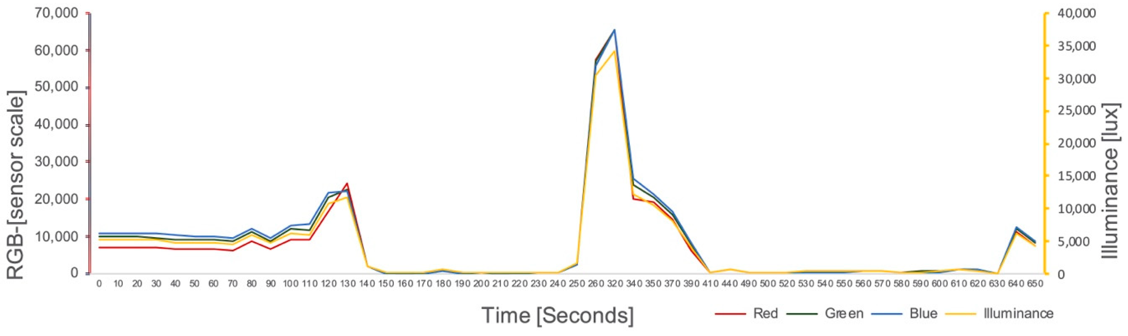
Initially, our study used the above equation in the IDE code for the calculation of radiance from the three primary colors of light. The TCS34725 was used for detection of red, blue, and green bands. Further data included color temperature and illuminance. After overlaying the graphs, it was outlined that the r, g, b readings follow the illuminance pattern (Figure 8). This means the sensor readings and illuminance have a direct relationship.
The RGB sensor readings of 0–65535 were distributed into 16-bit segments for each color. After conversion of the r, g, b scale to 8-bits (0–255), the results were similar to the irradiance reading from illuminance through the estimated value of “0.0079 W/m2 per lux” (Figure 9). The reason for slight differences in peak values is considered to be due to the different techniques used for estimation. Also, the scales are for two different units of solar radiation, i.e., radiance in comparison to irradiance.
The photometric sensors used in the prototype are IR blocking. The related sensors must be added in the prototype for the addition of IR and UV components of the solar spectrum.
4.4. GPS Data
The global positioning system, used for high precision positioning and navigation, has three progression sectors: the satellite constellation (24 satellites orbiting Earth), ground control network (master control station of the satellites), and user equipment (GPS receivers). The GPS receiver simultaneously calculates its two-dimensional position, velocity, and time by the signal evaluation from a minimum of three pseudo-ranges (satellite data), while altitude can be calculated from a fourth pseudo-range. The quality of fix improves with the higher number of pseudo-ranges used for triangulation [29].
The National Marine Electronics Association (NMEA) defines the communication interface between marine electronic equipment as the standard for GPS communications. The prototype’s GPS module also uses the NMEA format as preferred by most computer programs. The communication data includes real-time positional information.
5. Date/Time and Built-In Memory
The GPS module can be used for timekeeping with its built-in RTC. The output from the module remains in coordinated universal time (UTC), and the user can modify the code to convert to local time zone with daylight savings where applicable. As the prototype data logger is already using an RTC, we can keep the GPS date and time reading in UTC to check the time shifts on the data logger.
The GPS module has a microcontroller; therefore, internal data logging can be accomplished by sending a start command using an external microcontroller. The module can then be detached from the external MCU and independently log 16 h of data on its flash memory. This capability of the module can be exploited in future projects.
6. Validation of Environmental Measurements
The prototype measurements are initially cross-checked with the industrial reference devices to ensure the data quality. The main purpose of this step is to identify the errors linked with the current prototype and to eliminate them in the future. This section compares five modules, as shown in Table 2. The reference devices manufactured by Testo, Li-COR, and Radionova are mentioned as “reference” for simplicity in the graphs and explanations.
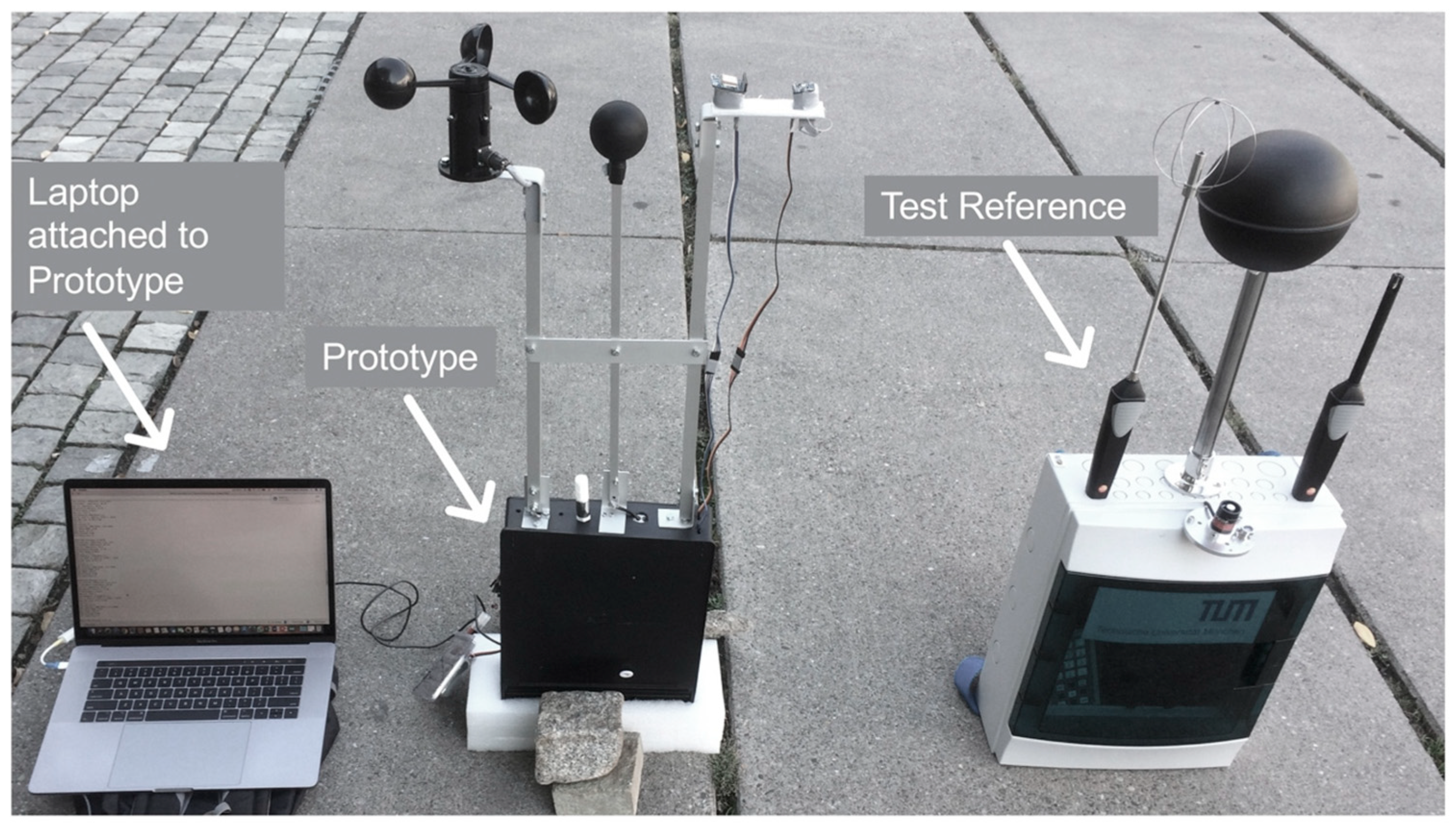
The test was carried out on September 20, 2018, in the courtyard of Technical University of Munich. The devices were fixed to take readings at 4 pm. A computer was connected to the prototype to configure the run-time interims before the test. It was also used to monitor the prototype measurements during the validation. The readings were recorded in ground level and later on the rooftop of the campus. The collection consisted of 97 samples, each taken at 10 s interval. The observers remained approximately 5 m away from the site to minimize the human influence on the data. The setting of the test is shown in Figure 10.
6.1. Globe Temperature
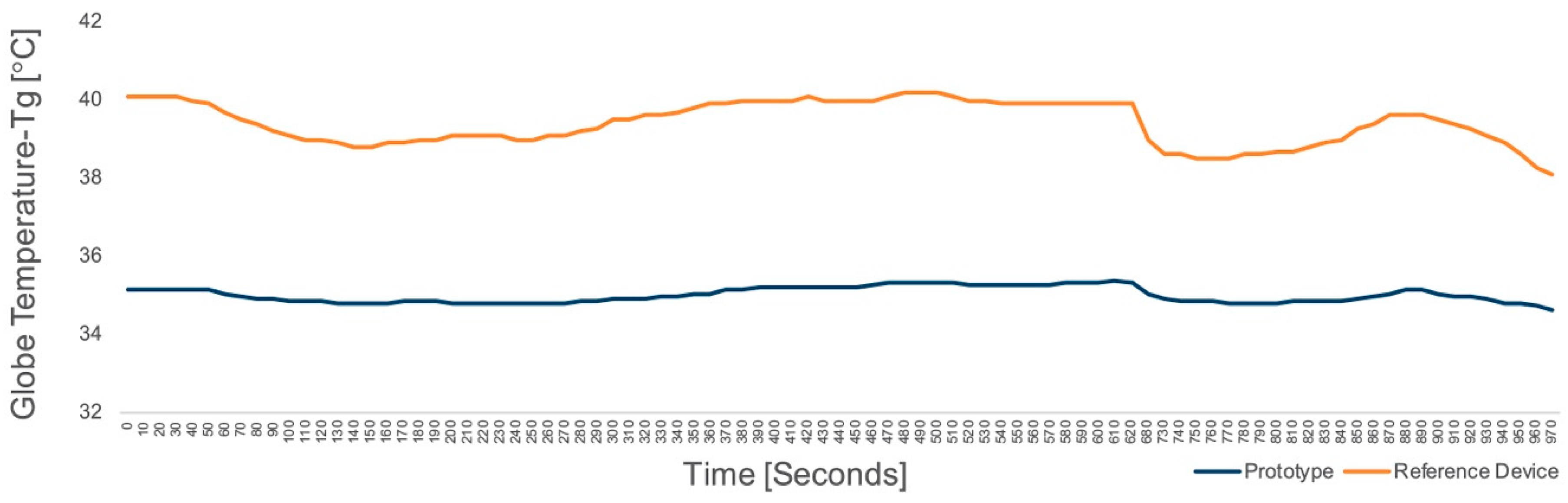
The globe temperature readings from the prototype and reference followed the same patterns. The elevations and depressions of the curves showed similar responses. Nonetheless, the readings from the prototype were lower than that of the reference device. The graph was compared with two vertical legends to focus on the response of each sensor and shift the temperature gap by 4.9 ° (Figure 11). There are numerous reasons for the difference of measurements stated as follows:
- The prototype’s globe temperature sensor has an existing metallic covering, which is further covered by the table tennis ball.
- The prototype and the reference devices were stored in different environments before testing, corresponding to different starting temperatures. This signifies different adoption time to the test environment.
- The sensors have distinctive response time and accuracy.
- The calibration of each sensor is different, which means the prototype’s sensor must be recalibrated according to the test device.
- The material and dimension of each globe are dissimilar. The prototype’s globe is not a conductor (plastic), while the reference sensor is made up of copper and is industrially designed for this purpose.
- The paint on both materials has different ingredients and texture.
The prototype’s paint has not been proposed for heat absorption. Rather, it is a general-purpose paint spray. As the reference sensor has been designed industrially, the properties of the paint must have also been premeditated for optimum resolution.
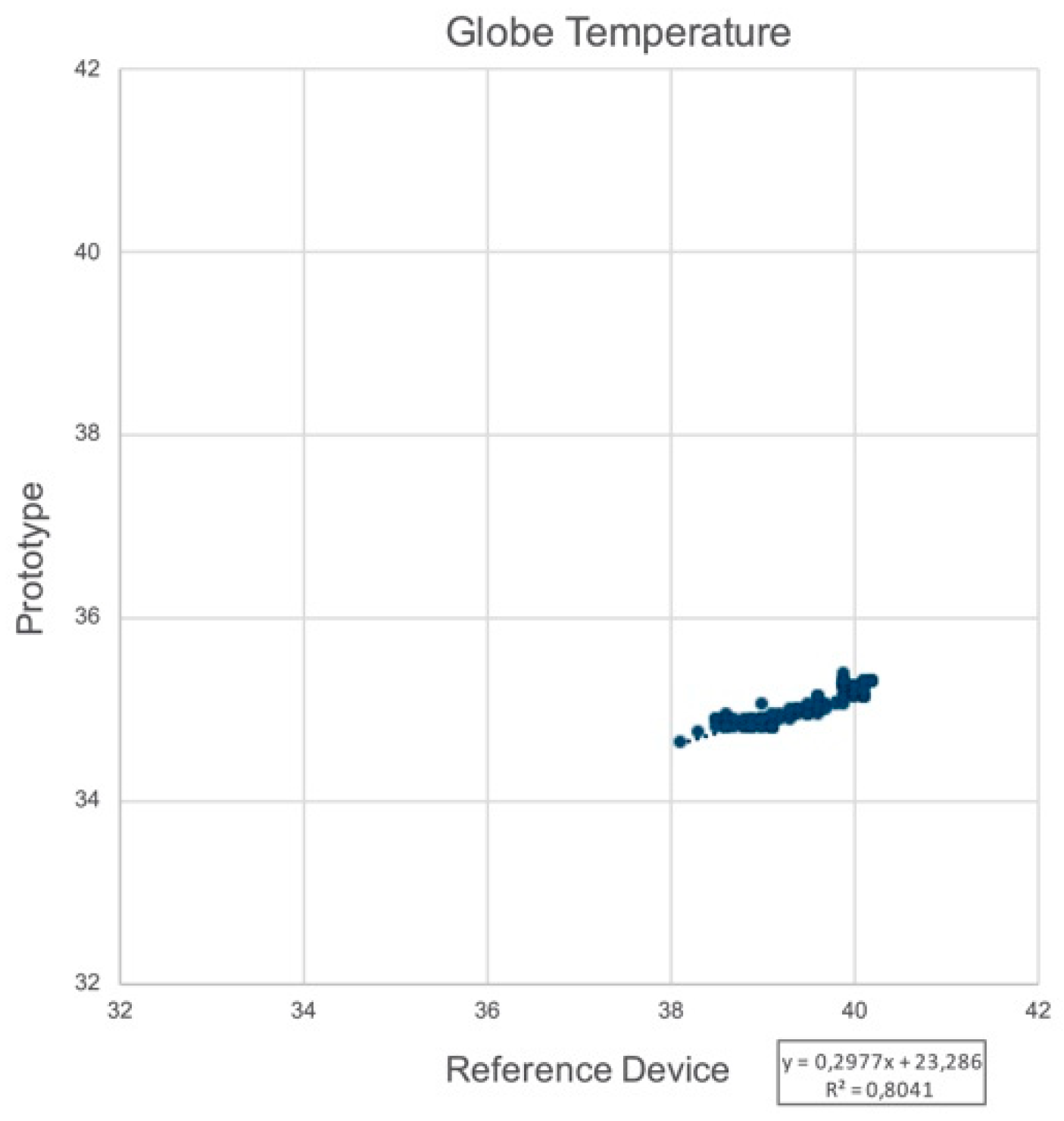
The linear regression trend line for globe temperature of the prototype in context to that of the reference device seems fairly close to 1 (Figure 12).
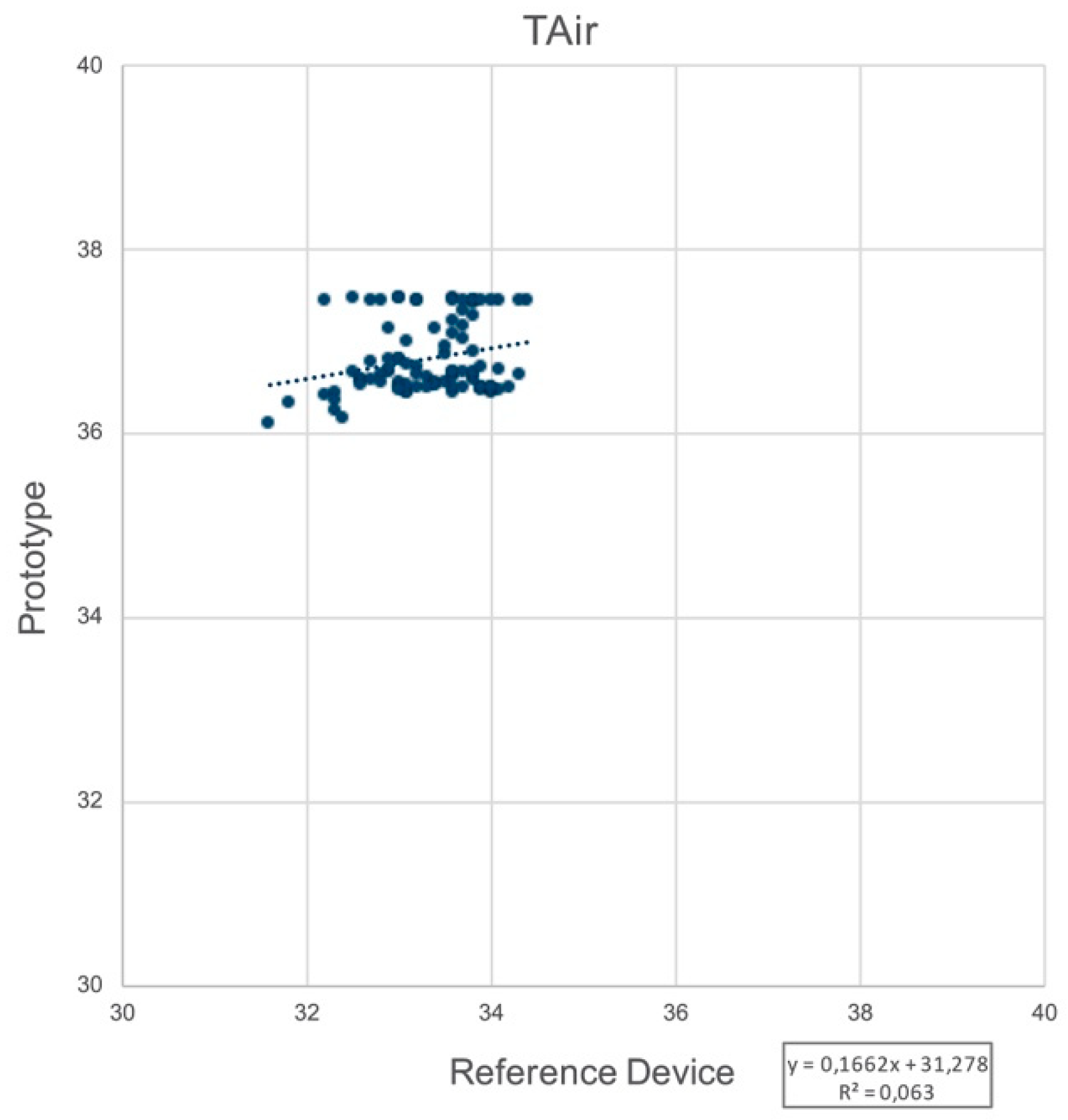
6.2. Air Temperature
The prototype and reference device readings speculate vague similarities, although there are unnecessary temperature fluctuations in the reference device readings (Figure 13). The reasons can be the absence of a protective shield on the reference sensor, resulting in disturbances by the wind. Therefore, the linear regression trend line shows little explanation for air temperature (Figure 14).
The accuracy of the prototype’s air temperature sensor is higher compared to the reference device. Also, the T-air sensors in both devices seem to have different response times. The prototype’s response time depends on the heat conductivity of the sensor substrate between 5 and 30 s. The differences in the comparison due to this dependency were ruled out as the sensor is new and the interval for readings is set to 10 s.
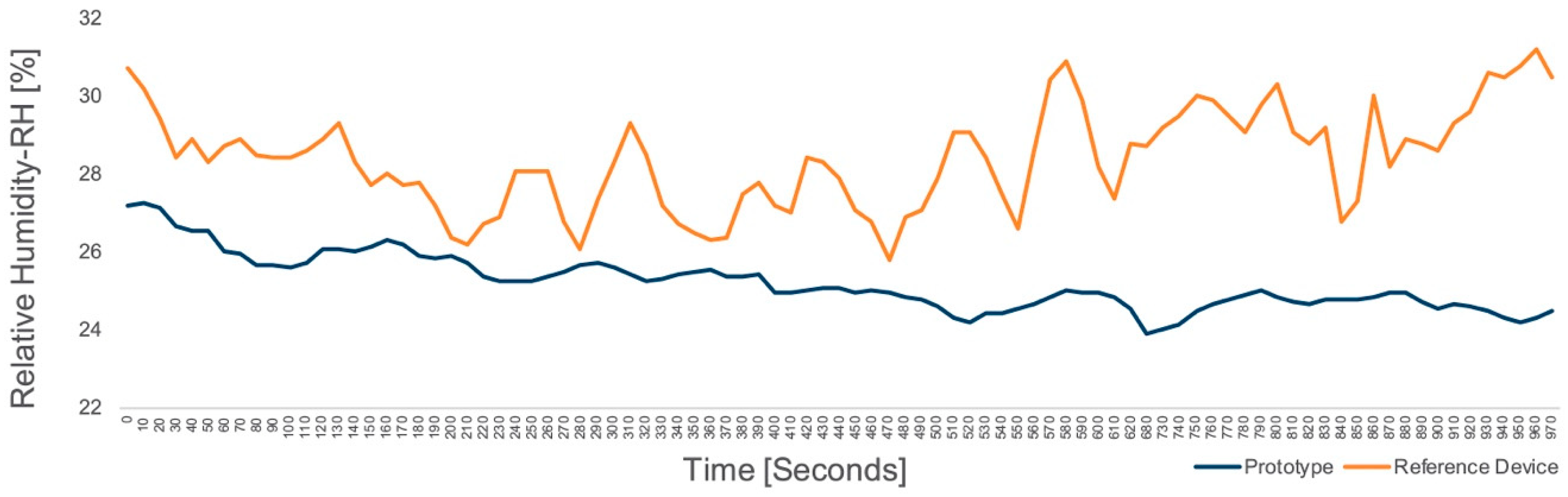
6.3. Relative Humidity
The relative temperature graph of the reference device shows swift changes similar to the air temperature readings in comparison to the prototype. The sensor in the prototype (SHT20) is used for both measurements ( and RH%). Thus, the shield cover is the reason for the gradual changes in the prototype. The marginal gap in the measurement is caused by the difference in the accuracy of both modules (Figure 15). This gap can be concealed by calibration or replacement of the prototype sensor.
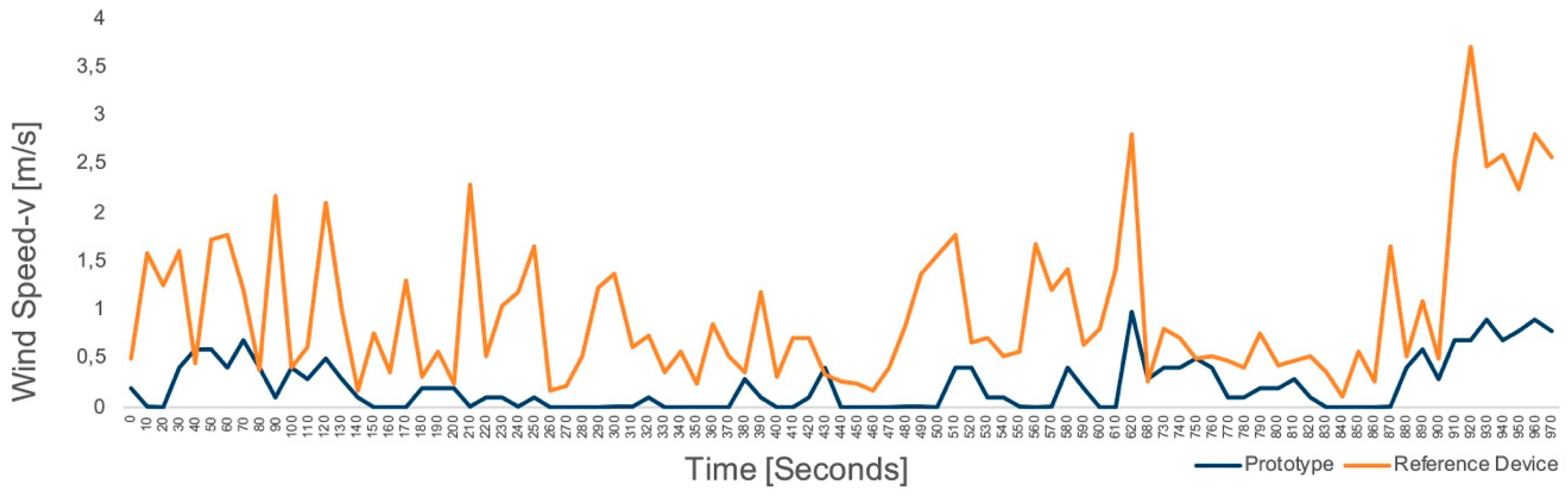
6.4. Wind Speed
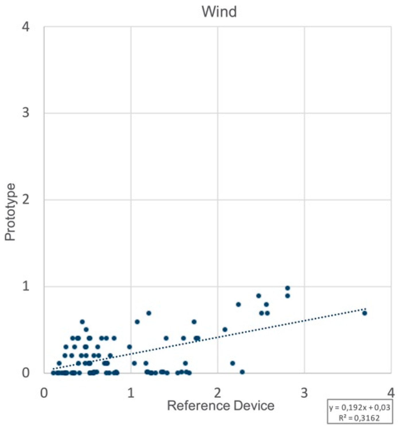
The anemometer of the prototype has a starting speed of 0.4 to 0.8 with a resolution of 0.1 and ±3 system error. On the other hand, the reference airflow probe has an accuracy of ±0.03 . The prototype measurements resemble that of the reference device and follow an almost comparable pattern. However, there is a high difference on the readings scale. The prototype’s interpretations range between 0 and 1.2 , which is relatively lower than the reference device readings (Figure 16). This signifies the need for recalibration of the wind speed to the voltage scale. The linear regression line explains only 31% for wind speed (Figure 17).
There can be a number of factors affecting the differences in both readings, including the vertical distance from the ground and the proximity of the devices from surrounding trees and objects. Therefore, a wind tunnel test could verify the performance of the prototype’s anemometer.
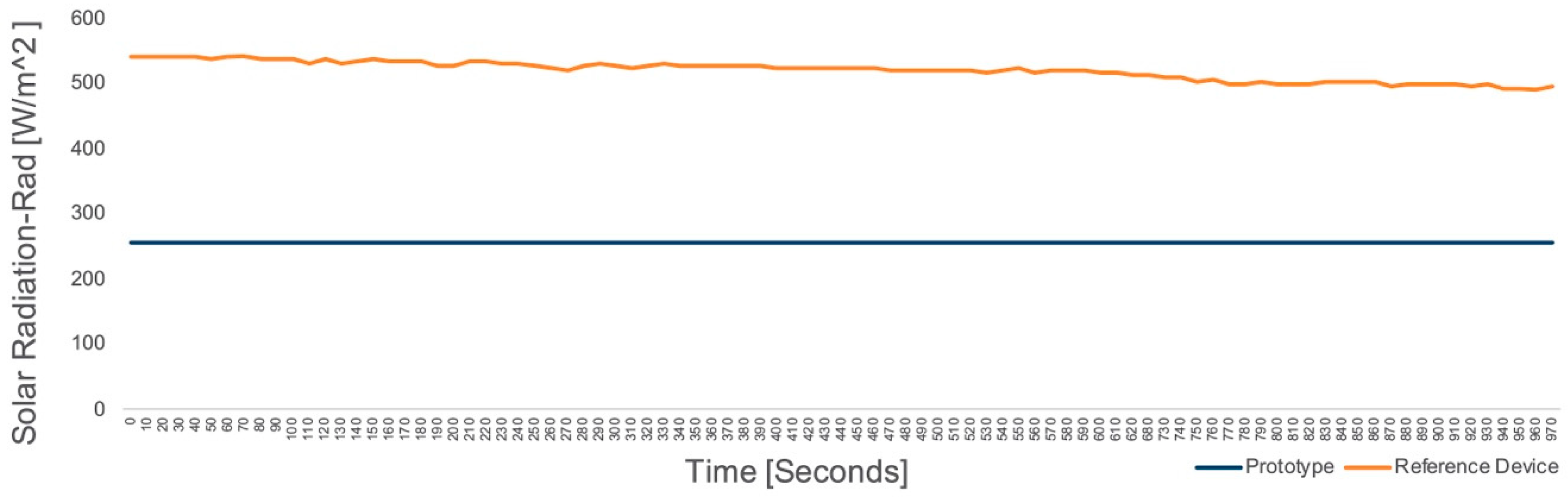
6.5. Solar Radiation
The TCS34725 RGB sensor was chosen for the prototype based on the previously discussed arguments. The main incentive was to reduce the cost as much as possible. However, after comparing the data against the reference sensor, we realized the limitations of this sensor (34,196 lux). Therefore, the capacity of the RGB sensor was deemed insufficient for calculating the solar radiation on a sunny day.
To elaborate, the reference pyranometer recorded between 500 and 560 . On the other hand, the solar radiation readings from the prototype showed a constant 256 values, indicating the maximum limit of the sensor. The result of the test is displayed in Figure 18.
This comparison concludes that our RGB sensor cannot be used in outdoor conditions. However, it can be suitable for calculations under 34,000 lux. The concept could be valid in presence UV and IR sensors provided that the limit of the sensor is beyond 120,000 lux.
6.6. GPS Data
The data acquired from GPS in this test involved location (latitude and longitude), altitude, and the number of satellites detected. The data received from the reference device included horizontal dilution of precision (HDOP), which depicts the error caused by the relative position of GPS satellites. Fundamentally, the dilution of precision (DOP) assures the quality of the signal and minimizes the positional error. In the GPS observation, the widespread satellites mean good DOP and vice versa. DOP values vary from 1 to 20 (1 > DOP > 20). Values below 1 represent ideal precision, and values greater than 20 denote the most inaccurate GPS readings up to 300 m from the actual position. The main causes of these errors are listed as follows:
- Signal refraction by troposphere and ionosphere;
- The multipath effect i.e., deflection of the signal from building and mountains, etc;
- Satellite time and location (ephemeris). Error in synchronization to the satellite’s atomic clock;
- Equivalent to 30 m positional inaccuracies due to selective availability code (nonexistent after May 2000 A.D.).
Nowadays, GPS differential correction and satellite-based augmentation system (SBAS) are used to precisely read GPS signals.
The accuracy of the reference device is rated within 2.5 m, while that of our prototype is rated below 5 m range. The readings from both devices seem fairly precise, but the prototype performed marginally better. The actual performances of both devices have been illustrated in Figure 19 for additional explanation.
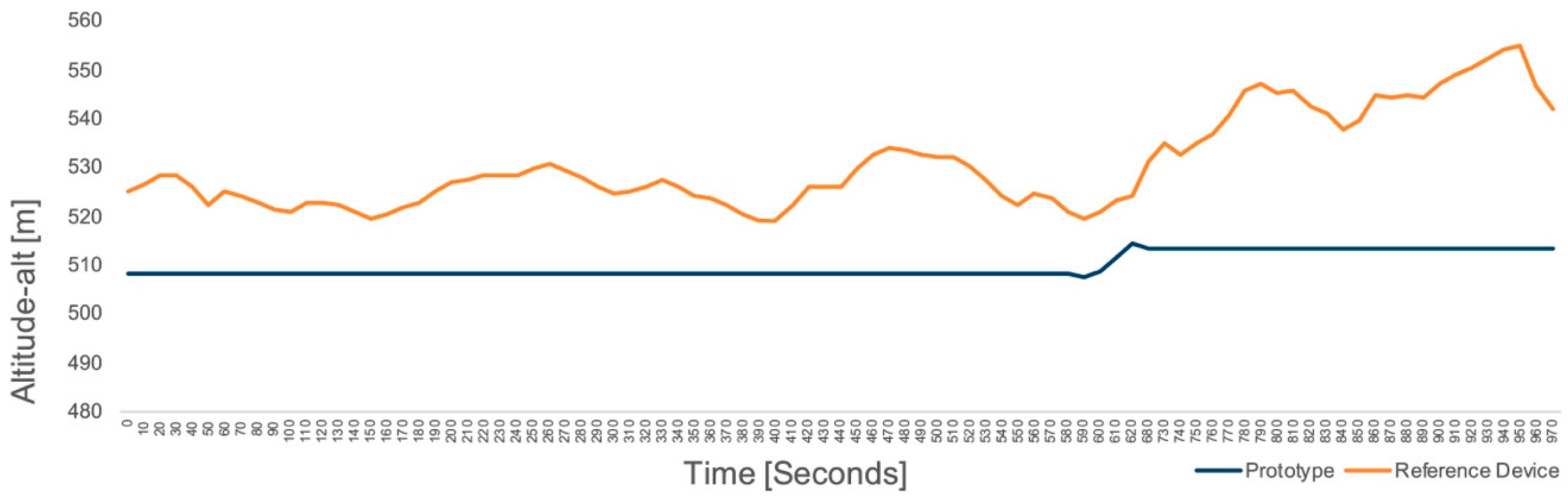
The altitude of the test site on the map is 517 m. The elevation was altered once during the test. The graph from the prototype approves slight inclination from 508.5 to 516.5 m at the third segment of the test. The readings from the reference device appear continuously wavering roughly between 519 to 535 m in the beginning and 530 to 555 m after the level change (Figure 20). Although the change in level shifts was observed by both devices, the readings from the prototype proved to be smoother compared to the reference device.
The number of satellites detected by the prototype remained between 10 and 11 without loss of connection. Both devices had a similar performance for discovering the pseudoranges, whereas the reference device detected the maximum pseudoranges (Figure 21).
It is also necessary to discuss that both of the GPS devices need a certain amount of time to get a signal fix. Fix defines the connection with satellites and the first step for receiving data including 3D location, time, and speed of motion.
6.7. Data Logger
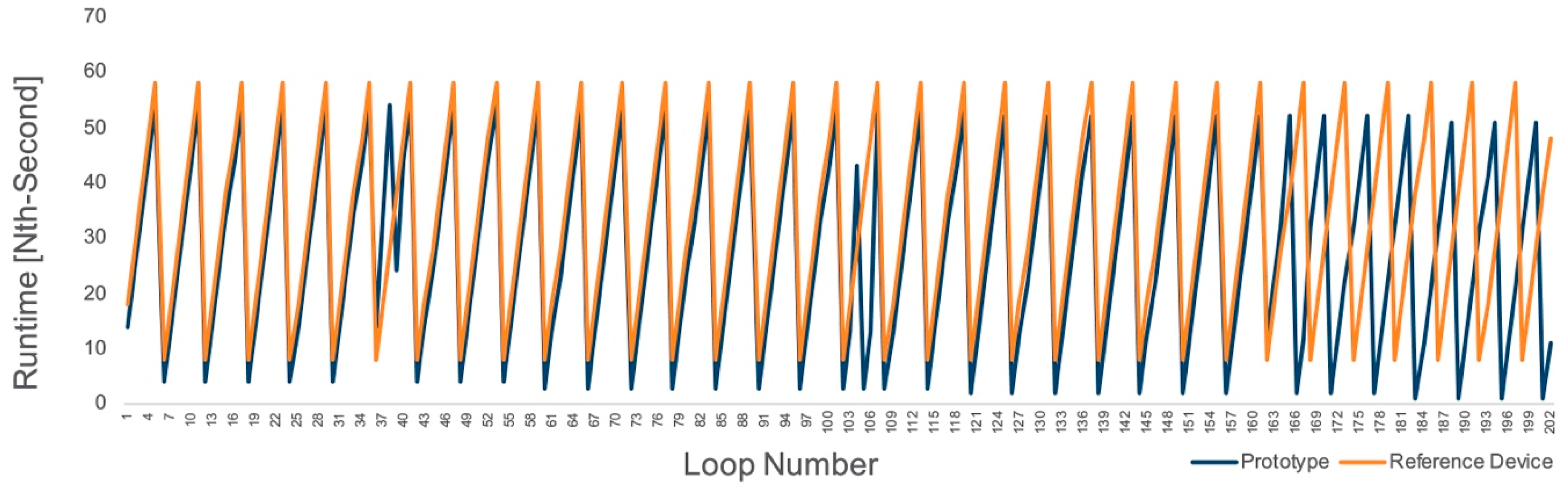
In the early stages of prototyping, short data collection intervals were introduced for testing each sensor. These intervals were programmed using the delay code at the end of the loop segment. As the code became larger, the need for higher intervals was intuited to log all sensor data in one block. The problem with the delay function has been that it pauses the microcontroller’s overall function for the directed span of time, which is not favorable for multitasking projects.
Therefore, the next option was to induce interruptions using a timekeeper function for the thousandth fraction of a second. However, a few microseconds of delay after each loop is still possible due to the following:
- The response time of sensors,
- The time spent on writing the measurements on the serial monitor and the SD card,
- The processing delay, etc.
The prototype readings shifted one second earlier in 37th, 103rd, and 166th loop (Figure 22). This detail remained unnoticed in most cases. It was revealed that even by using “micros ()” function, the prototype intervals logged ahead after a few hundred seconds. For the outdoor comfort analysis, this shift of time may not be a huge concern. The runtime comparison showed much stable data logging with the reference device paralleled to a slightly disturbed pattern (glitch) in the prototype.
7. Mapping of the Georeferenced Data
In this section, the prototype was examined through a climate walk for georeferenced data collection. As the outdoor environments are beyond human control, the tolerance against these conditions is higher compared to indoor scenarios. A suitable approach would be to map indices like the UTCI to account for a wide range of acceptability in thermal comfort.
According to the definition, “UTCI is the air temperature of the reference condition causing the same model response as actual conditions”. The expression includes the meteorological input, the physiological model, and the clothing model to get a dynamic response model. The main factors are air temperature, relative humidity, wind speed, mean radiant temperature, solar irradiance, metabolic rate, and clothing factor. Some supplementary information (i.e., reference to the climate zone, personal background, and physiological data) will enhance the understanding of an individual’s perception of comfort in different environmental situations.
For this assessment, we used the technique from previous research for data plotting on the path. The Grasshopper platform was used for this purpose. The plugins included Ladybug Tools (to calculate the UTCI), @it (to import shapefiles of the buildings and streets, imported from OpenStreetMap and treated with ArcGIS), Lunchbox (to read the files from the data logger), and GHPython (for mathematical calculations and connecting different data types) [30].
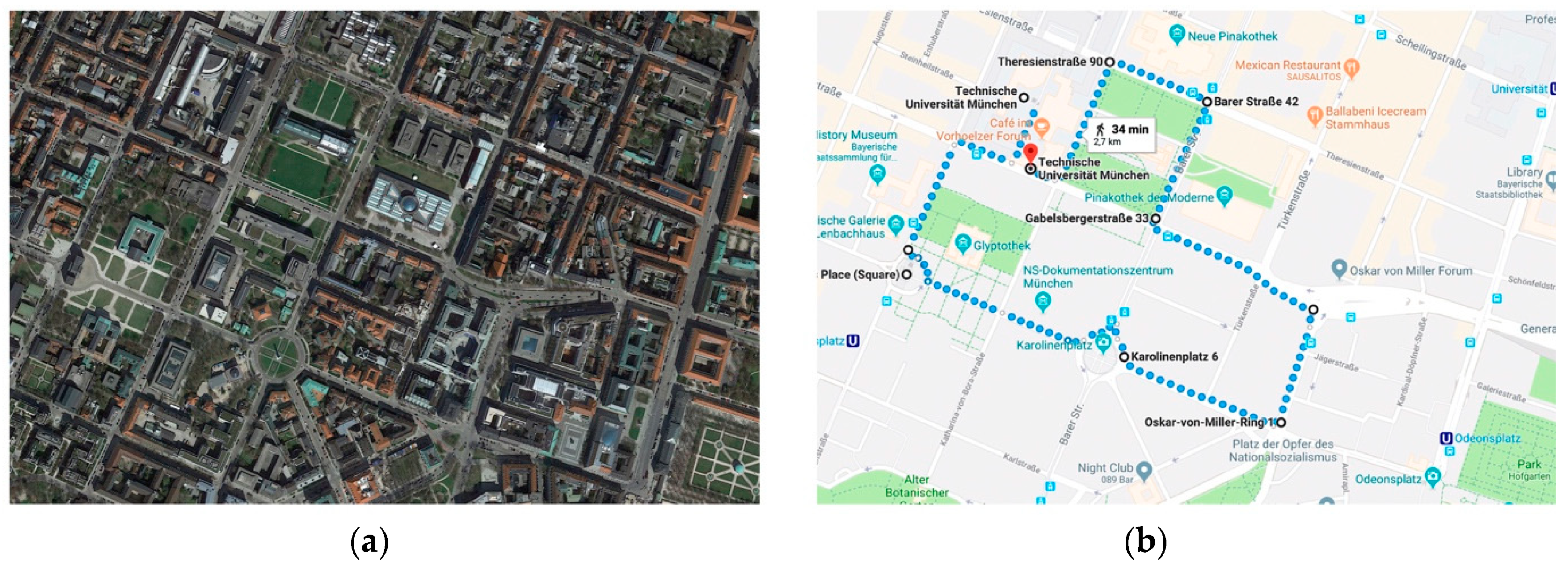
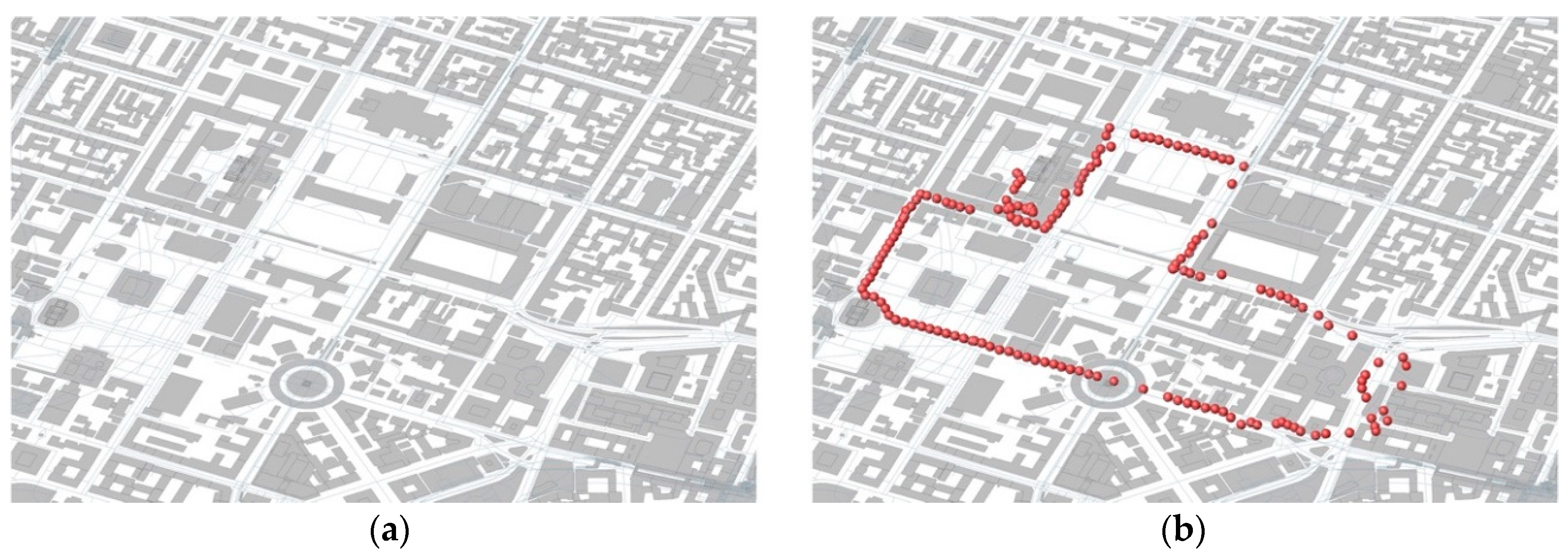
The observation district was Maxvorstadt, Munich. The climate walk route was covered in approximately 35 min. An overview of the selected district is shown in Figure 23. The GPS plot shows precise patterns for geolocation apart from some negligible deviations near the Oscar von Miller Forum. This implies that the GPS readings were accurate enough to ignore the path correction procedures. All the sensor readings were mapped, including the calculations for the MRT and the UTCI (Figure 23, Figure 24, Figure 25, Figure 26, Figure 27, Figure 28, Figure 29, Figure 30 and Figure 31).
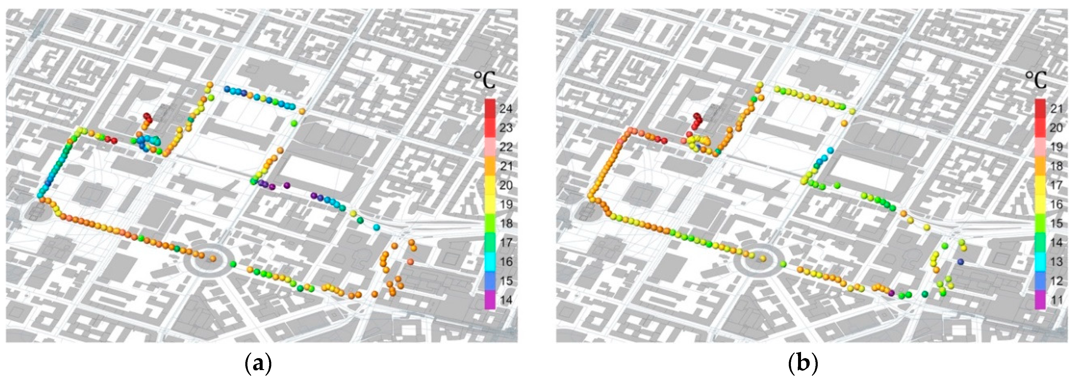
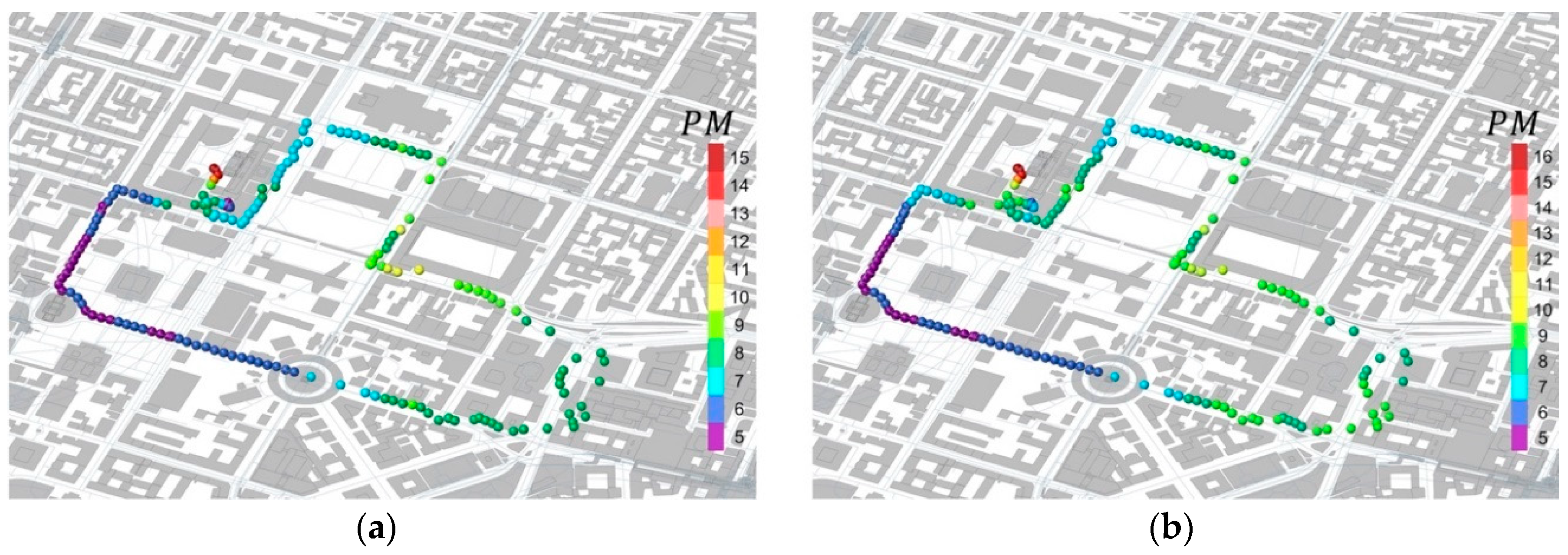
The UTCI map showed a range between 11 and 21 °, indicating no thermal stress. The noise level showed moderation between a few quiet readings of 30 dB to a maximum of 80 dB, while the particulate matter readings for both PM2.5 and PM10 showed a maximum of 16 , which translates to good air quality.
The assessment shows that all the sensors are functional. However, the addition of a pyranometer is necessary to enhance the description of UTCI.
8. Conclusions
This study proposes an Arduino-based toolkit to acquire environmental data with the focus on outdoor comfort assessment techniques. The assembled prototype is a derivative of open-source technologies equipped with the most relevant environmental sensors in terms of cost and performance.
The incentive was to construct a prototype that could be easily deployed in the field. Therefore, four main resolutions were made: the hardware assembly, software programming, data collection, and the application.
Through the prototyping process, we encountered two main limitations for the employed sensors. The first constraint was the range-dependent accuracy of the anemometer, where we found that the module was not reasonably sensitive below 0.8 m/s. This restriction can be reduced by employing a hot wire and thermistor anemometer. The second issue that we came up with was the conversion of photometric values to estimate solar radiation due to the unavailability of low-cost pyranometer. Previous studies have inspired our approach, such as the calculation of solar radiation without a pyranometer. Although the initial idea was to include UV and IR sensors, we found that our target was not achievable under clear-sky conditions with the selected modules due to maximum threshold limitation of the RGB and illuminance sensors. The solution could be to use a silicon pyranometer with a UV sensor. The addition of a pyranometer to the toolkit can provide equitable data to assess transient outdoor conditions.
Further applications of the developed kit can be the accumulation of sky-view factor through GPS readings to understand the effects of urban structures on human comfort and the prediction of microclimatic patterns.
The future use of the developed prototype can be divided into two domains. The first is to assess and map georeferenced transient human comfort to find correlations between the built environment and pedestrian well-being. The second purpose could be the implantation of affordable and fairly accurate environmental sensors in a broader scale in cities to collect, map, and evaluate ambient sensing data.
Author Contributions
The research article is the result of a master thesis of postgraduate course ClimaDesign at Technical University of Munich carried out by Ahmad Saleem Nouman. and supervised by the other authors.
Funding
This work was supported by the German Research Foundation (DFG) and the Technical University of Munich (TUM) in the framework of the Open Access Publishing Program.
Conflicts of Interest
We confirm that the authors faced no conflicts of interest.
References
- Chokhachian, A.; Santucci, D.; Auer, T. A human-centered approach to enhance urban resilience, implications and application to improve outdoor comfort in dense urban spaces. Buildings 2017, 7, 113. [Google Scholar] [CrossRef]
- Kim, Y.-H.; Baik, J.-J. Maximum urban heat island intensity in seoul. J. Appl. Meteorol. 2002, 41, 651–659. [Google Scholar] [CrossRef]
- Kolokotroni, M.; Giridharan, R. Urban heat island intensity in london: An investigation of the impact of physical characteristics on changes in outdoor air temperature during summer. Sol. Energy 2008, 82, 986–998. [Google Scholar] [CrossRef]
- Tumini, I.; Rubio-Bellido, C. Measuring climate change impact on urban microclimate: A case study of concepción. Procedia Eng. 2016, 161, 2290–2296. [Google Scholar] [CrossRef]
- Ebrahimabadi, S. Outdoor Comfort in Cold Climates: Integrating Microclimate Factors in Urban Design. Ph.D. Thesis, Comprehensive Summary, Luleå Tekniska Universitet, Luleå, Sweden, 2015. [Google Scholar]
- Yang, B.; Olofsson, T.; Nair, G.; Kabanshi, A. Outdoor thermal comfort under subarctic climate of north sweden—A pilot study in umeå. Sustain. Cities Soc. 2017, 28, 387–397. [Google Scholar] [CrossRef]
- Chokhachian, A.; Santucci, D.; Vohlidka, P.; Auer, T. Framework for defining a transient outdoor comfort model in dense urban spaces, processes & findings. In 7th International Doctoral Conference, Architecture and Urbanism: Contemporary Research; Faculty of Architecture CTU: Prague, Czech Republic, 2017; pp. 51–54. [Google Scholar]
- Masson, V.; Marchadier, C.; Adolphe, L.; Aguejdad, R.; Avner, P.; Bonhomme, M.; Bretagne, G.; Briottet, X.; Bueno, B.; de Munck, C.; et al. Adapting cities to climate change: A systemic modelling approach. Urban Clim. 2014, 10, 407–429. [Google Scholar] [CrossRef]
- Corburn, J. Reconnecting with our roots: American urban planning and public health in the twenty-first century. Urban Aff. Rev. 2007, 42, 688–713. [Google Scholar] [CrossRef]
- Fanger, P.O. Thermal Comfort. Analysis and Applications in Environmental Engineering; Danish Technical Press: Copenhagen, Denmark, 1970; 244p. [Google Scholar]
- Mazhar, N.; Brown, R.D.; Kenny, N.; Lenzholzer, S. Thermal comfort of outdoor spaces in lahore, pakistan: Lessons for bioclimatic urban design in the context of global climate change. Landsc. Urban Plan. 2015, 138, 110–117. [Google Scholar] [CrossRef]
- Cheshire, W.P. Thermoregulatory disorders and illness related to heat and cold stress. Auton. Neurosci. 2016, 196, 91–104. [Google Scholar] [CrossRef]
- Nunez, M.; Oke, T.R. The energy balance of an urban canyon. J. Appl. Meteorol. 1977, 16, 11–19. [Google Scholar] [CrossRef]
- Mauree, D.; Blond, N.; Clappier, A. Multi-scale modeling of the urban meteorology: Integration of a new canopy model in the wrf model. Urban Clim. 2018, 26, 60–75. [Google Scholar] [CrossRef]
- Salamanca, F.; Martilli, A.; Tewari, M.; Chen, F. A study of the urban boundary layer using different urban parameterizations and high-resolution urban canopy parameters with WRF. J. Appl. Meteorol. Climatol. 2011, 50, 1107–1128. [Google Scholar] [CrossRef]
- Fuentes, M.; Vivar, M.; Burgos, J.M.; Aguilera, J.; Vacas, J.A. Design of an accurate, low-cost autonomous data logger for pv system monitoring using Arduino™ that complies with IEC standards. Sol. Energy Mater. Sol. Cells 2014, 130, 529–543. [Google Scholar] [CrossRef]
- Ali, A.S.; Zanzinger, Z.; Debose, D.; Stephens, B. Open source building science sensors (OSBSS): A low-cost Arduino-based platform for long-term indoor environmental data collection. Build. Environ. 2016, 100, 114–126. [Google Scholar] [CrossRef]
- Baker, E. Open source data logger for low-cost environmental monitoring. Biodivers. Data J. 2014, 2, e1059. [Google Scholar] [CrossRef]
- Badamasi, Y.A. The Working Principle of an Arduino. In Proceedings of the 2014 11th International Conference on Electronics, Computer and Computation (ICECCO), Abuja, Nigeria, 29 September–1 October 2014; pp. 1–4. [Google Scholar]
- Błażejczyk, K.; Broede, P.; Fiala, D.; Havenith, G.; Holmér, I.; Jendritzky, G.; Kampmann, B.; Kunert, A. An introduction to the universal thermal climate index (UTCI). Geog. Pol. 2013, 86, 5–10. [Google Scholar] [CrossRef]
- Jendritzky, G.; de Dear, R.; Havenith, G. Utci—Why another thermal index? Int. J. Biometeorol. 2012, 56, 421–428. [Google Scholar] [CrossRef]
- Jendritzky, G.; Havenith, G.; Weihs, P.; Batchvarova, E. Towards a Universal Thermal Climate Index UTCI for Assessing the Thermal Environment of the Human Being; Final Report COST Action; COST (European Cooperation in Science and Technology): Brussels, Belgium, 2009; pp. 1–26. [Google Scholar]
- Herrmann, J.; Matzarakis, A. Mean radiant temperature in idealised urban canyons—Examples from freiburg, germany. Int. J. Biometeorol. 2012, 56, 199–203. [Google Scholar] [CrossRef]
- Thorsson, S.; Lindberg, F.; Eliasson, I.; Holmer, B. Different methods for estimating the mean radiant temperature in an outdoor urban setting. Int. J. Climatol. 2007, 27, 1983–1993. [Google Scholar] [CrossRef]
- Gueymard, C. A two-band model for the calculation of clear sky solar irradiance, illuminance, and photosynthetically active radiation at the earth’s surface. Sol. Energy 1989, 43, 253–265. [Google Scholar] [CrossRef]
- Iqbal, M. Chapter 10—Configuration factors. In An Introduction to Solar Radiation; Iqbal, M., Ed.; Academic Press: Cambridge, MA, USA, 1983; pp. 295–301. [Google Scholar]
- Bass, M.; Stryland, E.W.V.; Williams, D.R. Handbook of Optics; McGraw-Hill: New York, NY, USA, 1995; Volume 2. [Google Scholar]
- Compagnon, R. Radiance: A Simulation Tool for Daylighting Systems; The Martin Centre for Architectural and Urban Studies, University of Cambridge Department of Architecture: Cambridge, UK, 1997. [Google Scholar]
- Chapman, L.; Thornes, J.E.; Bradley, A.V. Sky-view factor approximation using GPS receivers. Int. J. Climatol. 2002, 22, 615–621. [Google Scholar] [CrossRef]
- Chokhachian, A.; Ka-Lun Lau, K.; Perini, K.; Auer, T. Sensing transient outdoor comfort: A georeferenced method to monitor and map microclimate. J. Build. Eng. 2018, 20, 94–104. [Google Scholar] [CrossRef]
Figure 1.
The schematic hardware connection of the model.

Figure 2.
The process of testing environmental sensors.

Figure 3.
Wiring and schematic diagram of the conclusive model (Fritzing).

Figure 4.
The model’s exterior frame and setting of the components.

Figure 5.
An outline of data acquisition system.

Figure 6.
Globe temperature, air temperature, and relative humidity curves.

Figure 7.
Globe temperature, wind speed, and mean radiant temperature curves.

Figure 8.
Comparison of red, green, blue (RGB) colors and illuminance.

Figure 9.
Approximation of solar radiation with RGB and lux sensor.

Figure 10.
Validation setup with prototype and the test reference.

Figure 11.
Validation graph for globe temperature.

Figure 12.
The linear regression graph for globe temperature.

Figure 13.
Validation graph for air temperature.

Figure 14.
The linear regression graph for air temperature.

Figure 15.
Validation graph for relative humidity.

Figure 16.
Validation graph for wind speed.

Figure 17.
The linear regression graph for wind speed.

Figure 18.
Validation graph for solar radiation.

Figure 19.
Georeferencing accuracy visualized over campus map; GPS location mapped with Grasshopper3D.
Figure 19.
Georeferencing accuracy visualized over campus map; GPS location mapped with Grasshopper3D.

Figure 20.
Validation graph altitude.

Figure 21.
Validation graph for number of pseudoranges.

Figure 22.
Validation graph for data logger.

Figure 23.
(a) Region of assessment in city of Munich; (b) the route.

Figure 24.
(a) Figure ground map; (b) GPS signals over the path.

Figure 25.
(a) Elevation of the path (m); (b) walking ground speed (km/h).

Figure 26.
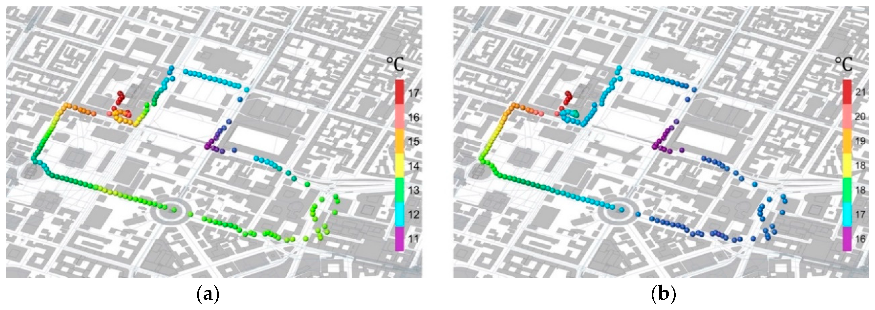
Transient temperature maps: (a) globe temperature (°C); (b) air temperature (°C).

Figure 27.
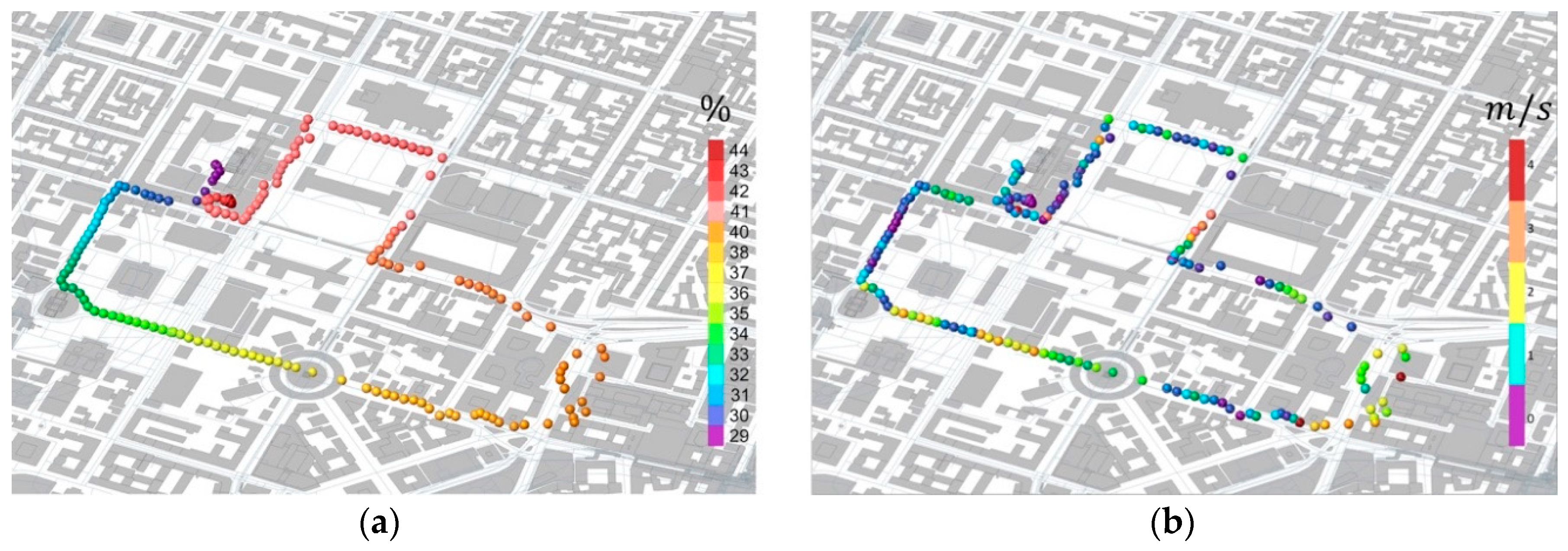
(a) Relative humidity (%); (b) wind speed (m/s).

Figure 28.
(a) Solar radiation (w/m2); (b) noise level maps (dB).

Figure 29.
(a) Mean radiant temperature (°C); (b) universal thermal climate index maps (°C).

Figure 30.
Particulate matter maps: (a) PM 2.5; (b) PM 10.

Figure 31.
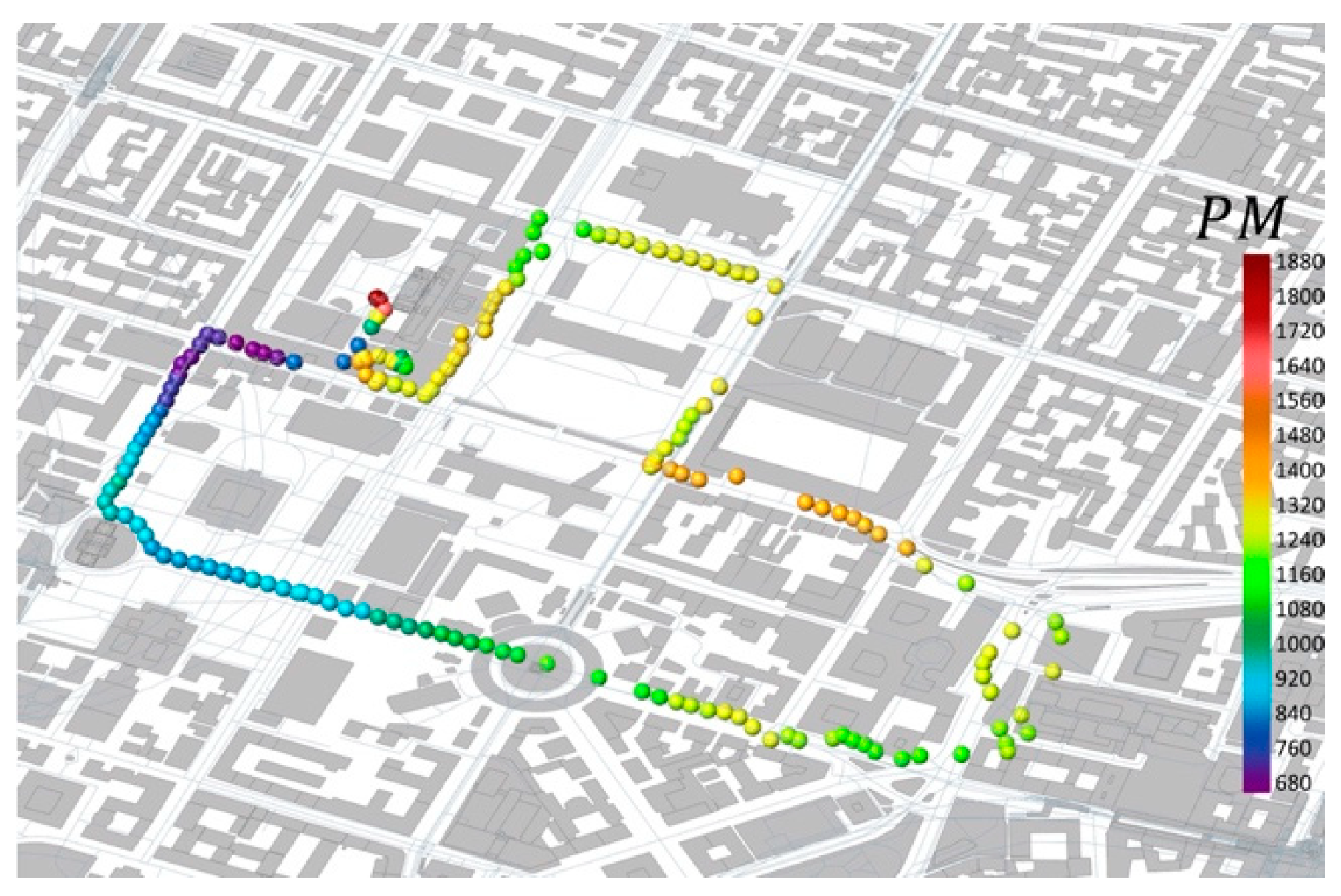
Map for detected particles >0.3 micrometer/0.1 L.


Table 1.
List of components for the Weather-Gear prototype.
| Component | Representation | Description | Range | Accuracy |
|---|---|---|---|---|
| Arduino Mega 2560 |  | Microcontroller unit | − | − |
| Data logger |  | Arduino shield | − | − |
| DS18B20 |  | Temperature () | −55 to +125 ° | ±0.5 ° |
| SHT20 |  | Temperature Humidity | −40 to +125 ° 0–100 | ± 0.3 ° ± 3 |
| TSL2561 |  | Luminosity | 0.1−40,000 lux | − |
| TCS34725 |  | RGB | − | − |
| SEN0170 |  | Wind ( | 0− | ±3% |
| Adafruit Ultimate |  | GPS breakout | 22 satellites | >3 |
| SEN-14262 |  | Sound detector | − | − |
| PMS5003 |  | Particulate matter | 0.3 −10 | 98 (at 0.5 ) |
| ESP-01 |  | Wi-Fi module | ||
| Feather Huzzah |  | Microcontroller unit with built-in Wi-Fi | − | − |
| DHT11 |  | Temperature Humidity () | 0−50 ° 20–80 | ±2.0 ° ±5 |
| Liquid crystal display (LCD) 1602 |  | 16×02 Alphanumerical display | − | − |
Table 2.
Accuracy of components (prototype and reference sensors).
| Parameters | Prototype | Accuracy | Reference Sensors | Accuracy |
|---|---|---|---|---|
| Temperature () | DS18B20 | ±0.5 ° | TESTO 06020743 | ±1.0 ° |
| Temperature | SHT20 | ±0.3 ° | TESTO Probe 06280143 | ±0.5 ° |
| Humidity | SHT20 | ±3 | TESTO Humidity Probe 06369743 | ±1.0 |
| Radiation | TCS34725 | − | LI-COR LI-200R | 0.183 |
| Wind () | SEN0170 | ±3% | TESTO Air Flow Probe 06280143 | ±0.03 |
| GPS | Adafruit Ultimate | >3 | RADIONOVA (RF) Antenna | − |
© 2019 by the authors. Licensee MDPI, Basel, Switzerland. This article is an open access article distributed under the terms and conditions of the Creative Commons Attribution (CC BY) license (http://creativecommons.org/licenses/by/4.0/).
Share and Cite
MDPI and ACS Style
Nouman, A.S.; Chokhachian, A.; Santucci, D.; Auer, T. Prototyping of Environmental Kit for Georeferenced Transient Outdoor Comfort Assessment. ISPRS Int. J. Geo-Inf. 2019, 8, 76. https://doi.org/10.3390/ijgi8020076
AMA Style
Nouman AS, Chokhachian A, Santucci D, Auer T. Prototyping of Environmental Kit for Georeferenced Transient Outdoor Comfort Assessment. ISPRS International Journal of Geo-Information. 2019; 8(2):76. https://doi.org/10.3390/ijgi8020076
Chicago/Turabian StyleNouman, Ahmad Saleem, Ata Chokhachian, Daniele Santucci, and Thomas Auer. 2019. "Prototyping of Environmental Kit for Georeferenced Transient Outdoor Comfort Assessment" ISPRS International Journal of Geo-Information 8, no. 2: 76. https://doi.org/10.3390/ijgi8020076
Note that from the first issue of 2016, this journal uses article numbers instead of page numbers. See further details here.