Deriving Animal Movement Behaviors Using Movement Parameters Extracted from Location Data


1
Faculty of Science and Technology, Norwegian University of Life Sciences, Drøbakveien 31, NO-1433 Ås, Norway
2
Norwegian Institute of Bioeconomy Research, Postboks 115, NO-1431 Ås, Norway
*
Author to whom correspondence should be addressed.
ISPRS Int. J. Geo-Inf. 2018, 7(2), 78; https://doi.org/10.3390/ijgi7020078
Submission received: 14 December 2017
/
Revised: 9 February 2018
/
Accepted: 18 February 2018
/
Published: 24 February 2018
(This article belongs to the Special Issue Discovery and Prediction of Moving Objects in Databases using GIS-based Tools)
Abstract
:We present a methodology for distinguishing between three types of animal movement behavior (foraging, resting, and walking) based on high-frequency tracking data. For each animal we quantify an individual movement path. A movement path is a temporal sequence consisting of the steps through space taken by an animal. By selecting a set of appropriate movement parameters, we develop a method to assess movement behavioral states, reflected by changes in the movement parameters. The two fundamental tasks of our study are segmentation and clustering. By segmentation, we mean the partitioning of the trajectory into segments, which are homogeneous in terms of their movement parameters. By clustering, we mean grouping similar segments together according to their estimated movement parameters. The proposed method is evaluated using field observations (done by humans) of movement behavior. We found that on average, our method agreed with the observational data (ground truth) at a level of 80.75% ± 5.9% (SE).
1. Introduction
Animal movement analysis is being revolutionized by the increasing positional accuracy and temporal frequency of tracking devices, such as ARGOS tags, RFID (Radio Frequency IDentification) tags, Geotags, and GNSS (Global Navigation Satellite System) tags [1]. Inexpensive and ubiquitous positioning technologies and the development of methods to characterize and classify movement behavioral states from captured location data have received considerable attention in movement ecology.
Given an animal movement path [2,3,4], as a sequence of time-stamped locations, we focus on how to make inferences about animal movement behavior. Where and when does the animal engage in a specific movement behavior, and how does the movement behavior change over time?
Quantities like speed, step length (straight-line distance between successive locations), direction, and turning angle (change of direction between successive steps) that can be calculated from the raw location data are called movement parameters [5,6]. The movement parameters can be good proxies for movement behavioral states along an animal movement path [4].
The main research goal is this: Given sampled locations of an animal movement path, we aim at partitioning the movement path according to changes in movement behavior. Movement behavior is defined based on various combinations of the movement parameters, including turning angle and speed. According to [7], movement behaviors can be (i) resting (low mean turning angle and low mean speed), (ii) walking (low mean turning angle and high mean speed), (iii) foraging (high mean turning angle and low mean speed), and possibly (iv) undefined movement behavior (high mean turning angle and high mean speed). The movement behavior of high turning angle and high speed is unlikely, as demonstrated by the Classification and Regression Tree method proposed in [8].
The proposed framework for detecting movement behavioral states according to changes in the movement parameters consists of two parts: (i) Using a slightly modified version of the recently developed behavioral change point analysis (BCPA) method [5,9], we partition an individual trajectory into segments of homogeneous movement parameters. (ii) Using the Kolmogorov–Smirnov distance metric, we compute a distance matrix for all pairs of segments, in order to generate an agglomerative hierarchical clustering model of the segments [10].
The remaining parts of the paper are structured as follows. We start by reviewing some relevant animal movement behavioral studies, which attempt to distinguish between different movement behavioral states based on location data. Then we describe our dataset and the field observations. Finally, we describe our methodological approach, including the modified version of BCPA and the proposed hierarchical clustering method, and validate the resulting model, using the field observations as ground truth.
2. Background
Recent developments in tracking devices and the increasing availability of movement data provide new opportunities for the inference of movement behavior from animal movement paths [4,11,12,13]. There are different approaches for distinguishing movement behaviors from animal movement paths, including statistical modelling, data mining techniques, mixtures of random walk models, and movement-derived parameters [3,4,5,9,14,15,16].
Gurarie et al. [12] group behavioral movement analysis methods into four categories: (1) metric-based, (2) classification and segmentation, (3) phenomenological time series analysis and (4) mechanistic movement modelling. They compare the categories in terms of complexity of the results and the intrinsic differences in the output, using one method from each category.
Edelhoff et al. [4] outline three broad types of research questions that are commonly addressed using path segmentation methods: (1) the quantitative description of movement patterns, (2) the detection of significant change points, and (3) the identification of underlying processes or hidden states.
The first type is based on geometric analysis of movement parameters. The movement paths are split into segments that are assumed to reflect different underlying movement behavior. Movement parameters include mean squared displacement [17], first passage time [18], (multi-scale) straightness index [14] and fractal dimension [19].
State–space modeling is closely related to the latter type, and seems promising. State–space models [16] are models that allow unobservable, true states to be inferred from observed data, by accounting for errors arising from imprecise observations and from stochasticity in the process being studied [20]. Specifying appropriate prior distributions and underlying model parameters for state–space models can be a challenging task for non-experts.
The second, and most interesting type for our framework, assesses movement parameters along the time axis, and identifies the structure or correlation of movement data using time series analysis. Relying on significant change points along the animal movement path, we selected the BCPA method [4,9] to segment the path, taking the temporal autocorrelation of the movement data into account. BCPA is acknowledged in the literature as a good method for segmenting movement paths efficiently, and it is relatively straightforward to implement. The method developed by Zhang et al. [21] is directly comparable to our method, since it also applies BCPA. Zhang et al. [21] used a three-step framework, including BCPA, hierarchical multivariate cluster analysis, and k-means clustering. Hierarchical multivariate cluster analysis is required to determine the number of clusters (k) before doing k-mean clustering. We wanted to consider the overall distribution of the movement parameter values in the clustering process, rather than a specific statistic like central tendency or median as used in [21]. With our approach, we also do not have to worry about seed selection, which k-means is sensitive to.
BCPA, like many segmentation methods (e.g., [22]), only provides information on significant change points along the movement path, without any further ecological context. That is why subsequent analysis (see Section 3.2 below) is required to gain particular insight into the movement behavioral states.
Having found the significant change points along the movement path, the main challenge is to cluster the segments, in order to identify different types of movement behavior. The clustering task includes two important steps: first, an appropriate similarity measure must be chosen, and second, an appropriate algorithm for grouping the observations based on the chosen similarity measure is required.
Several of the proposed trajectory clustering approaches [23,24,25] rely on the similarity of geometric shape, ignoring the temporal dimension. Recent works have developed spatiotemporal similarity measures for trajectory data, considering both the spatial and temporal dimensions [26,27]. As stated in [28], related work on similarity measures for trajectories include time series similarity measures, such as a variation of Minkowski distance (Lp-Norm family) [29], dynamic time warping (DTW) [30], edit distance [31], longest common subsequence (LCSS) [32], geometric shape matching techniques (such as Hausdorff distance) [33], and Fréchet distance [34]. It is worth noting that trajectories may be considered as similar in different respects—they may fully or partly coincide in space, have similar shapes, be fully or partly synchronous, or they may be disjointed in time but with similar movement behavior (speed, acceleration, etc.) [35,36].
We will assume that some unknown probability distribution functions of movement parameters can be used to characterize animal movement behavioral states [3]. The corresponding research goal is therefore to establish the concept of similarity between different animal movement behaviors, based on probability distribution functions estimated from the movement parameters.
3. Methodology
Classifying a heterogeneous trajectory according to movement behavior starts with a segmentation of the trajectory into reasonably homogenous parts, using relevant movement parameters. Then, these segments are grouped according to similarities in movement behavior. In this context, segmentation means the partitioning of a trajectory, T, into an unknown number (l) of sub-trajectories (T1, T2, …, Tl) referred to as segments [4].
In Section 3.1, we demonstrate how to apply the BCPA for trajectory segmentation. In Section 3.2, we explain how hierarchical clustering can be applied to obtain a grouping of the data, yielding satisfactory results for real-world, auto-correlated, high temporal frequency data (see Section 4).
3.1. Behavioral Change Point Analysis (BCPA)
Spatio-temporal autocorrelation is an intrinsic property of animal movement data that separates it from a random set of location data [37]. As the time interval between location observations decreases, the dependency between successive observations increases. In other words, the higher the temporal frequency of position sampling, the stronger the spatio-temporal autocorrelation (function of temporal and spatial distance between observations) [38]. Autocorrelation means that values from observations taken close to each other tend to be either more similar (positive autocorrelation) or less similar (negative autocorrelation) than would be expected from a random arrangement [2]. Nearness can be defined in space (spatial autocorrelation), or in time (temporal autocorrelation), or in both space and time (spatio-temporal autocorrelation).
Our first main goal is to identify points on the animal movement path where significant changes occur in movement behavior. We do not have any a priori assumptions about the number of change points. The temporal correlation (autocorrelation) of the movement parameters has to be considered to avoid spurious change points [12]. According to the guidelines for method selection in [4], “time-series based analysis” is the most appropriate segmentation method for our specific research goal and data. Recently, Gurarie et al. [9] introduced BCPA to statistically determine changes in movement behavioral states along an animal’s movement path. In BCPA, the autocorrelation is modelled explicitly as part of the likelihood function. Changes in the movement behavioral state are identified based on pronounced changes in the movement parameters (in our case, “persistence velocity” and “turning velocity”, see Section 3.1.2 below).
The BCPA identifies changes in movement parameter values across a dataset, by using likelihood comparisons in a moving window over the time series. Within the window, the most likely change point is located according to the Bayesian Information Criterion (BIC) [12], which is a criterion for model selection among a finite set of models [39]. For the mathematical details of BCPA, readers are referred to [9]. For the present analysis, only the principles (without technical details) are required.
3.1.1. Moving Window Size
Choosing the moving window size is an important part of the data analysis, as it drives the resulting segmentation. Exploring the results obtained by using different window sizes is therefore an essential aspect in adapting the methodology for different studies.
The most important statistical assumptions in the modeling of BCPA are the Gaussian error structure and the exponential decay in the autocorrelation. To assess the assumptions of the BCPA, a diagnostic plot should be used both for comparing the residuals to a standard normal distribution and inspecting the autocorrelation function of the residuals [12,40]. Determining the moving window size is a challenge in BCPA. Based on the diagnostic plot of the residuals, BCPA is run with increasing window sizes (including at least 20 samples [9]), in a trial and error fashion, to identify a good value for the size of the moving window (see Section 5, results).
3.1.2. Movement Parameters and Movement Behavior
Movement parameters can be calculated based on either consecutive positions (stepwise) or multiple steps [4]. Most movement parameters are stepwise, including speed, step length, turning angle [41], persistence/turning velocity [9], net/mean squared displacement [17] and first passage time [18]. Sinuosity/tortuosity [42], fractal dimension [19] and multi-scale straightness index [14] are examples of movement parameters that are calculated over multiple steps.
Speed and turning angle are basic movement parameters that can be used to describe and analyze movement paths [6,41]. Laube and Purves [43] investigated how the temporal scale of locational data affects the calculation of movement parameters, such as the speed and turning angle of animal trajectories. By combining speed and turning angle into “persistence velocity” (or “turning velocity”), possible biases caused by varying sampling intervals are avoided, by relating speed to the observed turning angles [4]. Persistence (or turning) velocity is defined as the product of the estimated speed and the cosine (or sine) of the turning angle.
Influenced by [37], we segmented the animal movement path twice using BCPA (first for “persistence velocity” and then for “turning velocity”) for improved reliability in the detection of real changes in the movement parameters. Because we expected that the two resulting sets of time points have some change points in common, we combined and ordered their change points and remove duplicates. Further analysis is required to group the segments according to behaviors (based on consistency in their movement parameters).
3.2. Hierarchical Clustering
Grouping segments into distinct groups based on some measure of similarity (or distance) is the essence of a cluster analysis [10]. The procedure consists of two steps: first we need to use a similarity measure that is defined for pairs of objects in the data domain, and second, we need to apply a clustering algorithm to partition the data into distinct groups using the similarity measure [13]. A self-contained review of cluster analysis in general terms is provided in [44,45], and we refer the reader to those for a thorough review.
From the animal movement behavior perspective, clustering analysis can be applied as either a main analysis [46,47,48] or a subsequent analysis [7,21] to infer movement behavior components from bio-logged movement data, including location data and activity sensor data.
As already mentioned, the walking behavior of animals is expected to be characterized by high speed and small turning angles (high directional persistence) [3,7]. Low speed and low directional persistence, usually with mean of zero, is characteristic for resting behavior. Low-directional persistence while resting is commonly attributed to GNSS errors [49]. Foraging behavior is expected to be characterized by low to moderate speed values and low directional persistence, with many sharp changes in direction [7] (usually with a mean value different from zero). Turning angles and associated parameters and graphs are analyzed using circular statistics (the key concept and formulation of circular statistics is found in [50,51]).
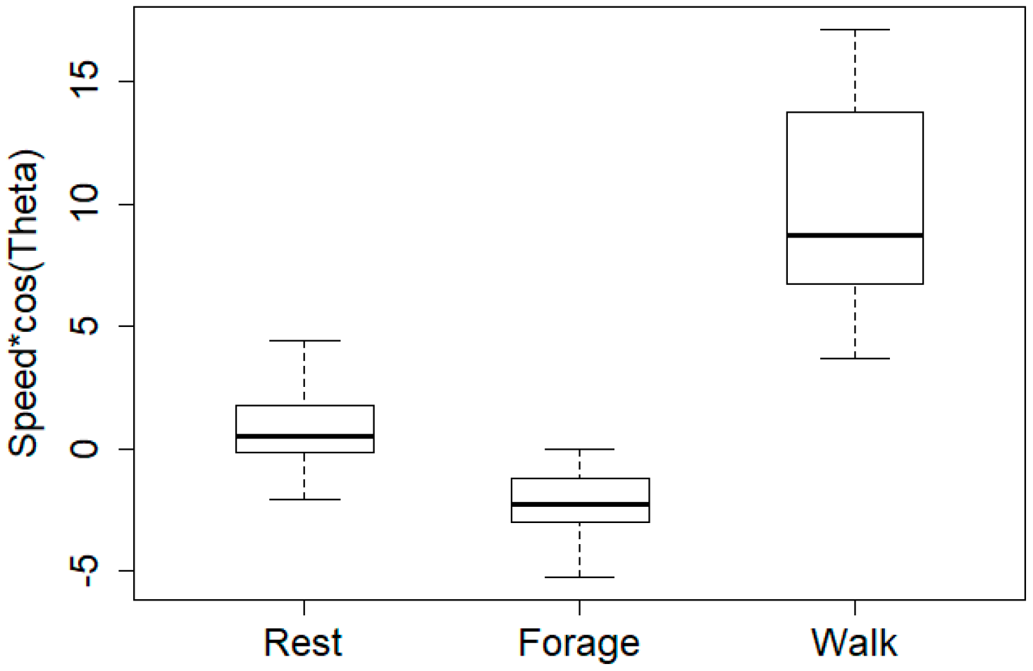
For segmenting a trajectory, we considered both “persistence velocity” and “turning velocity” when identifying behavioral change points. However, for clustering we considered only the persistence velocity values, because their associated distribution, unlike those of turning velocity, can discriminate between the three behaviors mentioned above (see Section 5, results): walking is characterized by high persistence velocity values, foraging by low values, and resting by intermediate values. Additionally, the directional histogram of turning angle values for each behavior increases our confidence to draw comparison across behaviors.
Unlike the approach in [21], for each segment we consider the overall distribution of the movement parameters (in our case, persistence velocity), rather than a specific parameter like central tendency. We use the Kolmogorov-Smirnov (ks) distance [52] to determine the distance between the segments’ persistence velocity distributions. No assumptions about the distributions are required (52). Unlike the “Pearson correlation measure” or the “cosine measure” [53], the ks-distance metric can compare vectors of different lengths. Using the R-package “adehabitat” [54], we simulated a number of trajectories based on correlated random walk (CRW) models with different characteristics [55], and figured out how well the ks-metric differentiated between the different CRW models.
Given the observed persistence velocities Vp(t1), Vp(t2), …, Vp(tn) of a particular segment containing n samples, the empirical distribution function Fn(Vp) is defined as the fraction of the observations that have values that are less than or equal to the value Vp. Thus Fn(Vp) is the empirical cumulative distribution function, with respect to the n observations of the segment [52]. The ks metric is defined on the space of distribution functions, and the ks-distance between two empirical distribution functions [52,56,57] is obtained by calculating the supremum over the set of differences. Figure 1 indicates the ks-distance between two empirical persistence velocity distribution functions for two different segments.
From the ks-metric, we generated a distance matrix to be used for the agglomerative hierarchical clustering approach using Ward’s minimum variance method [58]. The grouping of segments into distinct movement behaviors was obtained as follows: each segment was assigned to its own cluster, and then the algorithm proceeded iteratively, so that at each stage the cluster pair to be merged was the one whose merger minimized the increase in the total within-group-error sum of squares. This continued until all segments were merged into a single cluster. The associated tree-like structure obtained by the merging process is known as a dendrogram [59,60,61].
The “hclust” function in the R programming language with the “ward.D2” criterion for hierarchical clustering was used in our method. Hierarchical methods produce not a single partitioning, but a hierarchy of nested partitions, which allows the user to consider different partitions according to the desired similarity level [53]. An essential part of the cluster analysis are the interpretations of the various clusters by a human analyst to acquire their meaning and value [23]. Careful inspection of the dendrogram and the distribution (and mean) of the persistence velocity values and the turning angle values is needed to determine an appropriate number of distinct movement behaviors. The number of distinct movement behaviors in our method is a priori considered to be unknown, except for the three movement behavioral states mentioned above.
4. Case Study
The dataset investigated in this paper belongs to an ongoing project, in which the main objective is to determine the influence of grazing on biodiversity. Four individual sheep were followed during the foraging season, in an established experimental site in Valdres in Oppland county, Norway (61.06° N, 9.40° E; Figure 2 (left)). The animals were tracked with a sampling frequency of 10 s, using Canmore GT-740FL GPS units (http://www.canmore.com.tw/pdf/GT-740FL%20DataSheet_V6.1.pdf). These units have a battery capacity of approximately 24 h when sampling data using this frequency. The GPS units were equipped with extra battery capacity, which extended the capacity to 3–4 days. The GPS position accuracy is specified as 2.5 m CEP (CEP, circular error probable, which is the radius of the smallest circle centered at the true position that covers 50% of the observations) under optimal conditions. The waterproof box with the GPS unit and batteries weighed approximately 400 g, and the size of the box was 13 cm × 10 cm × 5 cm.
The animals were also equipped with a radio bell (Telespor) which was set to transmit position signals every 15 min, so that it would be easy to find the animals. Before each observation period the sheep were captured for a few minutes, wherever they were found using radio bell signals, to replace the batteries.
The usable position data for the four sheep were collected on 15, 14, 9, and 4 different days respectively, totaling up to approximately 26 days of observations. The total number of position observations was 227,050.
The Android application “observationlogger” (https://play.google.com/store/apps/details?id=com.mortensickel.obslogger), developed by Morten Sickel, with available source code on github (https://github.com/sickel/observationlogger/releases/tag/version2_0), was used to log animal behavior (grazing, walking, resting, and other behavior) when observing the sheep. The registration times from the “observationlogger” and the tracking units were set up to automatically synchronize.
“Grazing” was registered when the animal clearly was eating, and “resting” if the animal was lying down. “Walking” was registered if the walking was associated with displacements that were not part of a grazing event. Each animal was observed for a few hours per day during GPS logging. The observations were made at a distance of approximately 25–50 m, attempting to avoid any influence on the behavior of the animals.
To reduce the amount of noise due to GNSS position errors, the dataset was resampled to 1 min intervals by averaging. For our analysis, the part of the valid position recordings that had corresponding “observationlogger” recordings was used.
5. Results
We demonstrated our method using a part of the trajectory of one of the sheep in the Valdres dataset. The trajectory part contained 4960 GPS positions logged between 00:01 a.m. and 8:20 p.m. on 7 July 2016, and is shown in Figure 2 (right). The corresponding ground truth movement behavior was recorded by a human observer from 7:20 a.m. until 3:33 p.m., and classified into “foraging behavior”, ”resting behavior”, “walking behavior” and “other behavior”. The observer recorded the behaviors quite regularly, but when a specific behavior lasted for a while, observations were generally not recorded until a change in behavior took place. The model performance was assessed by comparing the predicted behaviors using our model with the ground truth (field) observations, using a confusion matrix.
By doing the BCPA for various moving window sizes and inspecting their diagnostic plots, we concluded that 30 consecutive sampling points (equivalent to considering a time interval of 30 min) was a feasible moving window size for our dataset. Figure 3 illustrates the corresponding diagnostic plots, including the qq-norm plot, the histogram, and the auto-correlation function of the standardized example dataset for persistence velocity (panel a) and turning velocity (panel b). The result is consistent with the required assumption of normality. The residual plots show that the model has captured the dominant patterns of the data quite well, although there is a small amount of autocorrelation left in the residuals (indicated by some significant spikes in the autocorrelation function plotted in the rightmost parts of Figure 3a,b).
The dendrogram resulting from the hierarchical clustering procedure (Figure 4) guides the choice of the number of clusters in the observed data. One might expect that there would be a certain number of clusters (e.g., 1, 2, or 3 for Figure 4). With reference to Figure 4, one cluster means that the whole dataset is a group, two clusters means that the leftmost (red) box is one group and the two rightmost boxes (colored blue and green) are the other group, while three clusters means that each colored box is a separate group. A subsequent analysis, based on visual inspection of the distribution of the turning angle and persistence velocity values, is recommended in order to confirm the appropriate number of clusters. The preferable number is the alternative that produces the most homogeneous clusters with respect to distinguishable persistence velocity boxplots and turning angle histograms (see Section 3.2). In other words, the behavior with the highest values for persistence velocity should have a mean turning angle value of around zero radian, with low variance to correspond to walking. The behavior with intermediate values for persistence velocity should have a mean turning angle value of around zero radian with high variance, to correspond to resting. The behavior with the lowest values for persistence velocity should have a mean turning angle value different from zero with low variance, to correspond to grazing.
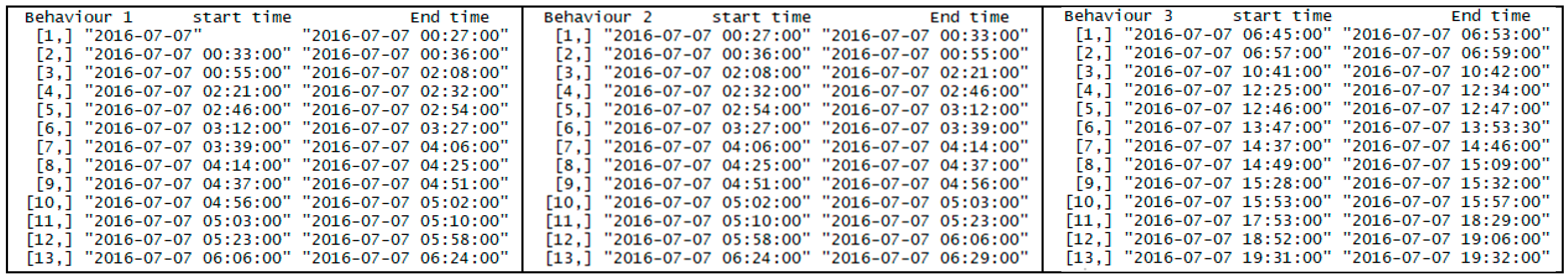
When using three clusters (corresponding to the three colored boxes in Figure 4), the textual output of our algorithm, including the start and the end times for each cluster, is shown in Figure 5.
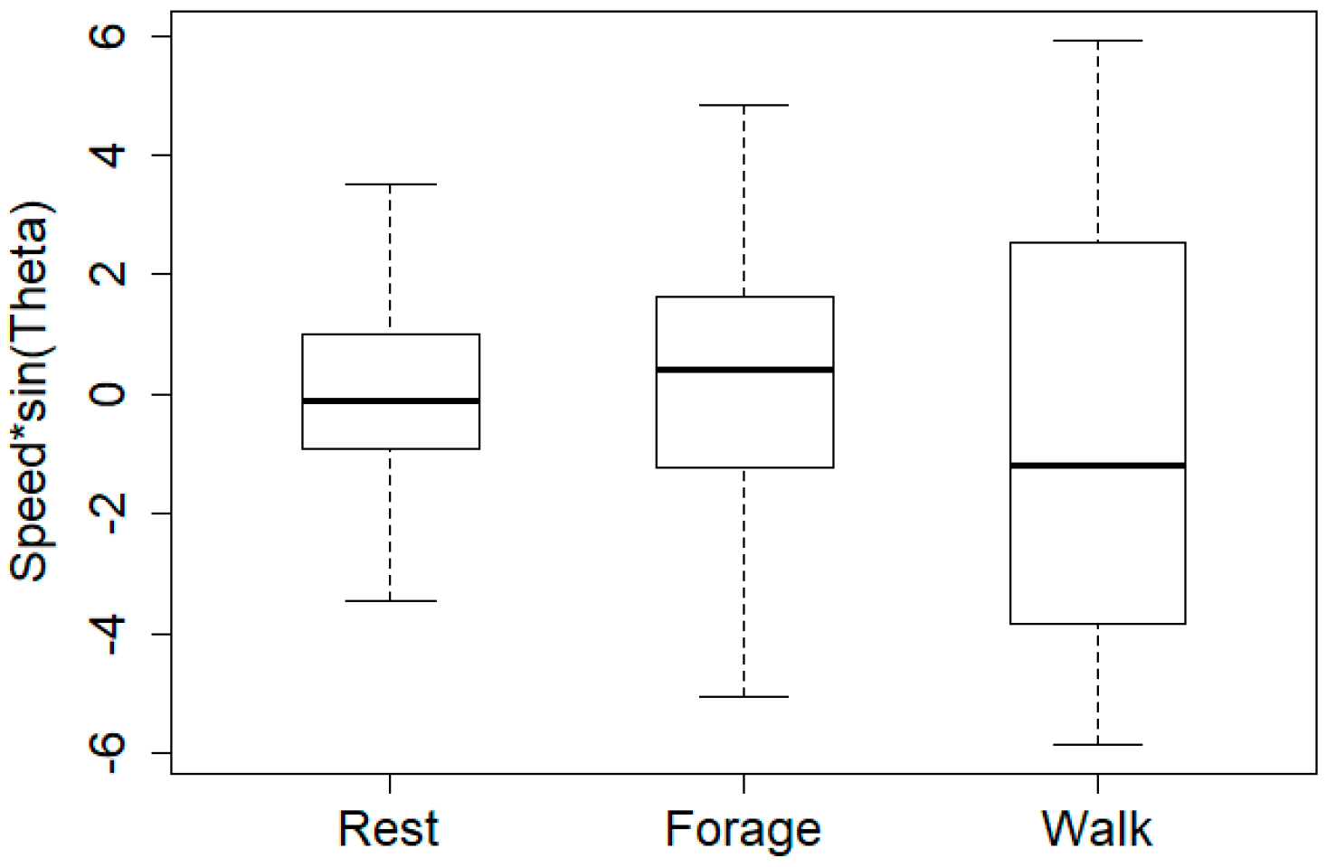
As already mentioned, for clustering we considered only the persistence velocity values, because their distribution (Figure 6), unlike the turning velocity values (Figure 7), can discriminate between the three behaviors.
The boxplots of persistence velocity values for each cluster in Figure 6, and the directional histograms summarizing the turning angle values for each cluster in Figure 8, are considered in combination, in order to assign meaningful movement behavior names to the clusters.
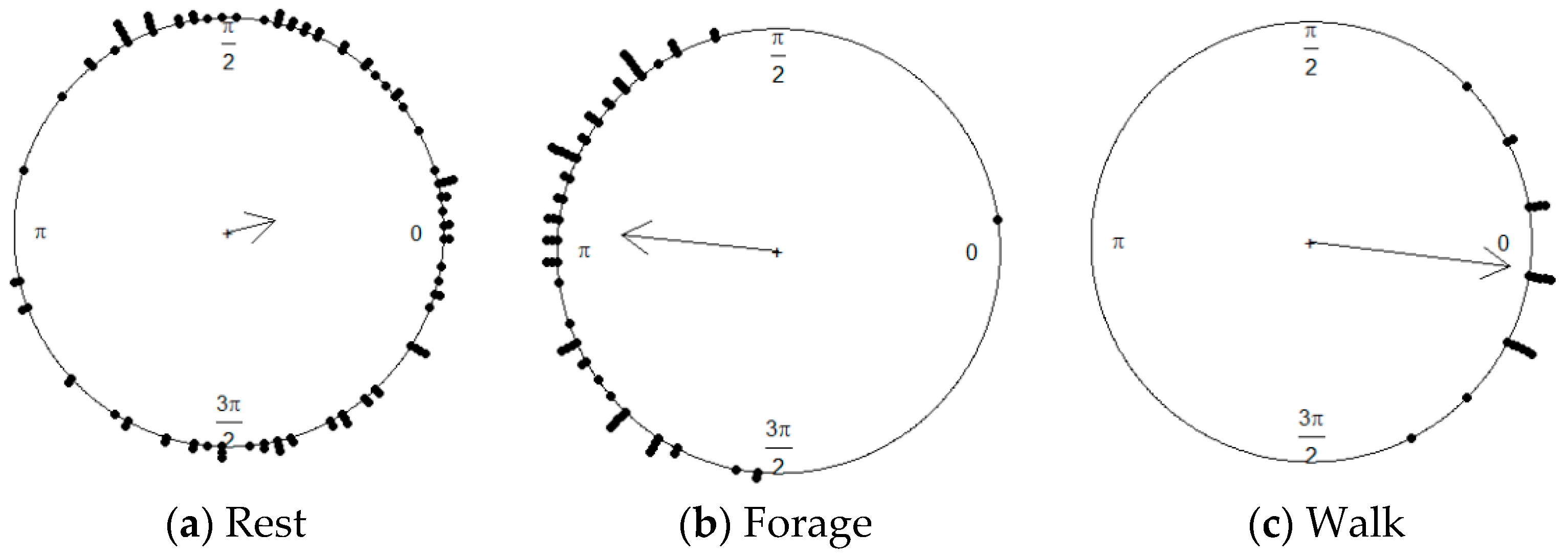
Figure 8c shows a movement behavior where most turning angles are small, suggesting that the overall direction is persistent. A comparison with the corresponding boxplot of persistence velocity values in Figure 6 (Walk) suggests that the particular movement behavior is consistent with walking.
Figure 8a shows a movement behavior in which the mean of the turning angles is close to zero with a directional persistence of around zero. A comparison with the corresponding boxplot of persistence velocity values in Figure 6 (Rest), suggests that the particular movement behavior is consistent with resting. By similar reasoning and visual inspection of Figure 6 (Forage) and Figure 8b, we can conclude that the remaining movement behavior is consistent with foraging behavior. The latter observations are characterized by low ‘Persistence velocity’ values and an overall mean direction vector with a non-zero angle, i.e., a sinuous type of motion, indicating a tendency to reverse direction.
By comparing the derived movement behaviors to the ground truth movement behavior recorded by a human observer, we obtain a validation of the resulting model in terms of its discriminative power between behavioral states. The model performance is presented by a confusion matrix (Table 1) that shows how the number of minutes for each type of observed behavior is distributed according to the predictions of our model. Each row in the confusion matrix represents an observed movement behavior, while each column represents a particular movement behavior predicted by our model. Hence, each cell counts the number of minutes in the intersection of these two observed and predicted movement behaviors. The diagonal entries of the confusion matrix represent the correct predictions, and off-diagonal values represent the misclassifications. The sum of values on the diagonal divided by the sum of all the matrix values shows the accuracy. Thus, using the demonstration data, the accuracy obtained from the confusion matrix in Table 1 is 77%. Analysis of seven GPS recording days where corresponding “observationlogger” data are available indicates an averaged accuracy for our dataset of 80.75% ± 5.9% (SE). For these seven days, the number of hours of corresponding “observationlogger” data varied from 2 h to 8 h, with an average of 4.6 h. The total number of valid GPS points was 39,123.
6. Concluding Remarks
With this paper, our goal has been to identify activity patterns of individual animals over a 24 h time span. We demonstrate how changes in movement behavior can be inferred from the tracks of individual animals, and how the movement behavior of individual animals varies over time. The method for discriminating between different animal behaviors described in this paper requires no specialist coding experience or statistical background. The source code is provided as a Supplementary File.
In contrast to other methods proposed for the same purpose, our method requires neither a temporal regularization of the data nor a strict a priori value for the number of movement behavioral states, nor the specification of the movement model. The proposed method is exploratory and depends only on location in space and time, with no need for ancillary data like accelerator sensor values. The heuristics described for choosing the moving window size (see Section 3.1.1) and the number of clusters (see Section 5) seem difficult to replace by completely objective criteria. Validation of the selection procedure by using the proposed diagnostic plots (Figure 3), box plots (Figure 6), and histograms (Figure 8) is therefore urgent for our confidence in the goodness of these values.
Consideration of the diurnal activity pattern for individual sheep over several days should improve the possibilities of detecting deviant movement behavior for individual animals. Some cautionary steps are, however, required before applying our method to large datasets. It is well-known from the literature that applying hierarchical clustering to large datasets is challenging, but some advanced and efficient alternatives do exist (e.g., [62]). An alternative is running the hierarchical clustering on a manageable subset of the included animals. The mean/overall distribution for each of the (k) resulting clusters can then be used to initialize a k-means clustering process (using the ks-metric) to cluster the complete dataset into k clusters.
In spite of its accuracy, being sensitive to the uncertainty in the location data and the derived movement parameters, we claim that our method for identifying movement behavioral states from tracking data has proven successful in practice. There are, however, uncertainties associated with the identification and recording of activities during field observations. In addition, the matching of field observations and tracking data must be executed carefully, to prevent loss of accuracy in the resulting models. Further work is required to address these issues in the best possible way.
Supplementary Materials
The following are available online at https://www.mdpi.com/2220-9964/7/2/78/s1. Source code S1 in the R programming language: ‘manuscript-supplementary.R’.
Acknowledgements
We want to thank the farmer for his inspiring cooperation and valuable help regarding use of his animals and help to change GPS collars during the fieldwork period. We would also like to thank Morten Sickel for facilitating data collection and making the data collected available for the analyses in this paper, and colleagues in NIBIO for conscientious collection of observation data. We are very thankful to The Norwegian Agriculture Agency, which was the main financier of the project that provided data to this work. This research was supported by the Norwegian University of Life Sciences under project number 1301051701.
Author Contributions
H.S. designed, performed the field experiments. M.T. developed the theoretical framework, did the programming task and drafted the manuscript. H.T. and U.G.I assisted in writing the manuscript. H.T. supervised the findings of this work and was in charge of overall direction and coordination between all authors.
Conflicts of Interest
The authors declare no conflict of interest.
References
- Cooke, S.J.; Hinch, S.G.; Wikelski, M.; Andrews, R.D.; Kuchel, L.J.; Wolcott, T.G.; Butler, P.J. Biotelemetry: A mechanistic approach to ecology. Trends Ecol. Evol. 2004, 19, 334–343. [Google Scholar] [CrossRef] [PubMed]
- Dray, S.; Royer-Carenzi, M.; Calenge, C. The exploratory analysis of autocorrelation in animal-movement studies. Ecol. Res. 2010, 25, 673–681. [Google Scholar] [CrossRef]
- Morales, J.M.; Haydon, D.T.; Frair, J.; Holsinger, K.E.; Fryxell, J.M. Extracting more out of relocation data: Building movement models as mixtures of random walks. Ecology 2004, 85, 2436–2445. [Google Scholar] [CrossRef]
- Edelhoff, H.; Signer, J.; Balkenhol, N. Path segmentation for beginners: An overview of current methods for detecting changes in animal movement patterns. Mov. Ecol. 2016, 4, 21. [Google Scholar] [CrossRef] [PubMed]
- Patterson, T.A.; Thomas, L.; Wilcox, C.; Ovaskainen, O.; Matthiopoulos, J. State-space models of individual animal movement. Trends Ecol. Evol. 2008, 23, 87–94. [Google Scholar] [CrossRef] [PubMed]
- Dodge, S.; Weibel, R.; Lautensch, A.-K. Towards a taxonomy of movement patterns. Inf. Vis. 2008, 7, 240–252. [Google Scholar] [CrossRef] [Green Version]
- Guo, Y.; Poulton, G.; Corke, P.; Bishop-Hurley, G.J.; Wark, T.; Swain, D.L. Using accelerometer, high sample rate GPS and magnetometer data to develop a cattle movement and behaviour model. Ecol. Model. 2009, 220, 2068–2075. [Google Scholar] [CrossRef] [Green Version]
- de Weerd, N.; van Langevelde, F.; van Oeveren, H.; Nolet, B.A.; Kölzsch, A.; Prins, H.H.; de Boer, W.F. Deriving animal behaviour from high-frequency GPS: Tracking cows in open and forested habitat. PLoS ONE 2015, 10, e0129030. [Google Scholar] [CrossRef] [PubMed]
- Gurarie, E.; Andrews, R.D.; Laidre, K.L. A novel method for identifying behavioural changes in animal movement data. Ecol. Lett. 2009, 12, 395–408. [Google Scholar] [CrossRef] [PubMed]
- Han, J.; Lee, J.-G.; Kamber, M. An overview of clustering methods in geographic data analysis. In Geographic Data Mining and Knowledge Discovery, 2nd ed.; Miller, H.J., Han, J., Eds.; CRC Press: Boca Raton, FL, USA, 2009; pp. 149–187. [Google Scholar]
- Schick, R.S.; Loarie, S.R.; Colchero, F.; Best, B.D.; Boustany, A.; Conde, D.A.; Halpin, P.N.; Joppa, L.N.; McClellan, C.M.; Clark, J.S. Understanding movement data and movement processes: Current and emerging directions. Ecol. Lett. 2008, 11, 1338–1350. [Google Scholar] [CrossRef] [PubMed]
- Gurarie, E.; Bracis, C.; Delgado, M.; Meckley, T.D.; Kojola, I.; Wagner, C.M. What is the animal doing? Tools for exploring behavioural structure in animal movements. J. Anim. Ecol. 2016, 85, 69–84. [Google Scholar] [CrossRef] [PubMed]
- Demšar, U.; Buchin, K.; Cagnacci, F.; Safi, K.; Speckmann, B.; Van de Weghe, N.; Weiskopf, D.; Weibel, R. Analysis and visualisation of movement: An interdisciplinary review. Mov. Ecol. 2015, 3, 5. [Google Scholar] [CrossRef] [PubMed] [Green Version]
- Postlethwaite, C.M.; Brown, P.; Dennis, T.E. A new multi-scale measure for analysing animal movement data. J. Theor. Biol. 2013, 317, 175–185. [Google Scholar] [CrossRef] [PubMed]
- Schwager, M.; Anderson, D.M.; Butler, Z.; Rus, D. Robust classification of animal tracking data. Comput. Electron. Agric. 2007, 56, 46–59. [Google Scholar] [CrossRef]
- Jonsen, I.D.; Flemming, J.M.; Myers, R.A. Robust state-space modeling of animal movement data. Ecology 2005, 86, 2874–2880. [Google Scholar] [CrossRef]
- Gutenkunst, R.; Newlands, N.; Lutcavage, M.; Edelstein-Keshet, L. Inferring resource distributions from Atlantic bluefin tuna movements: An analysis based on net displacement and length of track. J. Theor. Biol. 2007, 245, 243–257. [Google Scholar] [CrossRef] [PubMed]
- Fauchald, P.; Tveraa, T. Using first-passage time in the analysis of area-restricted search and habitat selection. Ecology 2003, 84, 282–288. [Google Scholar] [CrossRef]
- Tremblay, Y.; Roberts, A.J.; Costa, D.P. Fractal landscape method: An alternative approach to measuring area-restricted searching behavior. J. Exp. Biol. 2007, 210, 935–945. [Google Scholar] [CrossRef] [PubMed] [Green Version]
- Jonsen, I.D.; Myers, R.A.; Flemming, J.M. Meta-analysis of animal movement using state-space models. Ecology 2003, 84, 3055–3063. [Google Scholar] [CrossRef]
- Zhang, J.; O’Reilly, K.M.; Perry, G.L.W.; Taylor, G.A.; Dennis, T.E. Extending the Functionality of Behavioural Change-Point Analysis with k-Means Clustering: A Case Study with the Little Penguin (Eudyptula minor). PLoS ONE 2015, 10, e0122811. [Google Scholar] [CrossRef] [PubMed]
- Lavielle, M. Detection of multiple changes in a sequence of dependent variables. Stoch. Process. Their Appl. 1999, 83, 79–102. [Google Scholar] [CrossRef]
- Rinzivillo, S.; Pedreschi, D.; Nanni, M.; Giannotti, F.; Andrienko, N.; Andrienko, G. Visually driven analysis of movement data by progressive clustering. Inf. Vis. 2008, 7, 225–239. [Google Scholar] [CrossRef]
- Lee, J.-G.; Han, J.; Whang, K.-Y. Trajectory clustering: A partition-and-group framework. In Proceedings of the 2007 ACM SIGMOD International Conference on Management of Data, Beijing, China, 11–14 June 2007; ACM: New York, NY, USA, 2007; pp. 593–604. [Google Scholar]
- Miller, H.J.; Han, J. Geographic Data Mining and Knowledge Discovery, 2nd ed.; CRC Press: Boca Raton, FL, USA, 2009. [Google Scholar]
- Etienne, L.; Devogele, T.; Bouju, A. Spatio-temporal trajectory analysis of mobile objects following the same itinerary. Adv. Geo-Spat. Inf. Sci. 2012, 10, 47–57. [Google Scholar]
- Nanni, M.; Pedreschi, D. Time-focused clustering of trajectories of moving objects. J. Intell. Inf. Syst. 2006, 27, 267–289. [Google Scholar] [CrossRef]
- Dodge, S.; Laube, P.; Weibel, R. Movement similarity assessment using symbolic representation of trajectories. Int. J. Geogr. Inf. Sci. 2012, 26, 1563–1588. [Google Scholar] [CrossRef] [Green Version]
- Yanagisawa, Y.; Akahani, J.-I.; Satoh, T. Shape-Based Similarity Query for Trajectory of Mobile Objects. In Proceedings of the 4th International Conference on Mobile Data Management, Melbourne, Australia, 21–24 January 2003; Chen, M.-S., Chrysanthis, P.K., Sloman, M., Zaslavsky, A., Eds.; Springer: Berlin/Heidelberg, Germany, 2003; pp. 63–77. [Google Scholar]
- Vlachos, M.; Gunopulos, D.; Das, G. Rotation invariant distance measures for trajectories. In Proceedings of the Tenth ACM SIGKDD International Conference on Knowledge Discovery and Data Mining, Seattle, WA, USA, 22–25 August 2004; ACM: New York, NY, USA, 2004; pp. 707–712. [Google Scholar]
- Chen, L.; Özsu, M.T.; Oria, V. Robust and fast similarity search for moving object trajectories. In Proceedings of the 2005 ACM SIGMOD International Conference on Management of Data, Baltimore, Maryland, 14–16 June 2005; ACM: New York, NY, USA, 2005; pp. 491–502. [Google Scholar]
- Vlachos, M.; Gunopoulos, D.; Kollios, G. Discovering Similar Multidimensional Trajectories. In Proceedings of the 18th International Conference on Data Engineering, San Jose, CA, USA, 26 February–1 March 2002; p. 673. [Google Scholar]
- Alt, H.; Guibas, L.J. Discrete geometric shapes: Matching, interpolation, and approximation. Handb. Comput. Geom. 1999, 1, 121–153. [Google Scholar]
- Alt, H.; Godau, M. Computing the Fréchet distance between two polygonal curves. Int. J. Comput. Geom. Appl. 1995, 5, 75–91. [Google Scholar] [CrossRef]
- Andrienko, G.; Andrienko, N.; Wrobel, S. Visual analytics tools for analysis of movement data. ACM SIGKDD Explor. Newsl. 2007, 9, 38–46. [Google Scholar] [CrossRef]
- Pelekis, N.; Andrienko, G.; Andrienko, N.; Kopanakis, I.; Marketos, G.; Theodoridis, Y. Visually exploring movement data via similarity-based analysis. J. Intell. Inf. Syst. 2012, 38, 343–391. [Google Scholar] [CrossRef]
- Thiebault, A.; Tremblay, Y. Splitting animal trajectories into fine-scale behaviorally consistent movement units: Breaking points relate to external stimuli in a foraging seabird. Behav. Ecol. Sociobiol. 2013, 67, 1013–1026. [Google Scholar] [CrossRef]
- Cagnacci, F.; Boitani, L.; Powell, R.A.; Boyce, M.S. Animal ecology meets GPS-based radiotelemetry: A perfect storm of opportunities and challenges. R. Soc. 2010. [Google Scholar] [CrossRef] [PubMed]
- Schwarz, G. Estimating the dimension of a model. Ann. Stat. 1978, 6, 461–464. [Google Scholar] [CrossRef]
- Gurarie, E. Behavioral Change Point Analysis in R: The bcpa package (R package version 1.1). Available online: https://pdfs.semanticscholar.org/dc3e/3c9baac39d228f1dd2de4b35431395c76fd3.pdf (accessed on 22 February 2018).
- Calenge, C.; Dray, S.; Royer-Carenzi, M. The concept of animals’ trajectories from a data analysis perspective. Ecol. Inf. 2009, 4, 34–41. [Google Scholar] [CrossRef]
- Benhamou, S. How to reliably estimate the tortuosity of an animal’s path: Straightness, sinuosity, or fractal dimension? J. Theor. Biol. 2004, 229, 209–220. [Google Scholar] [CrossRef] [PubMed]
- Laube, P.; Purves, R.S. How fast is a cow? Cross-scale analysis of movement data. Trans. GIS 2011, 15, 401–418. [Google Scholar] [CrossRef]
- Murtagh, F. A survey of recent advances in hierarchical clustering algorithms. Comput. J. 1983, 26, 354–359. [Google Scholar] [CrossRef]
- Berkhin, P. A survey of clustering data mining techniques. Group. Multidimens. Data 2006, 25, 71. [Google Scholar]
- Van Moorter, B.; Visscher, D.R.; Jerde, C.L.; Frair, J.L.; Merrill, E.H. Identifying movement states from location data using cluster analysis. J. Wildl. Manag. 2010, 74, 588–594. [Google Scholar] [CrossRef]
- Garriga, J.; Palmer, J.R.; Oltra, A.; Bartumeus, F. Expectation-maximization binary clustering for behavioural annotation. PLoS ONE 2016, 11, e0151984. [Google Scholar] [CrossRef] [PubMed] [Green Version]
- Braun, E.; Geurten, B.; Egelhaaf, M. Identifying prototypical components in behaviour using clustering algorithms. PLoS ONE 2010, 5, e9361. [Google Scholar] [CrossRef] [PubMed]
- Hurford, A. GPS measurement error gives rise to spurious 180 turning angles and strong directional biases in animal movement data. PLoS ONE 2009, 4, e5632. [Google Scholar] [CrossRef] [PubMed]
- Pewsey, A.; Neuhäuser, M.; Ruxton, G.D. Circular Statistics in R; Oxford University Press: Oxford, UK, 2013. [Google Scholar]
- Jammalamadaka, S.R.; Sengupta, A. Topics in Circular Statistics; World Scientific: Singapore, 2001. [Google Scholar]
- Rachev, S.T.; Klebanov, L.B.; Stoyanov, S.V.; Fabozzi, F.J. Probability distances and probability metrics: Definitions. In The Methods of Distances in the Theory of Probability and Statistics; Springer: Cham, Switzerland, 2013; pp. 11–31. [Google Scholar]
- Rokach, L. A survey of clustering algorithms. In Data Mining and Knowledge Discovery Handbook; Maimon, O., Rokach, L., Eds.; Springer: New York, NY, USA, 2010; pp. 269–298. [Google Scholar]
- Calenge, C. The package “adehabitat” for the R software: A tool for the analysis of space and habitat use by animals. Ecol. Model. 2006, 197, 516–519. [Google Scholar] [CrossRef]
- Kareiva, P.; Shigesada, N. Analyzing insect movement as a correlated random walk. Oecologia 1983, 56, 234–238. [Google Scholar] [CrossRef] [PubMed]
- Deza, M.M.; Deza, E. Encyclopedia of distances. In Encyclopedia of Distances; Springer: Cham, Switzerland, 2009; pp. 1–583. [Google Scholar]
- Gibbs, A.L.; Su, F.E. On choosing and bounding probability metrics. Int. Stat. Rev. 2002, 70, 419–435. [Google Scholar] [CrossRef]
- Murtagh, F.; Legendre, P. Ward’s hierarchical agglomerative clustering method: Which algorithms implement ward’s criterion? J. Classif. 2014, 31, 274–295. [Google Scholar] [CrossRef]
- Bridges, C.C., Jr. Hierarchical cluster analysis. Psychol. Rep. 1966, 18, 851–854. [Google Scholar] [CrossRef]
- Xu, R.; Wunsch, D. Survey of clustering algorithms. IEEE Trans. Neural Netw. 2005, 16, 645–678. [Google Scholar] [CrossRef] [PubMed]
- Köhn, H.-F.; Hubert, L.J. Hierarchical Cluster Analysis. In Wiley StatsRef: Statistics Reference Online; John Wiley & Sons, Ltd.: Hoboken, NJ, USA, 2014. [Google Scholar]
- Vijaya, P.; Murty, M.N.; Subramanian, D. Leaders—Subleaders: An efficient hierarchical clustering algorithm for large data sets. Pattern Recognit. Lett. 2004, 25, 505–513. [Google Scholar] [CrossRef]
Figure 1.
Illustration of Kolmogorov-Smirnov (ks)-metric on the two empirical distribution functions of two different segments’ persistence velocity (red and blue lines). The dashed line shows the ks-distance between two segments’ persistence velocities.
Figure 1.
Illustration of Kolmogorov-Smirnov (ks)-metric on the two empirical distribution functions of two different segments’ persistence velocity (red and blue lines). The dashed line shows the ks-distance between two segments’ persistence velocities.

Figure 2.
Map of Norway (source: Norwegian Mapping Authority; projection: UTM 33N) with the location of the experimental site (left) and an example trajectory for one sheep over one day (right).
Figure 2.
Map of Norway (source: Norwegian Mapping Authority; projection: UTM 33N) with the location of the experimental site (left) and an example trajectory for one sheep over one day (right).

Figure 3.
Diagnostic Plots for residuals for “persistence velocity” (a) and “turning velocity” (b).

Figure 4.
Dendrogram representation of the clustered sub-trajectories; the numbers in the bottom of the plot represent the segment numbers from the trajectory segmentation.
Figure 4.
Dendrogram representation of the clustered sub-trajectories; the numbers in the bottom of the plot represent the segment numbers from the trajectory segmentation.

Figure 5.
A part of the typical text output of the algorithm (behavior 1 is resting, behavior 2 is foraging, and behavior 3 is walking).
Figure 5.
A part of the typical text output of the algorithm (behavior 1 is resting, behavior 2 is foraging, and behavior 3 is walking).

Figure 6.
Boxplot representation of persistence velocity values for each cluster. There is a significant difference between the persistence velocity values, according to the Kruskal-Wallis rank sum test (chi-square distribution with 2 degrees of freedom (X2(2) = 58.22, p < 0.01).
Figure 6.
Boxplot representation of persistence velocity values for each cluster. There is a significant difference between the persistence velocity values, according to the Kruskal-Wallis rank sum test (chi-square distribution with 2 degrees of freedom (X2(2) = 58.22, p < 0.01).

Figure 7.
Boxplot representation of turning velocity values for each cluster. There is no significant difference between the turning velocity values, according to the Kruskal-Wallis rank sum test (chi-square distribution with 2 degrees of freedom (X2(2) = 4.29, p = 0.12).
Figure 7.
Boxplot representation of turning velocity values for each cluster. There is no significant difference between the turning velocity values, according to the Kruskal-Wallis rank sum test (chi-square distribution with 2 degrees of freedom (X2(2) = 4.29, p = 0.12).

Figure 8.
Distribution of turning angles for each detected movement behavior; each dot on the perimeter of the circles represent the mean of the turning angles for one segment. The mean value of the turning angles for foraging behavior (b) tends to be near pi radians, meaning sinuous segments. While the mean value of turning angles for resting (a) and walking (c) movement behaviors tends to zero, with high variance and low variance, respectively (inverse relationship with the arrow length).


Table 1.
Confusion matrix showing the performance of the clustering. Precision = True Positives/(True Positives + False Positives). Precision (Forage) = 87.6%, Precision (Rest) = 68.7%, Precision (Walk) = 70%.
Table 1.
Confusion matrix showing the performance of the clustering. Precision = True Positives/(True Positives + False Positives). Precision (Forage) = 87.6%, Precision (Rest) = 68.7%, Precision (Walk) = 70%.
| Predicted | Forage | Rest | Walk | |
|---|---|---|---|---|
| Real | ||||
| Forage | 184 (min) | 73 (min) | 15 (min) | |
| Rest | 26 (min) | 160 (min) | 0 | |
| Walk | 0 | 0 | 35 (min) | |
© 2018 by the authors. Licensee MDPI, Basel, Switzerland. This article is an open access article distributed under the terms and conditions of the Creative Commons Attribution (CC BY) license (http://creativecommons.org/licenses/by/4.0/).
Share and Cite
MDPI and ACS Style
Teimouri, M.; Indahl, U.G.; Sickel, H.; Tveite, H. Deriving Animal Movement Behaviors Using Movement Parameters Extracted from Location Data. ISPRS Int. J. Geo-Inf. 2018, 7, 78. https://doi.org/10.3390/ijgi7020078
AMA Style
Teimouri M, Indahl UG, Sickel H, Tveite H. Deriving Animal Movement Behaviors Using Movement Parameters Extracted from Location Data. ISPRS International Journal of Geo-Information. 2018; 7(2):78. https://doi.org/10.3390/ijgi7020078
Chicago/Turabian StyleTeimouri, Maryam, Ulf Geir Indahl, Hanne Sickel, and Håvard Tveite. 2018. "Deriving Animal Movement Behaviors Using Movement Parameters Extracted from Location Data" ISPRS International Journal of Geo-Information 7, no. 2: 78. https://doi.org/10.3390/ijgi7020078
Note that from the first issue of 2016, this journal uses article numbers instead of page numbers. See further details here.