
Analyzing the Behaviors of OpenStreetMap Volunteers in Mapping Building Polygons Using a Machine Learning Approach


Department of Geomatic Engineering, Yildiz Technical University, Istanbul 34220, Turkey
ISPRS Int. J. Geo-Inf. 2022, 11(1), 70; https://doi.org/10.3390/ijgi11010070
Submission received: 29 November 2021
/
Revised: 1 January 2022
/
Accepted: 12 January 2022
/
Published: 17 January 2022
(This article belongs to the Special Issue Cartographic Communication of Big Data)
Abstract
:Mapping as an action in volunteered geographic information is complex in light of the human diversity within the volunteer community. There is no integrated solution that models and fixes all data heterogeneity. Instead, researchers are attempting to assess and understand crowdsourced data. Approaches based on statistics are helpful to comprehend trends in crowd-drawing behaviors. This study examines trends in contributors’ first decisions when drawing OpenStreetMap (OSM) buildings. The proposed approach evaluates how important the properties of a point are in determining the first point of building drawings. It classifies the adjacency types of the buildings using a random forest classifier for the properties and aids in inferring drawing trends from the relative impact of each property. To test the approach, detached and attached building groups in Istanbul and Izmir, Turkey, were used. The result had an 83% F-score. In summary, the volunteers tended to choose as first points those further away from the street and building centroid and provided lower point density in the detached buildings than the attached ones. This means that OSM volunteers paid more attention to open spaces when drawing the first points of the detached buildings in the study areas. The study reveals common drawing trends in building-mapping actions.
1. Introduction
Twenty years ago, if asked what the most popular aspect of geographic information studies was, many people would have answered, ‘the increasing use of geographic information systems’ (GIS). Now, similarly, volunteered geographic information impels the geoinformation society to comprehend geospatial datasets created by volunteers. Crowdsourced platforms involving spatial data generation by volunteer participants are called volunteered geographical information (VGI) projects. Each of the independent volunteers has an equal right to generate spatial data and update existing data. In other words, volunteer participants have the facility to provide unlimited geographic data and to edit each other’s contributions. However, there is no requirement for cartographic qualifications among participants in VGI platforms. Therefore, there is always a possibility that one can be a non-expert cartographer. Volunteers whose expertise is not confirmed as sufficient can create geographic data through online interfaces [1,2]. Spatial data consistency is achieved only after any detected conflicts have been resolved manually [3]. Therefore, various scientific studies have been carried out to determine whether or not the geographic data generated through VGI can be used for professional purposes, like other maps produced by cartographers. Most studies have focused on evaluating the accuracy and completeness of semantic and geometric data in VGI. Only a few studies have directly investigated volunteers’ behavior [4,5,6,7,8]. Briefly, they examined the geometric and semantic contributions and assessed the activities of volunteers.
This section firstly gives a general introduction to OpenStreetMap, the most popular VGI platform. Secondly, the quality assessment studies of VGI data are summarized, as they are one of the most common research interests on VGI data. Then, previous studies that shape the motivation of this paper and the scope of the investigation of contributors’ behavior are presented. Finally, the motivation and a brief outline of the study are introduced.
OSM, Wheelmap, Wikimapia, and WorldMap are some of the significant VGI projects. The Wheelmap project is carried out for individuals with walking disabilities to identify geographical objects on the map suitable for wheelchair use [9]. WorldMap is a project that rapidly initiated the generation of geographic data for Africa [10], before expanding to other continents. The Wikimapia project was established in 2006 [11] with the aim of creating a geographic data encyclopedia inspired by Wikipedia. One of the pioneering VGI projects is OSM. It is used for all geographical entities that are predominantly located close to or related to roads; however, there is no limit on geographic data diversity in the project [12]. Participants can freely contribute geometric and semantic information for any location in the world. Data are made available weekly at planet.osm. At the beginning of the OSM project, while some of the participants were active, many of them only became members, abstaining from any editing. Neis and Zipf [13] mentioned that only 38% of the volunteers made at least one contribution, and just 5% actively contributed as OSM volunteers in real terms. Over the years, with the increase in member participation, the compressed version of the planet data available for sharing on 31 December 2020 has grown to 54.5 GB and the extracted version in XML format, 1338.4 GB [14]. There is no geometric, semantic, or cartographic internal control mechanism except the authority of volunteers to regulate each other’s contributions, and there are no restrictive rules that enable the evaluation of this large geographic data source. Therefore, Mooney and Corcoran [5] remark that it is necessary for users to evaluate the quality of the OSM data, especially for map applications that require high geometric accuracy and precision. Basiri et al. [15] mentioned the problems of OSM contributions as arising from volunteers’ lack of GIS experience, insufficient knowledge of the area contributed, interpretations of similar attributes with different tags for the same objects, and additions of different numbers of tags to similar objects.
Early studies to evaluate OSM data focused on determining accuracy and completeness using reference data. Haklay [16] focused on a quality analysis based on comparing the UK’s OSM data with large-scale data produced by Ordnance Survey. The author determined that the OSM geometric data accuracy is approximately 6 m. In France, Girres and Touya [17] used evaluation measures for OSM data that determine spatial data quality, such as geometric, attribute, semantic and temporal accuracy, logical consistency, and completeness. Mondzech and Sester [18] evaluated OSM quality in terms of pedestrian navigation by comparing ATKIS and OSM data. They analyzed some cities in Germany and determined that the datasets where long routes were formed consisted of incomplete data. Da Costa [19] evaluated the completeness of OSM buildings by comparing them with official building datasets. The study showed that completeness was relatively high in town centers but decreased further away from urban areas. Zhang and Malczewski [20] evaluated the quality of OSM road data in Canada. As a result of their analysis using spatial data evaluation measures such as completeness, spatial, attribute, and semantic accuracy, they found that there was more participation in urban road networks than in rural areas. Mobasheri et al. [21] conducted an initial assessment of sidewalk data in OSM to increase the awareness and engagement of the crowd for enriching sidewalk information in different European cities. In Iran, Mohammadi and Sedaghat [22] proposed a framework to estimate VGI quality using an index to classify them based on the users’ needs by using an integrated approach consisting of a matching process and a neural network classifier.
Reference data can provide information on whether geometric or semantic data is correct, but it does not provide information on volunteers’ choice of tag type or general drawing trends [5]. Studies without reference data generally assess OSM objects with the help of geometric and semantic measures and make inferences about the evolution of data or the behavior of contributors. Some of the studies conducted without reference data have been focused on the evolution and automated generation of OSM data. Corcoran et al. [23] analyzed the temporal evolution of three OSM road networks in Ireland. They evaluated the results by densification and exploration in urban areas. Zhao et al. [24] examined the evolution of Beijing’s OSM road networks between 2009 and 2012 in terms of geometric, topological, and centrality measures; in the study area, it was determined that OSM volunteers started to contribute from the city boundaries and that their drawings were directed towards the city center. Hacar et al. [25] examined the evolution of the OSM road networks in Ankara between 2007 and 2017 by using centrality measures. They measured the temporal completeness parameter, the sinuosity of the roads, and the activation density of volunteers over the years. It was observed that as the experience of contributors increased, they made more detailed contributions. Basiri et al. [26] analyzed trajectories of movement to extract some patterns and rules, which help to detect anomalies and errors within OSM data. In addition, Basiri et al. [15] conducted a study with the assumption that some characteristics of raw trajectory data may be related to the geometry and attributes of the objects. They proposed an approach to generating new objects or editing existing data by using data mining techniques, which include cartographic generalization, and matching steps. Hacar [27] suggested a semi-automated approach to identify the values of leisure tags. The approach uses geometric (rectangularity, density, area, and distances to bus stop and shop) and semantic (amenity) data and estimates the key values using a random forest classifier.
Creating geographical objects and converting them into map features is the specialty of cartographers. As in many engineering branches, this field requires extensive knowledge of analytical geometry. There are many cartographic rules that are defined by graphic and geometric resolution limits during the creation of drawings. Moreover, when the act of drawing is considered an artistic activity, it can be recognized that subjective actions are also performed [28]. These actions are habits shaped by the experience of cartographers over time, and there are no specific common standards. For example, there is no objective rule for determining where to start drawing a road network, forest border, lake, or building. It may not be meaningful to scientifically investigate the subjective drawing habits of cartographers in projects consisting of several cartographers. However, volunteers contributing to crowdsourced VGI data should be considered outside this scope. In VGI projects, unlike others, it is necessary to talk about the behavior of hundreds of thousands of people, rather than individual habits. Scientific research on crowdsourced contribution behavior has been conducted using both geometric and semantic approaches. Mooney et al. [4] evaluated the quality of OSM data by examining the creation of polygons representing hydrography and forested areas. They stated that it was easier for the volunteers to draw hydrographic features and boundaries from satellite images than to draw the boundaries of the forest area.
However, most of the quality assessment studies of OSM were designed to evaluate the semantic tags and their values. Mooney and Corcoran [5,29] examined frequently updated data (at least 15 times) by country. Although frequently changed objects have certain common points, it was observed that they did not have a correlation. They found that more than 90% of the OSM data changed less than three times and there was no strong relationship between the number of contributors and the number of tags. Jilani et al. [6] developed a machine learning (ML) model to predict the “highway = *” tag values that refer to OSM road classes. They took some of the relatively reliable London OSM road data as a reference. As a result of the experiment, while more than 50% of residential, pedestrian, primary, motorway, primarylink, and motorwaylink were predicted correctly, less than 40% of the cycleway, bridleway, path, secondary, and secondarylink were correct. Due to the density of data in urban areas, the use of the ‘Map Features’ guide on the OSM Wiki website helps to make more careful and accurate contributions [30]. In the manual, tag names that are especially preferred and accepted by users over several years are listed with their definitions. Contributors can select tags suitable for a characteristic of a geographic object from the list and enter data compatible with other users. Davidovic et al. [7] investigated how often OSM volunteers in 30 different urban areas took the OSM Wiki web page into consideration. They found that the volunteers were in general agreement with the guideline on the ‘Map Features’ page, but that the same types of geographic objects were created with different tags in different cities. Hacar [8] examined the planet.osm data, comparing the tags belonging to the roads and studying the tag adding trends of the volunteers. He stated that while surface, source, and oneway tags were added in residential roads at a similar rate to other road types, name tags were added more frequently. It was also found that in 81% of residential road drawings, the source used is not specified. He remarked that while OSM is a good data source in terms of tag diversity, it has deficiencies in terms of data completeness.
The research question of this study is inspired by the limited study of crowdsourced trends in cartographic drawing. Until now, researchers have had the opportunity to discover what the volunteers draw, but had insufficient information about how they draw. This study aims to find a common direction or trend among OSM contributors when mapping building polygons. Various properties of buildings’ corner points are used to measure possible distinctions among the points. The proposed approach evaluates how salient the properties of a point are in making it the first point of OSM buildings. In order to examine the trends, several measures of the points constituting buildings (e.g., distance, density, and rectangularity) are used as independent variables. In addition, the adjacency types of the buildings are used as dependent variables. In order to examine the drawing trends, the proposed approach performs a classification study using a random forest classifier. The reason for the classification is to implement the assumption that ‘if a successful classification (attached/detached) is possible with the measures computed using the first points, there is some common behavior in mapping the first points of attached, or detached buildings’. In other words, each class helps to understand the specific trends for the buildings within it. The drawing trends were interpreted using the results of the test data. In the next section, the proposed approach is explained in detail. OSM data and the study area are also presented. In the third section, the results of the experiment are evaluated by measure importance. Finally, this study is concluded by discussing the drawing trends of the contributors and the perspective of future research.
2. Materials and Methods
2.1. The Study Area and Data
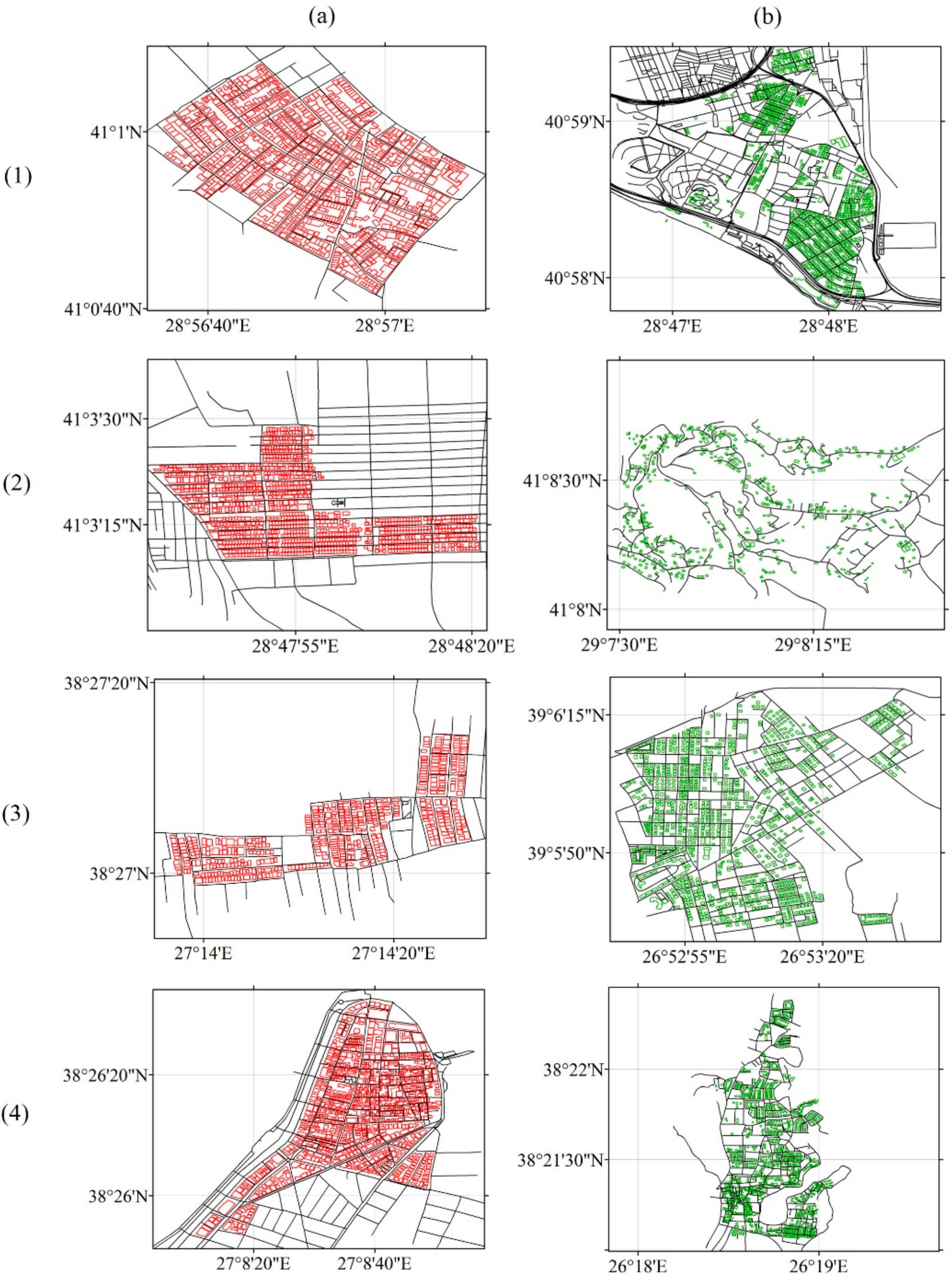
OSM buildings in Istanbul and Izmir, where urban areas are concentrated, were selected to observe the drawing behavior of the volunteers (Figure 1). The geometric properties of the points constituting the buildings were examined in terms of the adjacency types: attached (Figure 2a) and detached (Figure 2b). This study was conducted with eight building groups representing the adjacency types (Table 1). As seen in Figure 2, each group consists of the buildings with one of the adjacency types. The number and place of the groups were selected considering a scattered representation of the heterogeneous data.
A general belief is that in urban locations, detached houses are relatively small buildings compared to attached apartments. However, our study area also consists of detached apartments of greater sizes. Mean area per building represents the average building area in each group (Table 1). It shows that there is no correlation between building size and adjacency type. This case also highlights that an adjacency classification needs several complex measures, rather than simply the polygon area.
2.2. The Proposed Approach
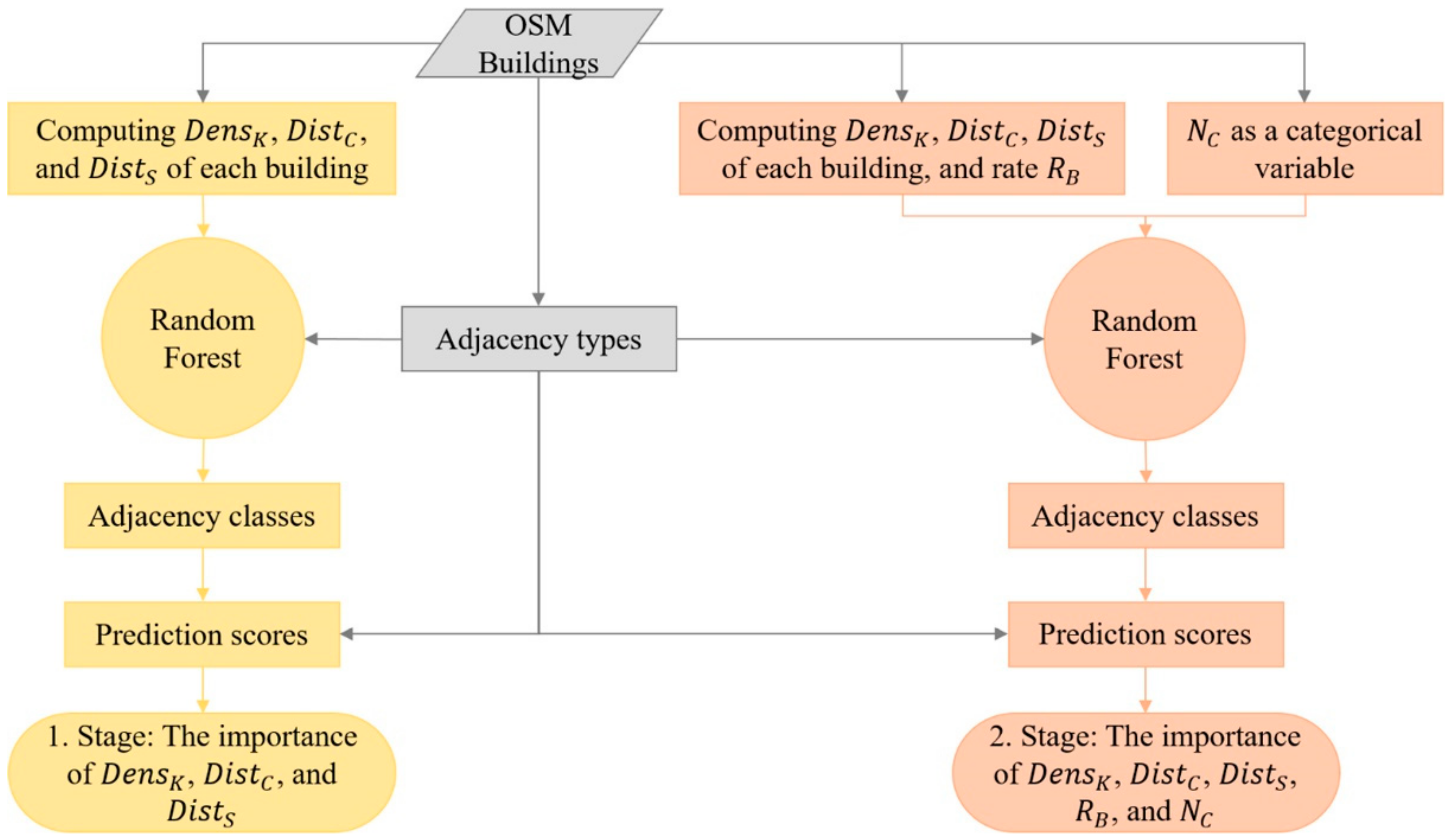
The proposed approach uses some of the geometric properties of the points constituting a building (corner points) to evaluate drawing behavior. To assess different kinds of measures, previous studies have used data mining techniques [6,26,32,33]. Basiri et al. [15] measured the scores of some of ML classifiers and found that K-nearest neighbor and random forest classifiers are suitable for geometric and geographic type classifications, respectively. Furthermore, Pazoky and Pahlavani [34] recently compared several ML classifiers with the centrality measures of OSM data for data enrichment. Random forest became prominent in terms of the prediction scores both in a singular scenario and in a multi-classifier fused with support vector machine. In this study, the proposed approach also uses random forest, with the geometric properties of training data to classify the test data. Figure 3 shows the outline of the proposed workflow for adjacency classification and inferring feature importance. After the first classification conducted using the properties, it assesses the prediction scores by comparing the predicted classes with the actual classes (adjacency types) of the test data.
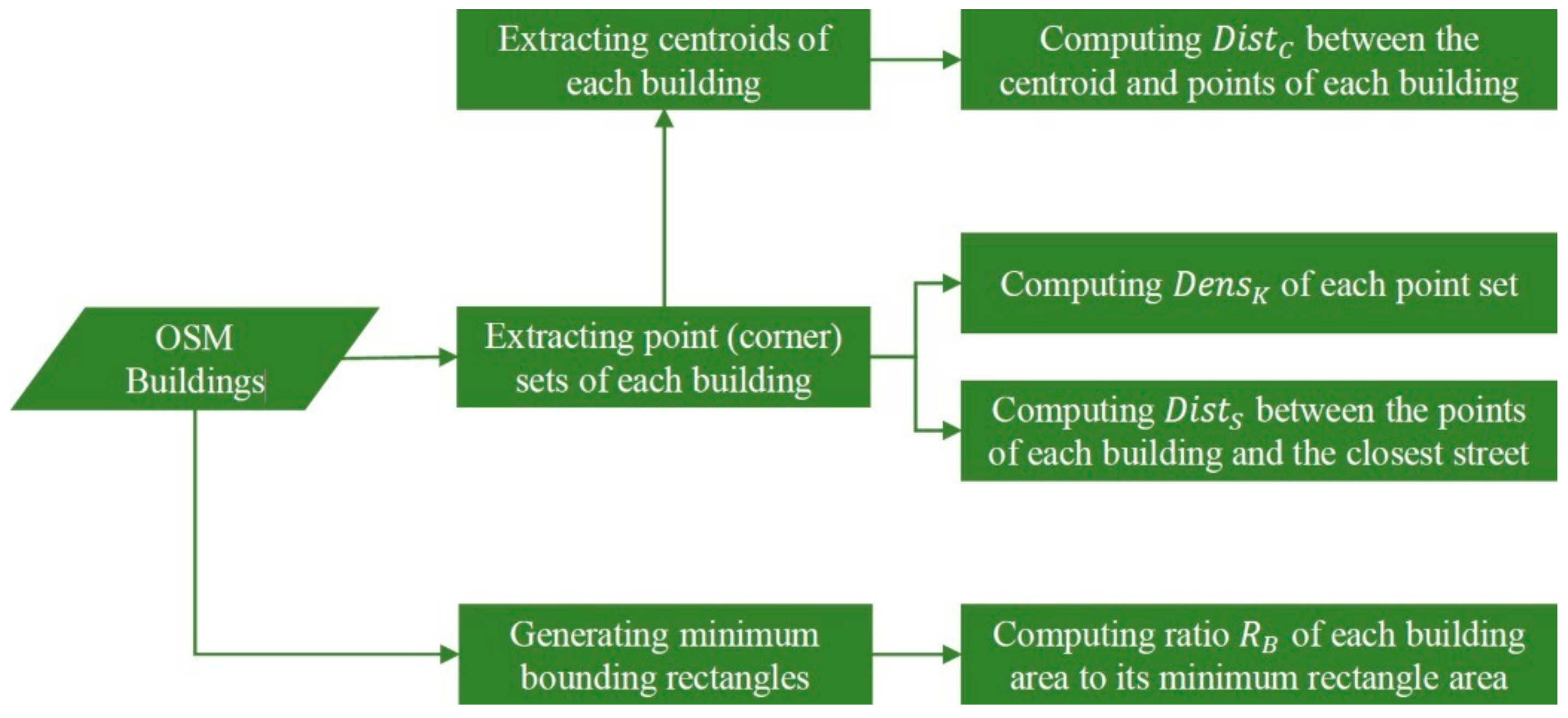
In this study, popular similarity measures such as point-to-point and point-to-line distances [35], density [36,37], and rectangularity [38,39] are used. For each corner point, the measures kernel density value , distance to building centroid , and shortest distance to closest street are computed. Figure 4 summarizes the computation schema of the geometric measures. The measures of the first point drawn in each building and the sum of the respecting measure values of all points are computed. In other words, each building includes the values:
- : kernel density of first point,
- : sum of kernel density values of all points of the building,
- : distance between first point and building centroid,
- : sum of distances of all points to centroid,
- : shortest distance between first point and closest street, and
- : sum of distances of all points to their closest streets.
The proposed approach uses the adjacency types of buildings as dependent variables to measure the effect of , , and values on volunteers’ selection of their first point. Adjacency types are predicted using the values (independent variables). Then, the prediction scores are obtained by comparing the real (actual) adjacency types with the predicted classes. The importance of , , and measures in predicting the adjacency types are determined (1st stage). In other words, the relationships between the spatial properties of the first point and the building’s adjacency class are inferred from the sort of the importance values. Similar relationships are established for building rectangularity value and city name (2nd stage).
All corner points that constitute a building represent the point set of that building. Since the approach relies on the observation of the first point selection in each building, rather than a whole dataset, it uses only the respective point set, rather than the whole point sets, to calculate the kernel density. The density is calculated considering only the target building. In other words, the effects of the buildings on each other are disregarded. This is because of how significant the density value in the polygon is when selecting the first point on the represented building. The kernel density tool in ArcMap 10 [40] was used with respect to Silverman’s [36] quartic formulation. The density is calculated in each polygon. Then, a density value from the nearest pixel is assigned to each corner point.
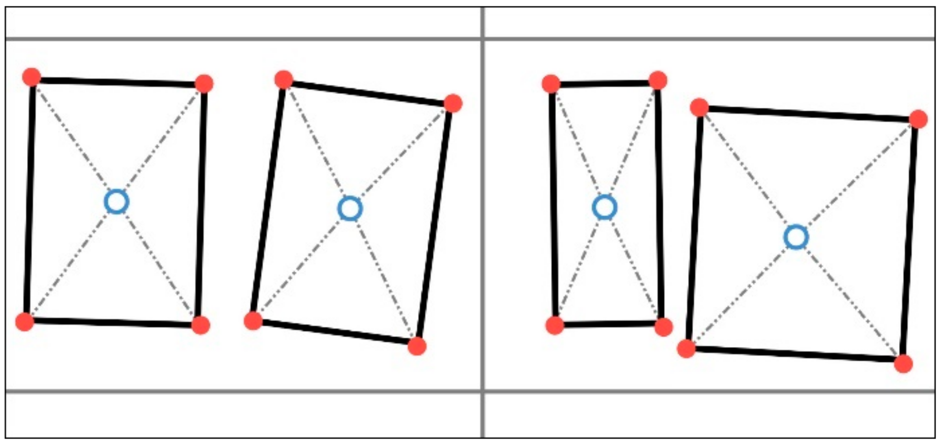
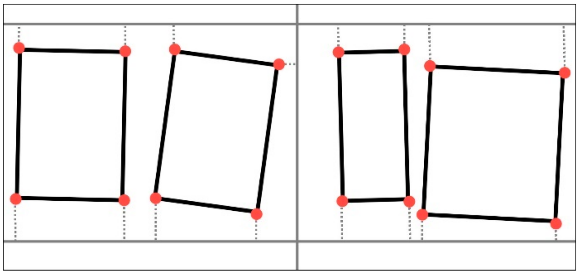
Moreover, the distances between each point in the point set and the building centroid, and the shortest distances between each point in the point set and the closest street are measured in Euclidean geometry as in Figure 5 and Figure 6, respectively. The proposed approach uses the simple rectangularity estimation as the ratio of the polygon’s area against the area of its minimum bounding rectangle [39].
The proposed approach is dependent on the prediction scores of the classification results. In this study, it is intended to predict most of the case data to examine the contributors’ drawing behavior and make reliable inferences. Therefore, more prediction scores over 50% represent more confidence in the approach.
3. Results and Evaluation
This study was conducted with the building groups in Istanbul and Izmir (Table 1 and Figure 2). While 5600 buildings were used randomly as training data, the adjacency types of the remaining 1400 buildings have been predicted. The prediction scores of the test data were obtained by comparing the predicted classes and real adjacency types. While precision can be defined as the positive predictive value or the ability of the classifier, recall is the sensitivity and ability of the classifier to find all the positive samples [41]. F-score represents the balance between precision and recall. It is a weighted harmonic mean of the precision and recall, where the score reaches its best value at 1 and its worst at 0 [41]. Table 2 and Table 3 present the results of the first and second stages, respectively.
In the first stage of the study, the adjacency type of the buildings was predicted using only , , , , , and measures. The F-score of the experiment was determined as 77% (Table 2). In the second stage, and were added to the existing measures for second training. As a result, the score increased to 83% when all variables were used. Table 2 and Table 3 show that most of the classes have been predicted. However, the prediction scores do not demonstrate how the measures affect the results. Therefore, an additional evaluation is necessary to comprehend which measure is most effective in prediction.
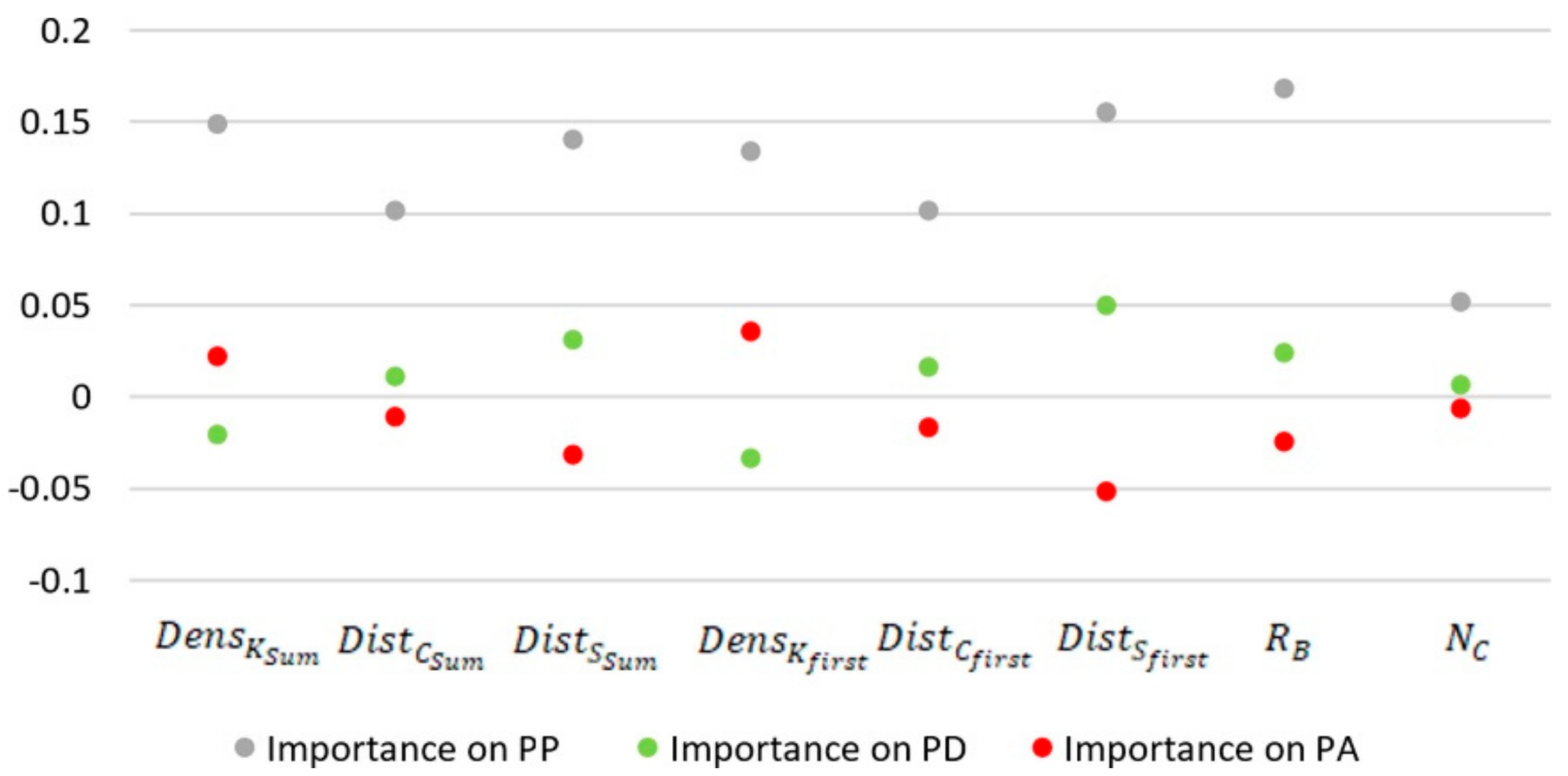
Generally, the importance of a measure is computed as the (normalized) total reduction of the criterion brought about by that measure [41]. The importance comes from the base formula of Gini impurity [42]. After determining the importance of each measure in the prediction process (PP), the measure importance in predicting the relevant class (i.e., adjacency type) was also calculated by (1).
where is the importance of measure i in predicting the specific adjacency type, is the scaled value of measure i, and is the importance of measure i in PP. The formula finds the importance by multiplying the mean value of each measure in each predicted adjacency type by the corresponding measure importance. As a result, the graph below summarizes the importance of each of the measures in predicting attached (PA in Figure 7) and detached (PD in Figure 7) types. The sign of the importance value in the graph helps us to interpret how much more (+) or less (−) important the relevant value is. The higher the kernel density of both the first point () and all points (), the more important the kernel density is in estimating attached buildings because the sign is positive in the graph (Figure 7). Conversely, we can say that the lower the density, the more effective it is in predicting detached buildings because the sign is negative. Similarly, in predicting the detached buildings it is more effective if the first point is far from the street, while it is more effective to have the first point closer to the street in predicting the attached buildings. Additionally, in the attached buildings it is more important that the first point is closer to the centroid, while it is more important that it is farther away in the detached. These results comprise a trend showing that the first points of attached buildings have greater density and are closer to the street and the centroid. The detached buildings have the opposite trend. It is possible to order the importance of the measures. The distance values and kernel density of the first point are more important than the total distances and kernel density of all points. Moreover, a lower rectangularity value is more significant in the attached buildings, whereas the opposite is the case for the detached. Finally, the city names have little effect on PA and PD; therefore, making inferences about the adjacency types according to the name measure requires additional experiments in different cities.
4. Conclusions
Assessing the drawing trends among OSM buildings is challenging because buildings are constituted by a limited number of points compared to other geographical features, such as roads, streams, land use, or sea. This study used an ML classifier to interpret the building geometry contributions in OSM. Four geometric measures (, , , and ) and one semantic measure () were used to assess the drawing behavior of the volunteers. Common trends were determined among the OSM drawings, which were generated by crowdsourced contributions in Istanbul and Izmir. It was observed that there are relationships between the adjacency type of the building and the first drawing action of OSM volunteers. For attached buildings, there is a trend towards drawing the first point where point density is large and close to the street and the centroid. This is the opposite in the detached buildings. It was also possible to determine an order of importance among the measures. Distance to the street is more important than kernel density, and density is more important than distance to the building centroid. In other words, for attached buildings, the volunteers focused on drawing the first point of the building in the parts closest to the street, and, among the alternatives, they decided to draw it in the place at which point density is higher and the distance to centroid is smaller. The results also enabled the inference that, for detached buildings, OSM volunteers paid more attention to open spaces when drawing the first points because the first-drawn points have lower density and are further both from streets and building centroids than for the attached ones.
This study shows that an ML classifier and feature importance based on prediction results can be used to determine the drawing trends of OSM contributors. The novelty of the study is that it reveals common drawing trends in building-mapping actions.
It appeared that adding the city name at the second stage had little effect (rather than no effect) in predicting the adjacency classes, even though equal numbers of buildings were used in both cities. This means that volunteers may have specific drawing habits in a particular region. However, to substantiate the assumption, buildings in more than two cities should be studied in the future.
The experimental test presents the drawing characteristics of the volunteers who contributed to OSM in the study areas. Both Istanbul and Izmir are metropolitan cities. Therefore, different types of urban or rural areas may give different results.
The main limitation of the study is the measures used as the independent variables in PP. Apart from the measures, the tags contributed by OSM volunteers can also be evaluated as independent variables and a similar study may be conducted. Thus, possible crowdsourced trends can be interpreted with geometric properties and tags.
Funding
This research received no external funding.
Data Availability Statement
The case data downloaded from OpenStreetMap (http://download.geofabrik.de/ (accessed on 20 October 2021)) are also openly available in geo-database format at [figshare repository] DOI: 10.6084/m9.figshare.14573556.
Conflicts of Interest
The author declares no conflict of interest.
References
- Goodchild, M.F. Citizens as sensors: The world of volunteered geography. GeoJournal 2007, 69, 211–221. [Google Scholar] [CrossRef] [Green Version]
- Heipke, C. Crowdsourcing geospatial data. ISPRS J. Photogramm. 2010, 65, 550–557. [Google Scholar] [CrossRef]
- Kang, X. Graph-based synchronous collaborative mapping. Geocarto. Int. 2015, 30, 28–47. [Google Scholar] [CrossRef]
- Mooney, P.; Corcoran, P.; Winstanley, A.C. Towards quality metrics for OpenStreetMap. In Proceedings of the 18th SIGSPATIAL International Conference on Advances in Geographic Information Systems, San Jose, CA, USA, 2–5 November 2010; pp. 514–517. [Google Scholar] [CrossRef] [Green Version]
- Mooney, P.; Corcoran, P. The annotation process in OpenStreetMap. Trans. GIS 2012, 16, 561–579. [Google Scholar] [CrossRef]
- Jilani, M.; Corcoran, P.; Bertolotto, M. Automated highway tag assessment of OpenStreetMap road networks. In Proceedings of the 22nd ACM SIGSPATIAL International Conference on Advances in Geographic Information Systems, Dallas/Fort Worth, TX, USA, 4–7 November 2014; pp. 449–452. [Google Scholar] [CrossRef] [Green Version]
- Davidovic, N.; Mooney, P.; Stoimenov, L. An analysis of tagging practices and patterns in urban areas in OpenStreetMap. In Proceedings of the AGILE 2016 Conference, Helsinki, Finland, 14–17 June 2016. [Google Scholar]
- Hacar, M. Analyzing the Contribution Trends of Volunteers by Comparing Tag Metadata of OpenStreetMap Residential Roads [Original title in Turkish: OpenStreetMap Yerleşim-içi Yollarına Ait Etiket Bilgilerinin Karşılaştırılmasıyla Gönüllülerin Katkı Sağlama Eğilimlerinin İncelenmesi]. Harita. Dergisi. 2020, 164, 77–87. [Google Scholar]
- Mobasheri, A.; Deister, J.; Dieterich, H. Wheelmap: The wheelchair accessibility crowdsourcing platform. Open Geospat. Data Softw. Stand. 2017, 2, 1–7. [Google Scholar] [CrossRef]
- Guan, W.W.; Bol, P.K.; Lewis, B.G.; Bertrand, M.; Berman, M.L.; Blossom, J.C. WorldMap—A geospatial framework for collaborative research. Ann. GIS 2012, 18, 121–134. [Google Scholar] [CrossRef]
- Ballatore, A.; Jokar Arsanjani, J. Placing Wikimapia: An exploratory analysis. Int. J. Geogr. Inf. Sci. 2019, 33, 1633–1650. [Google Scholar] [CrossRef]
- OpenStreetMap Wiki. Welcome to OpenStreetMap. Available online: https://wiki.openstreetmap.org/wiki/Main_Page (accessed on 20 October 2021).
- Neis, P.; Zipf, A. Analyzing the contributor activity of a volunteered geographic information project—The case of OpenStreetMap. ISPRS Int. J. Geo.-Inf. 2012, 1, 146–165. [Google Scholar] [CrossRef]
- OpenStreetMap Wiki. Planet.osm. Available online: https://wiki.openstreetmap.org/wiki/Planet.osm (accessed on 20 October 2021).
- Basiri, A.; Amirian, P.; Mooney, P. Using crowdsourced trajectories for automated OSM data entry approach. Sensors 2016, 16, 1510. [Google Scholar] [CrossRef] [Green Version]
- Haklay, M. How good is volunteered geographical information? A comparative study of OpenStreetMap and Ordnance Survey datasets. Environ. Plan. B 2010, 37, 682–703. [Google Scholar] [CrossRef] [Green Version]
- Girres, J.F.; Touya, G. Quality assessment of the French OpenStreetMap dataset. Trans. GIS 2010, 14, 435–459. [Google Scholar] [CrossRef]
- Mondzech, J.; Sester, M. Quality analysis of OpenStreetMap data based on application needs. Cartographica 2011, 46, 115–125. [Google Scholar] [CrossRef]
- Da Costa, J.N. Novel tool for examination of data completeness based on a comparative study of VGI data and official building datasets. Geodetski Vestnik 2016, 60, 495–508. [Google Scholar] [CrossRef]
- Zhang, H.; Malczewski, J. Accuracy Evaluation of the Canadian OpenStreetMap Road Networks. IJGER 2018, 5, 1–14. Available online: https://dc.uwm.edu/ijger/vol5/iss2/1/ (accessed on 20 October 2021).
- Mobasheri, A.; Zipf, A.; Francis, L. OpenStreetMap data quality enrichment through awareness raising and collective action tools—experiences from a European project. Geo-Spat. Inf. Sci. 2018, 21, 234–246. [Google Scholar] [CrossRef] [Green Version]
- Mohammadi, N.; Sedaghat, A. A framework for classification of volunteered geographic data based on user’s need. Geocarto Int. 2021, 36, 1276–1291. [Google Scholar] [CrossRef]
- Corcoran, P.; Mooney, P.; Bertolotto, M. Analysing the growth of OpenStreetMap networks. Spat. Stat. 2013, 3, 21–32. [Google Scholar] [CrossRef] [Green Version]
- Zhao, P.; Jia, T.; Qin, K.; Shan, J.; Jiao, C. Statistical analysis on the evolution of OpenStreetMap road networks in Beijing. Physica A 2015, 420, 59–72. [Google Scholar] [CrossRef]
- Hacar, M.; Kılıç, B.; Şahbaz, K. Analyzing OpenStreetMap road data and characterizing the behavior of contributors in Ankara, Turkey. ISPRS Int. J. Geo.-Inf. 2018, 7, 400. [Google Scholar] [CrossRef] [Green Version]
- Basiri, A.; Jackson, M.; Amirian, P.; Pourabdollah, A.; Sester, M.; Winstanley, A.; Moore, T.; Zhang, L. Quality assessment of OpenStreetMap data using trajectory mining. Geo-Spat. Inf. Sci. 2016, 19, 56–68. [Google Scholar] [CrossRef] [Green Version]
- Hacar, M. Using geometric and semantic attributes for semi-automated tag identification in OpenStreetMap data. In Proceedings of the GISRUK 2021, Cardiff, UK, 14–16 April 2021. [Google Scholar] [CrossRef]
- Wright, J.K. Map makers are human: Comments on the subjective in maps. Geogr. Rev. 1942, 32, 527–544. [Google Scholar] [CrossRef]
- Mooney, P.; Corcoran, P. Characteristics of heavily edited objects in OpenStreetMap. Future Internet 2012, 4, 285–305. [Google Scholar] [CrossRef] [Green Version]
- OpenStreetMap Wiki. Map Features. Available online: https://wiki.openstreetmap.org/wiki/Map_Features (accessed on 20 October 2021).
- Global Administrative Areas. GADM Database. Available online: http://www.gadm.org/ (accessed on 20 October 2021).
- Mobasheri, A.; Huang, H.; Degrossi, L.C.; Zipf, A. Enrichment of OpenStreetMap data completeness with sidewalk geometries using data mining techniques. Sensors 2018, 18, 509. [Google Scholar] [CrossRef] [PubMed] [Green Version]
- Mocnik, F.B.; Mobasheri, A.; Zipf, A. Open source data mining infrastructure for exploring and analysing OpenStreetMap. Open Geospat. Data Softw. Stand. 2018, 3, 1–15. [Google Scholar] [CrossRef]
- Pazoky, S.H.; Pahlavani, P. Developing a multi-classifier system to classify OSM tags based on centrality parameters. Appl. Earth Obs. Geoinf. 2021, 104, 102595. [Google Scholar] [CrossRef]
- Mustière, S.; Devogele, T. Matching networks with different levels of detail. GeoInformatica 2008, 12, 435–453. [Google Scholar] [CrossRef]
- Silverman, B.W. Density Estimation for Statistics and Data Analysis; Chapman and Hall, CRC Press: London, UK, 1986. [Google Scholar]
- Gibin, M.; Longley, P.; Atkinson, P. Kernel density estimation and percent volume contours in general practice catchment area analysis in urban areas. In Proceedings of the GISRUK 2007, Kildare, Ireland, 11–13 April 2007; pp. 282–288. [Google Scholar]
- Fan, H.; Zipf, A.; Fu, Q.; Neis, P. Quality assessment for building footprints data on OpenStreetMap. Int. J. Geogr. Inf. Sci. 2014, 28, 700–719. [Google Scholar] [CrossRef]
- Rosin, P.L. Measuring rectangularity. Mach. Vision Appl. 1999, 11, 191–196. [Google Scholar] [CrossRef]
- ArcMap. How Kernel Density Works-ArcMap. Documentation. (n.d.). Available online: https://desktop.arcgis.com/en/arcmap/latest/tools/spatial-analyst-toolbox/how-kernel-density-works.htm (accessed on 20 October 2021).
- Pedregosa, F.; Varoquaux, G.; Gramfort, A.; Michel, V.; Thirion, B.; Grisel, O.; Blondel, M.; Prettenhofer, P.; Weiss, R.; Dubourg, V.; et al. Scikit-learn: Machine learning in Python. J. Mach. Learn Res. 2011, 12, 2825–2830. [Google Scholar]
- Breiman, L.; Friedman, J.; Stone, C.J.; Olshen, R.A. Classification and Regression Trees; Chapman and Hall, CRC Press: London, UK, 1984. [Google Scholar]
Figure 1.
Location of attached (red points) and detached (green points) building groups in Istanbul and Izmir (map data taken from the Global Administrative Areas [31] database).
Figure 1.
Location of attached (red points) and detached (green points) building groups in Istanbul and Izmir (map data taken from the Global Administrative Areas [31] database).

Figure 2.
Attached (a) and detached (b) buildings.

Figure 3.
The workflow of the proposed approach.

Figure 4.
The computation schema of the measures.

Figure 5.
Buildings (black continuous), point sets (red), centroids (blue), (grey dashed), and streets (grey continuous).
Figure 5.
Buildings (black continuous), point sets (red), centroids (blue), (grey dashed), and streets (grey continuous).

Figure 6.
Buildings (black continuous), point sets (red), (grey dashed), and streets (grey continuous).
Figure 6.
Buildings (black continuous), point sets (red), (grey dashed), and streets (grey continuous).

Figure 7.
The importance of measures on predicting the adjacency types: PP as prediction process, PD as predicting the detached buildings, and PA as predicting the attached buildings.
Figure 7.
The importance of measures on predicting the adjacency types: PP as prediction process, PD as predicting the detached buildings, and PA as predicting the attached buildings.


Table 1.
The statistics of building groups.
| Building Group | City | Adjacency Type | Number of Buildings | Mean Area per Building (m2) |
|---|---|---|---|---|
| Group 1 (1a in Figure 2) | Istanbul | Attached | 1000 | 184.4 |
| Group 2 (2a in Figure 2) | Istanbul | Attached | 1000 | 163.1 |
| Group 3 (3a in Figure 2) | Izmir | Attached | 500 | 127.4 |
| Group 4 (4a in Figure 2) | Izmir | Attached | 1000 | 217.8 |
| Group 5 (1b in Figure 2) | Istanbul | Detached | 1000 | 475.8 |
| Group 6 (2b in Figure 2) | Istanbul | Detached | 500 | 142.9 |
| Group 7 (3b in Figure 2) | Izmir | Detached | 1000 | 155.1 |
| Group 8 (4b in Figure 2) | Izmir | Detached | 1000 | 176.4 |
Table 2.
Test results of the prediction scores at stage 1.
| Adjacency Type | Precision (%) | Recall (%) | F-Score (%) | Number of Buildings |
|---|---|---|---|---|
| Detached | 77 | 79 | 78 | 713 |
| Attached | 77 | 75 | 76 | 687 |
| Avg/total | 77 | 77 | 77 | 1400 |
Table 3.
Test results of the prediction scores at stage 2.
| Adjacency Type | Precision (%) | Recall (%) | F-Score (%) | Number of Buildings |
|---|---|---|---|---|
| Detached | 83 | 84 | 83 | 713 |
| Attached | 83 | 82 | 83 | 687 |
| Avg/total | 83 | 83 | 83 | 1400 |
Publisher’s Note: MDPI stays neutral with regard to jurisdictional claims in published maps and institutional affiliations. |
© 2022 by the author. Licensee MDPI, Basel, Switzerland. This article is an open access article distributed under the terms and conditions of the Creative Commons Attribution (CC BY) license (https://creativecommons.org/licenses/by/4.0/).
Share and Cite
MDPI and ACS Style
Hacar, M. Analyzing the Behaviors of OpenStreetMap Volunteers in Mapping Building Polygons Using a Machine Learning Approach. ISPRS Int. J. Geo-Inf. 2022, 11, 70. https://doi.org/10.3390/ijgi11010070
AMA Style
Hacar M. Analyzing the Behaviors of OpenStreetMap Volunteers in Mapping Building Polygons Using a Machine Learning Approach. ISPRS International Journal of Geo-Information. 2022; 11(1):70. https://doi.org/10.3390/ijgi11010070
Chicago/Turabian StyleHacar, Müslüm. 2022. "Analyzing the Behaviors of OpenStreetMap Volunteers in Mapping Building Polygons Using a Machine Learning Approach" ISPRS International Journal of Geo-Information 11, no. 1: 70. https://doi.org/10.3390/ijgi11010070
Note that from the first issue of 2016, this journal uses article numbers instead of page numbers. See further details here.