Dynamic Estimation of Individual Exposure Levels to Air Pollution Using Trajectories Reconstructed from Mobile Phone Data


Abstract
:1. Introduction
- (1)
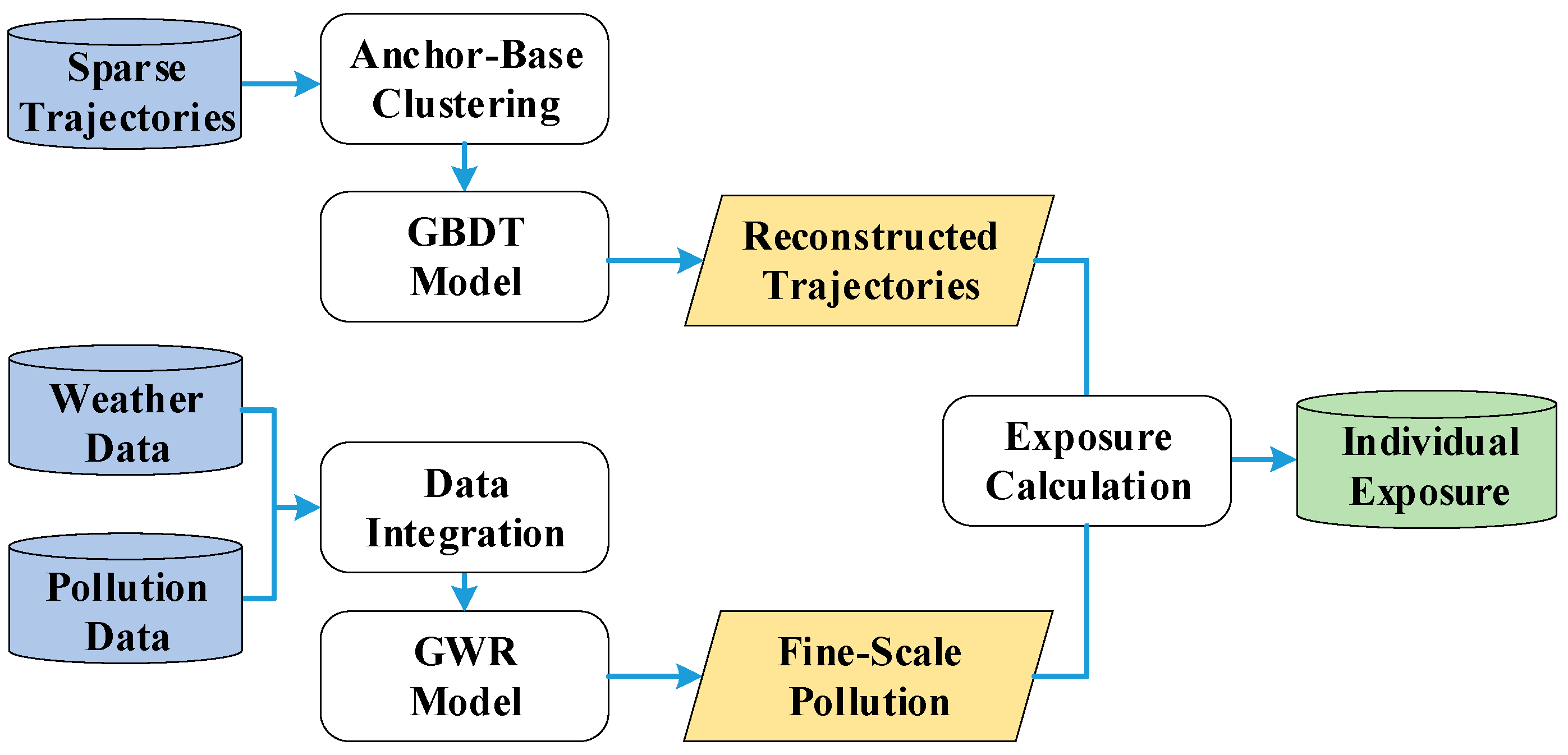
- We present a novel individual air pollution exposure estimate method. Our method mitigates the gap of spatiotemporal resolution between air pollution monitoring data and mobile phone data, which helps improve the accuracy and reliability of fine-scale air pollution exposure estimation.
- (2)
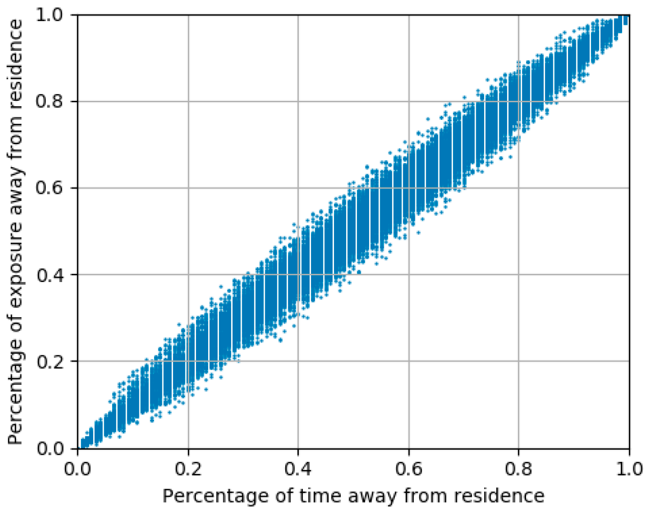
- By comparing the three different types of exposure estimates using reconstructed mobile phone trajectories, recorded mobile phone trajectories, and residential locations, we demonstrate the necessity of trajectory reconstruction in exposure estimation.
- (3)
- Using the city of Shanghai as a case study, we quantitatively analyzed the temporal variations in individual exposures and the spatial distribution of residential areas with high exposure levels using large-scale mobile phone data. It provides a more accurate and comprehensively scientific basis for policy-driven environmental actions and potential health risk reduction.
2. Literature Review
2.1. Air Pollution Exposure Estimates
2.2. Trajectory Reconstruction from Mobile Phone Data
3. Methodology
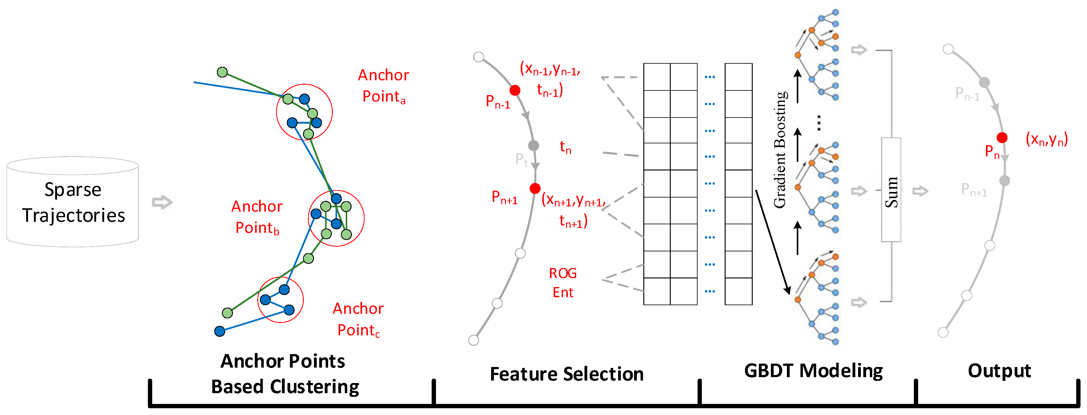
3.1. Anchor-Point Based Trajectory Reconstruction Algorithm
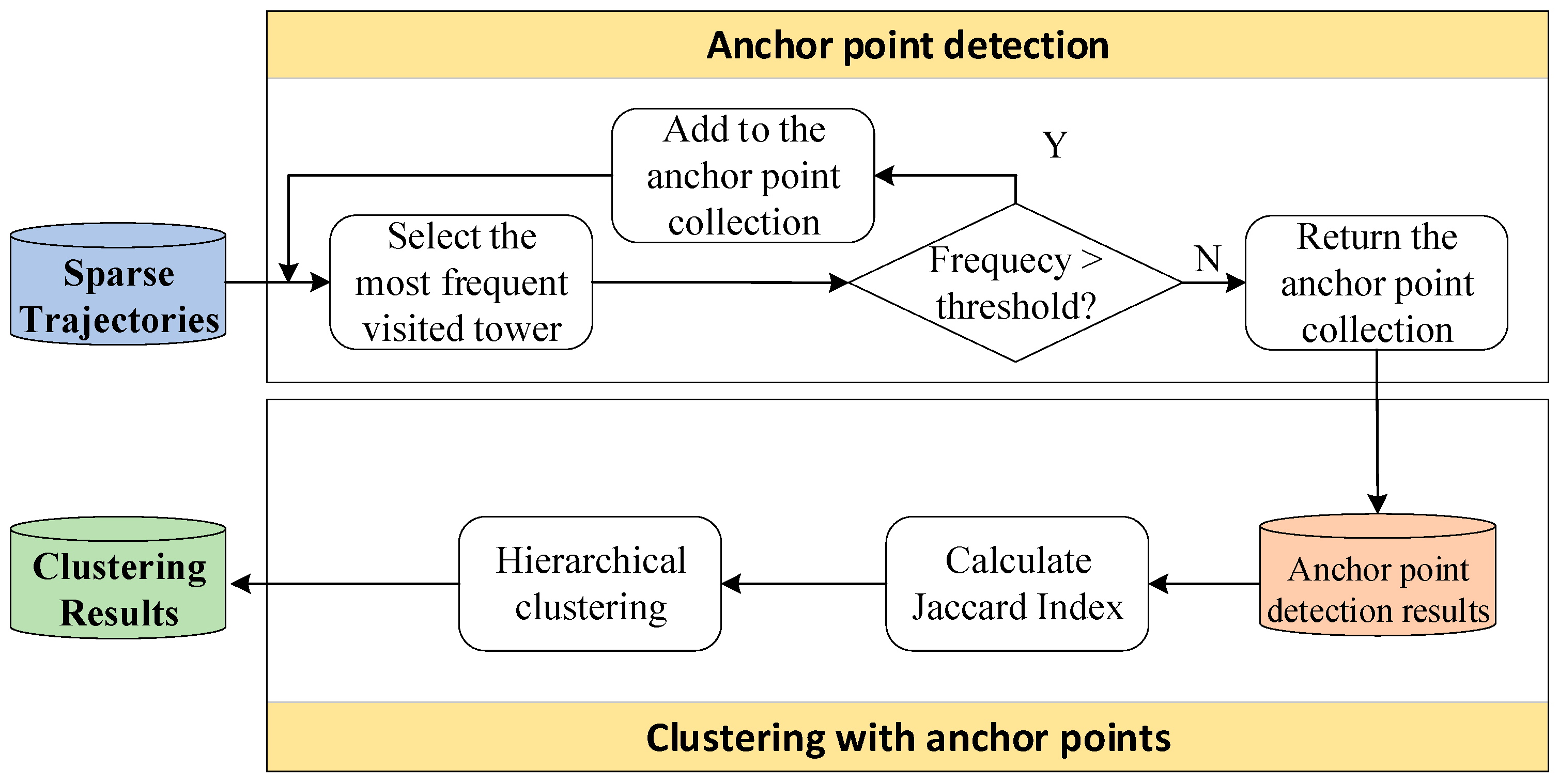
3.1.1. Anchor-Point-Based Clustering
3.1.2. Reconstruction of Clustered Trajectories Using a Gradient Boosting Decision Tree Model
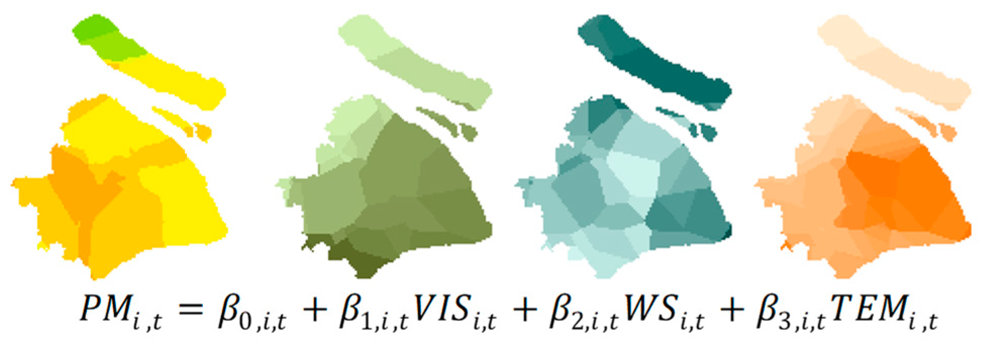
3.2. Estimation of Spatiotemporal Concentrations of Air Pollution
3.3. Dynamic Individual Exposure Calculation
4. Case Study
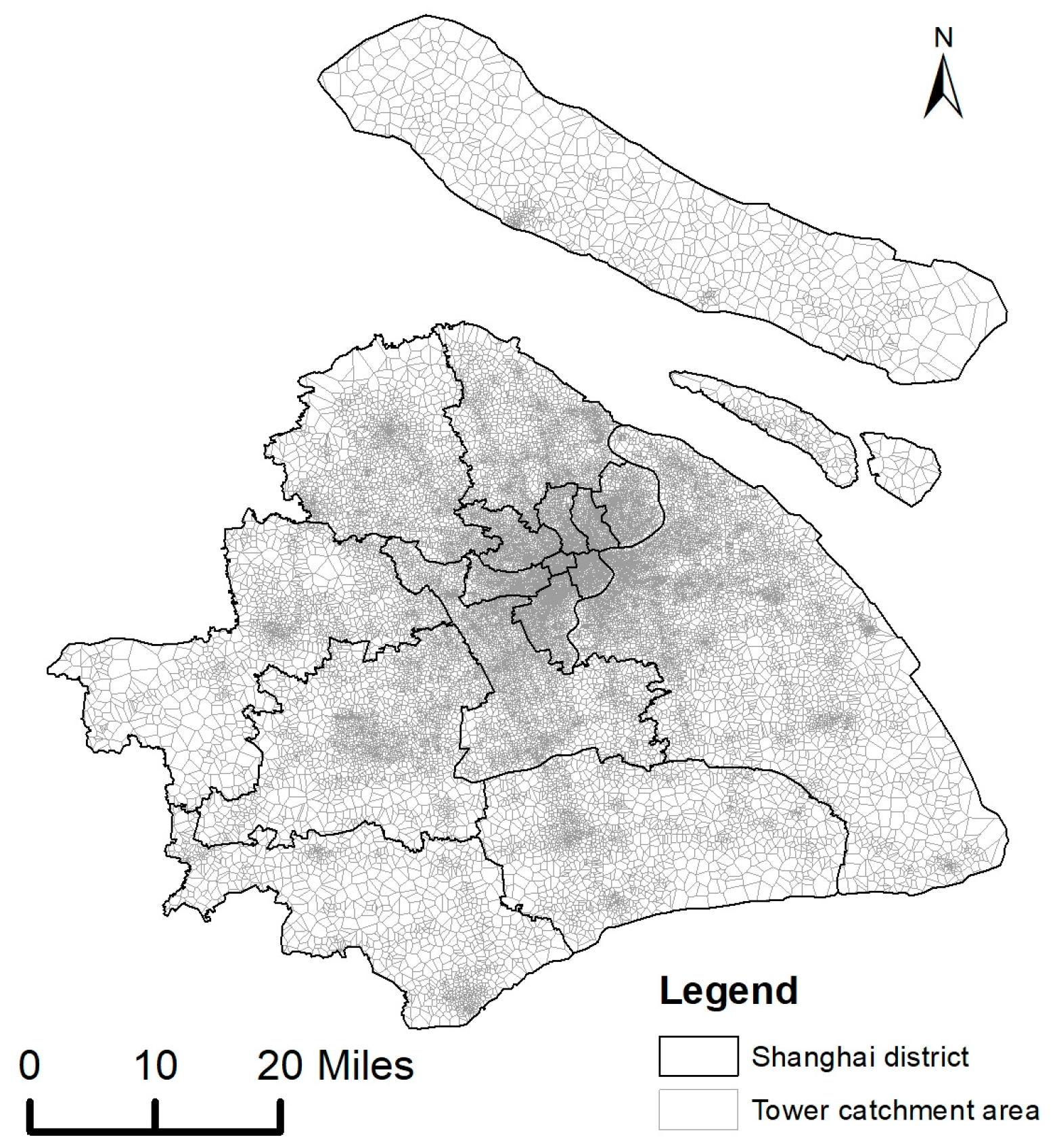
4.1. Data
4.1.1. Mobile Phone Data
4.1.2. Environmental Data
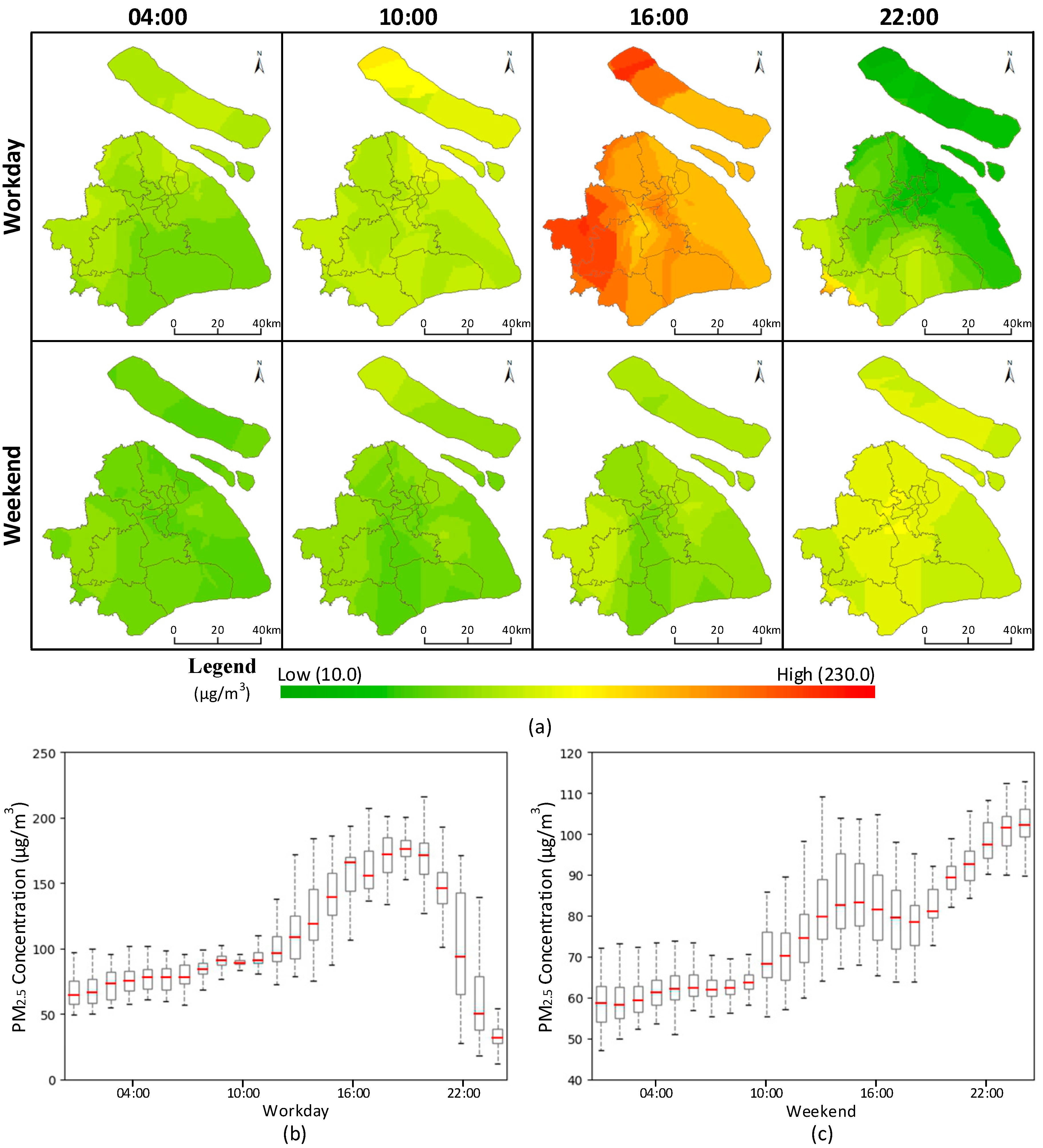
4.2. Spatiotemporal Variability in PM2.5 Concentration
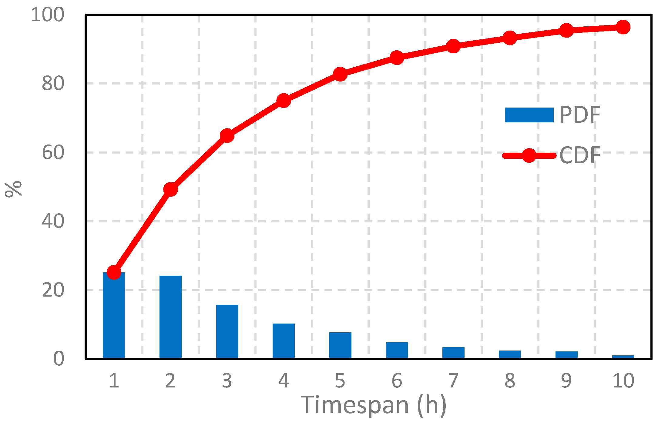
4.3. Performance Evaluation of the Trajectory Reconstruction Algorithm
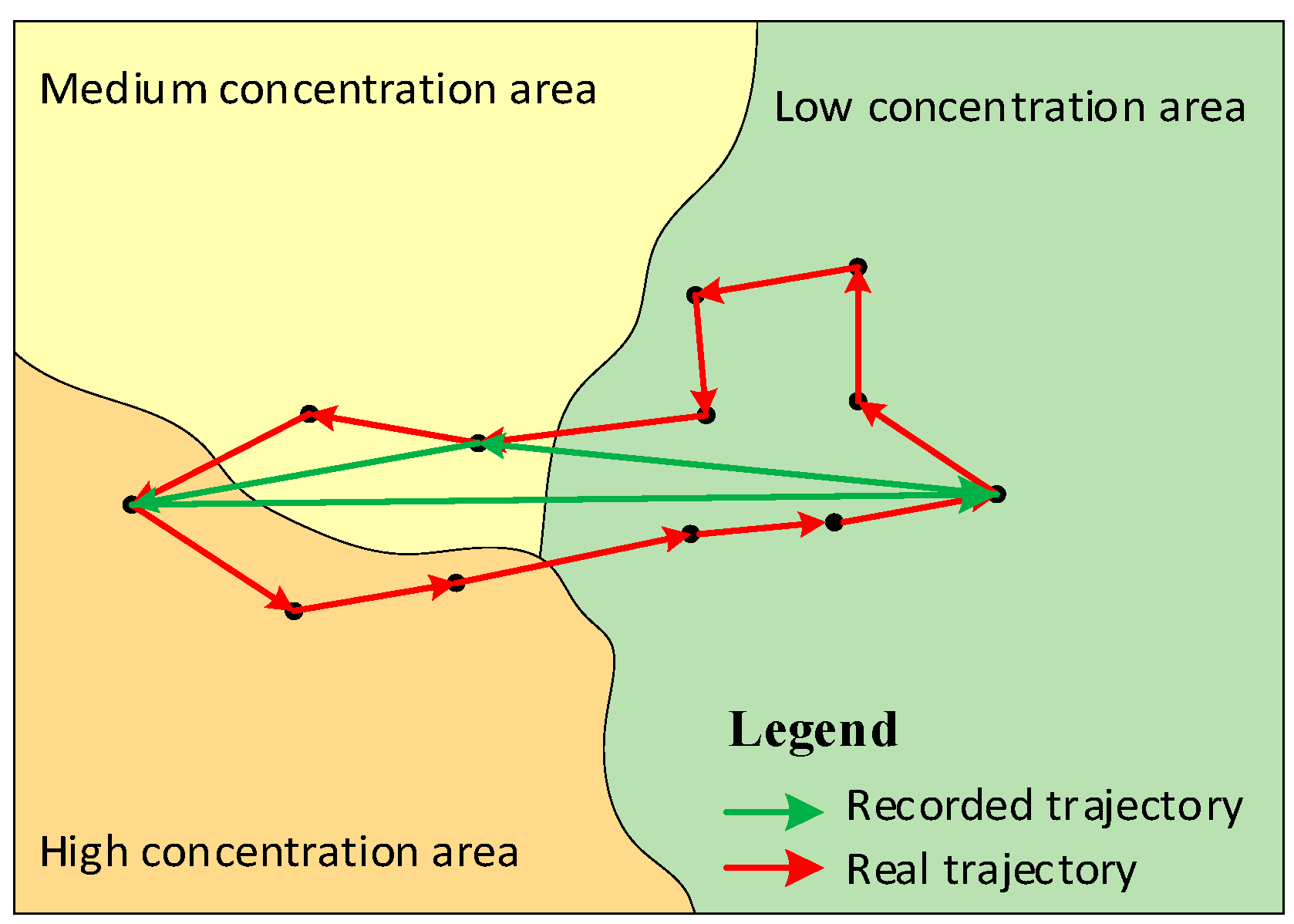
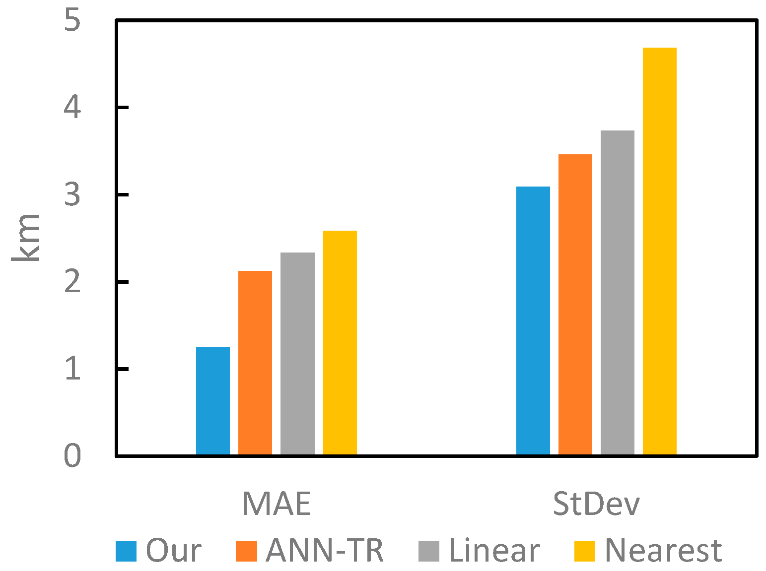
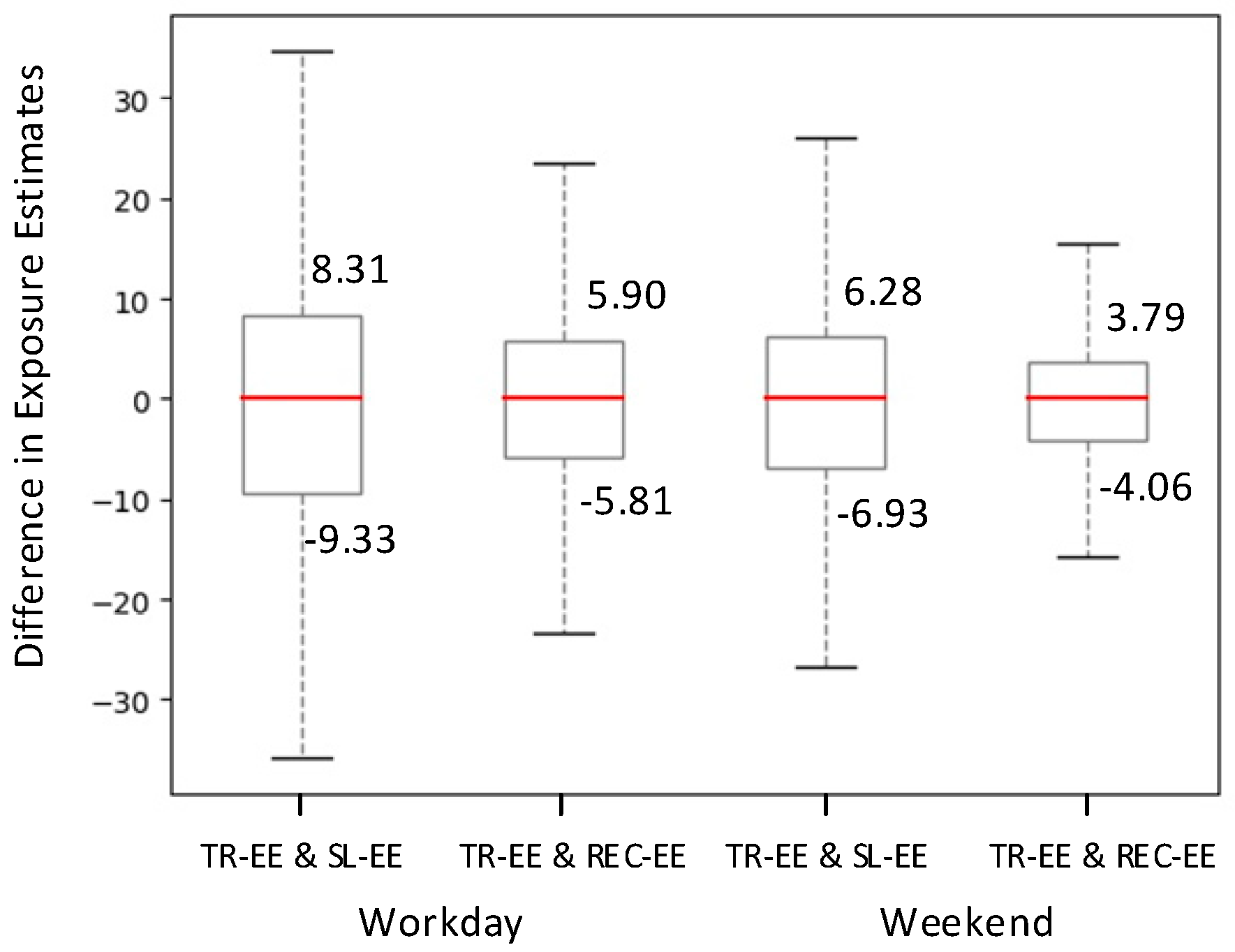
4.4. Comparison with Existing Exposure Estimate Methods
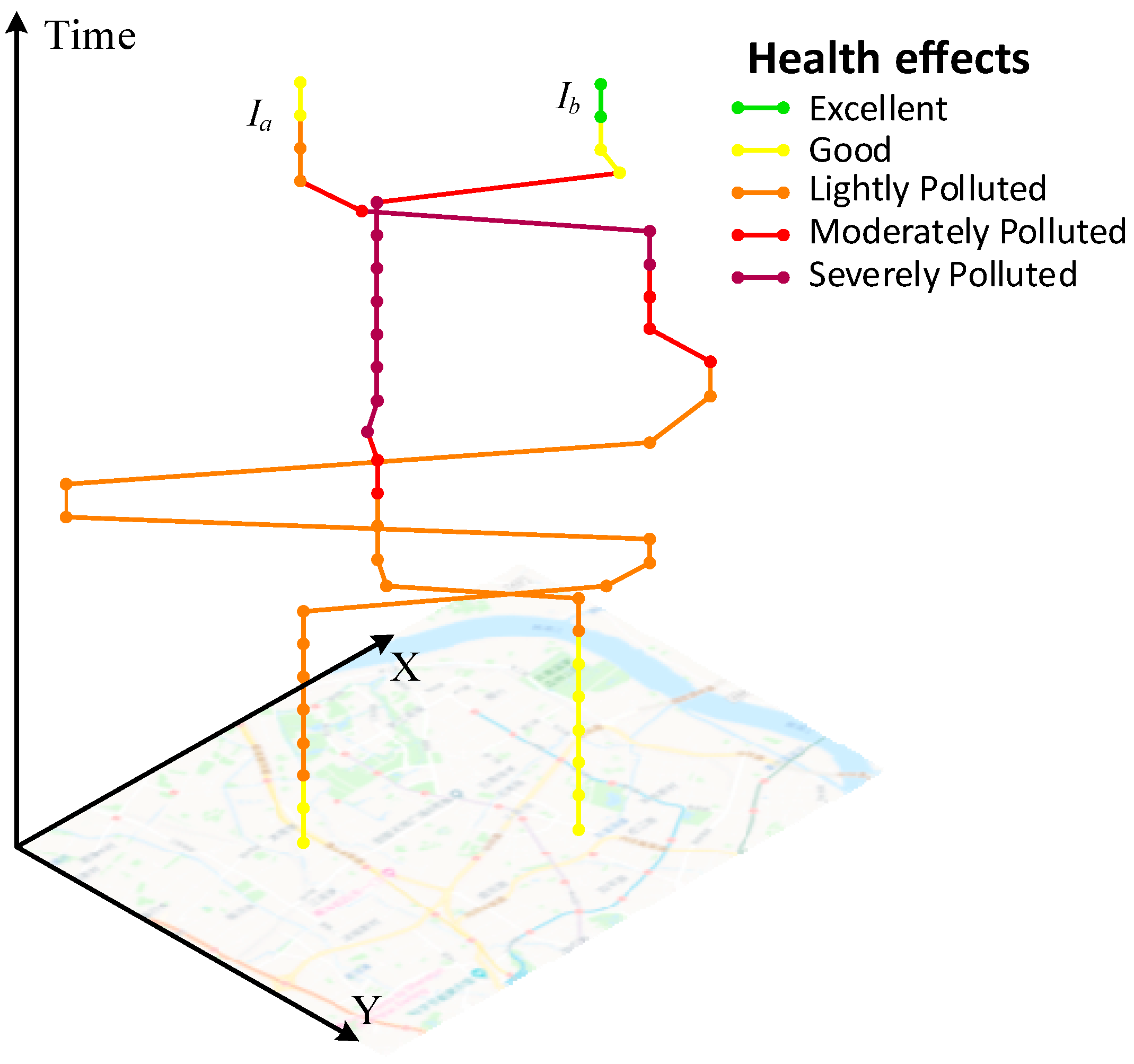
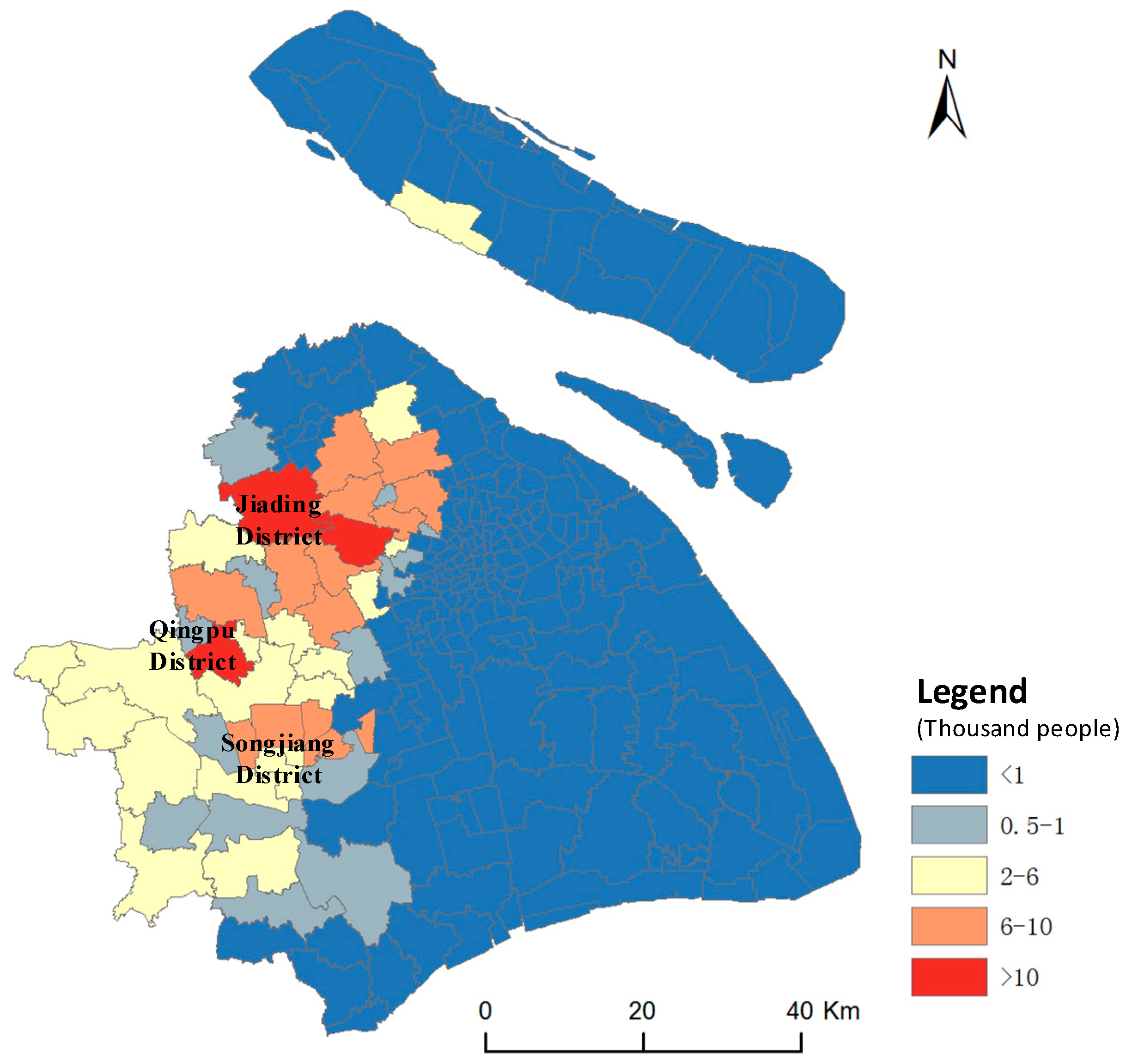
4.5. Potential Health Effects
5. Conclusions
Author Contributions
Funding
Conflicts of Interest
References
- Brunekreef, B.; Holgate, S.T. Air pollution and health. Lancet 2002, 360, 1233–1242. [Google Scholar] [CrossRef]
- Mannucci, P.M.; Franchini, M. Health Effects of Ambient Air Pollution in Developing Countries. Int. J. Environ. Res. Public Health 2017, 14, 1048. [Google Scholar] [CrossRef] [PubMed]
- Dominici, F.; Peng, R.D.; Bell, M.L.; Pham, L.; McDermott, A.; Zeger, S.L.; Samet, J.M. Fine particulate air pollution and hospital admission for cardiovascular and respiratory diseases. JAMA 2006, 295, 1127–1134. [Google Scholar] [CrossRef] [PubMed]
- Goldberg, M. A Systematic Review of the Relation between Long-term Exposure to Ambient Air Pollution and Chronic Diseases. Rev. Environ. Health 2011, 23, 243–298. [Google Scholar] [CrossRef] [PubMed]
- Cohen, A.J.; Brauer, M.; Burnett, R.; Anderson, H.R.; Frostad, J.; Estep, K.; Balakrishnan, K.; Brunekreef, B.; Dandona, L.; Dandona, R.; et al. Estimates and 25-year trends of the global burden of disease attributable to ambient air pollution: An analysis of data from the Global Burden of Diseases Study 2015. Lancet 2017, 389, 1907–1918. [Google Scholar] [CrossRef]
- Lelieveld, J.; Klingmüller, K.; Pozzer, A.; Pöschl, U.; Fnais, M.; Daiber, A.; Münzel, T. Cardiovascular disease burden from ambient air pollution in Europe reassessed using novel hazard ratio functions. Eur. Heart J. 2019, 40, 1590–1596. [Google Scholar] [CrossRef]
- Kwan, M.-P.; Liu, D.; Vogliano, J. Assessing Dynamic Exposure to Air Pollution. In Space-Time Integration in Geography and GIScience: Research Frontiers in the US and China; Kwan, M.-P., Richardson, D., Wang, D., Zhou, C., Eds.; Springer: Dordrecht, The Netherlands, 2015; pp. 283–300. ISBN 978-94-017-9205-9. [Google Scholar]
- Park, Y.M.; Kwan, M.-P. Individual exposure estimates may be erroneous when spatiotemporal variability of air pollution and human mobility are ignored. Health Place 2017, 43, 85–94. [Google Scholar] [CrossRef]
- Chen, B.; Song, Y.; Jiang, T.; Chen, Z.; Huang, B.; Xu, B. Real-Time Estimation of Population Exposure to PM2.5 Using Mobile- and Station-Based Big Data. Int. J. Environ. Res. Public Health 2018, 15, 573. [Google Scholar] [CrossRef]
- Yoo, E.; Rudra, C.; Glasgow, M.; Mu, L. Geospatial Estimation of Individual Exposure to Air Pollutants: Moving from Static Monitoring to Activity-Based Dynamic Exposure Assessment. Ann. Assoc. Am. Geogr. 2015, 105, 1–12. [Google Scholar] [CrossRef]
- Xie, X.; Semanjski, I.; Gautama, S.; Tsiligianni, E.; Deligiannis, N.; Rajan, R.T.; Pasveer, F.; Philips, W. A Review of Urban Air Pollution Monitoring and Exposure Assessment Methods. ISPRS Int. J. Geo-Inf. 2017, 6, 389. [Google Scholar] [CrossRef]
- Mennis, J.; Yoo, E.-H.E. Geographic information science and the analysis of place and health. Trans. GIS 2018, 22, 842–854. [Google Scholar] [CrossRef] [PubMed]
- Kwan, M.-P. From place-based to people-based exposure measures. Soc. Sci. Med. 2009, 69, 1311–1313. [Google Scholar] [CrossRef] [PubMed]
- Lioy, P.J. Exposure Science: A View of the Past and Milestones for the Future. Environ. Health Perspect. 2010, 118, 1081–1090. [Google Scholar] [CrossRef] [PubMed]
- Glasgow, M.L.; Rudra, C.B.; Yoo, E.-H.; Demirbas, M.; Merriman, J.; Nayak, P.; Crabtree-Ide, C.; Szpiro, A.A.; Rudra, A.; Wactawski-Wende, J.; et al. Using smartphones to collect time-activity data for long-term personal-level air pollution exposure assessment. J. Expo. Sci. Environ. Epidemiol. 2016, 26, 356–364. [Google Scholar] [CrossRef]
- Mihăiţă, A.S.; Dupont, L.; Chery, O.; Camargo, M.; Cai, C. Evaluating air quality by combining stationary, smart mobile pollution monitoring and data-driven modelling. J. Clean. Prod. 2019, 221, 398–418. [Google Scholar] [CrossRef]
- Ford, B.; Burke, M.; Lassman, W.; Pfister, G.; Pierce, J.R. Status update: Is smoke on your mind? Using social media to assess smoke exposure. Atmos. Chem. Phys. Discuss. 2017, 17, 7541–7554. [Google Scholar] [CrossRef]
- Song, Y.; Huang, B.; Cai, J.; Chen, B. Dynamic assessments of population exposure to urban greenspace using multi-source big data. Sci. Total Environ. 2018, 634, 1315–1325. [Google Scholar] [CrossRef]
- Song, Y.; Huang, B.; He, Q.; Chen, B.; Wei, J.; Mahmood, R. Dynamic assessment of PM2.5 exposure and health risk using remote sensing and geo-spatial big data. Environ. Pollut. 2019, 253, 288–296. [Google Scholar] [CrossRef]
- Yu, X.; Stuart, A.L.; Liu, Y.; Ivey, C.E.; Russell, A.G.; Kan, H.; Henneman, L.R.; Sarnat, S.E.; Hasan, S.; Sadmani, A.; et al. On the accuracy and potential of Google Maps location history data to characterize individual mobility for air pollution health studies. Environ. Pollut. 2019, 252, 924–930. [Google Scholar] [CrossRef]
- Dewulf, B.; Neutens, T.; Lefebvre, W.; Seynaeve, G.; Vanpoucke, C.; Beckx, C.; Van De Weghe, N. Dynamic assessment of exposure to air pollution using mobile phone data. Int. J. Health Geogr. 2016, 15, 14. [Google Scholar] [CrossRef]
- Birenboim, A.; Shoval, N. Mobility Research in the Age of the Smartphone. Ann. Am. Assoc. Geogr. 2016, 106, 1–9. [Google Scholar] [CrossRef]
- Yu, H.; Russell, A.; Mulholland, J.; Huang, Z. Using cell phone location to assess misclassification errors in air pollution exposure estimation. Environ. Pollut. 2018, 233, 261–266. [Google Scholar] [CrossRef] [PubMed]
- Jiang, J.; Li, Q.; Tu, W.; Shaw, S.-L.; Yue, Y. A simple and direct method to analyse the influences of sampling fractions on modelling intra-city human mobility. Int. J. Geogr. Inf. Sci. 2019, 33, 618–644. [Google Scholar] [CrossRef]
- Xu, Y.; Jiang, S.; Li, R.; Zhang, J.; Zhao, J.; Abbar, S.; González, M.C. Unraveling environmental justice in ambient PM2.5 exposure in Beijing: A big data approach. Comput. Environ. Urban Syst. 2019, 75, 12–21. [Google Scholar] [CrossRef]
- Kwan, M.-P. The Uncertain Geographic Context Problem. Ann. Assoc. Am. Geogr. 2012, 102, 958–968. [Google Scholar] [CrossRef]
- Song, C.; Qu, Z.; Blumm, N.; Barabási, A.-L. Limits of Predictability in Human Mobility. Science 2010, 327, 1018–1021. [Google Scholar] [CrossRef]
- Ranjan, G.; Zang, H.; Zhang, Z.-L.; Bolot, J. Are call detail records biased for sampling human mobility? SIGMOBILE Mob. Comput. Commun. Rev. 2012, 16, 33. [Google Scholar] [CrossRef]
- Zhao, Z.; Shaw, S.-L.; Xu, Y.; Lu, F.; Chen, J.; Yin, L. Understanding the bias of call detail records in human mobility research. Int. J. Geogr. Inf. Sci. 2016, 30, 1–25. [Google Scholar] [CrossRef]
- Ashmore, M.; Dimitroulopoulou, C. Personal exposure of children to air pollution. Atmos. Environ. 2009, 43, 128–141. [Google Scholar] [CrossRef]
- Du, X.; Kong, Q.; Ge, W.; Zhang, S.; Fu, L. Characterization of personal exposure concentration of fine particles for adults and children exposed to high ambient concentrations in Beijing, China. J. Environ. Sci. 2010, 22, 1757–1764. [Google Scholar] [CrossRef]
- Hu, X.; Waller, L.A.; Lyapustin, A.; Wang, Y.; Liu, Y. 10-year spatial and temporal trends of PM2.5 concentrations in the southeastern US estimated using high-resolution satellite data. Atmos. Chem. Phys. Discuss. 2014, 14, 6301–6314. [Google Scholar] [CrossRef] [PubMed] [Green Version]
- Shafran-Nathan, R.; Yuval; Levy, I.; Broday, D.M. Exposure estimation errors to nitrogen oxides on a population scale due to daytime activity away from home. Sci. Total Environ. 2017, 580, 1401–1409. [Google Scholar] [CrossRef] [PubMed]
- Mitchell, C.S.; Zhang, J.; Sigsgaard, T.; Jantunen, M.; Lioy, P.J.; Samson, R.; Karol, M.H. Current State of the Science: Health Effects and Indoor Environmental Quality. Environ. Health Perspect. 2007, 115, 958–964. [Google Scholar] [CrossRef] [PubMed] [Green Version]
- Steinle, S.; Reis, S.; Sabel, C.E. Quantifying human exposure to air pollution—Moving from static monitoring to spatio-temporally resolved personal exposure assessment. Sci. Total Environ. 2013, 443, 184–193. [Google Scholar] [CrossRef] [Green Version]
- Hawelka, B.; Sitko, I.; Beinat, E.; Sobolevsky, S.; Kazakopoulos, P.; Ratti, C. Geo-located Twitter as proxy for global mobility patterns. Cartogr. Geogr. Inf. Sci. 2014, 41, 260–271. [Google Scholar] [CrossRef] [Green Version]
- Zagheni, E.; Weber, I. Demographic research with non-representative internet data. Int. J. Manpow. 2015, 36, 13–25. [Google Scholar] [CrossRef]
- Mellon, J.; Prosser, C. Twitter and Facebook are not representative of the general population: Political attitudes and demographics of British social media users. Res. Polit. 2017, 4, 2053168017720008. [Google Scholar] [CrossRef]
- Ficek, M.; Kencl, L. Inter-Call Mobility model: A spatio-temporal refinement of Call Data Records using a Gaussian mixture model. In Proceedings of the 2012 Proceedings IEEE INFOCOM, Orlando, FL, USA, 25–30 March 2012; pp. 469–477. [Google Scholar]
- Hoteit, S.; Secci, S.; Sobolevsky, S.; Ratti, C.; Pujolle, G. Estimating human trajectories and hotspots through mobile phone data. Comput. Netw. 2014, 64, 296–307. [Google Scholar] [CrossRef] [Green Version]
- Perera, K.; Bhattacharya, T.; Kulik, L.; Bailey, J. Trajectory inference for mobile devices using connected cell towers. In Proceedings of the 23rd SIGSPATIAL International Conference on Advances in Geographic Information Systems, Seattle, WA, USA, 3–6 November 2015; pp. 1–10. [Google Scholar]
- Shanghai Urban and Rural Construction and Transportation Development Research Institute. The main results of the fifth comprehensive traffic survey in Shanghai. Traffic Transp. 2015, 182, 23–26. [Google Scholar]
- Ni, D.; Wang, H. Trajectory Reconstruction for Travel Time Estimation. J. Intell. Transp. Syst. 2008, 12, 113–125. [Google Scholar] [CrossRef]
- Jagadeesh, G.R.; Srikanthan, T. Probabilistic Map Matching of Sparse and Noisy Smartphone Location Data. In Proceedings of the 2015 IEEE 18th International Conference on Intelligent Transportation Systems, Gran Canaria, Spain, 15–18 September 2015; pp. 812–817. [Google Scholar]
- Schulze, G.; Horn, C.; Kern, R. Map-Matching Cell Phone Trajectories of Low Spatial and Temporal Accuracy. In Proceedings of the 2015 IEEE 18th International Conference on Intelligent Transportation Systems, Gran Canaria, Spain, 15–18 September 2015; pp. 2707–2714. [Google Scholar]
- Algizawy, E.; Ogawa, T.; El-Mahdy, A. Real-Time Large-Scale Map Matching Using Mobile Phone Data. ACM Trans. Knowl. Discov. Data 2017, 11, 1–38. [Google Scholar] [CrossRef]
- Fan, Z.; Arai, A.; Song, X.; Witayangkurn, A.; Kanasugi, H.; Shibasaki, R. A Collaborative Filtering Approach to Citywide Human Mobility Completion from Sparse Call Records. In Proceedings of the Twenty-Fifth International Joint Conference on Artificial Intelligence, New York, NY, USA, 9–15 July 2016; pp. 2500–2506. [Google Scholar]
- Chen, G.; Viana, A.C.; Sarraute, C. Towards an adaptive completion of sparse Call Detail Records for mobility analysis. In Proceedings of the 2017 IEEE International Conference on Pervasive Computing and Communications Workshops (PerCom Workshops), Kona, HI, USA, 13–17 March 2017; pp. 302–305. [Google Scholar]
- Liu, Z.; Ma, T.; Du, Y.; Pei, T.; Yi, J.; Peng, H. Mapping hourly dynamics of urban population using trajectories reconstructed from mobile phone records. Trans. GIS 2018, 22, 494–513. [Google Scholar] [CrossRef]
- Yuan, H.; Chen, B.Y.; Li, Q.; Shaw, S.-L.; Lam, W.H.K. Toward space-time buffering for spatiotemporal proximity analysis of movement data. Int. J. Geogr. Inf. Sci. 2018, 32, 1211–1246. [Google Scholar] [CrossRef]
- Li, M.; Gao, S.; Lu, F.; Zhang, H. Reconstruction of human movement trajectories from large-scale low-frequency mobile phone data. Comput. Environ. Urban Syst. 2019, 77, 101346. [Google Scholar] [CrossRef]
- Xu, Y.; Shaw, S.-L.; Fang, Z.; Yin, L. Estimating Potential Demand of Bicycle Trips from Mobile Phone Data—An Anchor-Point Based Approach. ISPRS Int. J. Geo-Inf. 2016, 5, 131. [Google Scholar] [CrossRef] [Green Version]
- Long, Y.; Thill, J.-C. Combining smart card data and household travel survey to analyze jobs–housing relationships in Beijing. Comput. Environ. Urban Syst. 2015, 53, 19–35. [Google Scholar] [CrossRef] [Green Version]
- Jaccard, P. The distribution of the flora in the alpine zone. New Phytol. 1912, 11, 37–50. [Google Scholar] [CrossRef]
- Gil-Garcia, R.; Badia-Contelles, J.; Pons-Porrata, A. A General Framework for Agglomerative Hierarchical Clustering Algorithms. In Proceedings of the 18th International Conference on Pattern Recognition (ICPR’06), Hong Kong, China, 20–24 August 2006; pp. 569–572. [Google Scholar]
- Chen, J.; Pei, T.; Shaw, S.-L.; Lu, F.; Li, M.; Cheng, S.; Liu, X.; Zhang, H. Fine-grained prediction of urban population using mobile phone location data. Int. J. Geogr. Inf. Sci. 2018, 32, 1770–1786. [Google Scholar] [CrossRef]
- Breiman, L.; Friedman, J.H.; Olshen, R.A.; Stone, C.J. Classification and Regression Trees; Routledge: London, UK, 2017. [Google Scholar]
- Friedman, J.H. Greedy Function Approximation: A Gradient Boosting Machine. Ann. Stat. 2001, 29, 1189–1232. [Google Scholar] [CrossRef]
- Kearns, M.; Valiant, L. Cryptographic limitations on learning Boolean formulae and finite automata. J. ACM 1994, 41, 67–95. [Google Scholar] [CrossRef]
- Brunsdon, C.; Fotheringham, A.S.; Charlton, M.E. Geographically Weighted Regression: A Method for Exploring Spatial Nonstationarity. Geogr. Anal. 1996, 28, 281–298. [Google Scholar] [CrossRef]
- You, W.; Zang, Z.; Zhang, L.; Li, Y.; Pan, X.; Wang, W. National-Scale Estimates of Ground-Level PM2.5 Concentration in China Using Geographically Weighted Regression Based on 3 km Resolution MODIS AOD. Remote Sens. 2016, 8, 184. [Google Scholar] [CrossRef] [Green Version]
- Zhao, N.; Liu, Y.; Vanos, J.K.; Cao, G. Day-of-week and seasonal patterns of PM2.5 concentrations over the United States: Time-series analyses using the Prophet procedure. Atmos. Environ. 2018, 192, 116–127. [Google Scholar] [CrossRef]
- Xu, Q.; Li, X.; Wang, S.; Wang, C.; Huang, F.; Gao, Q.; Wu, L.; Tao, L.; Guo, J.; Wang, W.; et al. Fine Particulate Air Pollution and Hospital Emergency Room Visits for Respiratory Disease in Urban Areas in Beijing, China, in 2013. PLoS ONE 2016, 11, e0153099. [Google Scholar] [CrossRef] [PubMed]
- Oliver, M.A.; Webster, R. Kriging: A method of interpolation for geographical information systems. Int. J. Geogr. Inf. Syst. 1990, 4, 313–332. [Google Scholar] [CrossRef]
- Li, M.; Lu, F.; Zhang, H.; Chen, J. Predicting future locations of moving objects with deep fuzzy-LSTM networks. Transp. A Transp. Sci. 2018, 1–18. [Google Scholar] [CrossRef]
- Gao, S.; Liu, Y.; Wang, Y.; Ma, X. Discovering Spatial Interaction Communities from Mobile Phone Data. Trans. GIS 2013, 17, 463–481. [Google Scholar] [CrossRef] [Green Version]
- Braniš, M. Personal Exposure Measurements. In Human Exposure to Pollutants via Dermal Absorption and Inhalation; Lazaridis, M., Colbeck, I., Eds.; Environmental Pollution; Springer: Dordrecht, The Netherlands, 2010; pp. 97–141. ISBN 978-90-481-8663-1. [Google Scholar]
- Lai, H.; Bayer-Oglesby, L.; Colvile, R.; Götschi, T.; Jantunen, M.; Künzli, N.; Kulinskaya, E.; Schweizer, C.; Nieuwenhuijsen, M. Determinants of indoor air concentrations of PM2.5, black smoke and NO2 in six European cities (EXPOLIS study). Atmos. Environ. 2006, 40, 1299–1313. [Google Scholar] [CrossRef]
- Franklin, P.J. Indoor air quality and respiratory health of children. Paediatr. Respir. Rev. 2007, 8, 281–286. [Google Scholar] [CrossRef]
- Fiadino, P.; Valerio, D.; Ricciato, F.; Hummel, K.A. Steps towards the Extraction of Vehicular Mobility Patterns from 3G Signaling Data. In Traffic Monitoring and Analysis; Springer: Berlin/Heidelberg, Germany, 2012; Volume 7189, pp. 66–80. [Google Scholar]
- Smirnov, N. Table for Estimating the Goodness of Fit of Empirical Distributions. Ann. Math. Stat. 1948, 19, 279–281. [Google Scholar] [CrossRef]
- Calabrese, F.; Diao, M.; Di Lorenzo, G.; Ferreira, J.; Ratti, C. Understanding individual mobility patterns from urban sensing data: A mobile phone trace example. Transp. Res. Part C Emerg. Technol. 2013, 26, 301–313. [Google Scholar] [CrossRef]
- Kung, K.S.; Greco, K.; Sobolevsky, S.; Ratti, C. Exploring Universal Patterns in Human Home-Work Commuting from Mobile Phone Data. PLoS ONE 2014, 9, e96180. [Google Scholar] [CrossRef] [PubMed] [Green Version]
- Kwan, M.-P. How GIS can help address the uncertain geographic context problem in social science research. Ann. GIS 2012, 18, 245–255. [Google Scholar] [CrossRef]
- Chen, X.; Kwan, M.-P. Contextual Uncertainties, Human Mobility, and Perceived Food Environment: The Uncertain Geographic Context Problem in Food Access Research. Am. J. Public Health 2015, 105, 1734–1737. [Google Scholar] [CrossRef]


| User ID | Date | Time (t) | Longitude (x) | Latitude (y) | Event Type |
|---|---|---|---|---|---|
| 1EF53 ***** | 1 | 02:14:25 | 121.13 ** | 31.06 ** | Regular update |
| 1EF53 ***** | 1 | 08:15:11 | 121.13 ** | 31.02 ** | Call (inbound) |
| 1EF53 ***** | 1 | 09:17:12 | 121.12 ** | 31.02 ** | Cellular handover |
| 1EF53 ***** | … | … | … | … | |
| 1EF53 ***** | 7 | 21:13:06 | 121.44 ** | 31.08 ** | Call (outbound) |
| Station ID | Day | Time (t) | Longitude (x) | Latitude (y) | PM2.5 Concentration (μm/m3) |
|---|---|---|---|---|---|
| 1144A | 1 | 00:00 | 121.41 ** | 31.16 ** | 43 |
| 1144A | 1 | 01:00 | 121.41 ** | 31.16 ** | 49 |
| 1144A | 1 | 02:00 | 121.41 ** | 31.16 ** | 52 |
| … | … | … | … | … | |
| 1150A | 7 | 23:00 | 121.57 ** | 31.20 ** | 20 |
| Station ID | Day | Time (t) | Longitude (x) | Latitude (y) | Wind Speed (m/s) | Horizontal Visibility (m) | Air Temperature (°C) |
|---|---|---|---|---|---|---|---|
| 58012 | 1 | 00:00 | 116.65 ** | 34.66 ** | 1.5 | 200 | −0.5 |
| 58012 | 1 | 01:00 | 116.65 ** | 34.66 ** | 1.5 | 300 | −0.5 |
| 58012 | 1 | 02:00 | 116.65 ** | 34.66 ** | 1.7 | 200 | −0.4 |
| … | … | … | … | … | |||
| 58752 | 7 | 23:00 | 120.65 ** | 27.78 ** | 1.7 | 4500 | 8.8 |
| Day Type | Estimate Pairs | K-S Statistics | p-Value |
|---|---|---|---|
| Workday | TR-EE & REC-EE | 0.0039 | p < 0.0001 |
| TR-EE & SL-EE | 0.0214 | p < 0.0001 | |
| Weekend | TR-EE & REC-EE | 0.0036 | p = 0.0005 |
| TR-EE & SL-EE | 0.0233 | p < 0.0001 |
| Category | PM2.5 | Health Implications |
|---|---|---|
| Excellent | <35 | Without health implications. |
| Good | 35–70 | Outdoor activities normally. |
| Lightly Polluted | 70–115 | Slight irritations for healthy people and slightly impact on sensitive individuals. |
| Moderately Polluted | 115–150 | Serious conditions for sensitive individuals. The hearts and respiratory systems of healthy people may be affected. |
| Severely Polluted | >150 | Significant impact on sensitive individuals. Healthy people will commonly show symptoms. |
| Subdistrict | Excellent | Good | Lightly Polluted | Moderately Polluted | Severely Polluted |
|---|---|---|---|---|---|
| Anting County | 0.94 | 46.03 | 39.43 | 8.56 | 5.04 |
| Jiangqiao County | 2.45 | 46.95 | 38.33 | 7.30 | 4.97 |
| Xiayang Subdistrict | 12.13 | 29.72 | 46.65 | 6.03 | 5.46 |
| Huacao County | 2.44 | 46.45 | 38.75 | 7.29 | 5.07 |
| Fangsong Subdistrict | 13.15 | 30.53 | 45.97 | 4.76 | 5.58 |
© 2019 by the authors. Licensee MDPI, Basel, Switzerland. This article is an open access article distributed under the terms and conditions of the Creative Commons Attribution (CC BY) license (http://creativecommons.org/licenses/by/4.0/).
Share and Cite
Li, M.; Gao, S.; Lu, F.; Tong, H.; Zhang, H. Dynamic Estimation of Individual Exposure Levels to Air Pollution Using Trajectories Reconstructed from Mobile Phone Data. Int. J. Environ. Res. Public Health 2019, 16, 4522. https://doi.org/10.3390/ijerph16224522
Li M, Gao S, Lu F, Tong H, Zhang H. Dynamic Estimation of Individual Exposure Levels to Air Pollution Using Trajectories Reconstructed from Mobile Phone Data. International Journal of Environmental Research and Public Health. 2019; 16(22):4522. https://doi.org/10.3390/ijerph16224522
Chicago/Turabian StyleLi, Mingxiao, Song Gao, Feng Lu, Huan Tong, and Hengcai Zhang. 2019. "Dynamic Estimation of Individual Exposure Levels to Air Pollution Using Trajectories Reconstructed from Mobile Phone Data" International Journal of Environmental Research and Public Health 16, no. 22: 4522. https://doi.org/10.3390/ijerph16224522