Future Heat Waves in Different European Capitals Based on Climate Change Indicators


1
Environmental Research and Innovation, Luxembourg Institute of Science and Technology, 4422 Luxembourg, Luxembourg
2
Institute of Bio- and Geosciences (IBG-3, Agrosphere) Research Centre, 52428 Jülich, Germany
3
Centre for High-Performance Scientific Computing in Terrestrial Systems, Geoverbund ABC/J, 52428 Jülich, Germany
*
Author to whom correspondence should be addressed.
Int. J. Environ. Res. Public Health 2019, 16(20), 3959; https://doi.org/10.3390/ijerph16203959
Submission received: 26 August 2019
/
Revised: 23 September 2019
/
Accepted: 16 October 2019
/
Published: 17 October 2019
(This article belongs to the Special Issue Climate change and Public Health: Emerging Knowledge on Impacts and Vulnerabilities)
Abstract
:Changes in the frequency and intensity of heat waves have shown substantial negative impacts on public health. At the same time, climate change towards increasing air temperatures throughout Europe will foster such extreme events, leading to the population being more exposed to them and societies becoming more vulnerable. Based on two climate change scenarios (Representative Concentration Pathway 4.5 and 8.5) we analysed the frequency and intensity of heat waves for three capital cities in Europe representing a North–South transect (London, Luxembourg, Rome). We used indices proposed by the Expert Team on Sector-Specific Climate Indices of the World Meteorological Organization to analyze the number of heat waves, the number of days that contribute to heat waves, the length of the longest heat waves, as well as the mean temperature during heat waves. The threshold for the definition of heat waves is calculated based on a reference period of 30 years for each of the three cities, allowing for a direct comparison of the projected changes between the cities. Changes in the projected air temperature between a reference period (1971–2000) and three future periods (2001–2030 near future, 2031–2060 middle future, and 2061–2090 far future) are statistically significant for all three cities and both emission scenarios. Considerable similarities could be identified for the different heat wave indices. This directly affects the risk of the exposed population and might also negatively influence food security and water supply.
1. Introduction
The Intergovernmental Panel on Climate Change (IPCC) concludes in its Fifth Assessment Report (AR5) that the mean global near-surface air temperature showed a warming of 0.85 °C for the period from 1880 to 2012 and a warming of the climate system is unequivocal [1]. In the Special Report on Extremes (IPCC SREX), the IPCC highlights three possible changes in extreme events due to elevated air temperature: (a) increases in the mean temperature, (b) increases in the variability and (c) changes in the symmetry of the probability distribution [2].
June 2019 was the hottest month since 1880 worldwide with air temperatures of 3 °C above the average for Europe and 1 °C globally [3]. Even though it is difficult to attribute such a heat wave to climate change, those extreme events are projected to become more frequent as greenhouse gas concentrations are increasing [4,5]. Even small changes in the annual mean air temperature can result in large changes on the severity of such extreme events [6]. Changes in the frequency and intensity of heat waves (HWs) will have profound impacts on the natural environment and the human society [4]. The 2018 report in the Lancet entitled “Countdown on health and climate change: shaping the health of nations for centuries to come”, gives a very clear overview of the environmental changes already observed and their projected health impacts [7]. In 2017, compared to 2000, 157 million more people were exposed to heat waves worldwide. For the same year, 153 billion hours of labour were lost due to HWs, resulting in US $ 326 billion in economic losses [7]. Extremely high air temperatures that last for longer periods can lead to heat stroke, heart failure and inhibition to sustain physical activities [8,9,10,11]. High correlations between HW and mortality due to heart diseases could be observed especially for risk groups like minors, elderly people or persons with already existing illnesses [12,13].
In order to define adequate adaption and mitigation measures to reduce both the health risk and the negative economic impacts of HW, knowledge of the future frequency and intensity of such events is crucial. A multi model ensemble of transient regional climate change projections was retrieved from the public data archive of the Coordinated Regional Climate Downscaling Experiment (CORDEX). The same set of ensemble members (n = 13) for two different climate change scenarios (Representative Concentration Pathway 4.5 and 8.5) were used to analyse past and future HW characteristics. A time series was created, covering the period from January 1971 to December 2091, consisting of daily minimum and maximum air temperatures.
Climate projections based on nested regional climate model approaches show increases in the frequency, intensity and duration of extreme temperature events [2,14]. One of the major problems when analysing HWs and their impacts on society, is the definition of HWs. To date, there is no universally accepted definition of HWs. In general, an HW is a prolonged period of consecutive days with extremely high air temperatures for a specific region [14], taking into account that average conditions in one region, e.g., the Mediterranean, would be regarded as extreme conditions in another region, like Northern Europe. In order to make such comparisons possible across different countries, the use of individual threshold values is recommended to define HWs derived from site-specific data sets.
The World Meteorological Organization (WMO) Commission for Climatology (CCI) Expert Team on Sector-specific Climate Indices (ET-SCI) developed an internationally coordinated set of core climate indices in order to detect changes in climate extremes [13,14]. The general purpose of these indices is to extract useful information from a large data set of atmospheric variables. These indices are based on daily values of minimum and maximum air temperatures as well as daily precipitation totals. They have been widely used to detect and attribute climate change signals in historical data sets [15,16,17], climate change projections [18,19,20], and of HW investigations [21,22,23]. These indices—relevant for HW—are used to analyse the projected changes in the heat stress level for three capital cities along a latitudinal transect across Europe.
2. Materials and Methods
2.1. Climate Change Projections
For the calculation of the climate change indices, long, simulation-based time series of meteorological data are necessary. We used time series derived from a multi-model ensemble of climate change projections from the Coordinated Regional Climate Downscaling Experiment (CORDEX) project of the World Climate Research Programme (WCRP). The regional climate model (RCM) data are based on simulations from the EURO-CORDEX initiative. This is the European branch of the CORDEX project. Data is made available on the data nodes of the Earth System Grid Federation (ESGF) model data dissemination system [15].
One of the EURO-CORDEX goals is the provisioning of regional climate change information [16] through a dynamical downscaling of the Global Climate Models (GCM) of the Coupled Model Intercomparison Project (CMIP5) [17] for Representative Concentration Pathways (RCPs) RCP2.6, RCP4.5, and RCP8.5 [18], based on a coordinated multi-model, multi-physics experiment and providing transient model simulations from 1950 to 2100. Among the multiple CORDEX publications a basic analysis of climate change in the EURO-CORDEX ensemble is already available [16] as well as an overview evaluation of the ensemble with respect to observations [19]. Additionally, the added value of the higher EUR-11 (about 12 km) EURO-CORDEX resolution versus the standard EUR-44 (about 48 km) has been already analysed [20].
For this study, time series of daily maximum and minimum air temperature for London (51°30’ N 0°5’ E), Luxembourg (49°36’ N 6°7’ E), and Rome (41°54’ N 12°30’ E) were extracted from a locally stored partial copy of the EURO-CORDEX data repository. Taking into account data availability at the time of retrieval in November 2018, 13 matching ensemble members (Table 1), i.e. the same RCM with the same configuration, run by the same modelling group, were available overall from January 1971 to December 2090, for RCP4.5 and RCP8.5 at a high spatial resolution of about 12 km. All EURO-CORDEX RCMs utilized are driven by r1i1p1 GCM ensemble members. We refrained from including the RCP2.6 scenario ensemble members in our study, because for that scenario only four ensemble members were available in the archive. As it is only possible to compare different scenarios when the same ensemble members were used for the analysis, and including RCP2.6 would have reduced the size of the ensemble substantially.
The time series were extracted using a bilinear resampling algorithm (using the Climate Data Operators v1.8.1 software, https://code.mpimet.mpg.de/projects/cdo) from the EUR-11 RCM model grid; i.e., data from the four closest points to the city centre locations, representing an area of about 252 km2, were considered and averaged to daily spatial means with a linear distance weighing. Because of the low altitude of the cities no height correction was applied to account for altitudinal differences between the city centres and the actual RCM grid point altitudes. Also, because for this study relative differences between the future climate projections and the historical time spans are considered, a bias adjustment was not applied [21]. Unfortunately, not all the models use the same calendar. In model M13 leap years were not taken into account and in model M5 the first day (01.01.1971) was missing. Gaps due to leap years were filled via linear interpolation and the missing values for 1. January in M5 were replaced by the values of 2. January. No other gaps or missing values were detected in the time series of the air temperature data.
2.2. Definition of Indices
The open source R software package ClimPACT2 (https://github.com/ARCCSS-extremes/climpact2) was used to calculate indices related to heat waves on a yearly basis, namely the warm spell duration indicator, number of HW, number of days that contribute to an HW, duration of the longest HW, as well as the average temperature across all HWs within a year (Table 2).
The definition of heat waves is based on three different threshold criteria: (a) the 90th percentile of the minimum daily temperature, (b) the 90th percentile of the maximum daily temperature, and (c) the Excess Heat Factor, all of which were derived from the 30-year reference period 1971–2000. If any of these thresholds were exceeded for at least three days, this period was considered an HW. A more detailed definition is given by [14].
After the identification of the HWs, those were analysed in more detail, based on the 4 indices HW-D, HW-F, HW-M and HW-N described in Table 2. In addition, the warm spell duration indicator (WSDI) was calculated, defined by a span of at least six days where the 90th percentile of the maximum temperature threshold taken from the reference period was exceeded.
2.3. Statistical Methods
The ClimPACT2 tool includes a test to detect outliers in the air temperature data time series. The criterion for detecting outliers can be defined by the user and is a certain number of standard deviation. In our study, we used the default value of 4 standard deviations to detect outliers. No outliers were detected in the input data sets. In addition, simple checks were performed, e.g., for cases where the maximum air temperature was below the minimum air temperature.
The results of all calculated indices, as well as the original time series, were further analysed with SigmaPlot Ver.10 from Systat Software, Inc. The time series of the indices were grouped into four 30-year time spans (1971–2000 reference period, 2001–2030 near future, 2031–2060 middle future, 2061–2090 far future). The three future time spans (near, middle and far future) were then tested for significant differences (p < 0.001) against the reference time span 1971–2000 with the Kruskal-Wallis Analysis of Variance (ANOVA) on Ranks.
3. Results
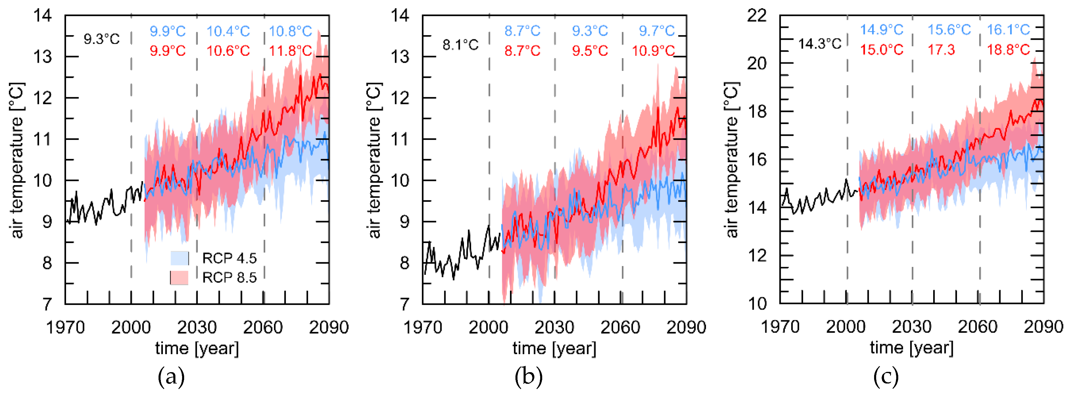
First, we analysed the predicted change in annual air temperatures for the three different cities based on the multi-model ensemble and two different RCPs. Figure 1 highlights the results of the multi-model ensemble for mean annual air temperatures for London, Luxembourg, and Rome. The future climate projections of the nested regional climate model approaches show increases of the mean annual air temperatures for all three cities and the two different RCPs. London shows a 30-year mean of 9.3 °C for the reference period. An increase of the mean annual air temperature of 1.5 °C until end of this century is predicted for RCP4.5 and 2.5 °C for RCP8.5 (Figure 1a), respectively. With 8.1 °C, the reference period in Luxembourg is more than one degree colder than London but the projected increases for the RCPs are in comparable range at 1.6 °C (RCP4.5) and 2.8 °C (RCP8.5) (Figure 1b). Rome shows the highest increase from the reference period 1979–2000 (14.3 °C) to 2061–2090, with 1.8 °C (RCP4.5) and 4.5 °C (RCP8.5) (Figure 1c). All differences between the reference period and the three different future time spans for the three cities and two RCPs were statistically significant (p < 0.001).
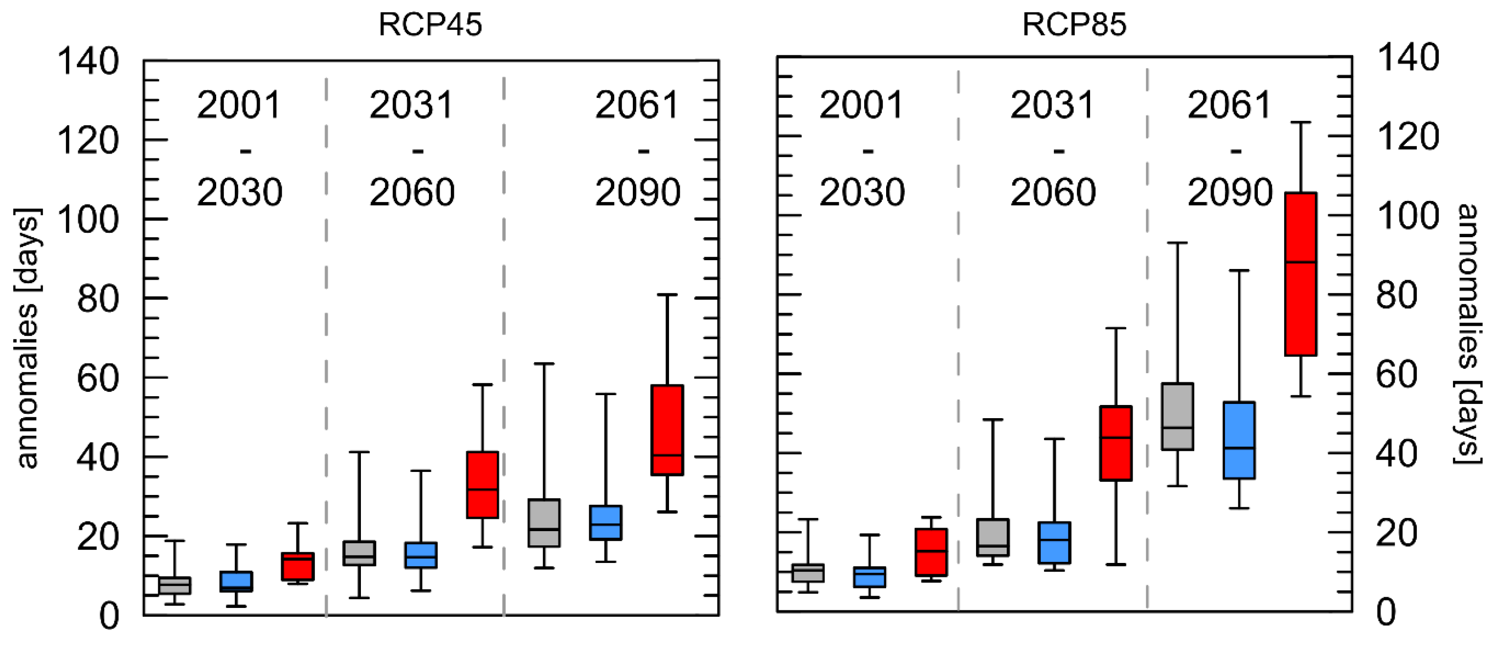
Figure 2 shows the boxplots of mean anomalies of the WSDI per year with reference to the 30-year period 1971–2000. The number of days contributing to events where the maximum air temperature is higher than the 90th percentile of the reference period on more than six consecutive days increases. Even though the mean annual air temperatures for London increases less in both RCPs than for Luxembourg, the corresponding WSDI exhibits stronger increases.
Comparing the anomalies between the cities, there are significant differences between London/Luxembourg (both RCPs) and Rome/Luxembourg, for the near future (2001–2030). For the middle (2031–2060) and far future (2061–2090) statistically significant differences could be observed for Rome/Luxembourg and London/Luxembourg for both RCPs. Especially for Rome, the mean of the WSDI increased from 51 to 105 days (please note that the box plots show median values and not the arithmetic means).
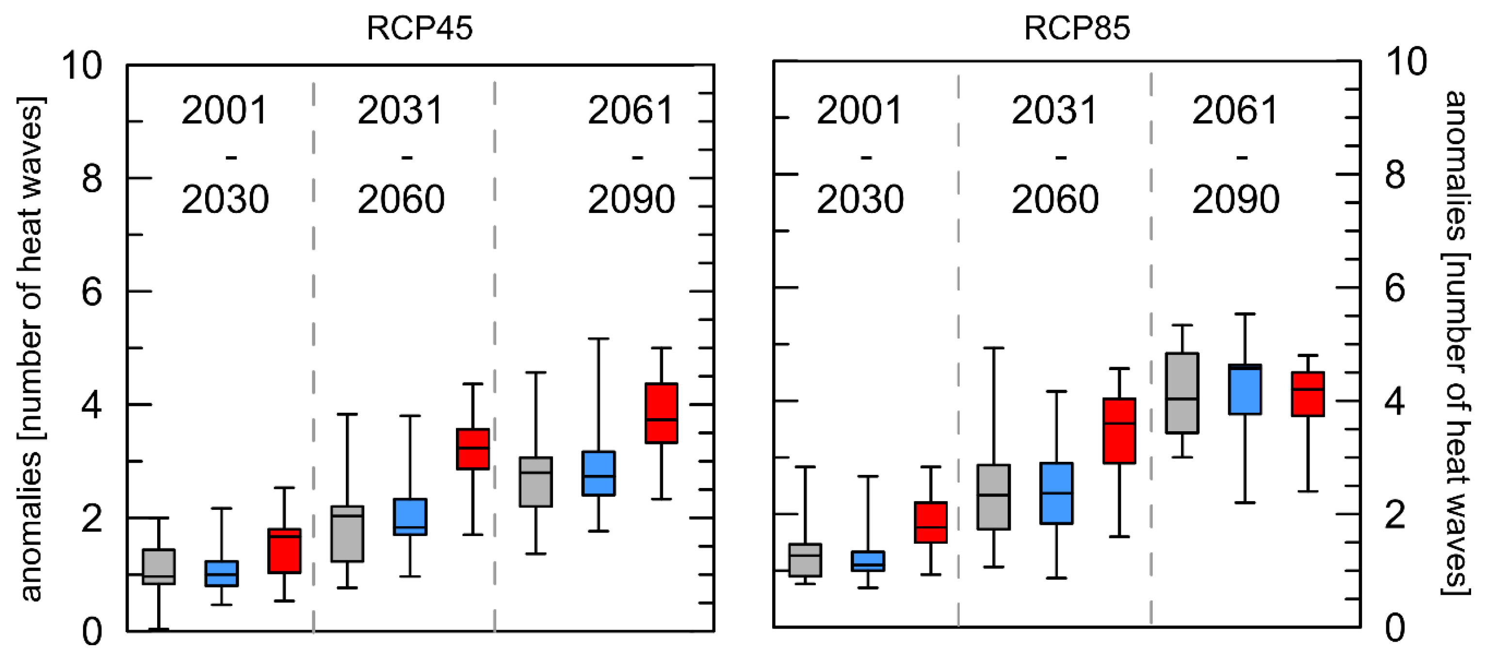
The following four indices are based on different definition of heat waves compared to the WSDI (description in Section 2.2). For the absolute number of HWs, all thirteen ensemble members show positive anomalies compared to their individual reference periods. The boxplots in Figure 3 illustrates that there are no big differences in the absolute number of HWs between RCP 4.5 and RCP 8.5. In both scenarios, there is an increase of one HW for London and Luxembourg for the near and two for the middle future. For the far future London and Luxembourg will have three more HWs for RCP 4.5 and four for RCP8.5.
Differences between the cities are not significant for the near future for RCP4.5 and for the far future for RCP8.5. For all other time spans significant differences could be observed between Rome/London as well as Rome/Luxembourg for both RCPs.
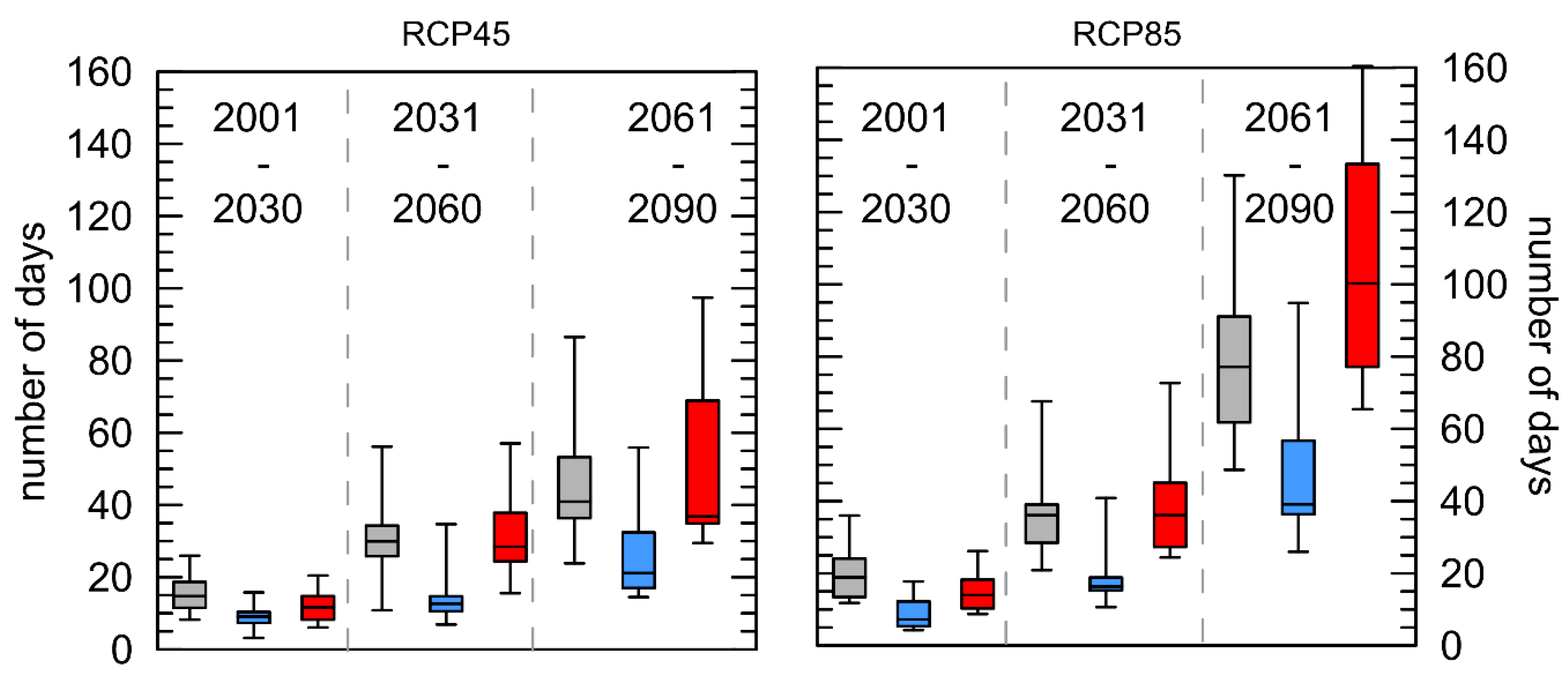
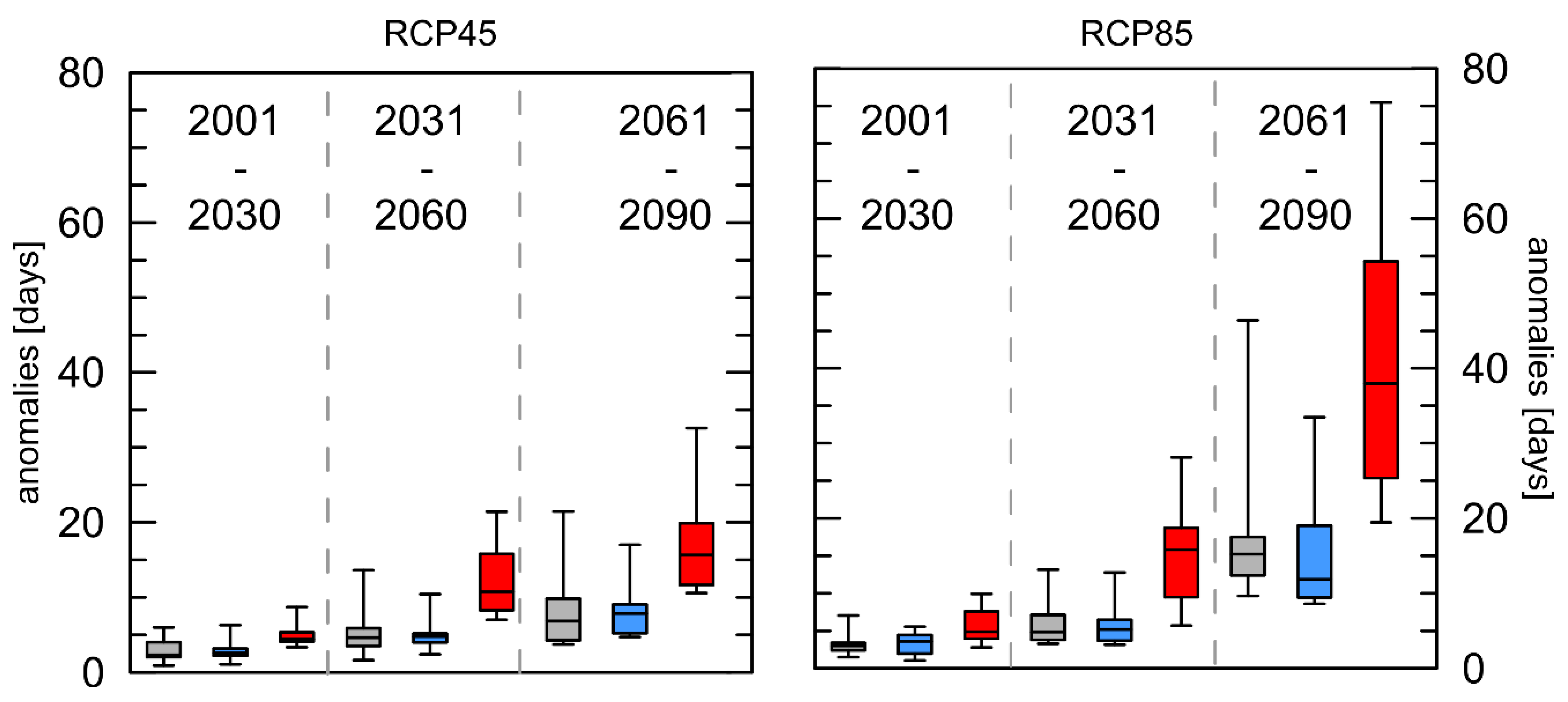
The number of days that contribute to the absolute number of HWs were analysed further (Figure 4). For both RCPs in the near future, only slight changes could be observed. Already in the middle future, differences become obvious between London and Luxembourg compared to Rome, and this effect is even more pronounced for the far future. The mean number of days that contribute to an HW in Rome amounts to 47 (RCP4.5) and 86 (RCP8.5) in the far future time span.
The statistical analysis of the differences between the cities showed that for all cases, the differences between Rome/London as well as Rome/Luxembourg are significant and, those between London/Luxembourg are not.
A more detailed analysis, strongly related to health impacts, looks at the length of extreme heat events. Therefore, the anomalies for the length of the longest heat wave per year are shown in Figure 5. Again, a similar pattern can be observed with a strong increase for the far future only for Rome for RCP8.5. For London and Luxembourg, in the near future for both RCPs a prolongation of approximately 3 days is calculated, and for the middle future 5 and 6 days, respectively. Once more, the strongest increase is observed for Rome with a prolongation of 18 days for RCP4.5 and 41 days for RCP8.5.
The comparison between the cities yields the same significant differences between for Rome/London and Rome/Luxembourg, while the London/Luxembourg differences are not significant.
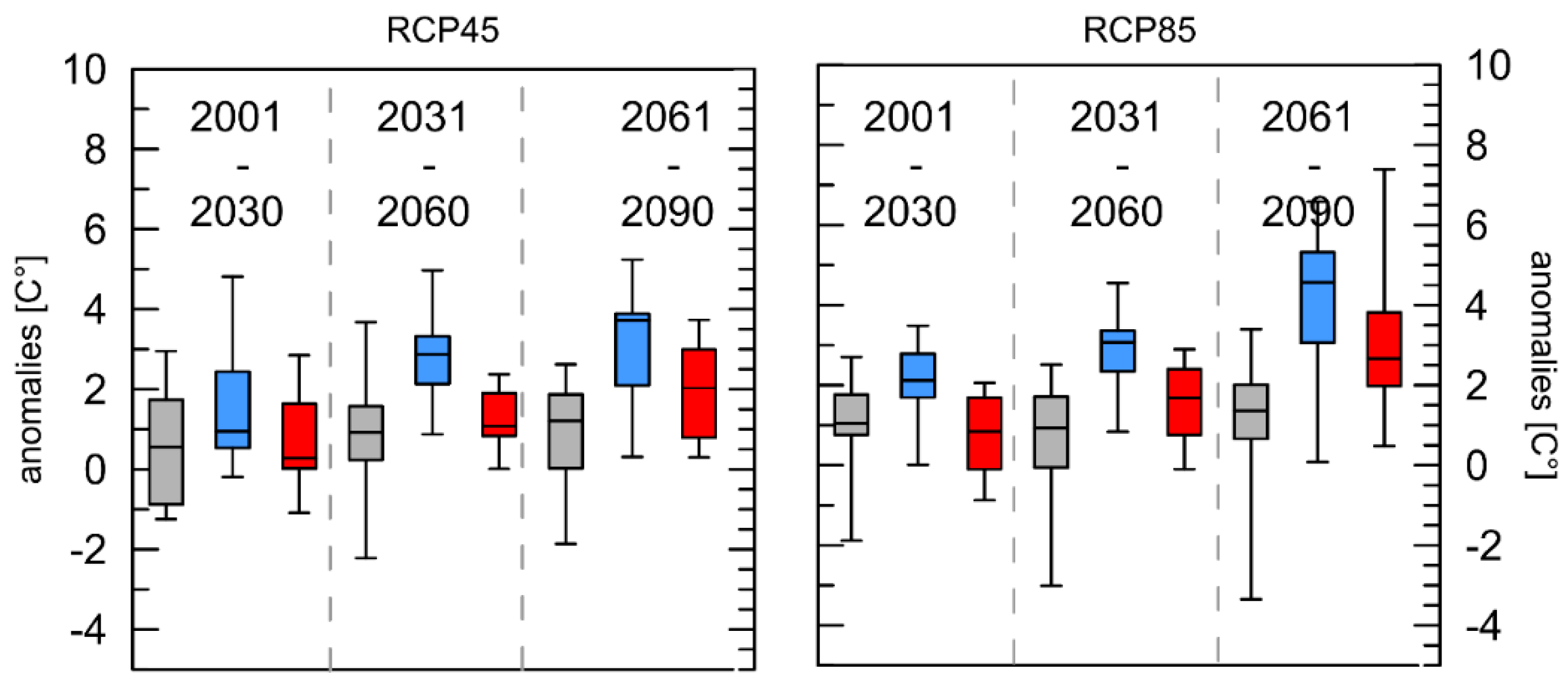
The last index describes the mean air temperature of all detected HWs per year (Figure 6). In contrast to the others indices, here the results are less homogeneous. Especially for London, some of the ensemble members project even slight negative anomalies. However, overall a general increase for both RCPs in the mean air temperature during the heat wave can be observed for all cities and all future time spans. The differences for near future of the RCP4.5 scenario are not significant, those for the far future of the same RCPs are. For the middle future, only the differences between Rome/Luxembourg and Rome/London are significant. For the RCP8.5 in the near future the differences between Luxembourg/Rome and Luxembourg/London are significant, for the middle future all differences, and for the far future, Luxembourg/London and London/Rome.
4. Discussion
Climate warming will directly impact the probability of the occurrence of future extreme events and, thus, negatively impact different sectors like agriculture, ecosystems and human health [6,22]. Unfortunately, there is no standardized universal definition of HWs, meaning that direct comparisons between reported results are sometimes complicated, but the overall definition describes HWs as time spans of consecutive days with hotter conditions than usual [14]. To contribute to the unification efforts of the World Meteorological Organisation (WMO), the indices defined by the Expert Team on Sector-specific Climate Indices (ET-SCI) were used in this study. In general, past heat waves are a well investigated phenomena, e.g., the Chicago HW from 1995 [23,24] or the Paris HW from 2003 [25,26,27]. For the assessment of future frequencies and intensities of HWs, climate change projections are useful tools to derive potential future risks [5,28,29,30,31].
In our analysis, we rely on a multi-physics and multi-model ensemble of different regional climate models forced with two different emission scenarios (RCP4.5 and RCP8.5.). No weighting of the individual model results was used. To reduce the noise of the results, averages of 30-year time spans were calculated and it was these results that were finally used for the statistical analysis [29].
The projected changes in air temperature for the three different cities shown in Figure 1 are in line with results from comparable studies for London [32], Luxembourg [33,34,35,36] and Rome [37,38]. For London, an increase in the long-term annual mean air temperature by 1.5 °C for the RCP4.5 and 2.5 °C for the RCP8.5 is projected. Past research demonstrated that there is a clear link between increased mortality and increased air temperature and HWs [12] and heat-related diseases like respiratory and cardiovascular illnesses [39]. In addition, there is a strong relationship between increased air temperatures and amplified near surface ozone concentrations that reinforce the negative health effects [40]. According to recent studies in England and Wales the mortality increases by 2.1% for each 1 °C increase in air temperature above the 95th percentile of the average yearly temperature [32,39,41]. With 1.6 °C and 2.8 °C the projected increase in air temperature is a bit more pronounced for Luxembourg. The consequences for the regional fauna and flora were analysed in different climate change impact studies in the past [34,35,36,42,43]. For Rome the highest anomalies of up to 4.5 °C were projected corresponding to results shown for the Mediterranean region [29].
The duration of the heat wave expressed as WSDI, shown in Figure 2, can be used as a measure for how long the population is exposed to high levels of heat stress. A continuous increase in the WSDI could be observed for all cities with the highest anomalies for Rome and RCP8.5, which is consistent with the trends in the mean annual air temperature shown in Figure 1. Long-term, continuous exposure to high ambient air temperatures—targeted by this index—during the nights can decrease sleep quality significantly [44] especially for older people [45]. The WSDI was already applied for the past climate worldwide based on the HadEX2 data set [46]. In Europe for the time span 1961–2010, positive trends between 2.3 and 2.9 days per decade [47] could be observed. The impacts of projected changes in air temperature based on that index were analysed e.g., for China [22], showing a statistically significant increase of 2.4 days per decade on average since 1961.
The index shown in Figure 3 comprises the absolute number of HWs per year (HW-N) and is strongly related to the index describing the number of days (Figure 4) that contribute to HWs per year (HW-F). The absolute number of days that contribute to HWs influences the number and the duration of the events but HW-F is not equal to HW-D multiplied with HW-N, because HW-D indicates the duration of the longest event, not the average duration [14].
Based on the “in the meantime updated SRES emission scenarios” an increase in the globally averaged (land only) number of HWs between 4 and 12 depending on the emission scenario was simulated [48]. Although there is not much difference in the number of heat waves between the two scenarios, the number of days’ contribution to heat waves each year with reference to the 30-year period 1971–2000 increases significantly following the projected general increase in air temperature. It is worth noticing, that the arithmetic mean of the HW-N anomalies for Rome in the RCP8.5 scenario for the far future is lower (+4.0 HW) than that for London (+4.1 HW) and Luxembourg (+4.2 HW) and additionally, the increase for the far future is less pronounced here than for the other indices. This could be explained by the fact that the increased number of days that contribute to HWs prolonged the length of the HWs substantially, so that few but very long HWs occur in all three cities every year at the end of this century. This is reconfirmed by the results presented in Figure 5. The HW-D index—describing the length of the longest HW per year—shows overall positive anomalies with the most pronounced positive trends for the far future. For both RCPs for Rome, the highest anomalies were projected for the far future. This index only describes the most extreme event per year, but is important for the health aspects because the longer the heat waves last, the more pronounced heat-related illnesses are. For Mumbai (India) an increase of one day in the duration of an HW was associated with a 4.9% increase in the estimated association between HWs and mortality [49]. The detected increase in the duration of heat waves in the future are similar to those presented for Eastern Europe or northern Russia [50].
Results of the analysis of the HW-M index also showed increases in the mean temperature during the HWs for all cities and RCPs, where Luxembourg showed the strongest increase (Figure 6). For England and Wales 1.0% of all summer deaths were attributable to air temperature [51], and an increase of 1 °C corresponded to a 3.1% increase in daily mortality. In Mediterranean cities a 2% increase in mortality is associated with a rise of approximately 10 °C [13].
Further research is necessary to analyse the timing of the HWs within a year, because HWs occurring earlier in the summer may have greater effects on mortality [52,53]. The importance of the age structure is highlighted by the 2003 HW in France. Beginning of August 2003 air temperatures were above 35 °C, and at some meteorological stations even above 40 °C [54]. More than 15,000 excess deaths were observed [55]. It was shown by [56] that mortality excess was estimated to 20% (age 45–74 years), 70% (age 75–94 year) and 120% (older than 94 years). This was also shown for other European countries by for different age classes [57].
Beside the effects of HWs on health they also might negatively influence food security and water supply, leading to higher incidence of water-borne infectious and toxin-related illnesses, such as cholera or bluetongue emergence [58,59]. Furthermore, HWs are of highly relevance for hydrological processes but also agriculture and forestry [60,61,62,63].
5. Conclusions
To understand projected changes in the frequency and intensity of HWs and their potential negative impacts on public health a detailed knowledge of the projected changes in air temperature distribution is fundamental [64]. A consistent increase in the frequency and intensity of HWs for the three selected cities was detected by the use of common climate change indices, recommended by the WMO and is in line with comparable results from different working groups [65,66,67]. Even if anthropogenic greenhouse gas emissions could be completely stopped, a continuous warming will take place over the next few decades.
The influence of elevated heat stress on public health has been demonstrated in past studies. A better understanding of the health risks and health impacts of extreme events, combined with the knowledge of the expected changes for dedicated cities, is a prerequisite for further steps. Beside the necessary mitigation efforts, that must be undertaken to limit climate warming to a minimum, increased resilience and the formulation of appropriate adaptation measures is crucial to reducing negative health impacts in the future. Additionally, a science-based prioritisation of urban planning measures, implementation of heat warning systems and other effective public health actions will be possible based on such analysis.
Author Contributions
J.J. designed the study, analysed the data, interpreted the results and drafted the manuscript. K.G. was responsible for the handling of the climate change projections, the time series data extraction and assisted in the preparation of the manuscript. A.K. helped in the interpretation of the results and assisted in the preparation of the manuscript.
Funding
This research was funded by the “Ministère de l’Environnement, du Climat et du Développement durable” of Luxembourg. The Horizon 2020 project eLTER (Integrated European Long-Term Ecosystem & Socio-Ecological Research Infrastructure - GA: 654359 - H2020 INFRAIA call 2014-2015) provided support to K. Goergen.
Acknowledgments
We acknowledge the World Climate Research Programme’s Working Group on Regional Climate, and the Working Group on Coupled Modelling, the former coordinating body of CORDEX and responsible panel for CMIP5. We also thank the climate modelling groups (listed in Table 1 of this paper) for producing and making available their model output. We also acknowledge the Earth System Grid Federation infrastructure, an international effort led by the U.S. Department of Energy’s Program for Climate Model Diagnosis and Intercomparison, the European Network for Earth System Modelling and other partners in the Global Organisation for Earth System Science Portals (GO-ESSP). We also thank U. Schulzweida for the freely available CDO tool, Version 1.9.6. Additionally, we acknowledge the work of the Expert Team on Sector-specific Climate Indices and the support of Lindsey Auguin for language editing.
Conflicts of Interest
The authors declare no conflict of interest.
References
- IPCC. Climate Change 2013: The Physical Science Basis. Contribution of Working Group I to the Fifth Assessment Report of the Intergovernmental Panel on Climate Change; Stocker, T.F., Qin, D., Plattner, G.-K., Tignor, M., Allen, S.K., Boschung, J., Nauels, A., Xia, Y., Bex, V., Midgley, P.M., Eds.; Cambridge University Press: Cambridge, UK; New York, NY, USA, 2013; p. 1535. [Google Scholar] [CrossRef]
- Field, C.B.; Barros, V.; Stocker, T.F.; Qin, D.; Dokken, D.J.; Ebi, K.L.; Mastrandrea, M.D.; Mach, K.J.; Plattner, G.K.; Allen, S.K.; et al. Managing the Risks of Extreme Events and Disasters to Advance Climate Change Adaptation. A Special Report of Working Groups I and II of the Intergovernmental Panel on Climate Change; Cambridge University Press: Cambridge, UK, 2012; p. 582. [Google Scholar]
- Van Oldenborgh, G.J.; Philip, S.; Kew, S.; Vautard, R.; Boucher, O.; Otto, F.; Haustein, K.; Soubeyroux, J.-M.; Ribes, A.; Robin, Y.; et al. Human Contribution to the Record-Breaking June 2019 Heat Wave in France; World Weather Attribution (WWA): Amsterdam, Netherlands, 2019; p. 32. [Google Scholar]
- Easterling, D.R.; Meehl, G.A.; Parmesan, C.; Changnon, S.A.; Karl, T.R.; Mearns, L.O. Climate Extremes: Observations, Modeling, and Impacts. Science 2000, 289, 7. [Google Scholar] [CrossRef] [PubMed]
- Mann, M.E.; Rahmstorf, S.; Kornhuber, K.; Steinman, B.A.; Miller, S.K.; Petri, S.; Coumou, D. Projected changes in persistent extreme summer weather events: The role of quasi-resonant amplification. Sci. Adv. 2018, 4, 9. [Google Scholar] [CrossRef] [PubMed]
- IPCC. Climate Change 2007: The Physical Science Basis: Contribution of Working Group I to the Fourth Assessment Report of the Intergovernmental Panel on Climate Change; Cambridge University Press: Cambridge, UK, 2007. [Google Scholar]
- Watts, N.; Amann, M.; Arnell, N.; Ayeb-Karlsson, S.; Belesova, K.; Berry, H.; Bouley, T.; Boykoff, M.; Byass, P.; Cai, W.; et al. The 2018 report of the Lancet Countdown on health and climate change: Shaping the health of nations for centuries to come. Lancet 2018, 392, 2479–2514. [Google Scholar] [CrossRef]
- Orimoloye, I.R.; Mazinyo, S.P.; Kalumba, A.M.; Ekundayo, O.Y.; Nel, W. Implications of climate variability and change on urban and human health: A review. Cities 2019, 91, 213–223. [Google Scholar] [CrossRef]
- Jendritzky, G.; Tinz, B. The thermal environment of the human being on the global scale. Glob. Health Action 2009, 2. [Google Scholar] [CrossRef] [PubMed]
- Sahu, S.; Sett, M.; Kjellstrom, T. Heat Exposure, Cardiovascular Stress and Work Productivity in Rice Harvesters in India: Implications for a Climate Change Future. Ind. Health 2013, 51, 424–431. [Google Scholar] [CrossRef] [Green Version]
- Lokys, H.L.; Junk, J.; Krein, A. Short-term effects of air quality and thermal stress on non-accidental morbidity—A multivariate meta-analysis comparing indices to single measures. Int. J. Biometeorol. 2018, 62, 17–27. [Google Scholar] [CrossRef]
- Ropo, O.I.; Perez, M.S.; Werner, N.; Enoch, I.T. Climate Variability and Heat Stress Index have Increasing Potential Ill-health and Environmental Impacts in the East London, South Africa. Int. J. Appl. Eng. Res. 2017, 12, 6910–6918. [Google Scholar]
- Basu, R.; Samet, J.M. Relation between elevated ambient temperature and mortality: A review of the epidemiologic evidence. Epidemiol. Rev. 2002, 24, 190–202. [Google Scholar] [CrossRef]
- Perkins, S.E.; Alexander, L.V. On the Measurement of Heat Waves. J. Clim. 2013, 26, 4500–4517. [Google Scholar] [CrossRef]
- Cinquini, L.; Crichton, D.; Mattmann, C.; Harney, J.; Shipman, G.; Wang, F.; Ananthakrishnan, R.; Miller, N.; Denvil, S.; Morgan, M.; et al. The Earth System Grid Federation: An open infrastructure for access to distributed geospatial data. Future Gener. Comput. Syst. 2014, 36, 400–417. [Google Scholar] [CrossRef]
- Jacob, D.; Petersen, J.; Eggert, B.; Alias, A.; Christensen, O.B.; Bouwer, L.M.; Braun, A.; Colette, A.; Déqué, M.; Georgievski, G.; et al. EURO-CORDEX: New high-resolution climate change projections for European impact research. Reg. Environ. Chang. 2014, 14, 563–578. [Google Scholar] [CrossRef]
- Taylor, K.E.; Stouffer, R.J.; Meehl, G.A. An Overview of CMIP5 and the Experiment Design. Bull. Am. Meteorol. Soc. 2012, 93, 485–498. [Google Scholar] [CrossRef] [Green Version]
- Moss, R.H.; Edmonds, J.A.; Hibbard, K.A.; Manning, M.R.; Rose, S.K.; van Vuuren, D.P.; Carter, T.R.; Emori, S.; Kainuma, M.; Kram, T.; et al. The next generation of scenarios for climate change research and assessment. Nature 2010, 463, 747. [Google Scholar] [CrossRef] [PubMed]
- Kotlarski, S.; Keuler, K.; Christensen, O.B.; Colette, A.; Déqué, M.; Gobiet, A.; Goergen, K.; Jacob, D.; Lüthi, D.; van Meijgaard, E.; et al. Regional climate modeling on European scales: A joint standard evaluation of the EURO-CORDEX RCM ensemble. Geosci. Model Dev. 2014, 7, 1297–1333. [Google Scholar] [CrossRef]
- Prein, A.F.; Gobiet, A.; Truhetz, H.; Keuler, K.; Goergen, K.; Teichmann, C.; Fox Maule, C.; van Meijgaard, E.; Déqué, M.; Nikulin, G.; et al. Precipitation in the EURO-CORDEX 0.11° and 0.44° simulations: High resolution, high benefits? Clim. Dyn. 2016, 46, 383–412. [Google Scholar] [CrossRef]
- Maraun, D. Bias Correcting Climate Change Simulations—A Critical Review. Curr. Clim. Chang. Rep. 2016, 2, 211–220. [Google Scholar] [CrossRef]
- Yin, H.; Sun, Y. Characteristics of extreme temperature and precipitation in China in 2017 based on ETCCDI indices. Adv. Clim. Chang. Res. 2018, 9, 218–226. [Google Scholar] [CrossRef]
- Karl, T.R.; Knight, R.W. The 1995 Chicago Heat Wave: How Likely Is a Recurrence? Bull. Am. Meteorol. Soc. 1997, 78, 1107–1120. [Google Scholar] [CrossRef]
- Kaiser, R.; Le Tertre, A.; Schwartz, J.; Gotway, C.A.; Randolph, W.; Rubin, C.H. The Effect of the 1995 Heat Wave in Chicago on All-Cause and Cause-Specific Mortality. Am. J. Public Health 2007, 97, 158–162. [Google Scholar] [CrossRef]
- Schär, C.; Vidale, P.L.; Lüthi, D.; Frei, C.; Häberli, C.; Liniger, M.A.; Appenzeller, C. The role of increasing temperature variability in European summer heatwaves. Nature 2004, 427, 332–336. [Google Scholar] [CrossRef] [PubMed]
- Laaidi, K.; Zeghnoun, A.; Dousset, B.; Bretin, P.; Vandentorren, S.; Giraudet, E.; Beaudeau, P. The impact of heat islands on mortality in Paris during the August 2003 heat wave. Environ. Health Perspect. 2012, 120, 254–259. [Google Scholar] [CrossRef] [PubMed]
- Christidis, N.; Jones, G.S.; Stott, P.A. Dramatically increasing chance of extremely hot summers since the 2003 European heatwave. Nat. Clim. Chang. 2014, 5, 46. [Google Scholar] [CrossRef]
- Cammarano, D.; Tian, D. The effects of projected climate and climate extremes on a winter and summer crop in the southeast USA. Agric. For. Meteorol. 2018, 248, 109–118. [Google Scholar] [CrossRef]
- Meehl, G.A.; Tebaldi, C. More Intense, More Frequent, and Longer Lasting Heat Waves in the 21st Century. Science 2004, 305, 4. [Google Scholar] [CrossRef]
- Nastos, P.T.; Kapsomenakis, J. Regional climate model simulations of extreme air temperature in Greece. Abnormal or common records in the future climate? Atmos. Res. 2015, 152, 43–60. [Google Scholar] [CrossRef]
- Perkins, S.E.; Alexander, L.V.; Nairn, J.R. Increasing frequency, intensity and duration of observed global heatwaves and warm spells. Geophys. Res. Lett. 2012, 39. [Google Scholar] [CrossRef]
- Paavola, J. Health impacts of climate change and health and social inequalities in the UK. Environ. Health 2017, 16, 113. [Google Scholar] [CrossRef]
- Goergen, K.; Beersma, J.; Hoffmann, L.; Junk, J. ENSEMBLES-based assessment of regional climate effects in Luxembourg and their impact on vegetation. Clim. Chang. 2013, 119, 761–773. [Google Scholar] [CrossRef]
- Junk, J.; Kouadio, L.; Delfosse, P.; El Jarroudi, M. Effects of regional climate change on brown rust disease in winter wheat. Clim. Chang. 2016, 135, 439–451. [Google Scholar] [CrossRef] [Green Version]
- Lokys, H.L.; Junk, J.; Krein, A. Future Changes in Human-Biometeorological Index Classes in Three Regions of Luxembourg, Western-Central Europe. Adv. Meteorol. 2015, 2015, 10. [Google Scholar] [CrossRef] [PubMed]
- Junk, J.; Ulber, B.; Vidal, S.; Eickermann, M. Assessing climate change impacts on the rape stem weevil, Ceutorhynchus napi Gyll., based on bias- and non-bias-corrected regional climate change projections. Int. J. Biometeorol. 2015, 59, 1597–1605. [Google Scholar] [CrossRef] [PubMed]
- Picarelli, L.; Comegna, L.; Gariano, S.L.; Guzzetti, F.; Rianna, G.; Santini, M.; Tommasi, P. Potential climate changes in italy and consequences for land stability. In Slope Safety Preparedness for Impact of Climate Change; CRC Press: Boca Raton, FL, USA, 2017; pp. 151–198. [Google Scholar] [CrossRef]
- Chelli, S.; Wellstein, C.; Campetella, G.; Canullo, R.; Tonin, R.; Zerbe, S.; Gerdol, R. Climate change response of vegetation across climatic zones in Italy. Clim. Res. 2017, 71, 249–262. [Google Scholar] [CrossRef]
- Hajat, S.; Vardoulakis, S.; Heaviside, C.; Eggen, B. Climate change effects on human health: Projections of temperature-related mortality for the UK during the 2020s, 2050s and 2080s. J. Epidemiol. Community Health 2014, 68, 641–648. [Google Scholar] [CrossRef] [PubMed]
- Filleul, L.; Cassadou, S.; Medina, S.; Fabres, P.; Lefranc, A.; Eilstein, D.; Le Tertre, A.; Pascal, L.; Chardon, B.; Blanchard, M.; et al. The relation between temperature, ozone, and mortality in nine French cities during the heat wave of 2003. Environ. Health Perspect. 2006, 114, 1344–1347. [Google Scholar] [CrossRef] [PubMed]
- Johnson, H.; Kovats, S.; McGregor, G.; Stedman, J.; Gibbs, M.; Walton, H. The impact of the 2003 heat wave on daily mortality in England and Wales and the use of rapid weekly mortality estimates. Eurosurveillance 2005, 10, 15–16. [Google Scholar] [CrossRef]
- Molitor, D.; Junk, J. Climate change is implicating a two-fold impact on air temperature increase in the ripening period under the conditions of the Luxembourgish grapegrowing region. OENO One 2019, 53. [Google Scholar] [CrossRef]
- Molitor, D.; Caffarra, A.; Sinigoj, P.; Pertot, I.; Hoffmann, L.; Junk, J. Late frost damage risk for viticulture under future climate conditions: A case study for the Luxembourgish winegrowing region. Aust. J. Grape Wine Res. 2014, 20, 160–168. [Google Scholar] [CrossRef]
- Lan, L.; Tsuzuki, K.; Liu, Y.F.; Lian, Z.W. Thermal environment and sleep quality: A review. Energy Build. 2017, 149, 101–113. [Google Scholar] [CrossRef]
- Okamoto-Mizuno, K.; Tsuzuki, K.; Mizuno, K. Effects of mild heat exposure on sleep stages and body temperature in older men. Int. J. Biometeorol. 2004, 49, 32–36. [Google Scholar] [CrossRef]
- Donat, M.G.; Alexander, L.V.; Yang, H.; Durre, I.; Vose, R.; Dunn, R.J.H.; Willett, K.M.; Aguilar, E.; Brunet, M.; Caesar, J.; et al. Updated analyses of temperature and precipitation extreme indices since the beginning of the twentieth century: The HadEX2 dataset. J. Geophys. Res. Atmos. 2013, 118, 2098–2118. [Google Scholar] [CrossRef]
- Christidis, N.; Stott, P.A. Attribution analyses of temperature extremes using a set of 16 indices. Weather Clim. Extrem. 2016, 14, 24–35. [Google Scholar] [CrossRef] [Green Version]
- Tebaldi, C.; Hayhoe, K.; Arblaster, J.M.; Meehl, G.A. Going to the Extremes. Clim. Chang. 2006, 79, 185–211. [Google Scholar] [CrossRef]
- Nori-Sarma, A.; Anderson, G.B.; Rajiva, A.; ShahAzhar, G.; Gupta, P.; Pednekar, M.S.; Son, J.Y.; Peng, R.D.; Bell, M.L. The impact of heat waves on mortality in Northwest India. Environ. Res. 2019, 176, 108546. [Google Scholar] [CrossRef] [PubMed]
- Lavaysse, C.; Cammalleri, C.; Dosio, A.; van der Schrier, G.; Toreti, A.; Vogt, J. Towards a monitoring system of temperature extremes in Europe. Nat. Hazards Earth Syst. Sci. 2018, 18, 91–104. [Google Scholar] [CrossRef] [Green Version]
- Arbuthnott, K.G.; Hajat, S. The health effects of hotter summers and heat waves in the population of the United Kingdom: A review of the evidence. Environ. Health 2017, 16, 119. [Google Scholar] [CrossRef] [PubMed]
- Montero, J.C.; Mirón, I.J.; Criado-Álvarez, J.J.; Linares, C.; Díaz, J. Influence of local factors in the relationship between mortality and heat waves: Castile-La Mancha (1975–2003). Sci. Total Environ. 2012, 414, 73–80. [Google Scholar] [CrossRef]
- Rocklov, J.; Barnett, A.; Woodward, A. On the estimation of heat-intensity and heat-duration effects in time series models of temperature-related mortality in Stockholm, Sweden. Environ. Health 2012, 11–23. [Google Scholar] [CrossRef]
- Astrom, D.O.; Forsberg, B.; Rocklov, J. Heat wave impact on morbidity and mortality in the elderly population: A review of recent studies. Maturitas 2011, 69, 99–105. [Google Scholar] [CrossRef]
- Fouillet, A.; Rey, G.; Laurent, F.; Pavillon, G.; Bellec, S.; Guihenneuc-Jouyaux, C.; Clavel, J.; Jougla, E.; Hémon, D. Excess mortality related to the August 2003 heat wave in France. Int. Arch. Occup. Environ. Health 2006, 80, 16–24. [Google Scholar] [CrossRef] [Green Version]
- Pirard, P.; Vandentorren, S.; Pascal, M.; Laaidi, K.; Le Tertre, A.; Cassadou, S.; Ledrans, M. Summary of the mortality impact assessment of the 2003 heat wave in France. Euro Surveill. Bull. Eur. Mal. Transm. Eur. Commun. Dis. Bull. 2005, 10, 153–156. [Google Scholar] [CrossRef]
- Kosatsky, T. The 2003 European heat waves. Eurosurveillance 2005, 10. [Google Scholar] [CrossRef] [PubMed]
- Patz, J.A.; Epstein, P.R.; Burke, T.A.; Balbus, J.M. Global Climate Change and Emerging Infectious Diseases. JAMA 1996, 275, 217–223. [Google Scholar] [CrossRef] [PubMed]
- Caminade, C.; McIntyre, K.M.; Jones, A.E. Impact of recent and future climate change on vector-borne diseases. Ann. N. Y. Acad. Sci. 2019, 1436, 157–173. [Google Scholar] [CrossRef]
- Terzago, S.; von Hardenberg, J.; Palazzi, E.; Provenzale, A. Snow water equivalent in the Alps as seen by gridded data sets, CMIP5 and CORDEX climate models. Cryosphere 2017, 11, 1625–1645. [Google Scholar] [CrossRef] [Green Version]
- Verfaillie, D.; Lafaysse, M.; Déqué, M.; Eckert, N.; Lejeune, Y.; Morin, S. Multi-component ensembles of future meteorological and natural snow conditions for 1500m altitude in the Chartreuse mountain range, Northern French Alps. Cryosphere 2018, 12, 1249–1271. [Google Scholar] [CrossRef]
- Frei, P.; Kotlarski, S.; Liniger, M.A.; Schär, C. Future snowfall in the Alps: Projections based on the EURO-CORDEX regional climate models. Cryosphere 2018, 12, 1–24. [Google Scholar] [CrossRef]
- Hanzer, F.; Förster, K.; Nemec, J.; Strasser, U. Projected cryospheric and hydrological impacts of 21st century climate change in the Ötztal Alps (Austria) simulated using a physically based approach. Hydrol. Earth Syst. Sci. 2018, 22, 1593–1614. [Google Scholar] [CrossRef]
- Lewis, S.C.; King, A.D. Evolution of mean, variance and extremes in 21st century temperatures. Weather Clim. Extrem. 2017, 15, 1–10. [Google Scholar] [CrossRef]
- Russo, S.; Dosio, A.; Graversen, R.G.; Sillmann, J.; Carrao, H.; Dunbar, M.B.; Singleton, A.; Montagna, P.; Barbola, P.; Vogt, J.V. Magnitude of extreme heat waves in present climate and their projection in a warming world. J. Geophys. Res. Atmos. 2014, 119, 12500–12512. [Google Scholar] [CrossRef]
- Dosio, A.; Mentaschi, L.; Fischer, E.M.; Wyser, K. Extreme heat waves under 1.5 °C and 2 °C global warming. Environ. Res. Lett. 2018, 13. [Google Scholar] [CrossRef]
- Smid, M.; Russo, S.; Costa, A.C.; Granell, C.; Pebesma, E. Ranking European capitals by exposure to heat waves and cold waves. Urban Clim. 2019, 27, 388–402. [Google Scholar] [CrossRef]
Figure 1.
Multi-model ensemble of mean annual air temperature values for London (a), Luxembourg (b), and Rome (c) based on two different Representative Concentration Pathways (RCPs) (4.5 = blue; 8.5 = red). Spread is defined via +/− one standard deviation of the ensemble. Please note that the scale of Figure 1c is different from a and b.

Figure 2.
Boxplots of mean anomalies of the “Warm spell duration indicator” (WSDI) per year with reference to the 30-year period 1971–2000 for the three cities London (grey), Luxembourg (blue), and Rome (red) and two different RCPs. Whiskers = 5/95 percentile.
Figure 2.
Boxplots of mean anomalies of the “Warm spell duration indicator” (WSDI) per year with reference to the 30-year period 1971–2000 for the three cities London (grey), Luxembourg (blue), and Rome (red) and two different RCPs. Whiskers = 5/95 percentile.

Figure 3.
Boxplots of mean anomalies of the number of heat waves per year (HW-N) with reference to the 30-year period 1971–2000 for the three cities London (grey), Luxembourg (blue), and Rome (red) and two different RCPs. Whiskers = 5/95 percentile.
Figure 3.
Boxplots of mean anomalies of the number of heat waves per year (HW-N) with reference to the 30-year period 1971–2000 for the three cities London (grey), Luxembourg (blue), and Rome (red) and two different RCPs. Whiskers = 5/95 percentile.

Figure 4.
Boxplots of mean anomalies of the number of days’ contribution to heat waves each year (HW-F) with reference to the 30-year period 1971–2000 for the three cities London (grey), Luxembourg (blue), and Rome (red) and two different RCPs. Whiskers = 5/95 percentile.
Figure 4.
Boxplots of mean anomalies of the number of days’ contribution to heat waves each year (HW-F) with reference to the 30-year period 1971–2000 for the three cities London (grey), Luxembourg (blue), and Rome (red) and two different RCPs. Whiskers = 5/95 percentile.

Figure 5.
Boxplots of mean anomalies of the length of the longest heat waves each year (HW-D) with reference to the 30-year period 1971–2000 for the three cities London (grey), Luxembourg (blue), and Rome (red) and two different RCPs. Whiskers = 5/95 percentile.
Figure 5.
Boxplots of mean anomalies of the length of the longest heat waves each year (HW-D) with reference to the 30-year period 1971–2000 for the three cities London (grey), Luxembourg (blue), and Rome (red) and two different RCPs. Whiskers = 5/95 percentile.

Figure 6.
Boxplots of mean anomalies of the mean temperature of all heat waves per year (HW-M) with reference to the 30-year period 1971–2000 for the three cities London (grey), Luxembourg (blue), and Rome (red) and two different RCPs. Whiskers = 5/95 percentile.
Figure 6.
Boxplots of mean anomalies of the mean temperature of all heat waves per year (HW-M) with reference to the 30-year period 1971–2000 for the three cities London (grey), Luxembourg (blue), and Rome (red) and two different RCPs. Whiskers = 5/95 percentile.


Table 1.
Regional climate change projection datasets used in the study. The table contain the model abbreviations used in the text, the driving Global Climate Model (GCM), the Regional Climate Model (RCM) used for the dynamical downscaling as well as the institutions that are responsible for the model runs; temporal resolution: daily data; time span: 1971–2091.
| Model Number | Official CMIP5 GCM Name | Modelling Centre/Group CMIP5 “Institute ID” | Official EURO-CORDEX RCM Name | Modelling Centre/Group EURO-CORDEX “Institute ID” |
|---|---|---|---|---|
| M01 | CNRM-CM5 | CNRM-CERFACS | ALADIN53 | CNRM |
| M02 | CNRM-CM5 | CNRM-CERFACS | ALARO-0 | RMIB-UGent |
| M05 | MPI-ESM-LR | MPI-M | REMO2009 | MPI-CSC |
| M06 | MPI-ESM-LR | MPI-M | RCA4 | SMHI |
| M07 | NorESM1-M | NCC | HIRHAM5 | DMI |
| M09 | HadGEM2-ES | CNRM MOHC | RCA4 | SMHI |
| M10 | IPSL-CM5A-MR | IPSL | WRF331F | IPSL-INERIS |
| M11 | CNRM-CM5 | CNRM-CERFACS | CCLM4-8-17 | CLMcom |
| M12 | EC-EARTH | ICHEC | RACMO22E | KNMI |
| M13 | IPSL-CM5A-MR | IPSL | RCA4 | SMHI |
| M14 | MPI-ESM-LR | MPI-M | CCLM4-8-17 | CLMcom |
Table 2.
Definition of extreme temperature indices according to ClimPact2.
| Abbreviation | Definition | Unit |
|---|---|---|
| HW-D | Length of longest HW | days |
| HW-F | Number of days that contribute to heat waves | days |
| HW-M | Mean temperature of all heat wave in a year | °C |
| HW-N | Number of heat waves per year | number |
| WSDI | Number of days contributing to events where on > 6 consecutive days the maximum air temperature is in > 90th percentile | days |
© 2019 by the authors. Licensee MDPI, Basel, Switzerland. This article is an open access article distributed under the terms and conditions of the Creative Commons Attribution (CC BY) license (http://creativecommons.org/licenses/by/4.0/).
Share and Cite
MDPI and ACS Style
Junk, J.; Goergen, K.; Krein, A. Future Heat Waves in Different European Capitals Based on Climate Change Indicators. Int. J. Environ. Res. Public Health 2019, 16, 3959. https://doi.org/10.3390/ijerph16203959
AMA Style
Junk J, Goergen K, Krein A. Future Heat Waves in Different European Capitals Based on Climate Change Indicators. International Journal of Environmental Research and Public Health. 2019; 16(20):3959. https://doi.org/10.3390/ijerph16203959
Chicago/Turabian StyleJunk, Jürgen, Klaus Goergen, and Andreas Krein. 2019. "Future Heat Waves in Different European Capitals Based on Climate Change Indicators" International Journal of Environmental Research and Public Health 16, no. 20: 3959. https://doi.org/10.3390/ijerph16203959
Note that from the first issue of 2016, this journal uses article numbers instead of page numbers. See further details here.