Space-Time Statistical Insights about Geographic Variation in Lung Cancer Incidence Rates: Florida, USA, 2000–2011


Abstract
:1. Introduction
2. Background
3. Data and Methodology
3.1. Lung Cancer Incidence Rates
3.2. Moran Eigenvector Spatial Filtering
4. Results and Discussion
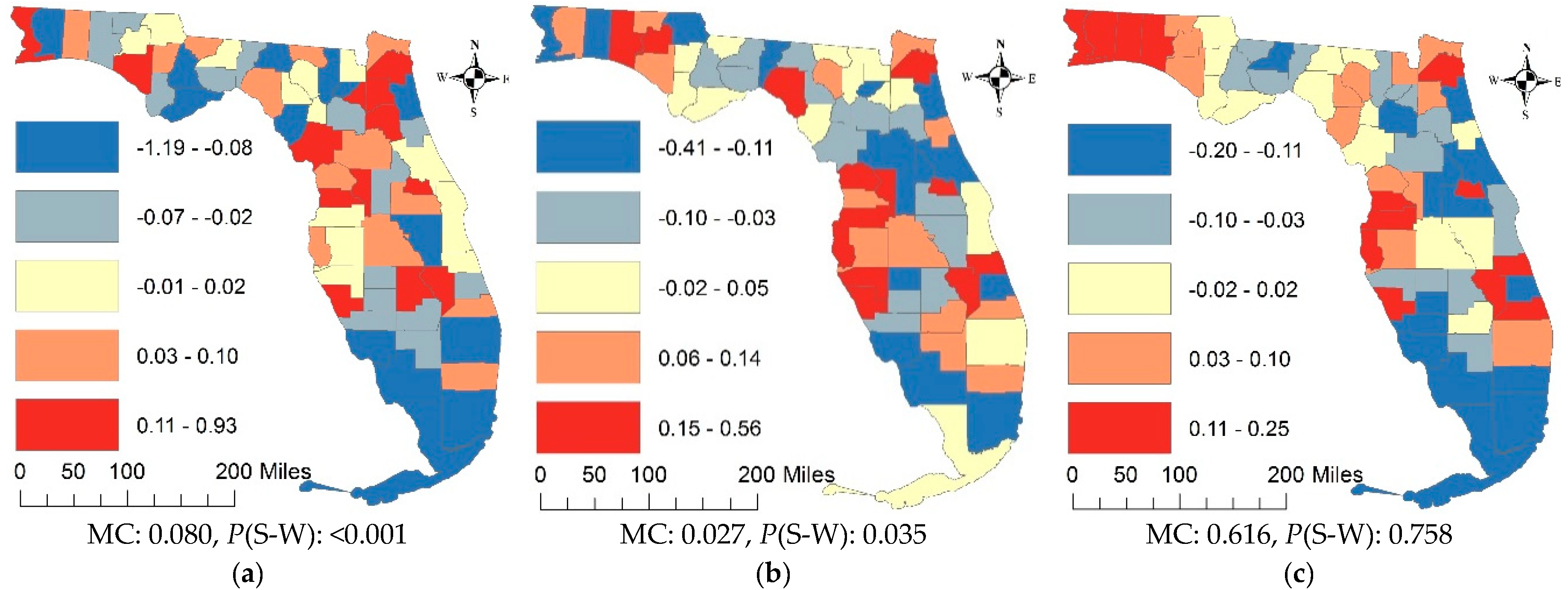
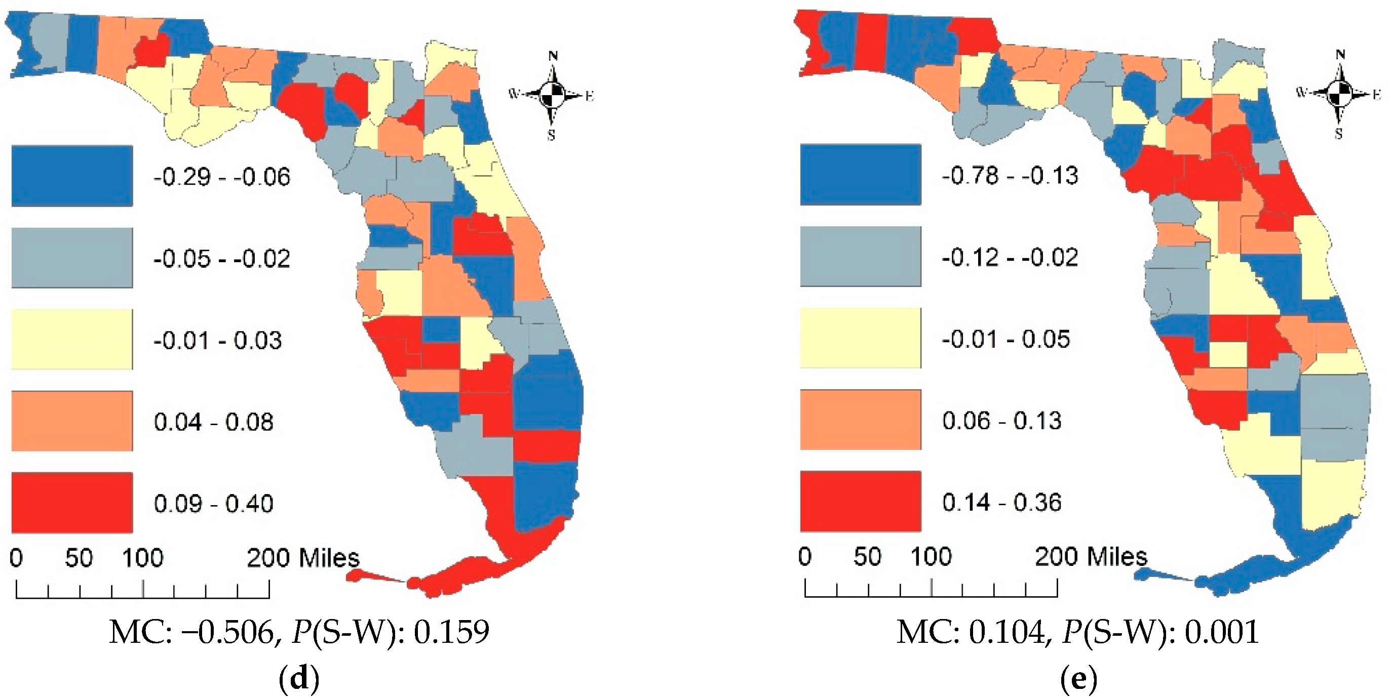
4.1. The State Scale and County Resolution
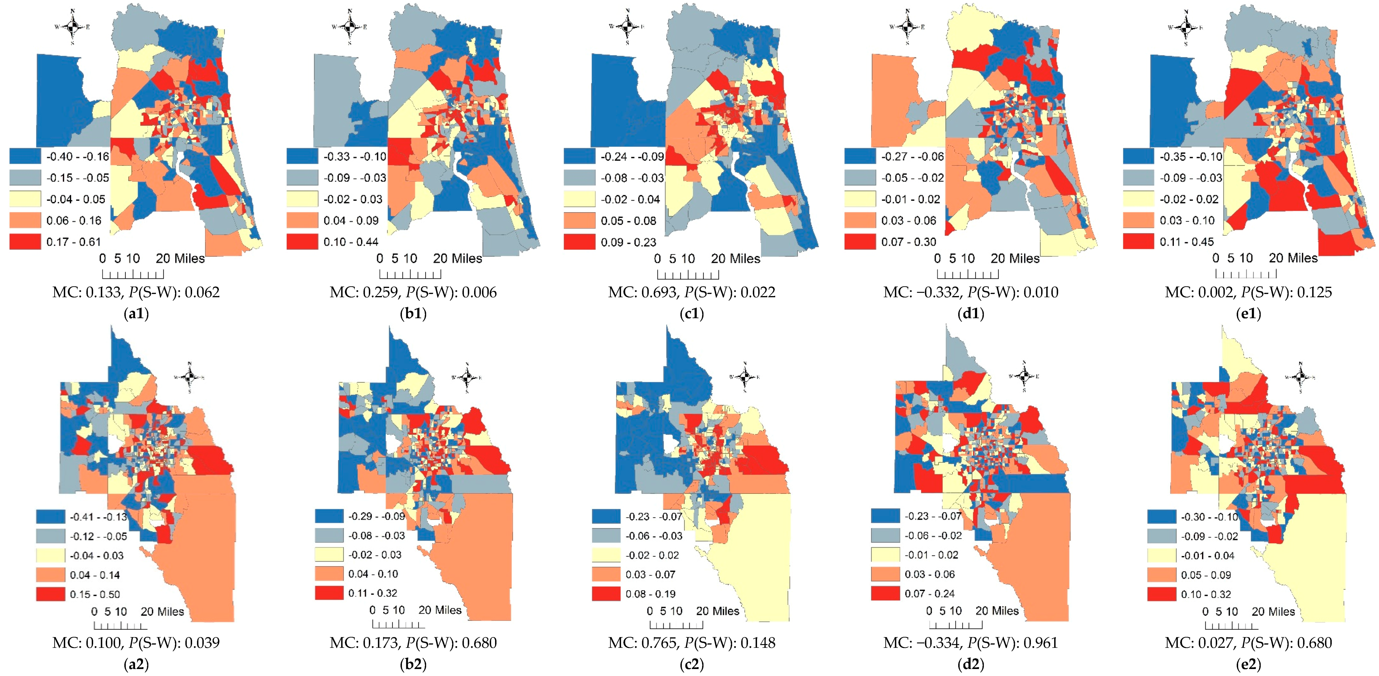
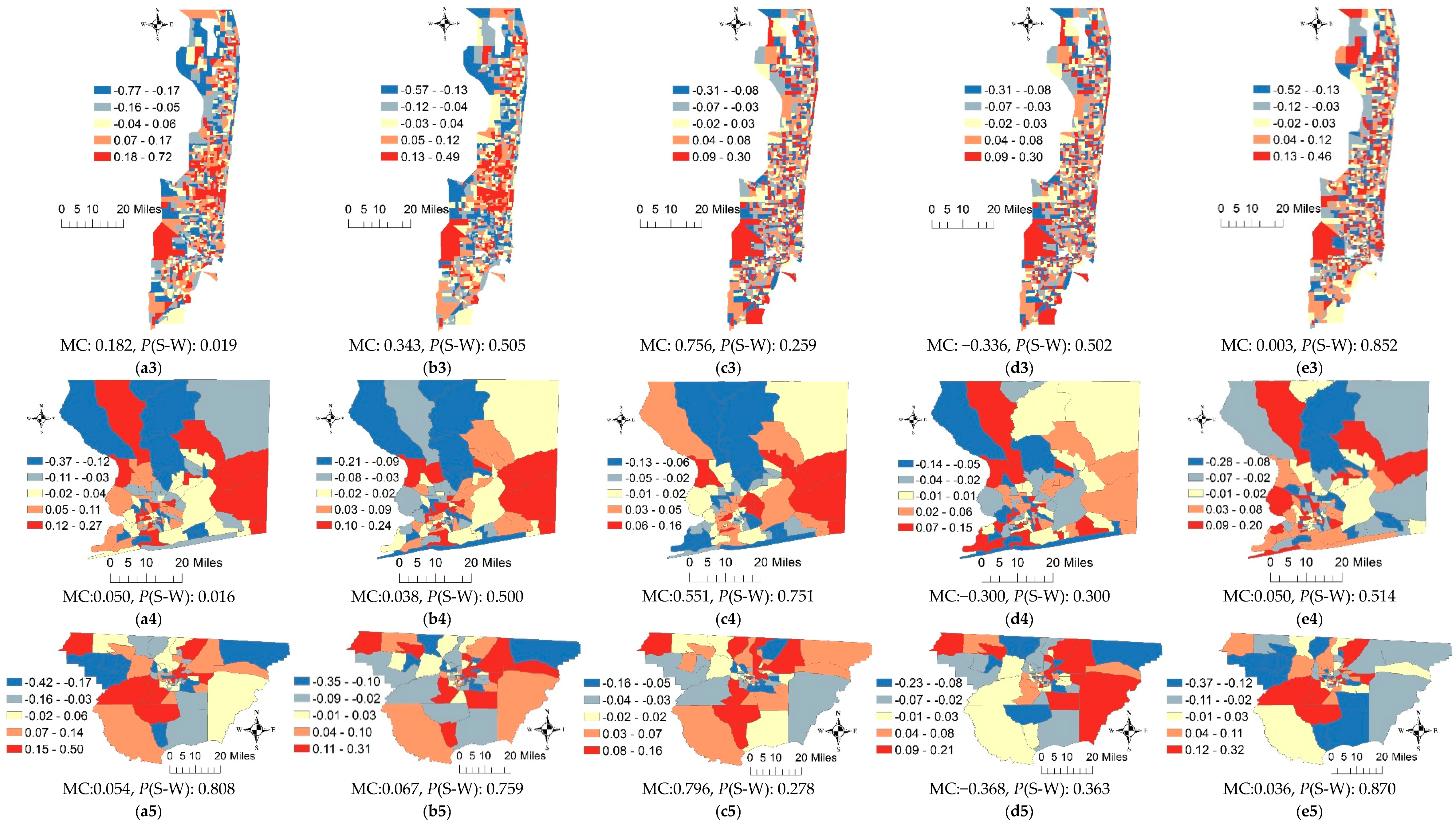
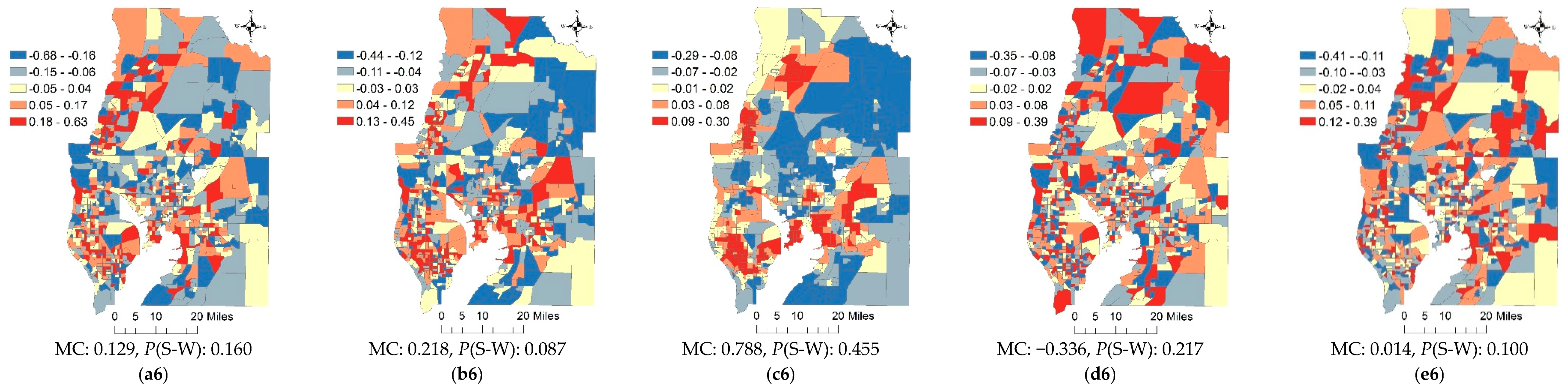
4.2. The Metropolitan Statistical Area Scale and Census Tract Resolution
5. Conclusions
Author Contributions
Funding
Conflicts of Interest
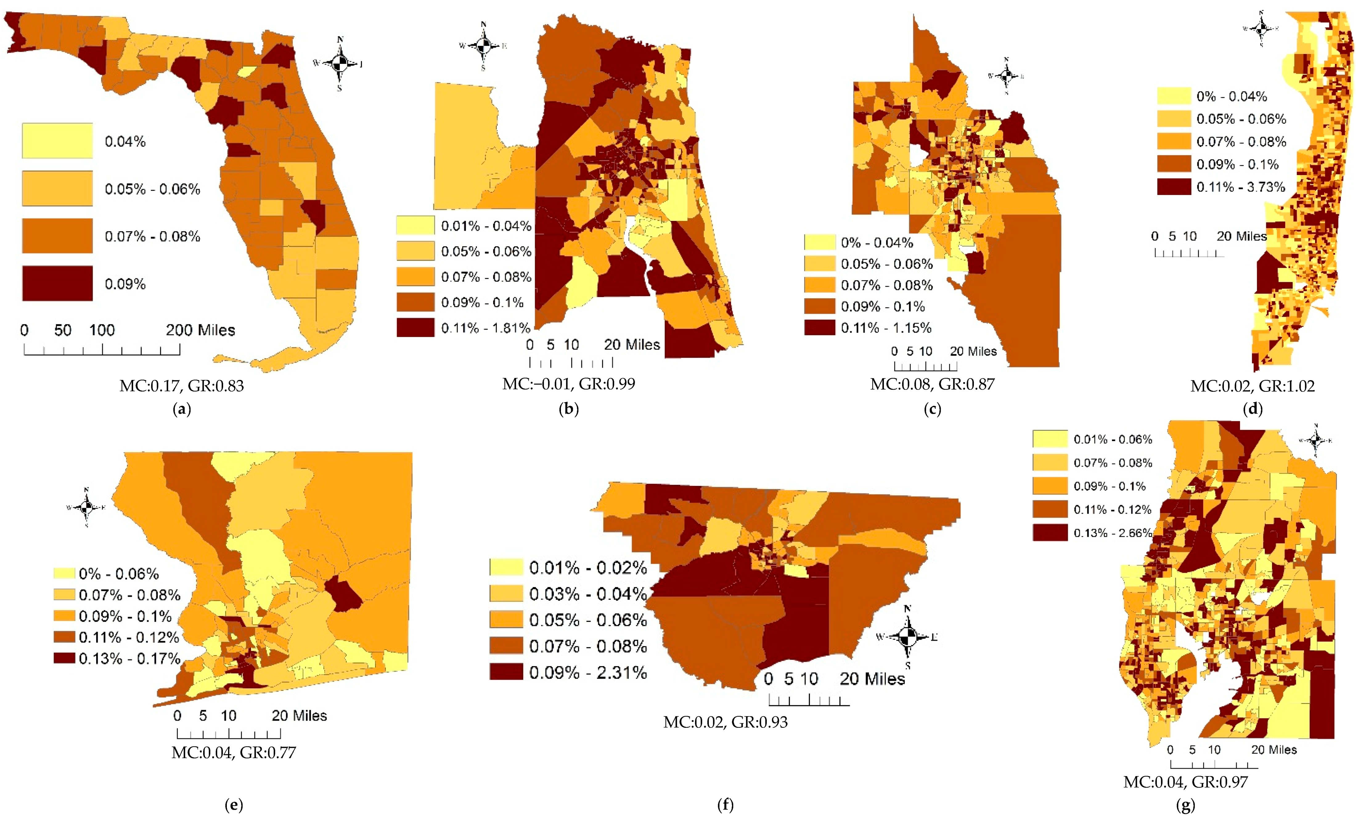
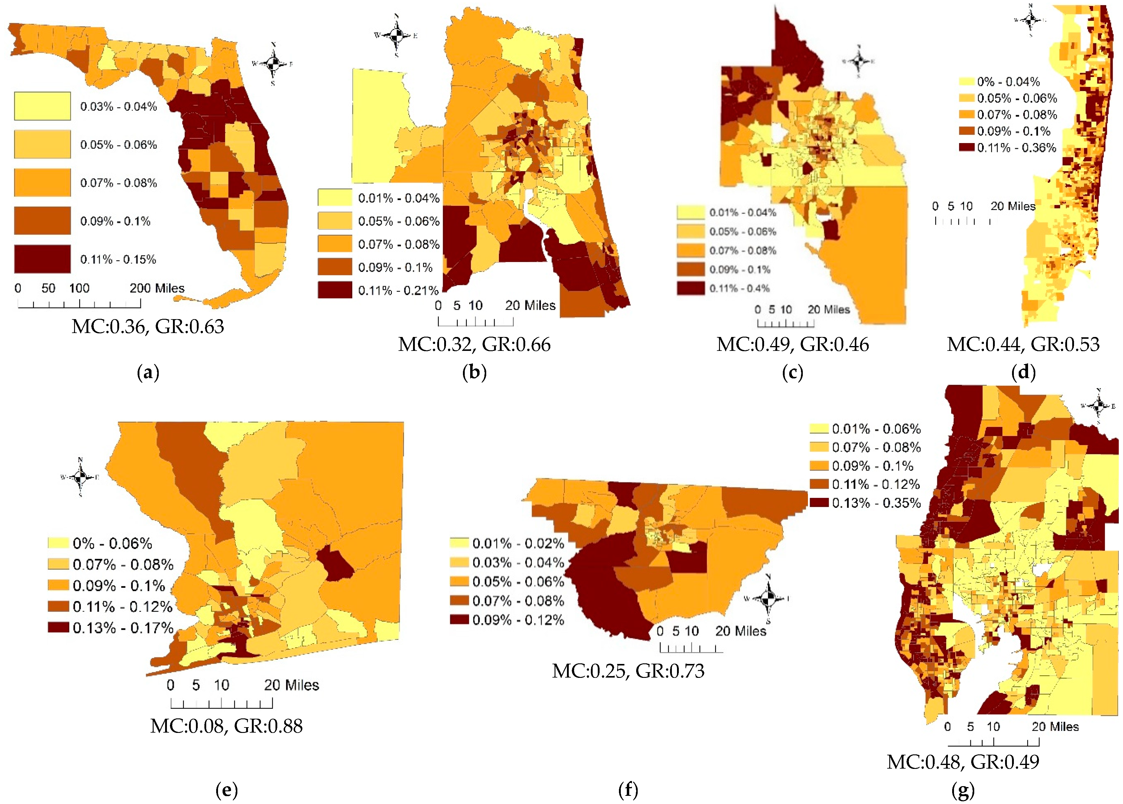
Appendix A. Crude Lung Cancer Incidence Rates Maps

References
- d’Onofrio, A.; Mazzetta, C.; Robertson, C.; Smans, M.; Boyle, P.; Boniol, M. Maps and atlases of cancer mortality: A review of a useful tool to trigger new questions. Ecancermedicalscience 2016, 10, 670. [Google Scholar] [CrossRef] [PubMed]
- Wieland, S.; Cassa, C.; Mandl, K.; Berger, B. Revealing the spatial distribution of a disease while preserving privacy. Proc. Natl. Acad. Sci. USA 2008, 105, 17608–17613. [Google Scholar] [CrossRef] [PubMed] [Green Version]
- Lee, M.; Chun, Y.; Griffith, D. An evaluation of kernel smoothing to protect confidentiality of patient locations. Int. J. Urban Sci. 2018, in press. [Google Scholar] [CrossRef]
- Smith, H.; Seal, S.; Sullivan, D. Impact of race, poverty, insurance coverage and resource availability on breast cancer across geographic regions of Mississippi. J. Miss. Acad. Sci. 2017, 62, 353–369. [Google Scholar] [CrossRef]
- Roquette, R.; Nunes, B.; Painho, M. The relevance of spatial aggregation level and of applied methods in the analysis of geographical distribution of cancer mortality in mainland Portugal (2009–2013). Popul. Health Metr. 2018, 16, 6. [Google Scholar] [CrossRef] [PubMed] [Green Version]
- Wang, N.; Mengersen, K.; Kimlin, M.; Zhou, M.; Tong, S.; Fang, L.; Wang, B.; Hu, W. Lung cancer and particulate pollution: A critical review of spatial and temporal analysis evidence. Environ. Res. 2018, 164, 585–596. [Google Scholar] [CrossRef] [PubMed]
- Besag, J.; York, J.; Mollié, A. Bayesian image restoration, with two applications in spatial statistics. Ann. Inst. Stat. Math. 1991, 43, 1–20. [Google Scholar] [CrossRef]
- Griffth, D.; Arbia, G. Detecting negative spatial autocorrelation in georeferenced random variables. Int. J. Geogr. Inf. Sci. 2010, 24, 417–437. [Google Scholar] [CrossRef]
- Fukuda, Y.; Umezaki, M.; Nakamura, K.; Takano, T. Variations in societal characteristics of spatial disease clusters: Examples of colon, lung and breast cancer in Japan. Int. J. Health Geogr. 2005, 4, 16. [Google Scholar] [CrossRef] [PubMed] [Green Version]
- Mao, Y.; Hu, J.; Ugnat, A.; Semenciw, R.; Fincham, S. Socioeconomic status and lung cancer risk in Canada. Int. J. Epidemiol. 2001, 30, 809–817. [Google Scholar] [CrossRef] [PubMed] [Green Version]
- MacLennan, R.; Da Costa, J.; Day, N.; Law, C.; Ng, Y.; Shanmugaratnam, K. Risk factors for lung cancer in Singapore Chinese, a population with high female incidence rates. Int. J. Cancer 1977, 20, 854–860. [Google Scholar] [CrossRef] [PubMed]
- Molina, J.; Yang, P.; Cassivi, S.; Schild, S.; Adjei, A.A. Non-small cell lung cancer: Epidemiology, risk factors, treatment, and survivorship. In Mayo Clinic Proceedings; Elsevier: Amsterdam, The Netherlands, 2008; Volume 83, pp. 584–594. [Google Scholar]
- Alberg, A.; Samet, J.M. Epidemiology of lung cancer. Chest 2003, 123, 21S–49S. [Google Scholar] [CrossRef] [PubMed]
- Feskanich, D.; Ziegler, R.; Michaud, D.; Giovannucci, E.; Speizer, F.; Willett, W.; Colditz, G.A. Prospective study of fruit and vegetable consumption and risk of lung cancer among men and women. J. Natl. Cancer Inst. 2000, 92, 1812–1823. [Google Scholar] [CrossRef] [PubMed]
- Pope, C.A., III; Burnett, R.; Thun, M.; Calle, E.; Krewski, D.; Ito, K.; Thurston, G.D. Lung cancer, cardiopulmonary mortality, and long-term exposure to fine particulate air pollution. JAMA 2002, 287, 1132–1141. [Google Scholar] [CrossRef] [PubMed]
- Vineis, P.; Forastiere, F.; Hoek, G.; Lipsett, M. Outdoor air pollution and lung cancer: Recent epidemiologic evidence. Int. J. Cancer 2004, 111, 647–652. [Google Scholar] [CrossRef] [PubMed] [Green Version]
- Osler, M. Social class and health behavior in Danish adults: A longitudinal study. Public Health 1993, 107, 251–260. [Google Scholar] [CrossRef]
- Pomerleau, J.; Pederson, L.; Østbye, T.; Speechley, M.; Speechley, K.N. Health behaviours and socio-economic status in Ontario, Canada. Eur. J. Epidemiol. 1997, 13, 613–622. [Google Scholar] [CrossRef] [PubMed]
- Alberg, A.; Brock, M.; Samet, J.M. Epidemiology of lung cancer: Looking to the future. J. Clin. Oncol. 2005, 23, 3175–3185. [Google Scholar] [CrossRef] [PubMed]
- Haiman, C.; Stram, D.; Wilkens, L.; Pike, M.; Kolonel, L.; Henderson, B.; Le Marchand, L. Ethnic and racial differences in the smoking-related risk of lung cancer. N. Engl. J. Med. 2006, 354, 333–342. [Google Scholar] [CrossRef] [PubMed]
- Risch, H.A.; Howe, G.R.; Jain, M.; Burch, J.D.; Holowaty, E.J.; Miller, A.B. Are female smokers at higher risk for lung cancer than male smokers? A case-control analysis by histologic type. Am. J. Epidemiol. 1993, 138, 281–293. [Google Scholar] [CrossRef] [PubMed]
- Zang, E.A.; Wynder, E.L. Differences in lung cancer risk between men and women: Examination of the evidence. J. Natl. Cancer Inst. 1996, 88, 183–192. [Google Scholar] [CrossRef] [PubMed]
- Singh, G.; Miller, B.A. Health, life expectancy, and mortality patterns among immigrant populations in the United States. Can. J. Public Health 2004, 95, 14–21. [Google Scholar]
- Blue, L.; Fenelon, A. Explaining low mortality among US immigrants relative to native-born Americans: The role of smoking. Int. J. Epidemiol. 2011, 40, 786–793. [Google Scholar] [CrossRef] [PubMed]
- Bosdriesz, J.; Lichthart, N.; Witvliet, M.; Busschers, W.; Stronks, K.; Kunst, A.E. Smoking prevalence among migrants in the US compared to the US-born and the population in countries of origin. PLoS ONE 2013, 8, e58654. [Google Scholar] [CrossRef] [PubMed]
- Jacquez, G.; Greiling, D.A. Geographic boundaries in breast, lung and colorectal cancers in relation to exposure to air toxics in Long Island, New York. Int. J. Health Geogr. 2003, 2, 4. [Google Scholar] [CrossRef] [PubMed]
- Kelsall, J.; Diggle, P.J. Spatial variation in risk of disease: A nonparametric binary regression approach. J. R. Stat. Soc. Ser. C Appl. Stat. 1998, 47, 559–573. [Google Scholar] [CrossRef]
- Richardson, S.; Abellan, J.; Best, N. Bayesian spatio-temporal analysis of joint patterns of male and female lung cancer risks in Yorkshire (UK). Stat. Methods Med. Res. 2006, 15, 385–407. [Google Scholar] [CrossRef] [PubMed]
- Jerrett, M.; Burnett, R.; Ma, R.; Pope, C.A., III; Krewski, D.; Newbold, K.; Thurston, G.; Shi, Y.; Finkelstein, N.; Calle, E.E.; et al. Spatial analysis of air pollution and mortality in Los Angeles. Epidemiology 2005, 16, 727–736. [Google Scholar] [CrossRef] [PubMed]
- Jin, X.; Carlin, B.; Banerjee, S. Generalized hierarchical multivariate CAR models for areal data. Biometrics 2005, 61, 950–961. [Google Scholar] [CrossRef] [PubMed]
- Verbeke, G.; Molenberghs, G.; Rizopoulos, D. Random effects models for longitudinal data. In Longitudinal Research with Latent Variables; Springer: Berlin/Heidelberg, Germany, 2010; pp. 37–96. [Google Scholar]
- Frondel, M.; Vance, C. Fixed, random, or something in between. A variant of Hausman’s specification test for panel data estimators. Econ. Lett. 2010, 107, 327–329. [Google Scholar] [CrossRef]
- Clarke, P.; Crawford, C.; Steele, F.; Vignoles, A.F. The Choice between Fixed and Random Effects Models: Some Considerations for Educational Research; Russell Sage Foundation: New York, NY, USA, 2010. [Google Scholar]
- Chen, E.; Tarko, A.P. Modeling safety of highway work zones with random parameters and random effects models. Anal. Methods Accid. Res. 2014, 1, 86–95. [Google Scholar] [CrossRef]
- Anderson, R.; Rosenberg, H.M. Age standardization of death rates: Implementation of the year 2000 standard. Natl. Vital Stat. Rep. 1998, 47, 1–17. [Google Scholar] [PubMed]
- Ahmad, O.; Boschi-Pinto, C.; Lopez, A.; Murray, C.; Lozano, R.; Inoue, M. Age Standardization of Rates: A New WHO Standard; World Health Organization: Geneva, Switzerland, 2010; Volume 9. [Google Scholar]
- Griffith, D.A. Spatial Autocorrelation and Spatial Filtering: Gaining Understanding through Theory and Scientific Visualization; Springer: Berlin, Germany, 2003. [Google Scholar]
- Chun, Y.; Griffith, D.; Lee, M.; Sinha, P. Eigenvector selection with stepwise regression techniques to construct eigenvector spatial filters. J. Geogr. Syst. 2016, 18, 67–85. [Google Scholar] [CrossRef]
- Griffith, D. Estimating missing data values for georeferenced Poisson counts. Geogr. Anal. 2013, 45, 259–284. [Google Scholar] [CrossRef]
- Griffith, D.A. Hidden negative spatial autocorrelation. J. Geogr. Syst. 2006, 8, 335–355. [Google Scholar] [CrossRef]
- O’brien, R.M. A caution regarding rules of thumb for variance inflation factors. Qual. Quant. 2007, 41, 673–690. [Google Scholar] [CrossRef]
- Craney, T.; Surles, J.G. Model-dependent variance inflation factor cutoff values. Qual. Eng. 2002, 14, 391–403. [Google Scholar] [CrossRef]
- Ward, E.; Jemal, A.; Cokkinides, V.; Singh, G.; Cardinez, C.; Ghafoor, A.; Thun, M. Cancer disparities by race/ethnicity and socioeconomic status. CA Cancer J. Clin. 2004, 54, 78–93. [Google Scholar] [CrossRef] [PubMed]
- Clegg, L.; Reichman, M.; Miller, B.; Hankey, B.; Singh, G.; Lin, Y.; Goodman, M.T.; Lynch, C.F.; Schwartz, S.M.; Chen, V.W.; et al. Impact of socioeconomic status on cancer incidence and stage at diagnosis: Selected findings from the surveillance, epidemiology, and end results: National Longitudinal Mortality Study. Cancer Causes Control 2009, 20, 417–435. [Google Scholar] [CrossRef] [PubMed]
- Stellman, S.; Chen, Y.; Muscat, J.; Djordjevic, I.; Richie, J.R.; Lazarus, P.; Thompson, S.; Altorki, N.; Berwick, M.; Citron, M.L.; et al. Lung cancer risk in white and black Americans. Ann. Epidemiol. 2003, 13, 294–302. [Google Scholar] [CrossRef]
- Muscat, J.; Richie, J.; Stellman, S.D. Mentholated cigarettes and smoking habits in whites and blacks. Tob. Control 2002, 11, 368–371. [Google Scholar] [CrossRef] [PubMed] [Green Version]
- Diggle, P.; Milne, R.K. Negative binomial quadrat counts and point processes. Scand. J. Stat. 1983, 10, 257–267. [Google Scholar]
- Openshaw, S. The modifiable areal unit problem. In Concepts and Techniques in Modern Geography; Study Group in Quantitative Methods of the Institute of British Geographers: Norwich, UK, 1984. [Google Scholar]
- Bentham, G. Migration and morbidity: Implications for geographical studies of disease. Soc. Sci. Med. 1988, 26, 49–54. [Google Scholar] [CrossRef]
- Boyle, P.; Norman, P.; Rees, P. Does migration exaggerate the relationship between deprivation and limiting long-term illness? A Scottish analysis. Soc. Sci. Med. 2002, 55, 21–31. [Google Scholar] [CrossRef]
- Hughes, A.E. Residential Mobility and CRC Screening: A Spatial Analysis of CRC Screening in an Urban Safety-Net Clinic; The University of Texas at Dallas: Dallas, TX, USA, 2016. [Google Scholar]


| Variables | Quasi-Poisson Model | Poisson Random Effects Model | ||||||
|---|---|---|---|---|---|---|---|---|
| Coeff. | Std. Error | VIF | Coeff. | Std. Error | Cor. † | |||
| Smoking | 4.060 | *** | 0.317 | 2.158 | 1.355 | * | 0.994 | <0.001 |
| Income | −0.262 | 0.262 | 2.763 | 0.191 | 0.617 | −0.034 | ||
| Education | −0.983 | * | 0.443 | 4.150 | 1.116 | 0.928 | <0.001 | |
| Poverty | −4.368 | *** | 1.027 | 7.584 | 1.608 | 2.191 | <0.001 | |
| Hispanic pop | −0.027 | 0.161 | 4.738 | 0.051 | 0.074 | 0.074 | ||
| Black pop | 1.587 | *** | 0.284 | 6.005 | −0.627 | 0.427 | 0.067 | |
| Immigrants | −0.015 | 0.013 | 2.449 | 0.033 | 0.050 | 0.021 | ||
| Overdispersion | 13.02 | 2.12 | ||||||
| Pseudo-R2 | 0.30 | 0.75 | ||||||
| Variables | Pensacola MSA | Tallahassee MSA | Jacksonville MSA | Orlando MSA | Miami MSA | Tampa MSA | ||||||||||||||||||
|---|---|---|---|---|---|---|---|---|---|---|---|---|---|---|---|---|---|---|---|---|---|---|---|---|
| Coeff. | Std. Error | Vif | Coeff. | Std. Error | Vif | Coeff. | Std. Error | Vif | Coeff. | Std. Error | Vif | Coeff. | Std. Error | Vif | Coeff. | Std. Error | Vif | |||||||
| Income | −1.10 | *** | 0.19 | 3.25 | −0.91 | ** | 0.17 | 2.68 | −0.80 | *** | 0.09 | 2.46 | −0.73 | *** | 0.07 | 1.75 | −0.40 | *** | 0.03 | 1.75 | −0.58 | *** | 0.05 | 1.77 |
| Education | −0.62 | 0.33 | 2.80 | 0.43 | 0.40 | 2.32 | −0.86 | *** | 0.20 | 2.56 | −0.44 | * | 0.20 | 2.47 | −0.35 | *** | 0.09 | 4.00 | −0.56 | *** | 0.12 | 2.29 | ||
| Poverty | 0.85 | ** | 0.31 | 3.15 | 0.94 | * | 0.37 | 3.15 | 0.12 | 0.19 | 2.66 | 1.23 | *** | 0.19 | 2.18 | 0.01 | 0.10 | 2.54 | 0.54 | *** | 0.11 | 2.24 | ||
| Hispanic pop | 0.96 | 0.72 | 1.14 | −0.68 | 0.54 | 1.14 | 0.81 | *** | 0.24 | 1.11 | −0.58 | *** | 0.07 | 1.39 | −0.51 | *** | 0.03 | 2.22 | −0.17 | *** | 0.06 | 1.44 | ||
| Black pop | −0.55 | *** | 0.13 | 2.56 | −0.72 | *** | 0.16 | 2.15 | −0.19 | *** | 0.06 | 2.10 | −0.30 | *** | 0.07 | 1.95 | −0.19 | *** | 0.03 | 1.92 | −0.08 | 0.05 | 1.50 | |
| Immigrants | −6.61 | * | 3.12 | 1.16 | −2.69 | 4.29 | 1.28 | −3.07 | 1.60 | 1.06 | −9.15 | *** | 1.32 | 1.29 | 10.21 | *** | 1.29 | 1.11 | −6.06 | ** | 1.86 | 1.21 | ||
| Overdispersion | 1.08 | 1.16 | 1.26 | 1.22 | 1.27 | 1.30 | ||||||||||||||||||
| Pseudo-R2 | 0.14 | 0.17 | 0.17 | 0.40 | 0.43 | 0.36 | ||||||||||||||||||
| Variables | Pensacola MSA | Tallahassee MSA | Jacksonville MSA | Orlando MSA | Miami MSA | Tampa MSA | ||||||||||||||||||
|---|---|---|---|---|---|---|---|---|---|---|---|---|---|---|---|---|---|---|---|---|---|---|---|---|
| Coeff. | Std. Error | Cor. † | Coeff. | Std. Error | Cor. † | Coeff. | Std. Error | Cor. † | Coeff. | Std. Error | Cor. † | Coeff. | Std. Error | Cor. † | Coeff. | Std. Error | Cor. † | |||||||
| Income | −1.06 | *** | 0.27 | 0.02 | −0.99 | *** | 0.23 | 0.08 | −0.78 | *** | 0.12 | <0.01 | −0.79 | *** | 0.10 | −0.02 | −0.41 | *** | 0.05 | <0.01 | −0.65 | *** | −0.65 | −0.04 |
| Education | −0.79 | * | 0.48 | 0.01 | 0.53 | 0.56 | −0.05 | −0.86 | *** | 0.31 | <0.01 | −0.48 | * | 0.28 | 0.01 | −0.47 | *** | 0.14 | <0.01 | −0.66 | *** | −0.66 | <0.01 | |
| Poverty | 0.73 | 0.46 | −0.01 | 0.91 | 0.48 | −0.07 | 0.17 | 0.28 | −0.01 | 1.02 | *** | 0.27 | 0.01 | 0.06 | 0.15 | <0.01 | 0.30 | * | 0.30 | 0.05 | ||||
| Hispanic pop | 0.44 | 1.02 | 0.01 | −0.61 | 0.79 | 0.10 | 0.86 | *** | 0.37 | <0.01 | −0.69 | *** | 0.10 | 0.01 | −0.58 | *** | 0.04 | <0.01 | −0.17 | *** | −0.17 | −0.02 | ||
| Black pop | −0.50 | *** | 0.20 | −0.01 | −0.69 | *** | 0.22 | −0.04 | −0.17 | *** | 0.09 | <0.01 | −0.31 | *** | 0.10 | <0.01 | −0.27 | *** | 0.05 | <0.01 | −0.03 | −0.03 | −0.02 | |
| Immigrants | −7.82 | * | 4.52 | 0.02 | −4.91 | 5.80 | −0.05 | −2.86 | 2.58 | <0.01 | −9.59 | *** | 1.95 | <0.01 | 8.06 | *** | 2.13 | <0.01 | −9.33 | *** | −9.33 | −0.02 | ||
| Overdispersion | 1.03 | 1.12 | 1.10 | 1.06 | 1.09 | 1.07 | ||||||||||||||||||
| Pseudo-R2 | 0.19 | 0.23 | 0.22 | 0.44 | 0.51 | 0.45 | ||||||||||||||||||
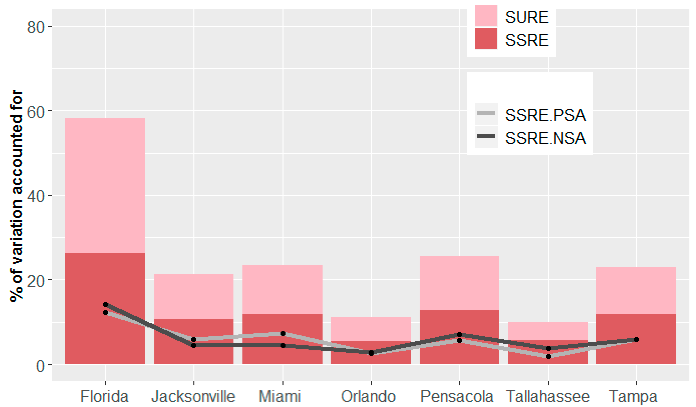
| Models | Florida | Pensacola MSA | Tallahassee MSA | Jacksonville MSA | Orlando MSA | Miami MSA | Tampa MSA |
|---|---|---|---|---|---|---|---|
| RE models intercept-only | 58.39% | 27.13% | 11.64% | 25.14% | 13.68% | 24.46% | 23.88% |
| RE models with covariates | 58.19% | 25.53% | 9.91% | 21.20% | 11.14% | 23.47% | 22.98% |
© 2018 by the authors. Licensee MDPI, Basel, Switzerland. This article is an open access article distributed under the terms and conditions of the Creative Commons Attribution (CC BY) license (http://creativecommons.org/licenses/by/4.0/).
Share and Cite
Hu, L.; Griffith, D.A.; Chun, Y. Space-Time Statistical Insights about Geographic Variation in Lung Cancer Incidence Rates: Florida, USA, 2000–2011. Int. J. Environ. Res. Public Health 2018, 15, 2406. https://doi.org/10.3390/ijerph15112406
Hu L, Griffith DA, Chun Y. Space-Time Statistical Insights about Geographic Variation in Lung Cancer Incidence Rates: Florida, USA, 2000–2011. International Journal of Environmental Research and Public Health. 2018; 15(11):2406. https://doi.org/10.3390/ijerph15112406
Chicago/Turabian StyleHu, Lan, Daniel A. Griffith, and Yongwan Chun. 2018. "Space-Time Statistical Insights about Geographic Variation in Lung Cancer Incidence Rates: Florida, USA, 2000–2011" International Journal of Environmental Research and Public Health 15, no. 11: 2406. https://doi.org/10.3390/ijerph15112406