A Bayesian Approach to Real-Time Monitoring and Forecasting of Chinese Foodborne Diseases

Abstract

Foodborne diseases have a big impact on public health and are often underreported. This is because a lot of patients delay treatment when they suffer from foodborne diseases. In Hunan Province (China), a total of 21,226 confirmed foodborne disease cases were reported from 1 March 2015 to 28 February 2016 by the Foodborne Surveillance Database (FSD) of the China National Centre for Food Safety Risk Assessment (CFSA). The purpose of this study was to make use of the daily number of visiting patients to forecast the daily true number of patients. Our main contribution is that we take the reporting delays into consideration and apply a Bayesian hierarchical model for this forecast problem. The data shows that there were 21,226 confirmed cases reported among 21,866 visiting patients, a proportion as high as 97%. Given this observation, the Bayesian hierarchical model was established to predict the daily true number of patients using the number of visiting patients. We propose several scoring rules to assess the performance of different nowcasting procedures. We conclude that Bayesian nowcasting with consideration of right truncation of the reporting delays has a good performance for short-term forecasting, and could effectively predict the epidemic trends of foodborne diseases. Meanwhile, this approach could provide a methodological basis for future foodborne disease monitoring and control strategies, which are crucial for public health.

1. Introduction

Patients with foodborne diseases often have a lack of awareness about the severity, which may cause them to delay seeing a doctor. Such kinds of delay may easily cover up the outbreak of food safety incidents, which is not conducive to the timely control of the disease outbreaks. Taking the occurred but not yet reported events into account, and tracking the true number of daily cases are essential to rapidly and accurately evaluate current epidemic trends. This stimulated us to study foodborne surveillance data to provide up-to-date information on the growth of the epidemic and current trends, so that from the local health department agency to the national public health agency or institute (e.g., the Center for Disease Control and Prevention in the USA, European Food Safety Agency, the European Centre for Disease Prevention and Control, etc.) can judge whether an outbreak is ongoing, assess the impact of control measures and implement capacity planning.

Previous studies on foodborne disease events have mainly focused on analyzing public surveillance data, estimating the actual incidence of foodborne disease in a country [1,2,3,4,5], and evaluating the burden of disease caused by various types of pathogens [6,7,8,9,10]. Heino et al. [11] proposed a randomized framework to identify the increasing number of foodborne disease events; Neill et al. [12] and Xiao [13,14] applied spatial statistical methods to explore the spatial aggregation of foodborne diseases. When diseases broke out in a certain area, the number of reported cases would surge correspondingly compared to the baseline data, which could be detected by anomaly pattern algorithms through numerical changes [15,16]. Guo et al. [17] designed a detection model of foodborne disease events and risk assessment by integrating the big-data of population, traffic, food production and sales and social media data under a spatio-temporal framework. The above studies ignore the reporting delay factor. However, the additional delays between onset date and reporting date in the public health surveillance database should not be ignored when processing tracking procedures. Lawless [18] firstly estimated the number of events that had occurred but not yet been reported and developed an approach to conduct robust predictions when incorporating random effects based on lately reporting data. Later, a robust algorithm to perform tracking procedures called “nowcasts” was used to correct for reporting delays [19]. Based on such concept, Höhle and an der Heiden [20] proposed a Bayesian nowcasting algorithm to deal with the short-term forecasting of the daily number of reported cases. Salmon et al. [21] improved the outbreak detection algorithms by taking reporting delays into account. Considering that the number of cases can increase dramatically in a matter of days in emerging food safety incidents, in this paper, we focus on how to make use of the daily number of visiting patients to forecast the daily true number of the patients, and we present how the proposed Bayesian nowcasting model could provide a more precise information of epidemic trends.

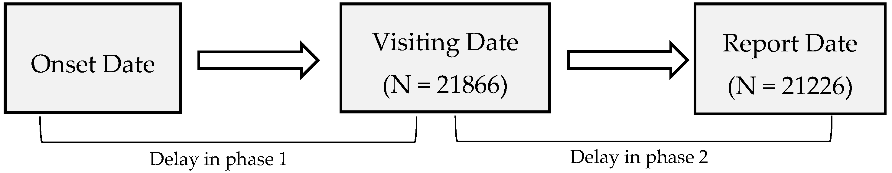
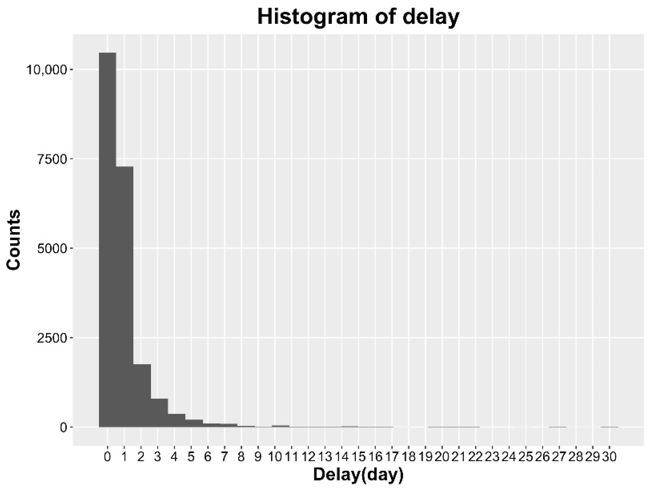
2. Data Material for Foodborne Diseases

Our data, collected from the Foodborne Surveillance Database (FSD) of the China National Centre for Food Safety Risk Assessment (CFSA, Beijing, China), covered confirmed cases in all cities in Hunan Province, China, spanning a year from 1 March 2015 to 28 February 2016.

Table 1. Example of the information collected for the Data set.

Patient ID	Hospital Information			Onset Date	Visit Date	Confirmed
	Province	City	Sentinel Hospital
HN073408-2015-00040	Hunan	Changsha	The Fourth Hospital of Changsha	10 September 2015	11 September 2015	Yes
HN073402-2015-00086	Hunan	Hengyang	Hengyang Centre Hospital of Hunan	7 June 2015	10 June 2015	Yes
HN073002-2015-00128	Hunan	Yueyang	Yueyang Second People’s Hospital	30 September 2015	30 September 2015	Yes

shows examples of our collected data information. Each confirmed case consists of symptom onset date (the self-reported date when the patient was attacked by a foodborne disease), and the visit date (when the patients went to see a doctor). The reporting delay is divided into two phases (Figure 1): Phase 1 is the delay between the onset date and visiting date; phase 2 is the delay between visiting date and the reporting date. In our data set, there are 21,866 patient visits and 21,226 reported confirmed cases.

Generally, the monitoring at the CFSA can be performed on time series aggregated by the date of symptom onset and the date of report arrival at the surveillance database. Specifically, till one day, we define “reported cases” as the currently available counts of patients confirmed by a doctor; and define “occurred cases” as the real number of patients attacked. The goal of nowcasting is to predict the true number of counts from the currently available counts.

Figure 2 plots the trend of foodborne disease, where the blue lines indicate the daily number of “occurred cases” and the red lines indicate the trend line. The curve of “occurred cases” starts to get into a high growth phase from May, and continues to peak till the beginning of November. From the end of November, the number of cases begins to decrease. Figure 3 shows the daily counts of “reported cases” (blue bar) and “occurred cases” (red bar); on 20 July 2015, 371 reported cases of 430 occurred cases (i.e., 86.3%, from 16 July to 20 July) have information available due to the reporting delay. As more reported data comes in, the number of reported cases (blue bar) is getting closer to the number of occurred cases (red bar) in Figure 3.

Figure 4 shows the histogram of observed frequency of delay on the basis of all cases, from which we see that many patients go to see a doctor on the first day when they have foodborne disease, more people have a few days’ delay and seldom have delays of more than one week. To facilitate understanding, we assume the maximum delay occurs up to 5 days due to the $3\sigma$ principle getting from the information in Figure 4. Note that the data will become less reliable and the information contained is not accurate when the delay becomes very large. We denote $p_d,d=0,1,\dots ,5$, as the observed proportion of the number of patients with delay $d$ days to the total number of patients given a time span. Note that $p_5$ includes delay with days larger than or equal to 5 days, and ${\sum }_{d=0}^5{p}_d=1$.

From a seasonal perspective of delay distribution, Figure 5 suggests that the distribution of reporting delay does not change significantly with time, which therefore motivates us to assume that the patient behavior (corresponding to delay distribution) in a given region is stable with four seasons, if nothing else intervenes (e.g., policy).

3. Bayesian Nowcasting

Nowcasting is defined as the prediction of the present—the very near future or the very recent past. Recently, it has been regarded as a useful tool to real-time monitor the disease surveillance data [19,20], personal pro-health outdoor activities [22], and forecast the epidemics in public health settings [23]. In this paper, we apply a Bayesian nowcasting model proposed by Höhle and an der Heiden [20] to forecast the daily total number of cases. Thanks to Salmon et al. [24] who provided a convenient R package “surveillance” and the inference for the model could be easily implemented. The R package surveillance also contains a few other nowcasting methods which we also tried and did comparisons with using the scoring rules implemented in the package. The results are shown in Section 4. Below we review the model.

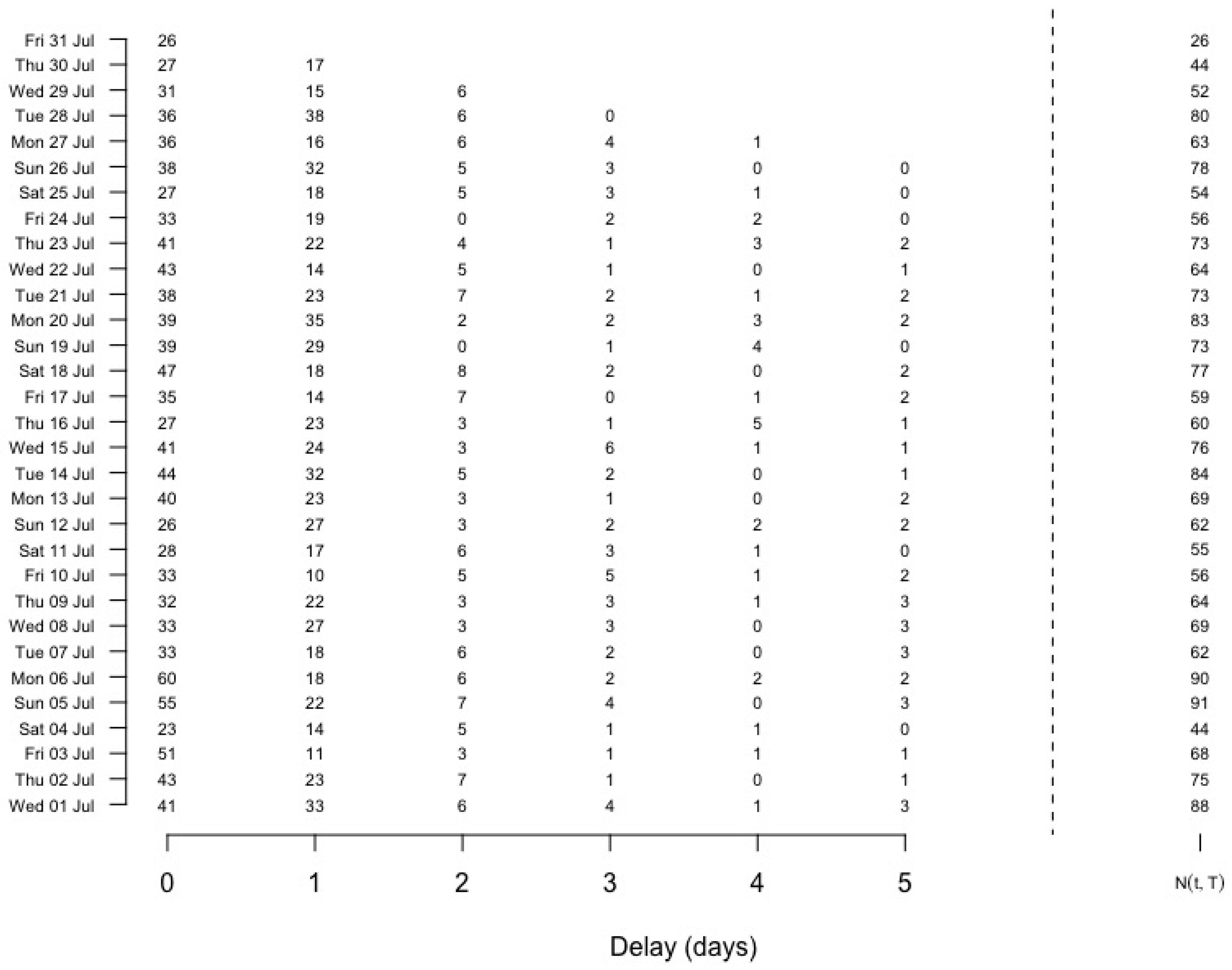
3.1. Notation and Assumptions

We place our study in a discrete time setting where each unit represents a day. We use the notation of Lawless [18] to describe the prediction of the currently actual number of patients in the presence of delay. Let $n_{t,d}$ be the number of patients with foodborne disease at time $t$ but reported with a delay of $d$ days, which means that, these $n_{t,d}$ patients get foodborne disease at time $t$, but they arrive on hospital at time $t+d$. $t$ takes values on $\left\{0,\cdots ,T\right\}$, $T$ denotes the current day or “now”, and $d$ takes values on $\left\{0,\cdots ,\mathrm{D}\right\}$. Typically, one can assume that the maximum delay occurs up to $D$ days since the data will become less reliable and the information contained is not accurate when the delay time $d$ becomes very large. In our study, reports with a delay larger than $D$ are included in the category of delay being “D days”. Note that when $d>T-t$, we could not know $n_{t,d}$, because at time $T$, the patients have not gone to hospital yet. So our data is right-truncated type of data. Formally, we devote $N_{t,T}\triangleq N\left(t,T\right)={\sum }_{d=0}^{\min \left(T-t,D\right)}{n}_{t,d}$ to be observed cases reported (those who go to hospital already) until time $T$. Thus with the limit of maximal delay, the real number of cases occurred at time $t$, $0\le t\le T$, is:

$$N_t\triangleq {\displaystyle \sum _{d=0}^D}{n}_{t,d}=\{\begin{array}{c}{\displaystyle \sum _{d=0}^D}{n}_{t,d},T-t\ge D,\mathrm{e}.\mathrm{g}.,\mathrm{full}\mathrm{data}\\ {\displaystyle \sum _{d=0}^{T-t}}{n}_{t,d}+{\displaystyle \sum _{d=T-t+1}^D}{n}_{t,d},T-t<D,\mathrm{e}.\mathrm{g}.,\mathrm{truncated}\mathrm{data}\end{array}$$

Note that $N_t$ is right-truncated for $t$ larger than $T-D$. Our goal is to estimate the unobserved right-truncated $N_t$. We use Figure 6 to visualize the data structure. Each row indicates the total number of cases occurred at time t, the shaded box $N_t-N_{t,T}$ represents the cases that occurred but not yet reported. In order to facilitate model description, we divided the solution space into three parts: $A_t=\left\{\left(t,d\right):0\le t\le T,0\le d\le D\right\}$ covers all observed data and unobserved data while $O_t=\left\{\left(t,d\right):0\le t\le T,0\le d\le \min \left(T-t,D\right)\right\}$ contains observed $n_{O_t}$ only and $U_t=A_t\backslash O_t$ contains unobserved $n_{U_t}$ only. We draw them as the light gray trapezoid and as the darker gray triangle in Figure 6 respectively.

3.2. Predict the Distribution for $N_t$

For the convenience of the reader, we describe the inference approach stated in Section 3.2 of Höhle and an der Heiden in [20] in some greater detail.

Define $p_d$ as the (time-homogeneous) probability that a case will have a reporting delay of $d$ days. The $p_d$’s satisfy the following equation: ${\sum }_{d=0}^D{p}_d=1$. Following Kalbfleisch and Lawless’s [25] and Zeger et al.’s [26], we assume that the occurrence time of cases follows an underlying inhomogeneous Poisson process. A reasonable data generating process for the daily number of cases is thus as follows:

$$\begin{array}{cc}\hfill N_t|{\lambda }_t& \sim \mathrm{Po}\left({\lambda }_t\right)\hfill \\ \hfill \left(n_{t,D},n_{t,D-1},\cdots ,n_{t,0}\right)’|N_t,\mathbf{p}& \sim \mathrm{MN}\left(N_t,{\left(p_D,p_{D-1},\cdots ,p_0\right)}^{\prime }\right)\hfill \end{array}$$

(1)

where $\mathrm{Po}\left(\lambda \right)$ denotes the Poisson distribution with expectation $\lambda >0$ and $\mathrm{MN}\left(N,\mathbf{p}\right)$ denotes the multinomial distribution with size parameter $N$ and probability vector $\mathbf{p}$. Nowcasting for a given time $T$ can thus be divided into steps of determining the ${\lambda }_t$’s, estimating the unknown delay distribution (i.e., the $p_d$’s) and finally predicting the unobserved $n_{t,d}$’s in order to compute the total $N_t$. As $T$ increases, and if the assumption about a time-homogeneous delay distribution is acceptable, the available data make it possible to estimate the delay distribution better and better and, hence, the quality of the predictions near $T$ improves with time.

Consider a fixed time $T$ and define ${\mathbf{p}}_T=\left(p_{T,D},p_{T,D-1},\cdots ,p_{T,1}\right)$’ as the probability vector denoting that a case is reported with a delay of $d$ days given the observed incomplete information at time $T$, i.e., the set of $n_{t,d},$ where $t+d\le T$. We choose as prior distribution the generalised Dirichlet distribution $GD\left(\mathsf{\alpha },\mathsf{\beta }\right)$ with fixed constants $\mathsf{\alpha }={\left({\alpha }_0,{\alpha }_1,\cdots ,{\alpha }_D\right)}^{\prime }$ and $\mathsf{\beta }={\left({\beta }_0,{\beta }_1,\cdots ,{\beta }_D\right)}^{\prime }$. Now we use Property 3 in the Web appendix of [20] that shows that the posterior of $\mathbf{p}$ under right-truncated multinomial sampling is again a GD distribution with parameters ${\mathsf{\alpha }}_T^{\ast },{\mathsf{\beta }}_T^{\ast }$ given by

$$\begin{array}{cc}\hfill {\alpha }_{T,i}^{\ast }& ={\alpha }_i+{\displaystyle \sum _{\tau =0}^{T-D+i}}{n}_{\tau ,D-i}\hfill \\ \hfill {\beta }_{T,i}^{\ast }& ={\beta }_i+{\displaystyle \sum _{\tau =0}^{T-D+i}}(N_{\tau ,\tau +D-i}-n_{\tau ,D-i}),i\in \left\{0,\cdots ,D-1\right\}.\hfill \end{array}$$

(2)

Hence, for a given $T$ we can assume the following model hierarchy for the time points $t\in \left\{T-D,\cdots ,T\right\}$:

$$\begin{array}{cc}\hfill {\mathbf{p}}_T& \sim GD\left({\mathsf{\alpha }}_T^{\ast },{\mathsf{\beta }}_T^{\ast }\right)\hfill \\ \hfill {\lambda }_t& \sim Ga\left(a_{\lambda },b_{\lambda }\right)\hfill \\ \hfill N_t|{\lambda }_t& \sim Po\left({\lambda }_t\right)\hfill \\ \hfill N_{t,T}|N_t,{\mathbf{p}}_T& \sim \mathrm{Bin}\left(N_t,q_{T,T-t}\right),\hfill \end{array}$$

(3)

where $q_{T,d}={\displaystyle \sum _{\delta =0}^d}{p}_{T,\delta }$ is the proportion reported within a delay of $d$ days. We denote by $Ga\left(a_{\lambda },b_{\lambda }\right)$ the Gamma distribution with parameters $a_{\lambda }>0,b_{\lambda }>0$. For this hierarchical model, the marginal distribution of $N_t$ is a negative binomial distribution with the following mean and variance:

$$\begin{array}{cc}\hfill E\left(N_t\right)& ={\mu }_{\lambda }=a_{\lambda }{b}_{\lambda }\hfill \\ \hfill \mathrm{Var}\left(N_t\right)& ={\mu }_{\lambda }+\frac{{\mu }_{\lambda }^2}{a_{\lambda }}.\hfill \end{array}$$

(4)

To estimate $N_t$ given the observed counts $n_{t,d}$ at time $T$, we have to perform two steps: (1) update the delay distribution ${\mathbf{q}}_T$ and (2) update the prediction for $N_t$:

• For the given T we compute ${\alpha }_T^{\ast },{\beta }_T^{\ast }$ as stated above. We then We draw for $k=1,\dots ,K$ random vectors ${\mathbf{p}}_T^{\left(k\right)}\sim GD\left({\mathsf{\alpha }}_T^{\ast },{\mathsf{\beta }}_T^{\ast }\right)$ by the algorithm of Wong (1998) and calculate

  $$q_{T,d}^{\left(k\right)}={\displaystyle \sum _{\delta =0}^d}{p}_{T,\delta }^{\left(k\right)}.$$

  (5)
• Given the updated delay distribution ${\mathbf{q}}_T^{\left(k\right)}$ and the observed counts $n_{t,d}$, we can now update the prediction of $N_t,t=T-D,\cdots ,T$.

For $n\in \left\{0,1,2,\cdots \right\}$ we approximate by Monte Carlo sampling

$$f(N_t=n|N_{t,T})\approx \frac{1}{K}{\displaystyle \sum _{k=1}^K}{f}_{n,t}^{\left(k\right)},t\in \left\{T-D,\cdots ,T\right\}$$

(6)

An application of Bayes theorem provides $f_{n,t}^{\left(k\right)}={\tilde{f}}_{n,t}^{\left(k\right)}/c_t^{\left(k\right)}$, where $c_t^{\left(k\right)}={\sum }_{n=0}^{\infty }{\tilde{f}}_{n,t}^{\left(k\right)}$ is the normalization constant and

$${\tilde{f}}_{n,t}^{\left(k\right)}=f(N_{t,T}|N_t=n,q_{T,T-t}^{\left(k\right)})f(N_t=n|{\lambda }_t)f\left({\lambda }_t\right)$$

(7)

for all $t\in \left\{T-D,\cdots ,T\right\}$. The factors of the last equation can be evaluated using the distributional assumptions of the model hierarchy. For numerical convenience we do not sum over the entire support $\left\{0,1,2,\cdots \right\}$ to get the normalization, but instead approximate

$$c_t^{\left(k\right)}\approx {\displaystyle \sum _{n=0}^{N_{\max }}}{\tilde{f}}_{n,t}^{\left(k\right)},$$

(8)

where $N_{\max }$ is chosen sufficiently large.

4. Main Results

4.1. Setup for Hyper-Parameters

We applied the Bayesian hierarchical model described above to the foodborne surveillance data time series of Hunan Province in China. To decide the hyper-parameter $\mathbf{\alpha },\mathbf{\beta }$ in the prior of $\mathit{p}$ and $a_{\lambda },b_{\lambda }$ in the prior of ${\lambda }_t$, we use the empirical Bayes ideas. Analyzing the observed data from 1 March 2015 to 28 February 2016, we found that the mean and variance of $N_t$ from the dataset are 57 and 982 respectively. Thus solving the following equations, we get the values for hyperparameters $a_{\lambda },b_{\lambda }$:

$$57\approx E\left(N_t\right)={\mu }_{\lambda }=a_{\lambda }{b}_{\lambda },$$

$$982\approx Var\left(N_t\right)={\mu }_{\lambda }+\frac{{\mu }_{\lambda }^2}{a_{\lambda }}$$

By the delay distribution shown in Figure 4, we take the maximum delay $D=5$ days. Retrospectively, we can transform the historical available data into a final reporting triangle, which clearly shows the delay information. For example, in Figure 7, each cell $n_{t,d}$ indicates a count number that occurred at a given time point $t$ but reported with a delay of $d$ while the sum over all counts in a row is the corresponding $N_{t,T}$ for each day $t$ shown on the right bars, where $T=$ “31 July 2015”. Also we can work out the cumulative frequency for each delay based on the whole dataset, which provides informative prior for $\mathit{p}$.

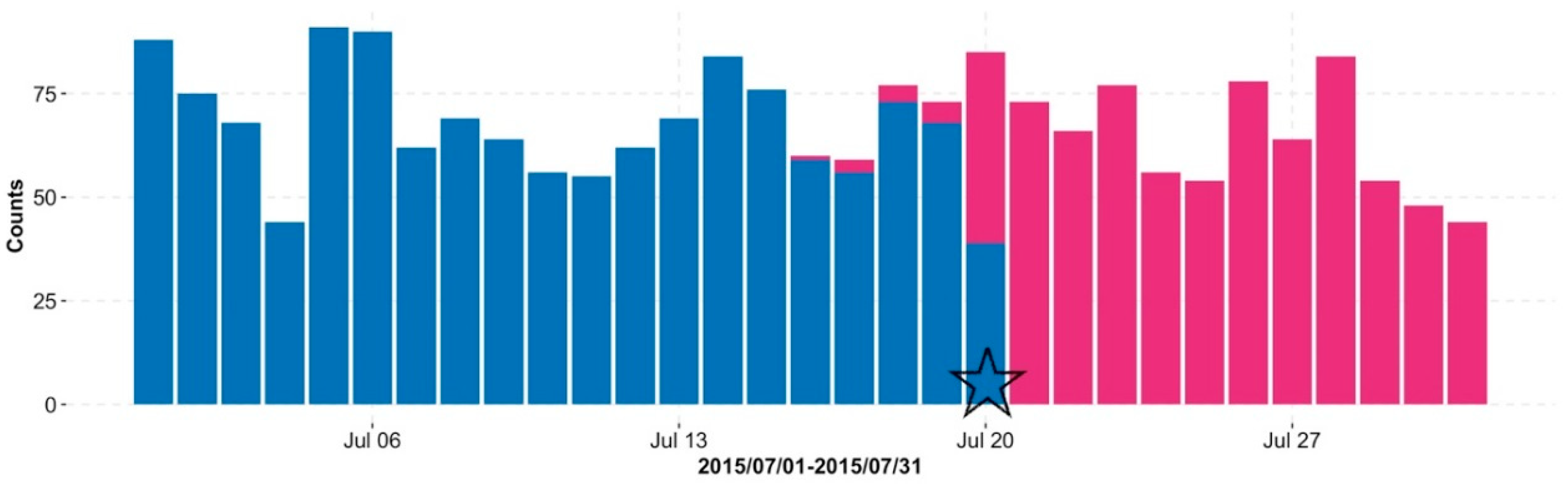
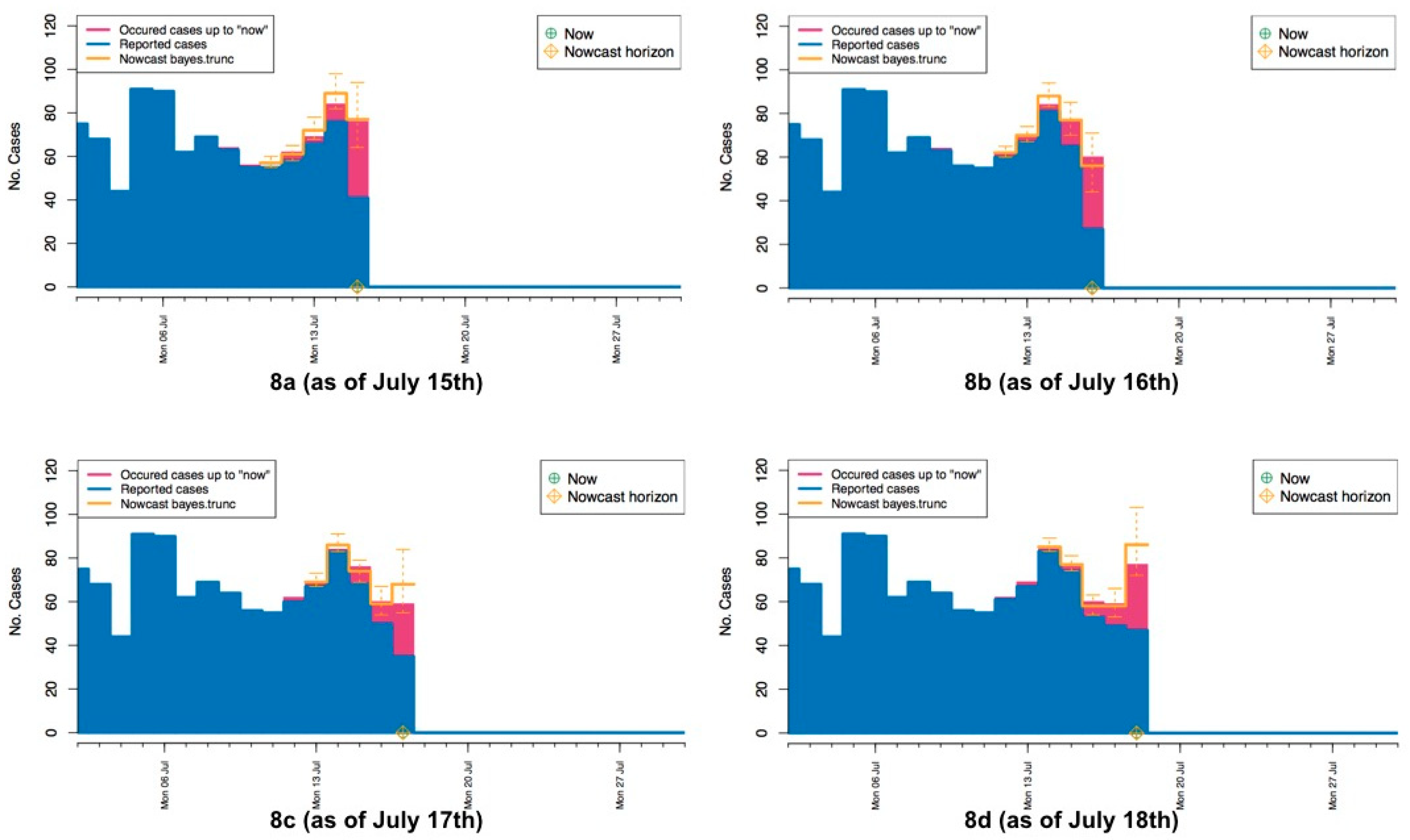
4.2. Daily Surveillance

Below we apply the described BNT approach to the data set of foodborne patients described above. Here we set a time span 5 days to do the nowcasting. For each current day T, we try to predict the unobserved occurred cases $N_t$’s for $t\in \left\{T-4,T-3,T-2,T-1,T\right\}$. We give an animation of the details of our nowcasting process in the Supplementary Materials File S1. To explain the animation, we show four pictures for the continuous four days from 15 to 18 July in Figure 8. These pictures give the nowcasting process for predicting the numbers $N_t$’s of cases really occurred to the current days in July. Figure 8a takes 15 July as the current day, the numbers of reported cases until 15 July are drawn in blue, and the numbers of real occurred cases are drawn in red. Since there are 5 days for occurred cases to be reported, the accurate numbers of occurred cases for the current 5 days from 11 to 15 July may not be available as of 15 July. The goal is to predict the numbers of occurred cases for these current 5 days. In Figure 8a, the prediction of these numbers are drawn in yellow, the bold yellow bar indicates the median of the prediction distribution of occurred cases, the two short yellow bars indicate the 2.5% and 97.5% quantiles of the prediction distribution. The predicted number of occurred cases for 15 July is very close to the real number, although the interval between two bounds of the prediction distribution for 15 July is longer. The predicted number for 14 July is a little higher than the real number, although the interval is much shorter than that for 15 July. Similarly, Figure 8b–d show the predictions on 16–18 July, respectively, and it can be seen that interval for 15 July becomes shorter and shorter. From the four pictures drawn from the animation given in the Supplementary Materials File S1, we can see the predicted numbers are quite close to the real numbers of occurred cases for these four days, and the intervals all cover the real numbers of occurred cases.

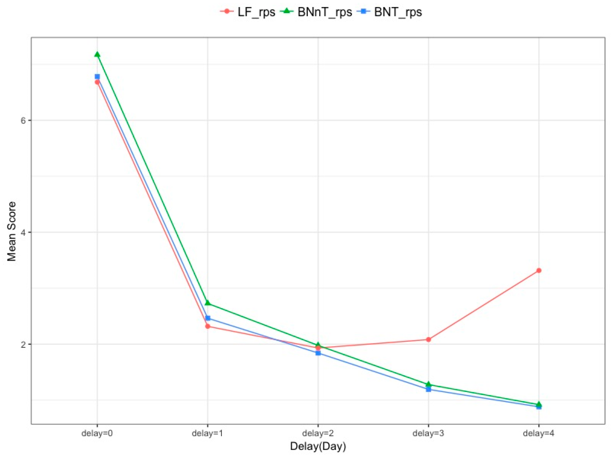
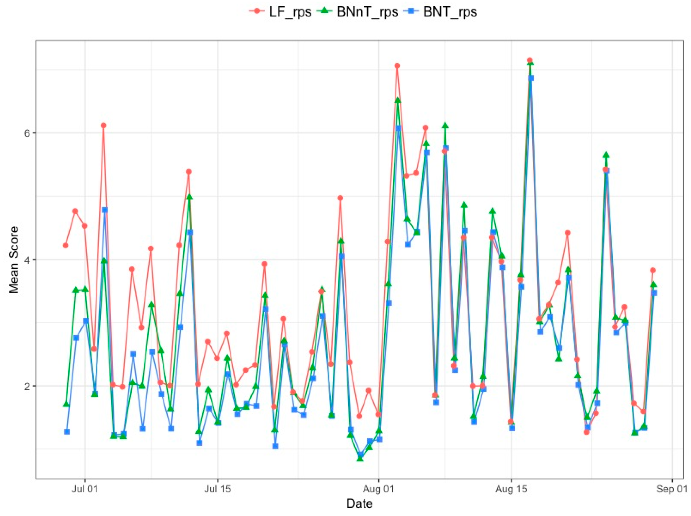
4.3. Evaluating the Nowcasting

In this section, three different nowcasting procedures will be compared: the Lawless [18] frequency (LF) method with the consideration of the right-truncated nature and two Bayesian procedures, one is BNT method described in this paper and Bayesian nowcasting with no truncation (BNnT) method by Höhle and an der Heiden [20] ignoring the right truncation.

Before doing comparisons, we predict the numbers of occurred cases for 5 days on each current day T. We take T from 30 June 2015 to 30 August 2015, totally 63 days and so 5 × 63 = 315 nowcastings will be calculated. Considering a specific time T (for example “now”) we predict $N_t$’s for $t\in \left\{T-4,T-3,T-2,T-1,T\right\}$. To evaluate the performance of different nowcasting approaches, we use three scoring rules:

(i)

Logarithmic score (logS) [27]:

$$logS\left(P_t^T,N_t\right)=-\log \left(f_{P_t^T}\left(N_t\right)\right)$$

(ii)

Ranking probability score (RPS) [28,29]:

$$RPS\left(P_t^T,N_t\right)={\displaystyle \sum _k^N}\left(F_t^T\left(N_t\right)-\mathbf{1}\left(N_t\le k\right)\right)$$

where $P_t^T$ is the predictive distribution for time t based on the information available at T and with $N_t$ being the number of occurred cases. $f_{P_t^T}(\cdot )$ is the probability mass function (PMF) of the predictive distribution $P_t^T$, and where $F_{P_t^T}(\cdot )$ denotes the cumulative distribution function (CDF) of the predictive distribution $P_t^T$. And from the data prior information, here we choose $N_{max}=$ 300.

(iii)

The proportion of times that the observed value lay outside the equal-tailed 95% predicted interval (OutCI).

Such rules allow investigating calibration and sharpness of predictive distribution. The higher probability of the forecast distribution for the actual observed value is, the better the prediction is. It means that the lower the score is, the better the performance is.

Table 2. Mean scores for different nowcasting methods.

Method	RPS	logS	OutCI
BNT	2.63	2.52	0.07
BNnT	2.81	2.80	0.12
LF	3.27	2.58	0.07

gives the mean scores obtained by averaging over the 315 nowcastings, which illustrates that BNT method described in this paper has an overall best performance based on these three evaluation rules compared to other existing methods (BNnT method and LF method).

We consider the comparison among LF method, BNT method described in this paper and BNnT method, here we also predict the numbers of occurred cases for 5 days from the current day 0 to 4 days ago. Figure 9 shows the mean scores of RPS obtained by averaging for $t\in \left\{T-4,T-3,T-2,T-1,T\right\}$ from 315 nowcastings. The mean scores are the largest for $\mathrm{delay}=0$ among all delays. When the delay increases, more information is collected, and the LF method (red line) and BNT method (blue line) have a better performance with $\mathrm{delay}\le 2$. When $\mathrm{delay}\ge 2$ days, the BNT method appears to perform best.

Finally, we compare the mean scores of RPS among LF method, BNT method described in this paper and BNnT method with considering the time span from 1 July to 30 August. Figure 10 shows that BNT method (blue line) outperforms the LF method (red line) and BNnT method (green line).

5. Discussion

In this paper, we introduced a Bayesian hierarchal approach to monitor and forecast in real-time Chinese foodborne disease outbreaks based on the public health surveillance data if reporting delays are present. Such delay-adjusting tracking procedures can provide daily information on the epidemic trends by predicting the daily true number of patients.

In fact, the delay could be divided into two phases. Phase 1 is the delay from the onset to the doctor visit, and this is the delay of the patients in seeking medical treatments. Since the foodborne disease is not a serious disease requiring immediate emergency, many patients are not in a hurry to go to the hospital for treatment, which may cover up the outbreak of a food safety incident. Phase 2 is the delay between the visit date and the hospital reporting date. The delay distribution in this stage is very complicated. Due to the difference for medical level of each hospital, the efficiency of the experiment, the doctor’s understanding of the foodborne disease and the definition of the cases, etc., the diagnosis report will be delayed. This is the delay in phase 2. References [19,20,21] used the number of patients reported in the hospital to predict the number of occurred cases. The cycle is very long from the onset to the diagnosis reported, which couldn’t predict the number of cases, or grasp the trends of the disease in a timely way. Therefore, in view of this, our model has the following advantages: First, when the data is complete and there is hospital-confirmed report data in hand, our model uses the number of confirmed patients to predict the number of occurred cases, a procedure similar to that of [20,21]. Then, if the data is incomplete, for example, we only have the visiting data till today, we could use the number of visiting patients to predict the occurred cases, which may lead to a very small overestimation of the number of occurred cases, but least not underestimate them. However, it makes the prediction ahead of days (the delay in Phase 2). In fact, our collected data shows that there are 21,226 confirmed cases among 21,866 visiting patients, a proportion as high as 97%. Early warning of disease outbreaks could avoid long delays from patient visit to disease confirmation, which can greatly shorten the forecast period, detecting possible food safety incidents in a more timely fashion. It is very significant in this regard.

As future work, since the number of visits is used to predict the number of occurred cases that will be overestimated (at least not underestimated), we will use the empirical data to obtain the proportion of confirmed cases among the visiting patients. Under this condition, the information of the proportion can be used to predict the number of occurred cases. We will also consider applying a compound Poisson model to solve the problem of overestimation of the number of occurred cases. Meanwhile, other covariates including city, age, occupation, etc., will also be considered. How to analyze and model the foodborne disease surveillance data, and how to detect the outbreak based on historical data, even the casual inference to pathogenic factors, are all issues to be studied in the future.

References

1. Mead, P.S.; Slutsker, L.; Dietz, V.; Mccaig, L.F.; Bresee, J.S.; Shapiro, C.; Griffin, P.M.; Tauxe, R.V. Food-related illness and death in the United States. Emerg. Infect. Dis. 1999, 5, 607–625. [Google Scholar] [CrossRef]
2. Astride, K.H.; McPherson, M.; Kirk, M.D.; Knope, K.; Gregory, J.; Kardamanidis, K.; Bell, R. Foodborne disease outbreaks in Australia 2001–2009. Food Aust. 2011, 63, 44–50. [Google Scholar]
3. Gould, L.H.; Mungai, E.A.; Johnson, S.D.; Richardson, L.T.C.; Williams, I.T.; Griffin, P.M. Surveillance for foodborne disease outbreaks—United States, 2009–2010. Morb. Mortal. Wkly. Rep. 2013, 60, 1197–1202. [Google Scholar]
4. Masoumi, A.H.; Gouya, M.M.; Soltandallal, M.M.; Aghili, N. Surveillance for foodborne disease outbreak in Iran, 2006–2011. Med. J. Islam. Repub. Iran 2015, 29, 285. [Google Scholar]
5. Yong, S.K.; Lee, S.H.; Joo, Y.; Bahk, G.J. Inverstigation of the experience of foodborne illness and estimation of the incidence of foodborne disease in south Korea. Food Control 2015, 47, 226–230. [Google Scholar]
6. World Health Organization. WHO Estimates of the Global Burden of Foodborne: Foodborne Diseases Burden Epidemiology Reference Group 2007–2015; WHO Press: Geneva, Switzerland, 2015; ISBN 978-9-24-156516-5. [Google Scholar]
7. Voetsch, A.C.; Van Gilder, T.J.; Angulo, F.J.; Farley, M.M.; Shallow, S.; Marcus, R.; Cieslak, P.R.; Deneen, V.C.; Tauxe, R.V. Emerging Infections Program FoodNet Working Group. FoodNet estimate of the burden of illness caused by nontyphoidal Salmonella infections in the United States. Clin. Infect. Dis. 2004, 38, S127–S134. [Google Scholar] [CrossRef] [PubMed]
8. Flint, J.A.; Van Duynhoven, Y.T.; Angulo, F.J.; Delong, S.M.; Braun, P.; Kirk, M.; Scallan, E.; Fitzgerald, M.; Adak, G.K.; Sockett, P. Estimating the Burden of Acute Gastroenteritis, Foodborne Disease, and Pathogens Commonly Transmitted by Food: An International Review. Clin. Infect. Dis. 2005, 41, 698–704. [Google Scholar] [CrossRef] [Green Version]
9. Scallan, E.; Hoekstra, R.M.; Widdowson, M.; Hall, A.; Griffin, P. Foodborne illness acquired in the United States. Emerg. Infect. Dis. 2011, 17, 1339–1340. [Google Scholar] [CrossRef]
10. Bouwknegt, M.; Pelt, W.V.; Havelaar, A.H. Scoping the Impact of Changes in Population Age-Structure on the Future Burden of Foodborne Disease in The Netherlands, 2020–2060. Int. J. Environ. Res. Public Health 2013, 10, 2888–2896. [Google Scholar] [CrossRef] [PubMed] [Green Version]
11. Heino, J.; Toivonen, H. Automated Detection of Epidemics from the Usage Logs of a Physicians Reference Database. In Proceedings of the European Conference on Principles of Data Mining and Knowledge Discovery, Cavtat-Dubrovnik, Croatia, 22–26 September 2003; Volume 2838, pp. 180–191. [Google Scholar]
12. Neill, D.B.; Moore, A.W. A Fast Multi-Resolution Method for Detection of Significant Spatial Disease Clusters. Adv. Neural Inf. Process. Syst. 2004, 13, 651–658. [Google Scholar]
13. Xiao, H.; Xiao, G.X. Application of space-time permutation scan statistics inbacillary dysentery surveillance. Chin. J. Food Hyg. 2014, 26, 83–87. [Google Scholar]
14. Xiao, G.X.; Xiao, H. Current status and prospect of spatial statistics in food safety. Chin. J. Food Hyg. 2016, 28, 409–414. [Google Scholar]
15. Wong, W.K.; Moore, A.W.; Cooper, G.F.; Wagner, M.M. Bayesian network anomaly pattern detection for disease outbreaks. In Proceedings of the 20th International Conference on Machine Learning (ICML-03), Washington, DC, USA, 21–24 August 2003; pp. 808–815. [Google Scholar]
16. Yang, E.; Park, H.W.; Choi, Y.H.; Kim, J.; Munkhdalai, L.; Musa, I.; Ryu, K.H. A Simulation-Based Study on the Comparison of Statistical and Time Series Forecasting Methods for Early Detection of Infectious Disease Outbreaks. Int. J. Environ. Res. Public Health 2018, 15, 966. [Google Scholar] [CrossRef] [PubMed]
17. Guo, D.H.; Cui, W.J.; Guo, Y.C.; Li, J.H.; Center, S.D. Foodborne disease event detection and risk assessment based on big-data. Syst. Eng. Theory Pract. 2015, 35, 2523–2530. [Google Scholar]
18. Lawless, J.F. Adjustments for reporting delays and the prediction of occurred but not reported events. Can. J. Stat. 1994, 22, 15–31. [Google Scholar] [CrossRef]
19. Donker, T.; Boven, M.V.; Ballegooijen, W.M.V.; Klooster, T.M.V.; Wielders, C.C.; Wallinga, J. Nowcasting pandemic influenza A/H1N1 2009 hospitalizations in the Netherlands. Eur. J. Epidemiol. 2011, 26, 195–201. [Google Scholar] [CrossRef] [PubMed] [Green Version]
20. Höhle, M.; an der Heiden, M. Bayesian nowcasting during the STEC O104:H4 outbreak in Germany, 2011. Biometrics 2014, 70, 993–1002. [Google Scholar] [CrossRef] [Green Version]
21. Salmon, M.; Schumacher, D.; Stark, K.; Hohle, M. Bayesian outbreak detection in the presence of reporting delays. Biom. J. 2015, 57, 1051–1067. [Google Scholar] [CrossRef]
22. Krzyścin, J.W.; Lesiak, A.; Narbutt, J.; Sobolewski, P.; Guzikowski, J. Perspectives of UV nowcasting to monitor personal pro-health outdoor activities. J. Photochem. Photobiol. B 2018, 184, 27–33. [Google Scholar] [CrossRef] [PubMed]
23. Wang, L.; Wu, J.T. Characterizing the dynamics underlying global spread of epidemics. Nat. Commun. 2018, 9, 218. [Google Scholar] [CrossRef]
24. Salmon, M.; Schumacher, D.; Höhle, M. Monitoring count time series in R: Aberration detection in public health surveillance. J. Stat. Softw. 2016, 70, 1–35. [Google Scholar] [CrossRef]
25. Kalbfleisch, J.D.; Lawless, J.F. Inference Based on Retrospective Ascertainment: An Analysis of the Data on Transfusion-Related AIDS. J. Am. Stat. Assoc. 1989, 84, 360–372. [Google Scholar] [CrossRef]
26. Zeger, S.L.; See, L.C.; Diggle, P.J. Statistical methods for monitoring the AIDS epidemic. Stat. Med. 1989, 8, 3–21. [Google Scholar] [CrossRef] [PubMed]
27. Murphy, A.H. A Note on the Ranked Probability Score. J. Appl. Meteorol. 1971, 10, 155. [Google Scholar] [CrossRef]
28. Czado, C.; Gneiting, T.; Held, L. Predictive Model Assessment for Count Data. Biometrics 2009, 65, 1254. [Google Scholar] [CrossRef]
29. Kaufman, J.; Lessler, J.; Edlund, S.; Hu, K.; Douglas, J.; Thoens, C.; Kasbohrer, A.; Filter, M.; Harry, A.; Appel, B. Correction: A likelihood-based approach to identifying contaminated food products using sales data: Performance and challenges. PLoS Comput. Biol. 2014, 10, e1003692. [Google Scholar] [CrossRef] [PubMed]
Figure 1. Illustration of reporting delay phases.
Ijerph 15 01740 g001
Figure 2. Seasonal trend of food-borne diseases during 1 March 2015 and 28 February 2016.
Ijerph 15 01740 g002
Figure 3. Daily number of “occurred cases” (red bar) with foodborne disease in retrospect. The blue bar denotes the number of available” reported cases” as of 20 July 2015 (indicated by the pentagram symbol).
Ijerph 15 01740 g003
Figure 4. Histogram of the observed frequency of delays.
Ijerph 15 01740 g004
Figure 5. Seasonal distribution of delays. Here p d ,   d = 0 , 1 , , 4 , 5 , indicates the observed proportion of delay with d days. Category p 5 includes delay with days larger than or equal to 5 days.
Ijerph 15 01740 g005
Figure 6. Data structure of our data and model. Available observations spanned by n 0 , 0 ,   n T , 0 ,   n T D , D and n 0 , D are in the right-angled trapezoid O T while the triangle U T spanned by n T , 1 ,   n T D + 1 , D and n T , D represents the cases that occurred but not yet reported. Delays greater than D are rare and ignored.
Ijerph 15 01740 g006
Figure 7. Reporting triangle at time 31 July 2015. Delays larger than 5 are covered in category “Delay = 5”.
Ijerph 15 01740 g007
Figure 8. Pictures from animation of the nowcasting procedure (ad) “now” = 15 July 2015–“now” = 18 July 2015. The yellow crosshairs indicate the current day T.
Ijerph 15 01740 g008
Figure 9. The mean scores of RPS comparison by different delays.
Ijerph 15 01740 g009
Figure 10. The Mean score as a function of the time points.
Ijerph 15 01740 g010