Land Use Regression Modelling of Outdoor NO2 and PM2.5 Concentrations in Three Low Income Areas in the Western Cape Province, South Africa


 , , , , ,
Abstract
:1. Introduction
2. Materials and Methods
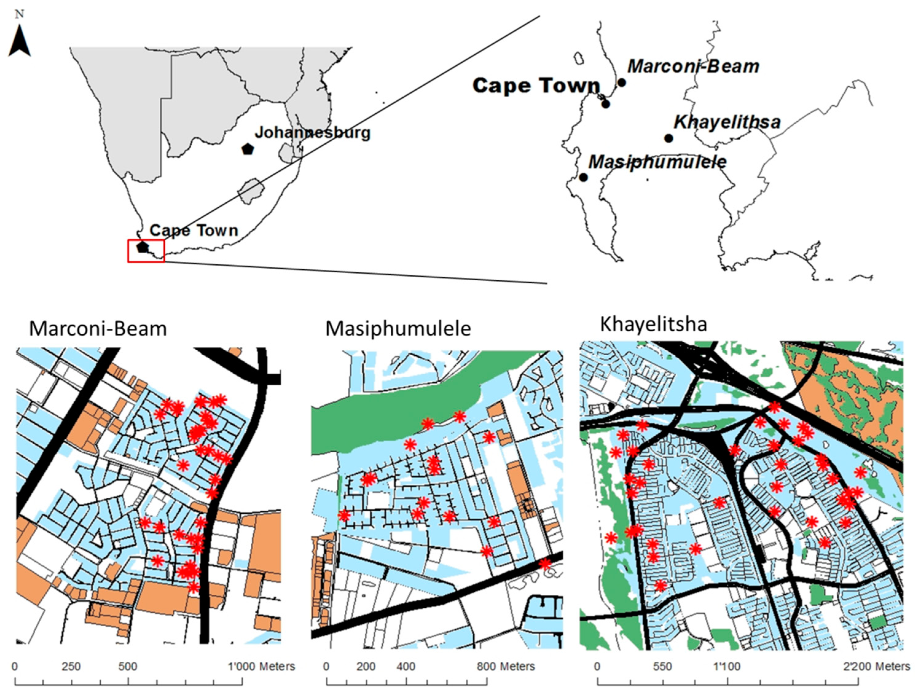
2.1. Study Area
2.2. Measurements
2.3. Geographical Predictor Data and Local Sources
2.4. Temporal Adjustment
2.5. LUR Modelling
2.6. Validation
3. Results
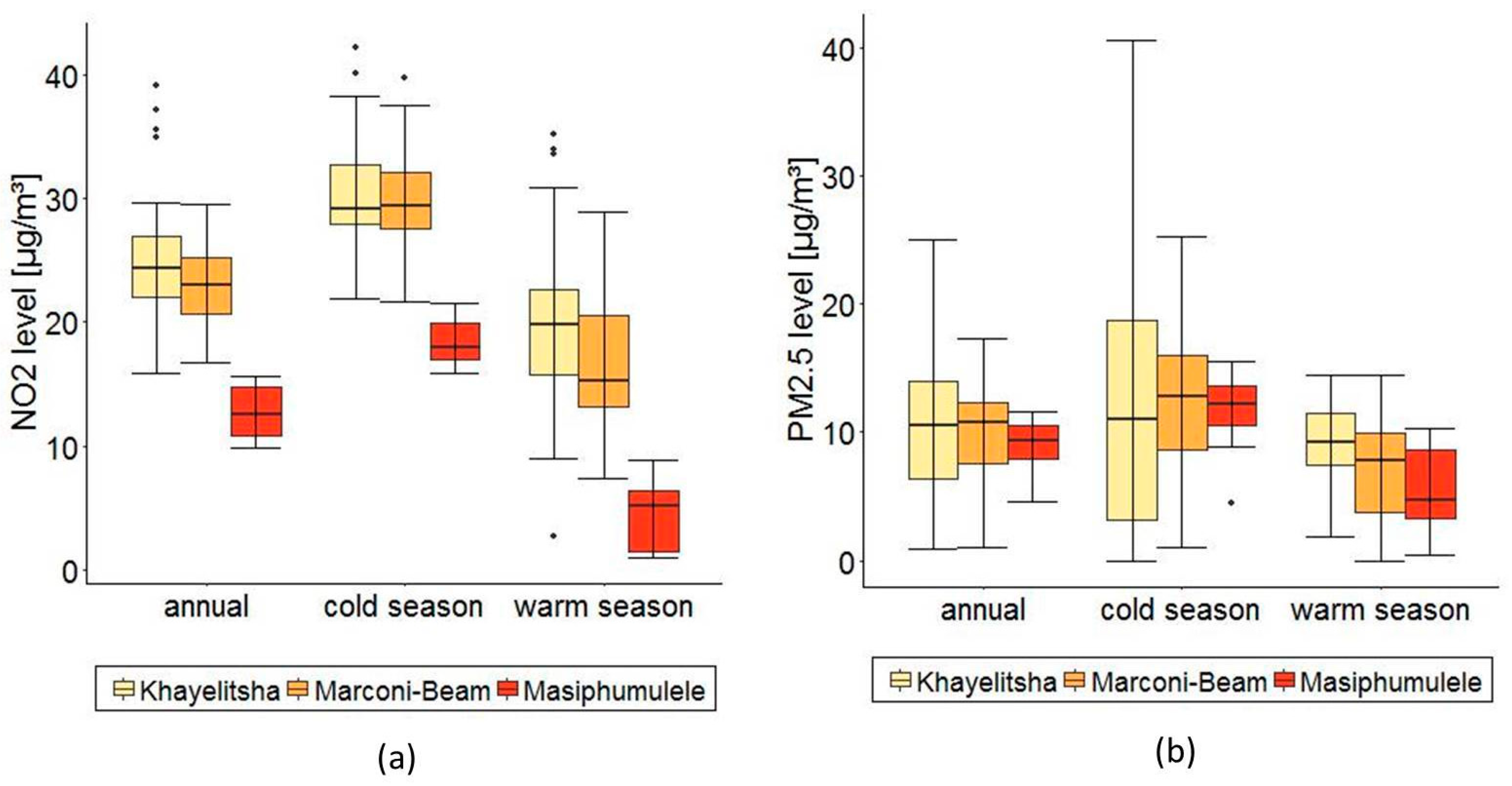
3.1. Measurements
3.2. Temporal Adjusted NO2 and PM2.5 Values
3.3. NO2 and PM2.5 LUR Models
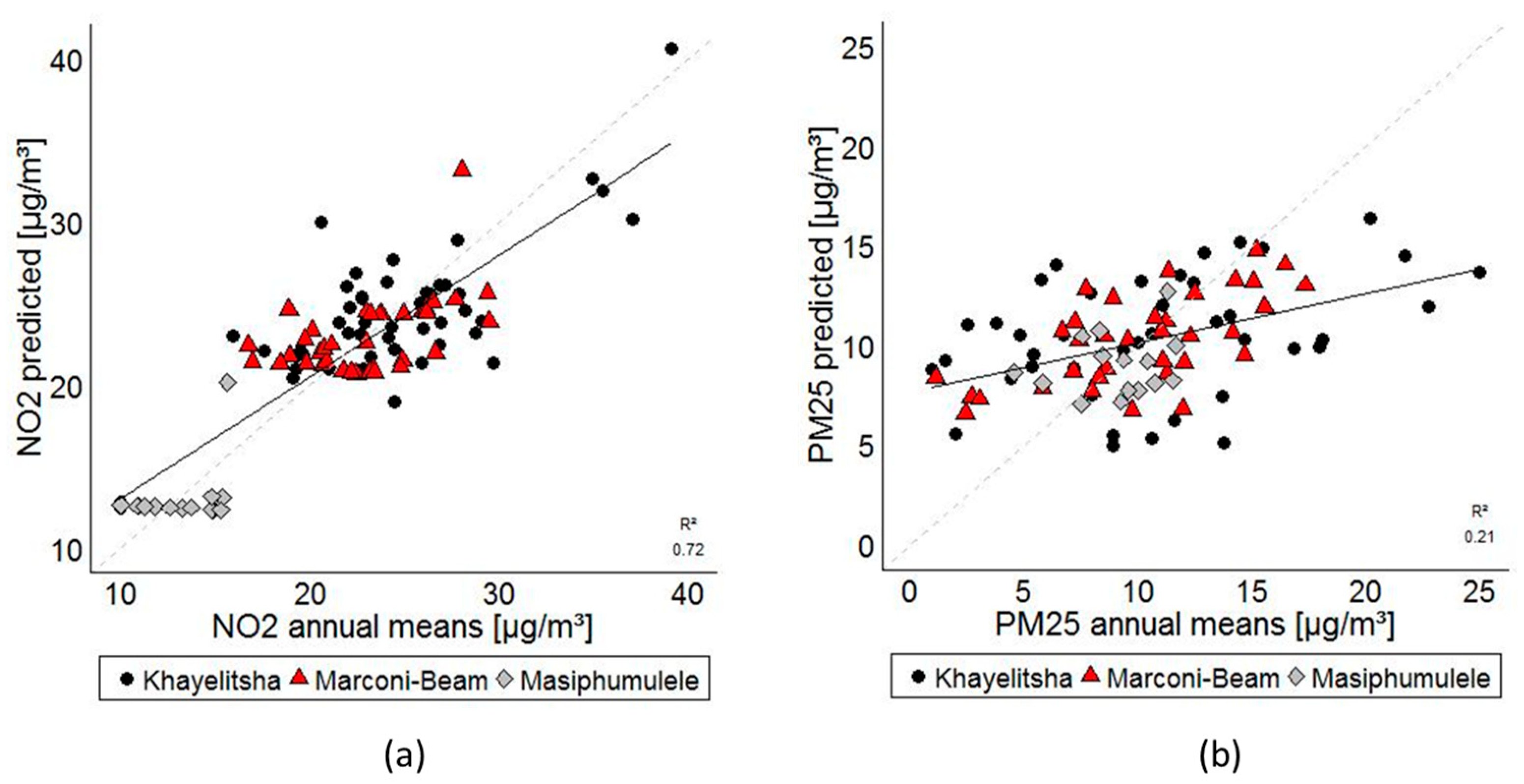
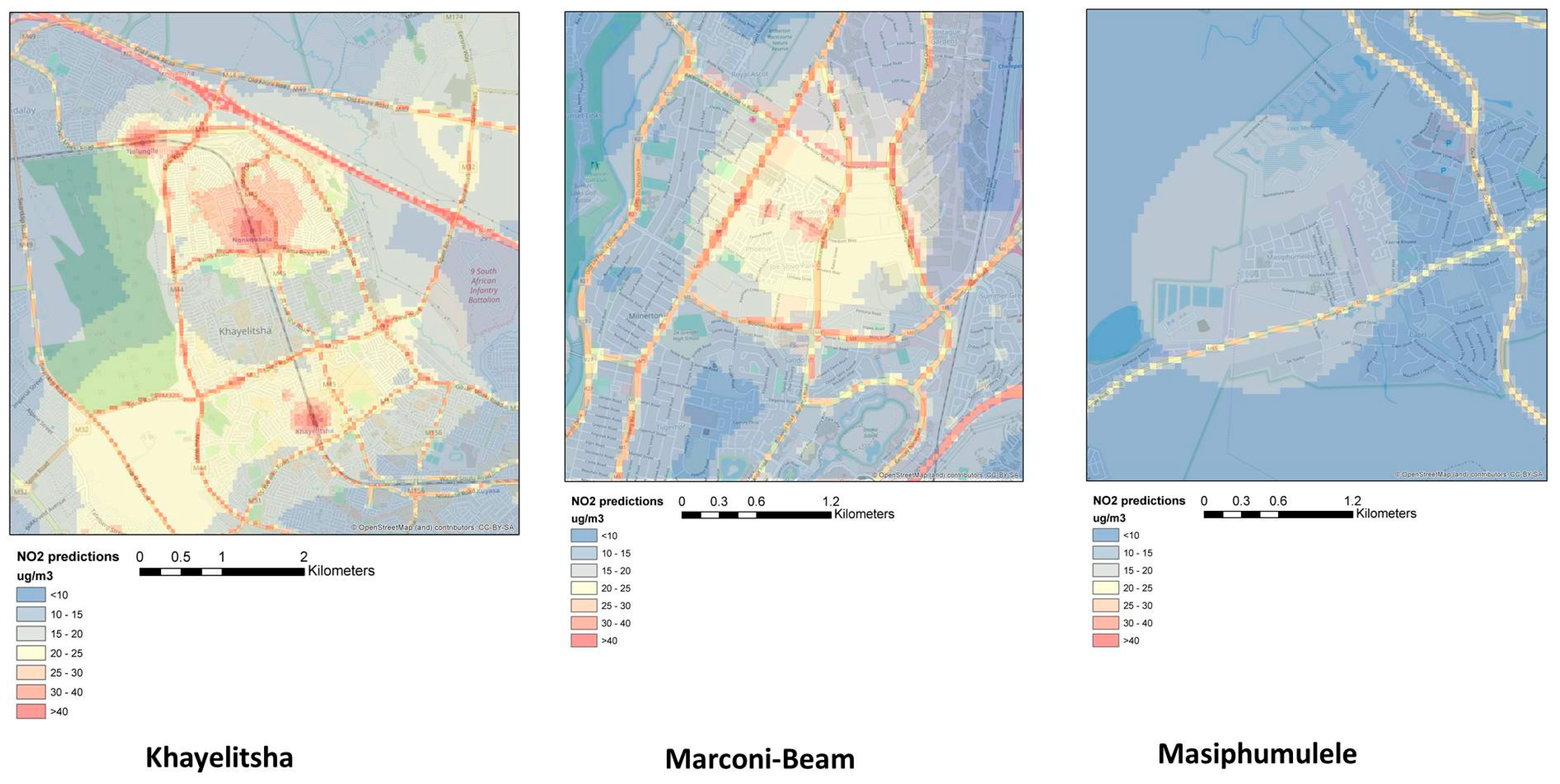
3.4. Validation and Maps
4. Discussion
5. Conclusions
Supplementary Materials
Author Contributions
Funding
Acknowledgments
Conflicts of Interest
References
- Krzyzanowski, M.; Kuna-Dibbert, B.; Schneider, J. Health Effects of Transport-Related Air Pollution; WHO: Geneva, Switzerland, 2005. [Google Scholar]
- WHO. Ambient (Outdoor) Air Quality and Health; WHO: Geneva, Switzerland; Available online: http://www.who.int/mediacentre/factsheets/fs313/en/ (accessed on 6 December 2016).
- WHO. WHO Global Urban Ambient Air Pollution Database (Update 2016); WHO: Geneva, Switzerland, 2016; Available online: http://www.who.int/phe/health_topics/outdoorair/databases/cities/en/ (accessed on 2 May 2017).
- WHO. Ambient Air Pollution: A Global Assessment of Exposure and Burden of Disease; WHO: Geneva, Switzerland, 2016; Available online: http://www.who.int/iris/handle/10665/250141 (accessed on 2 May 2017).
- Air Pollution: Africa’s Invisible, Silent Killer. Available online: http://www.unep.org/stories/Airpollution/Air-Pollution-Africa-Invisible-Silent-Killer.asp (accessed on 30 November 2016).
- Air Quality Management Plan for the Western Cape Province. Department of Environmental Affairs and Development Planning, Provincial Government of the Western Cape. 2010. Available online: http://www.saaqis.org.za/documents/Air%20Quality%20Management%20Plan%20for%20the%20Western%20Cape%20Province.pdf (accessed on 6 September 2016).
- State of Air Quality Management 2015; Western Cape Government, 2015. Available online: https://www.westerncape.gov.za/eadp/sites/eadp.westerncape.gov.za/files/basic-page/downloads/State%20Of%20Air%20Quality%20Monitoring%202015_web.pdf (accessed on 20 February 2018).
- WHO Air Quality Guidelines for Particulate Matter, Ozone, Nitrogen Dioxide and Sulfur Dioxide. Available online: http://apps.who.int/iris/bitstream/10665/69477/1/WHO_SDE_PHE_OEH_06.02_eng.pdf (accessed on 3 January 2017).
- Héroux, M.-E.; Anderson, H.R.; Atkinson, R.; Brunekreef, B.; Cohen, A.; Forastiere, F.; Hurley, F.; Katsouyanni, K.; Krewski, D.; Krzyzanowski, M.; et al. Quantifying the health impacts of ambient air pollutants: Recommendations of a WHO/Europe project. Int. J. Public Health 2015, 60, 619–627. [Google Scholar] [CrossRef] [PubMed]
- Beelen, R. Effects of long-term exposure to air pollution on natural-cause mortality. Lancet 2013, 383, 785–795. [Google Scholar] [CrossRef]
- Coker, E.; Kizito, S. A Narrative Review on the Human Health Effects of Ambient Air Pollution in Sub-Saharan Africa: An Urgent Need for Health Effects Studies. Int. J. Environ. Res. Public Health 2018, 15, 427. [Google Scholar] [CrossRef] [PubMed]
- Ryan, P.H.; LeMasters, G.K. A Review of Land-use Regression Models for Characterizing Intraurban Air Pollution Exposure. Inhal. Toxicol. 2007, 19 (Suppl. 1), 127–133. [Google Scholar] [CrossRef] [PubMed] [Green Version]
- Jerrett, M.; Arain, A.; Kanaroglou, P.; Beckerman, B.; Potoglou, D.; Sahsuvaroglu, T.; Morrison, J.; Giovis, C. A review and evaluation of intraurban air pollution exposure models. J. Expo. Anal. Environ. Epidemiol. 2005, 15, 185–204. [Google Scholar] [CrossRef] [PubMed]
- Hoek, G.; Beelen, R.; de Hoogh, K.; Vienneau, D.; Gulliver, J.; Fischer, P.; Briggs, D. A review of land-use regression models to assess spatial variation of outdoor air pollution. Atmos. Environ. 2008, 42, 7561–7578. [Google Scholar] [CrossRef]
- Gebreab, S.Z.; Vienneau, D.; Feigenwinter, C.; Bâ, H.; Cissé, G.; Tsai, M.-Y. Spatial air pollution modelling for a West-African town. Geospat. Health 2015, 10, 321. [Google Scholar] [CrossRef] [PubMed]
- Muttoo, S.; Ramsay, L.; Brunekreef, B.; Beelen, R.; Meliefste, K.; Naidoo, R.N. Land use regression modelling estimating nitrogen oxides exposure in industrial south Durban, South Africa. Sci. Total Environ. 2018, 610–611, 1439–1447. [Google Scholar] [CrossRef] [PubMed]
- Olaniyan, T.; Jeebhay, M.; Röösli, M.; Naidoo, R.; Baatjies, R.; Künzil, N.; Tsai, M.; Davey, M.; de Hoogh, K.; Berman, D.; et al. A prospective cohort study on ambient air pollution and respiratory morbidities including childhood asthma in adolescents from the Western Cape Province: Study protocol. BMC Public Health. 2017, 17, 712. [Google Scholar] [CrossRef] [PubMed]
- South Africa’s Provinces | South African Government. Available online: http://www.gov.za/about-SA/south-africas-provinces#wc (accessed on 27 November 2016).
- The Housing Development Agency. Western Cape: Informal Settlements Status; The Housing Development Agency: Johannesburg, South Africa, 2013. [Google Scholar]
- Sieber, C.; Ragettli, M.S.; Brink, M.; Toyib, O.; Baatjies, R.; Saucy, A.; Probst-Hensch, N.; Dalvie, M.A.; Röösli, M. Land Use Regression Modeling of Outdoor Noise Exposure in Informal Settlements in Western Cape, South Africa. Int. J. Environ. Res. Public Health 2017, 14, 1262. [Google Scholar] [CrossRef] [PubMed]
- Passam AG. Available online: http://www.passam.ch/products.htm (accessed on 6 December 2016).
- OpenStreetMap. Available online: https://www.openstreetmap.org/ (accessed on 20 December 2016).
- USGS.gov | Science for a Changing World. Available online: https://www.usgs.gov/ (accessed on 20 December 2016).
- Beelen, R.; Hook, G. Exposure Assessment Manual. ESCAPE Project (European Study of Cohorts for Air Pollution Effects). 2010. Available online: http://www.escapeproject.eu/manuals/ESCAPE_Exposure-manualv9.pdf (accessed on 17 May 2017).
- Lawrence, S.; Sokhi, R.; Ravindra, K. Quantification of vehicle fleet PM10 particulate matter emission factors from exhaust and non-exhaust sources using tunnel measurement techniques. Environ. Pollut. 2016, 210, 419–428. [Google Scholar] [CrossRef] [PubMed]
- Hersey, S.P.; Garland, R.M.; Crosbie, E.; Shingler, T.; Sorooshian, A.; Piketh, S.; Burger, R. An overview of regional and local characteristics of aerosols in South Africa using satellite, ground, and modeling data. Atmos. Chem. Phys. 2015, 15, 4259–4278. [Google Scholar] [CrossRef] [PubMed]
- Van der A, R.J.; Eskes, H.J.; Boersma, K.F.; van Noije, T.P.C.; Van Roozendael, M.; De Smedt, I.; Peters, D.H.M.U.; Meijer, E.W. Trends, seasonal variability and dominant NOx source derived from a ten year record of NO2 measured from space. J. Geophys. Res. Atmos. 2008, 113, D04302. [Google Scholar] [CrossRef]
- Beelen, R.; Hoek, G.; Vienneau, D.; Eeftens, M.; Dimakopoulou, K.; Pedeli, X.; Tsai, M.-Y.; Künzli, N.; Schikowski, T.; Marcon, A.; et al. Development of NO2 and NOx land use regression models for estimating air pollution exposure in 36 study areas in Europe—The ESCAPE project. Atmos. Environ. 2013, 72, 10–23. [Google Scholar] [CrossRef]
- Wang, M.; Beelen, R.; Basagana, X.; Becker, T.; Cesaroni, G.; de Hoogh, K.; Dedele, A.; Declercq, C.; Dimakopoulou, K.; Eeftens, M.; et al. Evaluation of Land Use Regression Models for NO2 and Particulate Matter in 20 European Study Areas: The ESCAPE Project. Environ. Sci. Technol. 2013, 47, 4357–4364. [Google Scholar] [CrossRef] [PubMed]
- White, N.; teWaterNaude, J.; van der Walt, A.; Ravenscroft, G.; Roberts, W.; Ehrlich, R. Meteorologically estimated exposure but not distance predicts asthma symptoms in schoolchildren in the environs of a petrochemical refinery: A cross-sectional study. Environ. Health 2009, 8, 45. [Google Scholar] [CrossRef] [PubMed] [Green Version]
- Wichmann, J.; Voyi, K. Ambient Air Pollution Exposure and Respiratory, Cardiovascular and Cerebrovascular Mortality in Cape Town, South Africa: 2001–2006. Int. J. Environ. Res. Public Health 2012, 9, 3978–4016. [Google Scholar] [CrossRef] [PubMed] [Green Version]
- Jerrett, M.; Arain, M.A.; Kanaroglou, P.; Beckerman, B.; Crouse, D.; Gilbert, N.L.; Brook, J.R.; Finkelstein, N.; Finkelstein, M.M. Modeling the intraurban variability of ambient traffic pollution in Toronto, Canada. J. Toxicol. Environ. Health A 2007, 70, 200–212. [Google Scholar] [CrossRef] [PubMed]
- Lee, J.-H.; Wu, C.-F.; Hoek, G.; de Hoogh, K.; Beelen, R.; Brunekreef, B.; Chan, C.C. Land use regression models for estimating individual NOx and NO2 exposures in a metropolis with a high density of traffic roads and population. Sci. Total Environ. 2014. [Google Scholar] [CrossRef] [PubMed]
- Dons, E.; Van Poppel, M.; Int Panis, L.; De Prins, S.; Berghmans, P.; Koppen, G.; Matheeussen, C. Land use regression models as a tool for short, medium and long term exposure to traffic related air pollution. Sci. Total Environ. 2014, 476–477, 378–386. [Google Scholar] [CrossRef] [PubMed]
- Yang, X.; Zheng, Y.; Geng, G.; Liu, H.; Man, H.; Lv, Z.; He, K.; de Hoogh, K. Development of PM2.5 and NO2 models in a LUR framework incorporating satellite remote sensing and air quality model data in Pearl River Delta region, China. Environ. Pollut. 2017, 226, 143–153. [Google Scholar] [CrossRef] [PubMed]
- Moore, D.K.; Jerrett, M.; Mack, W.J.; Künzli, N. A land use regression model for predicting ambient fine particulate matter across Los Angeles, CA. J. Environ. Monit. 2007, 9, 246–252. [Google Scholar] [CrossRef] [PubMed]
- Hoek, G.; Beelen, R.; Kos, G.; Dijkema, M.; van der Zee, S.C.; Fischer, P.H.; Brunekreef, B. Land use regression model for ultrafine particles in Amsterdam. Environ. Sci. Technol. 2011, 45, 622–628. [Google Scholar] [CrossRef] [PubMed]


| Category | GIS Variable Name | Variable Description | Unit | Buffer Radius (m) | Expected Effect |
|---|---|---|---|---|---|
| Roads | MAJROAD | Length of major roads | m | 25/50/100/300/500/1000 | + |
| MAJROAD_d | Distance to nearest major road | m−1; m−2 | + | ||
| ROAD | length of roads (all) | m | 25/50/100/300/500/1000 | + | |
| ROAD_d | Distance to nearest road (all) | m−1; m−2 | + | ||
| Taxi | TAXI | Length of taxi routes | m | 25/50/100/300/500/1000 | + |
| TAXI_d | Distance to nearest taxi route | m−1; m−2 | + | ||
| Bus | BUS_RTE | Length of bus routes | m | 25/50/100/300/500/1000 | + |
| BUS_ST_c | Bus stops | # | 25/50/100/300/500/1000 | + | |
| BUS_ST_d | Distance to nearest bus stop | m−1; m−2 | + | ||
| Rail | RAIL | Length of railways | m | 25/50/100/300/500/1000 | + |
| TRAINSTAT | Distance to nearest train station | m−1; m−2 | + | ||
| Airport | AIR | Distance to nearest airport | m−1; m−2 | + | |
| Point sources | BURN_c | Waste burning sites | # | 25/50/100/300/500/1000 | + |
| BURN_d | Distance to nearest waste burning sites | m−1; m−2 | + | ||
| GRILL_c | Open grills | # | 25/50/100/300/500/1000 | + | |
| GRILL_d | Distance to nearest open grill | m−1; m−2 | + | ||
| CONSTRUCTION | Construction sites | # | 25/50/100/300/500/1000 | + | |
| REFTSTAT_d | Distance to nearest refuse transfer station | m−1; m−2 | + | ||
| Population | INFORMAL | Area of informal settlements | m2 | 25/50/100/300/500/1000 | + |
| ORIGDWELL | Population/building density | # | 25/50/100/300/500/1000 | + | |
| ALLDWELL | Population/building density (from a different source, including informal housings) | # | 25/50/100/300/500/1000 | + | |
| Land use | LU1 | Residential | m2 | 25/50/100/300/500/1000 | + |
| LU2 | Commercial | m2 | 25/50/100/300/500/1000 | + | |
| LU3 | Industrial | m2 | 25/50/100/300/500/1000 | + | |
| LU4 | Open space | m2 | 25/50/100/300/500/1000 | − | |
| LU5 | Vegetation | m2 | 25/50/100/300/500/1000 | − | |
| LU6 | Water bodies | m2 | 25/50/100/300/500/1000 | − | |
| LU7 | Public places | m2 | 25/50/100/300/500/1000 | + | |
| LU8 | Transportation | m2 | 25/50/100/300/500/1000 | + | |
| LU9 | Restauration | m2 | 25/50/100/300/500/1000 | + | |
| Vegetation | NDVI | Normalized Difference Vegetation Index | −1 to +1 | 30/100/150/200/500/750 | − |
| Coast | COAST | Distance to coast | m−1; m−2 | − |
| Poll. | Season | Predictors | Model | LOOCV* | |||||
|---|---|---|---|---|---|---|---|---|---|
| R2* | RMSE* | NMB* | R2* | RMSE* | NMB* | N* | |||
| NO2 | Warm | LU8_1000 + MAJROAD_d + BUS_ST_d + REFSTAT_d + BUS_STOP_500 | 0.62 | 4.8 | −9.9 × 10⁻¹⁶ | 0.57 | 5.1 | −2.5 × 10⁻³ | 94 |
| Cold | GRILL_d + AIR_d + ALLDWELL_1000 +BUS_RTE_300 + REFSTAT_d + BUS_RTE_d | 0.77 | 2.9 | −3.1 × 10⁻³ | 0.72 | 3.2 | −2.1 × 10⁻⁴ | 85 | |
| Annual | MAJROAD_d + BUS_ST_d + GRILL_100 + REFSTAT_d + GRILL_1000 + TRAINSTAT | 0.76 | 2.9 | −3.9 × 10⁻¹⁶ | 0.72 | 3.1 | 2.5 × 10⁻⁴ | 97 | |
| PM2.5 | Warm | RAIL_1000 + GRILL_d + ORIGDWELL_50 + BURN_d + GRILL_500 + REFSTAT_d | 0.36 | 3.1 | 6.4 × 10⁻¹⁷ | 0.26 | 3.3 | −2.1 × 10⁻⁴ | 84 |
| Cold | ALLDWELL_300 + CONSTRUCTION_100 + ORIGDWELL_25 + BUS_RTE_300 + BURN_d | 0.29 | 7.1 | 1.5 × 10⁻¹⁶ | 0.19 | 7.6 | −5.4 × 10⁻³ | 75 | |
| Annual | ALLDWELL_300 + CONSTRUCTION_100 + ORIGDWELL_25 + BURN_d + BUS_RTE_300 | 0.29 | 4.0 | 3.8 × 10⁻¹⁶ | 0.21 | 4.3 | −1.8 × 10⁻³ | 91 | |
© 2018 by the authors. Licensee MDPI, Basel, Switzerland. This article is an open access article distributed under the terms and conditions of the Creative Commons Attribution (CC BY) license (http://creativecommons.org/licenses/by/4.0/).
Share and Cite
Saucy, A.; Röösli, M.; Künzli, N.; Tsai, M.-Y.; Sieber, C.; Olaniyan, T.; Baatjies, R.; Jeebhay, M.; Davey, M.; Flückiger, B.; et al. Land Use Regression Modelling of Outdoor NO2 and PM2.5 Concentrations in Three Low Income Areas in the Western Cape Province, South Africa. Int. J. Environ. Res. Public Health 2018, 15, 1452. https://doi.org/10.3390/ijerph15071452
Saucy A, Röösli M, Künzli N, Tsai M-Y, Sieber C, Olaniyan T, Baatjies R, Jeebhay M, Davey M, Flückiger B, et al. Land Use Regression Modelling of Outdoor NO2 and PM2.5 Concentrations in Three Low Income Areas in the Western Cape Province, South Africa. International Journal of Environmental Research and Public Health. 2018; 15(7):1452. https://doi.org/10.3390/ijerph15071452
Chicago/Turabian StyleSaucy, Apolline, Martin Röösli, Nino Künzli, Ming-Yi Tsai, Chloé Sieber, Toyib Olaniyan, Roslynn Baatjies, Mohamed Jeebhay, Mark Davey, Benjamin Flückiger, and et al. 2018. "Land Use Regression Modelling of Outdoor NO2 and PM2.5 Concentrations in Three Low Income Areas in the Western Cape Province, South Africa" International Journal of Environmental Research and Public Health 15, no. 7: 1452. https://doi.org/10.3390/ijerph15071452