Subsampling of Regional-Scale Database for improving Multivariate Analysis Interpretation of Groundwater Chemical Evolution and Ion Sources

Abstract

Multivariate statistics are widely and routinely used in the field of hydrogeochemistry. Trace elements, for which numerous samples show concentrations below the detection limit (censored data from a truncated dataset), are removed from the dataset in the multivariate treatment. This study now proposes an approach that consists of avoiding the truncation of the dataset of some critical elements, such as those recognized as sensitive elements regarding human health (fluoride, iron, and manganese). The method aims to reduce the dataset to increase the statistical representativeness of critical elements. This method allows a robust statistical comparison between a regional comprehensive dataset and a subset of this regional database. The results from hierarchical Cluster analysis (HCA) and principal component analysis (PCA) were generated and compared with results from the whole dataset. The proposed approach allowed for improvement in the understanding of the chemical evolution pathways of groundwater. Samples from the subset belong to the same flow line from a statistical point of view, and other samples from the database can then be compared with the samples of the subset and discussed according to their stage of evolution. The results obtained after the introduction of fluoride in the multivariate treatment suggest that dissolved fluoride can be gained either from the interaction of groundwater with marine clays or from the interaction of groundwater with Precambrian bedrock aquifers. The results partly explain why the groundwater chemical background of the region is relatively high in fluoride contents, resulting in frequent excess in regards to drinking water standards.

1. Introduction

The goal of multivariate statistical approaches is to discriminate relationships that exist within a dataset of n × m dimensions (i.e., n samples and m chemical elements). For the interpretation of the geochemical origins of groundwater, the purpose is to group samples that share geochemical similarities or to group chemical elements that characterize a group of samples together. Such multivariate techniques are likely to define the intrinsic characteristics of a dataset, as they essentially generate information that helps to formulate hypotheses [1]. However, there are some limitations the user must address to make better use of the multivariate statistical tools.

Truncated distributions are one of the limitations where some data are missing in a dataset (censored data). In geochemistry, such truncations are caused by the detection limit (DL) of the analytical methods. The DL is a function of (1) the analytical apparatus used for the determination of the concentrations of the chemical elements and (2) the purity of the aqueous matrix. Therefore, the DL is not the same, depending on the chemical element analyzed (apparatus), and varies from sample to sample (aqueous matrix).

Censored data (i.e., under the DL) are usually replaced by a single value that is commonly DL/2 [2]. When the amount of data under the DL is high, the DL/2 values significantly impact the correlation factor between two chemical elements. Most multivariate analysis techniques are based on the correlation matrix built from several chemical elements [1,3]. Consequently, the use of the single value DL/2 for the concentration of chemical elements under the DL would induce a bias of results from multivariate analyses. [2] performed data experiments and showed that the performance of the statistical multivariate processing was weakened when the number of substitutions of DL by DL/2 was applied for approximately 30% of the dataset. This phenomenon is referred to as the noise of the analysis [2].

Critical elements that are recognized as sensitive for human health, such as fluoride, barium, manganese, iron, and aluminum [4], commonly fall into this group. These elements may occur in high concentration locally, and are thus of interest for tracking their sources and processes for accounting for their anomalous high concentration.

The objective of this study is to propose a new approach for investigating regional-scale databases of groundwater quality by reducing the impact of censored data for multivariate treatments (i.e., amount of data below DL). The proposed method involves representative subsampling of the regional dataset. Statistical treatments, such as hierarchical Cluster analysis (HCA) and the principal component analysis, were performed on the subset and successfully compared to previous results obtained on the regional-scale database [5]. The subsampling approach generates more accurate treatments with less noise and consequently allows for optimized factorial analysis (FA) for certain chemical parameters of interest. With the subsampling approach, it was possible to better ascertain the evolution of the various types of groundwater and to address the sources of problematic elements, in particular fluorides. The dataset reduction method could be a new method for the study of hydrogeochemical tracers of water-rock interaction mechanisms where the detection limits are still too high to ensure the optimal use of statistical analysis techniques.

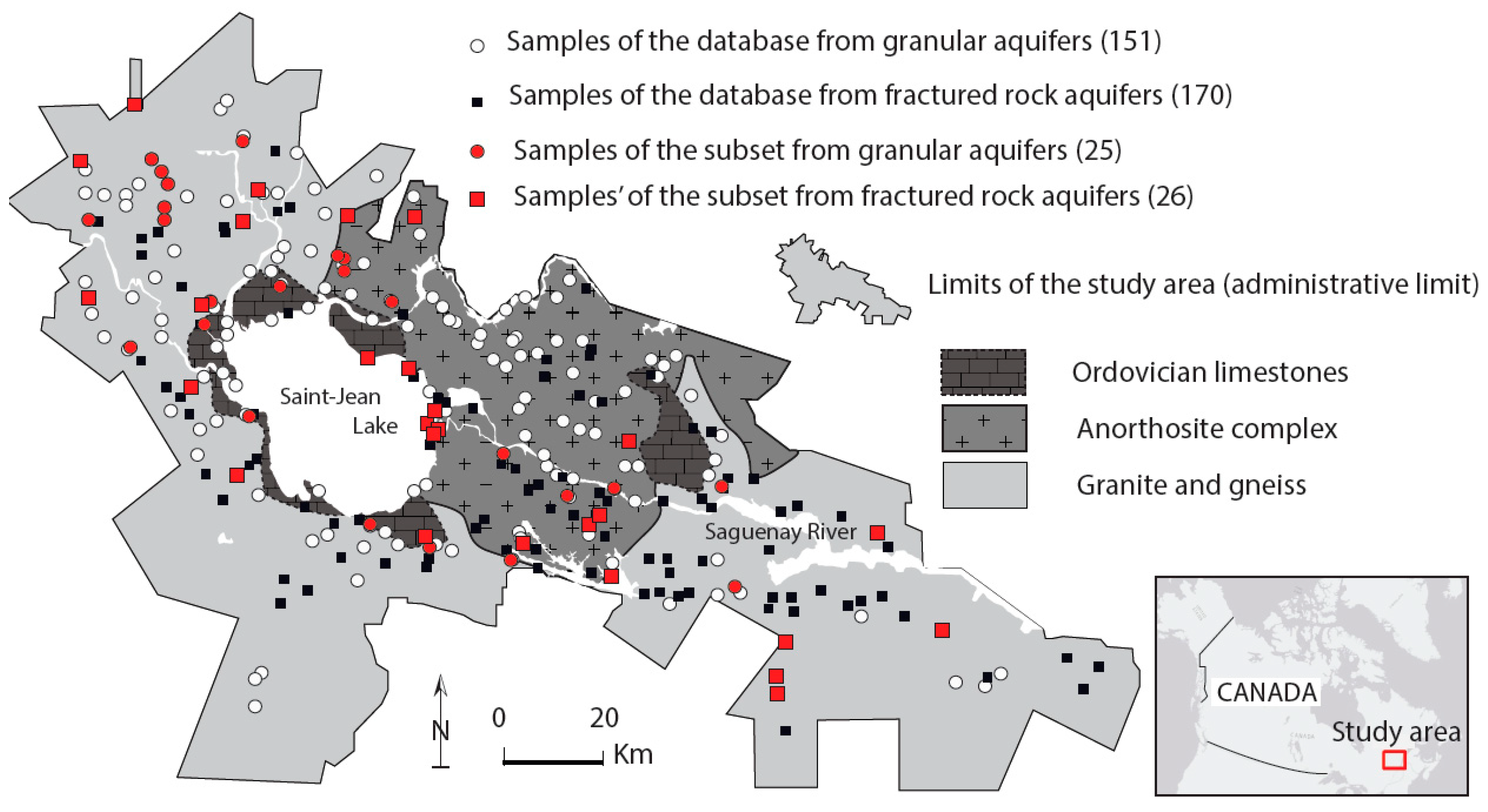
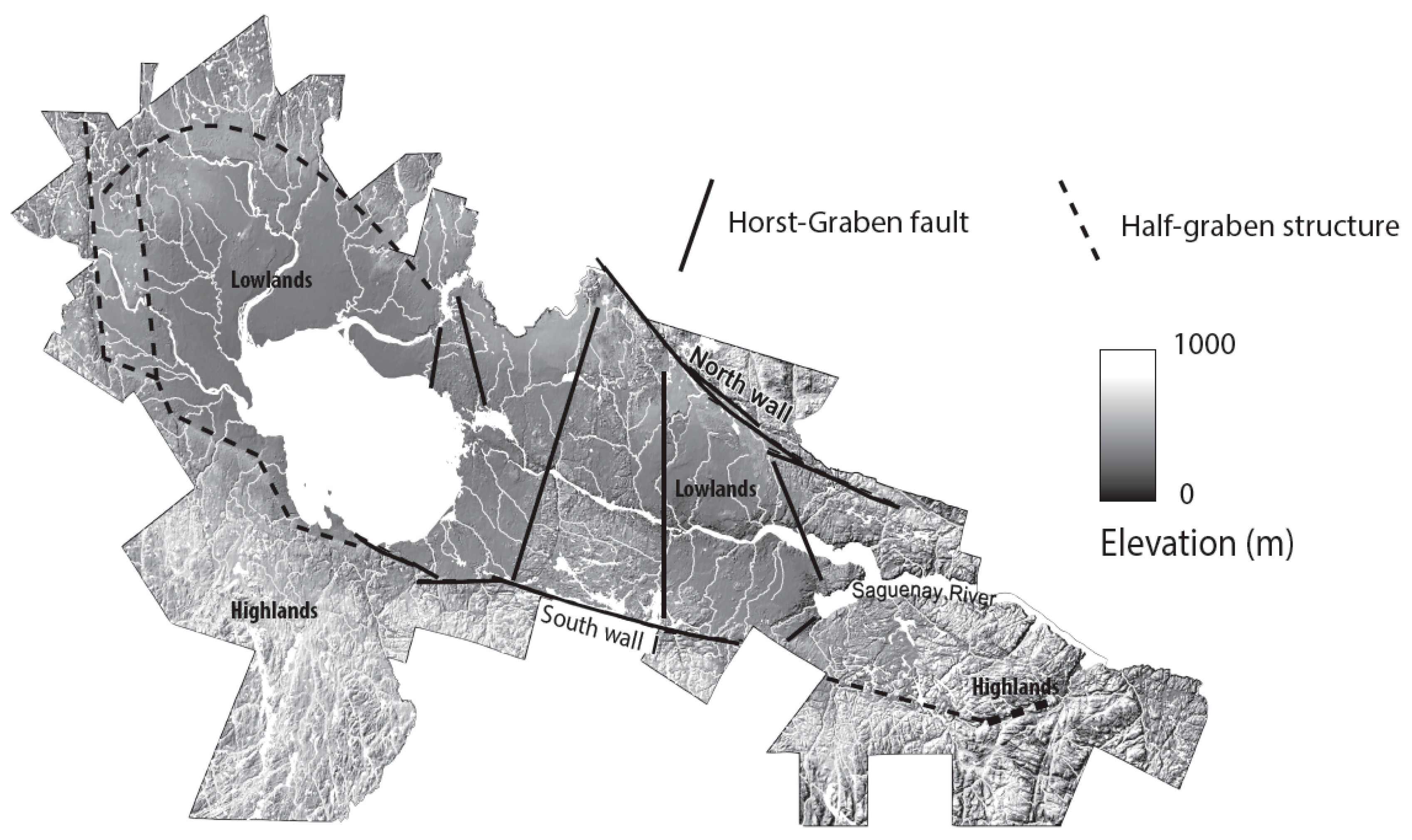
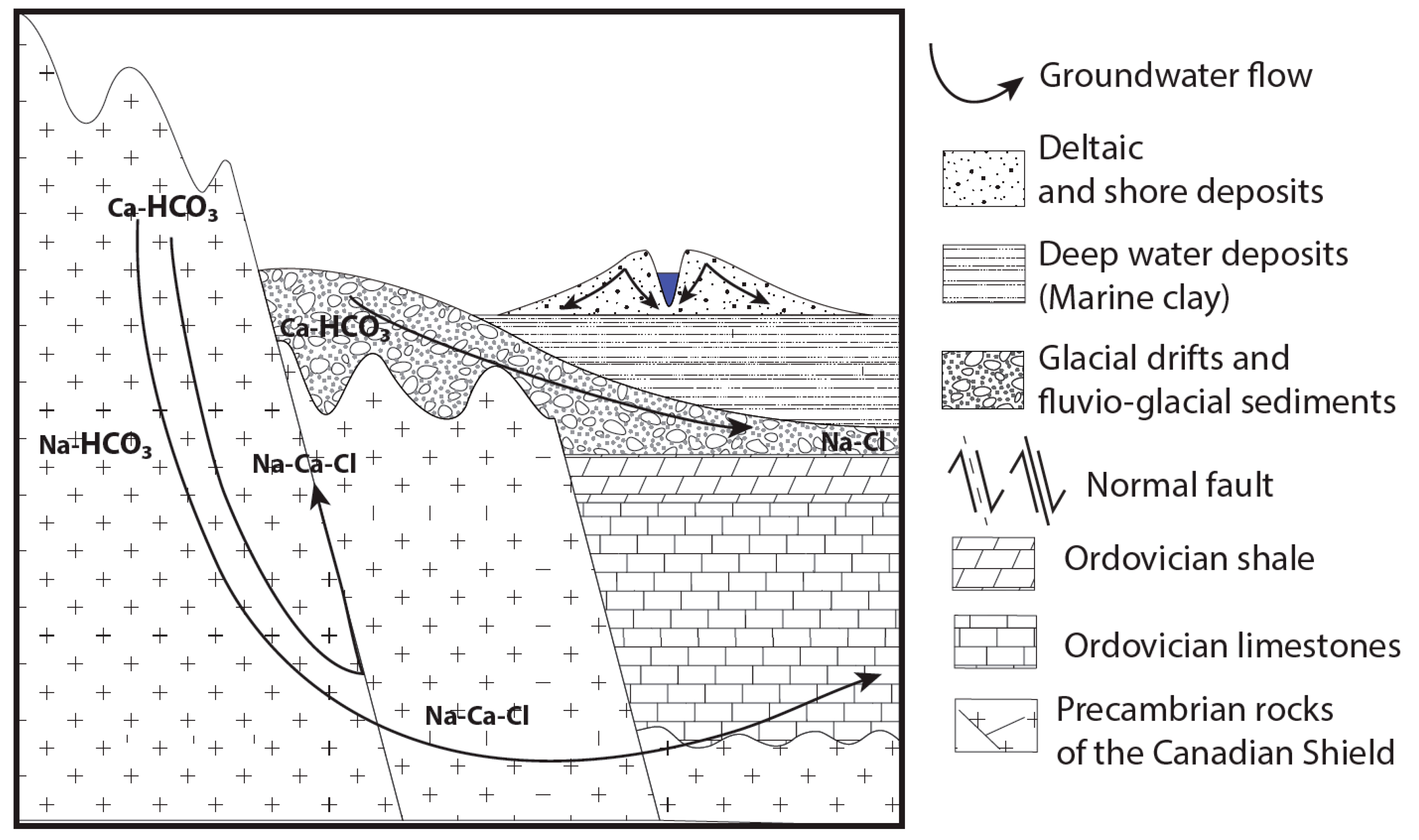
2. Hydrogeological Context

The basement of the Saguenay-Lac-Saint-Jean (SLSJ) region is composed of plutonic rocks belonging to the Precambrian Canadian Shield [6]. Around Lake Saint-Jean and in the lowlands, there are several remnants of an Ordovician platform composed of a series of stratified sedimentary rocks, including siliciclastic strata, micritic limestones, and highly fossiliferous alternating limestones and shales [7] (Figure 1).

The regional topography is controlled by the Phanerozoic Saguenay Graben (180 Ma), which is approximately 30 km wide (Figure 2). The northern and southern walls of the Saguenay Graben are bounded by west-northwest fault systems that mark the limits between the highlands (up to 1000 m asl; rugged terrain dominated by thin glacial drift deposits and outcropping areas) and the lowlands (0 to 200 m asl). The regional physiography has controlled the emplacement and the formation of large accumulations of Quaternary deposits (sand, gravel, and clay-silt) to a thickness of up to 180 m in the central lowlands [8,9], where the most populated areas are located.

When the glaciers retreated approximately 10,000 years ago, the lowlands were invaded by the Laflamme Sea [10]. This marine incursion deposited a semicontinuous extensive layer of deep-water sediments consisting of laminated clayey silt and gray silty clay [11], under which are locally-found confined layers of till, moraines, and eskers [12]. Various facies of deltaic, littoral, and prelittoral sediments were then deposited during the phase of isostatic rebound that forced the retreat of the Laflamme Sea [11,13], and thus, these facies are stratigraphically superimposed on marine deposits. A conceptual cross section presenting the assemblage for the stratigraphic units of the study area, including the highlands/lowlands demarcation, is shown in Figure 3.

According to [5], groundwater mineralization follows two pathways in the SLSJ region (Figure 3). Each of the two salinization paths exerts a major and different influence on the chemical signature of groundwater. First, groundwater in the crystalline bedrock naturally evolves from a recharge-type groundwater to a type of brackish groundwater due to water/rock interactions (plagioclase weathering and mixing with deep basement fluids). Second, the term “water/clay interactions” was introduced to account for a combination of processes: ion exchange, leaching of salt water trapped in the regional aquitard, or both. Mixing with fossil seawater might also increase the groundwater salinity.

Although the groundwater in the SLSJ area is largely of good quality, water with excessive trace element concentrations relative to Canadian drinking water quality guidelines [14], such as fluoride (>1.5 mg/L), barium (>1 mg/L), manganese (>0.05 mg/L), iron (>0.3 mg/L), and aluminum (>0.1 mg/L), have been identified [8]. Fluor are among the chemical elements that have been excluded from the multivariate statistical analysis performed by [5]. Approximately 20% of the samples from the regional-scale dataset have groundwater fluoride levels exceeding the World Health Organization [4] standards [9]. Since Fluoride can have serious health consequences for humans [15], government and municipal authorities are interested in characterizing its source [8].

3. The Statistical Treatment of the Regional Database

Samples were analyzed for a total of 37 elements—major (6), minor (5), and trace elements (26)—from a 321 sample dataset [5]. Figure 1 shows the location of the sampling sites. With conventional statistics, the trace elements, for which at least 30% of the samples have concentrations below the DL, should be removed from the dataset for interpretation (truncated dataset), as suggested [2]. The detection limits for trace elements are such that only 10 chemical elements (K⁺, HCO₃⁻, Mg²⁺, SiO₂, Na⁺, Ca²⁺, Ba²⁺, Sr²⁺, SO₄²⁻, and Mn²⁺) had less than 25% censored data and were considered in the multivariate treatment [5]. The other 23 chemical elements of the regional-scale database were excluded from the multivariate statistical analysis because they had >25% of data below the DL. Therefore, critical elements, such as fluorides, barium, manganese, iron and aluminum, were useless for addressing their source.

4. Methodology

The proposed method aims to reduce the initial dataset to a representative unbiased subgroup to improve the detection ratio of some key chemical elements. The detection ratio is expressed as a percentage of chemical elements above the DL: % NDetected = [NDetected/NDatabase] × 100. The regional-scale database reduction method is based on the current knowledge of the natural evolution of groundwater (i.e., salinization process) of the study area [5], as detailed below.

4.1. Sample Grouping as Hydrogeochemical Poles (RHPs)

In the SLSJ region, the chemistry of groundwater evolves specifically as it flows through the various aquifer types. The regional-scale database was divided into two groups (Figure 1): samples collected in fractured rock aquifers, and samples taken from granular aquifers. Chemical interaction and flow are known to occur simultaneously at all scales of space and time from the surface to the deepest of the porous parts of the continental crust [16,17]. The groundwater chemical evolution can be characterized by considering the water types that are typically found in different zones of groundwater flow systems [18,19,20]. Regardless of the aquifer type, the evolution of the groundwater causes the modification of the bicarbonate-type hydrochemical facies (HCO₃⁻) into a chloride-type hydrochemical facies (Cl⁻). Consequently, the regional-scale database was divided into four groups (i.e., regional hydrogeochemical poles (RHPs)) according to permutation of the water types combined with the two aquifer types. In each of the four groups, samples are selected to form the subset of data by considering the detection ratio for the key chemical elements in each pole. This means that if the detection ratio of a chemical parameter is higher in a subgroup than in the other subgroups, then this chemical parameter characterizes the sub-group.

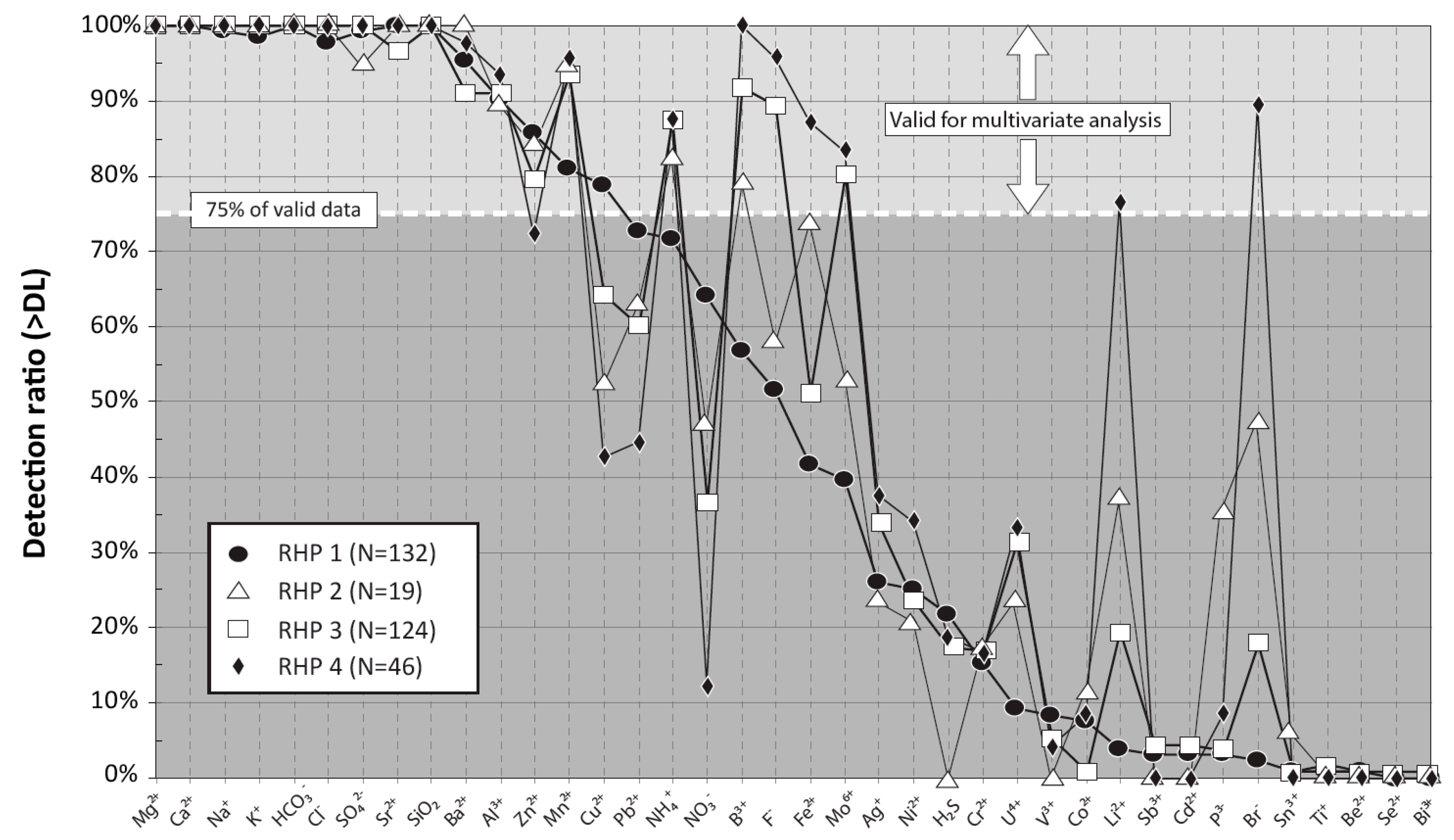
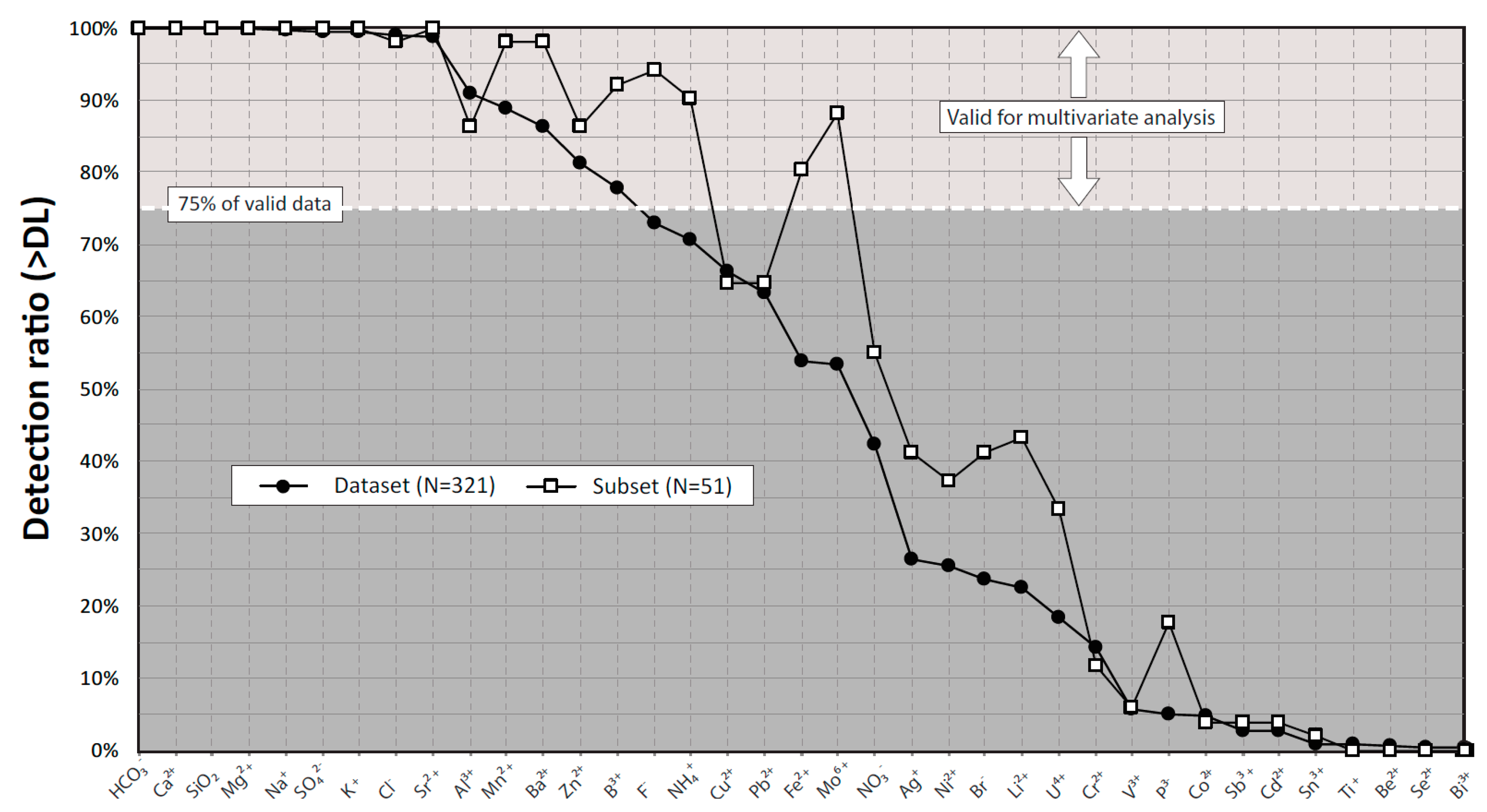
4.2. Detection Ratio of the Key Chemical Elements

Each pole should contain a number of samples that better characterizes them. These samples contain the largest number of key chemical elements with less than 25% of the results below the DL. For each pole, the detection ratios of all the analyzed chemical elements (37 in total) are plotted on a multielement graph and are compared. A greater detection ratio for chemical elements specific to a pole is considered a criterion of representativeness for a given RHP. When the detection ratio of a trace chemical element stands out in an RHP, it is considered a key chemical element. Numerous key chemical elements can characterize an RHP. With key chemical elements identified for a pole, the samples containing the largest number of key chemical elements are selected. The aim is to increase the detection ratio of the key chemical elements until it exceeds the threshold (>25%).

4.3. Multivariate Analysis

The software Statistica version 6.1 [21] was used to perform multivariate statistical analyses. The Box-Cox power transformation [22] was applied to the subset to approximate a normal distribution. The chemical elements were standardized by subtracting the mean concentration of a given element from each measured concentration in the samples of the selected subset and by dividing them by the standard deviation of the distribution [23]. While [2] suggested that the number of analytical values below DL should not exceed 30%, the threshold was lowered to 25% in this study. Consequently, 25% or less of the data below DL were replaced by DL/2.

Hierarchical Cluster analysis produces different Cluster samples, each being characterized by some specific chemical content. With principal component analysis (PCA), the emphasis is on explaining the total variance of the Clusters as linear functions of the chemical elements (i.e., principal components). Factorial analysis (FA) attempts to explain covariances [1] expressed as linear combinations of a small number of highly correlated variables (i.e., the chemical elements). The combinations of variables are called factors.

5. Results

5.1. Identification of the Regional Hydrogeochemical Poles (RHPs)

By combining the two groundwater types (HCO₃⁻ or Cl⁻) and the two aquifer types (bedrock or granular aquifer), the 321 sample dataset was divided into four RHPs: RHP 1: bicarbonate groundwater from granular aquifers (HCO₃_GranAq; 132 samples); RHP 2: chloride groundwater from granular aquifers (Cl_Gran; 19 samples); RHP 3: bicarbonate groundwater from bedrock aquifers (HCO₃_Rock; 124 samples); and RHP 4: chloride groundwater from bedrock aquifers (Cl_Rock; 46 samples). For each RHP, values above the detection limit (N), the median, the first (25) and third (75) quartiles, the maximum (Max), and the minimum (Min) values are presented in

Table 1. Descriptive statistics for the physicochemical parameters of the four regional hydrogeochemical poles defined in this study.

PARAMETER	RHP 1: HCO3_Granular						RHP 2: Cl_Granular						RHP 3: HCO3_Rock						RHP 4: Cl_Rock
	N	Median	25	75	Min	Max	N	Median	25	75	Min	Max	N	Median	25	75	Min	Max	N	Median	25	75	Min	Max
TDS (mg/L)	132	170.2	62.9	282.2	12.1	836.7	19	1167.9	174.4	1679.6	37.3	6107.6	124	291.7	207.7	388.2	62.4	2266.7	46	1862.0	725.4	2857.2	391.3	8266.6
Temperature (Celcius) *	129	8.02	7.02	9.75	4.01	15.60	19	7.83	7.55	9.40	6.47	12.18	124	7.41	6.90	8.13	5.97	13.30	46	7.38	6.92	8.00	4.90	11.30
Redox potential (mV) *	120	97.2	79.7	130.4	−255.7	743.9	17	68.9	−21.2	107.5	−147.0	161.1	104	22.7	−92.0	100.7	−375.6	680.0	43	−12.8	−65.4	78.4	−326.0	720.1
pH *	130	6.98	6.03	7.81	4.38	10.08	19	7.20	5.50	7.61	4.93	8.71	124	7.85	7.06	8.42	4.49	9.74	46	7.64	7.26	7.99	5.18	10.06
Dissolved oxygen (mg/L) *	117	3.62	0.72	7.30	0.00	90.00	17	0.73	0.00	2.76	0.00	6.22	101	0.00	0.00	0.98	0.00	25.10	41	0.05	0.00	0.33	0.00	9.90
Sodium **	131	3.80	1.90	10.00	0.87	240.00	19	220.00	13.00	490.00	3.80	1900.00	124	25.00	7.70	60.00	1.60	840.00	46	315.00	130.00	570.00	20.00	2500.00
Magnesium **	132	2.60	0.95	6.75	0.15	26.00	19	13.40	1.60	25.00	0.31	160.00	124	4.30	2.10	7.20	0.01	26.00	46	15.90	7.80	45.00	3.00	220.00
Potassium **	130	1.30	0.72	2.70	0.14	8.50	19	13.00	1.40	21.00	0.40	64.00	124	1.90	1.30	3.70	0.12	41.00	46	4.50	3.10	18.10	0.54	82.00
Calcium **	132	19.50	7.30	46.00	1.20	130.00	19	21.00	11.00	60.00	2.20	200.00	124	25.00	8.60	48.00	0.04	170.00	46	110.00	44.00	380.00	2.10	1500.00
Bicarbonates *****	132	108.58	32.33	183.00	7.32	427.00	19	207.40	26.84	380.64	6.10	695.40	124	170.80	112.85	219.60	21.52	553.88	46	158.60	117.12	244.00	6.10	683.20
Chloride ***	129	3.40	0.90	10.00	0.16	170.00	19	310.00	55.00	690.00	9.50	3000.00	124	11.00	4.00	35.00	0.07	1100.00	46	815.00	260.00	1600.00	64.00	4200.00
Sulfates ***	131	5.20	3.30	10.00	0.20	41.00	18	44.50	8.60	120.00	2.40	420.00	124	14.00	7.60	18.00	0.10	250.00	46	42.50	15.00	130.00	0.50	530.00
Barium **	126	0.0250	0.0100	0.0500	0.0030	0.3000	19	0.0540	0.0370	0.0800	0.0130	0.6500	112	0.0635	0.0235	0.1250	0.0060	1.2000	46	0.0820	0.0400	0.2200	0.0120	2.8000
Boron **	75	0.0120	0.0073	0.0210	0.0050	0.3500	15	0.2900	0.0160	0.3800	0.0130	0.6600	115	0.0500	0.0240	0.1200	0.0040	3.4000	46	0.2650	0.1400	0.4500	0.0060	1.9000
Strontium **	132	0.0910	0.0390	0.2100	0.0140	2.4000	19	0.3700	0.1500	1.4000	0.0160	7.8000	121	0.2800	0.1100	0.7400	0.0030	4.3000	46	3.750	0.89	13	0.1900	37.0000
Silicium **	132	5.9500	4.7500	7.6500	2.5000	14.0000	19	7.1000	6.0000	9.1000	1.3000	13.0000	124	5.6000	4.9000	6.7000	2.4000	16.0000	46	5.4500	4.6000	7.7000	0.2200	15.0000
Manganese **	107	0.0071	0.0014	0.0530	0.0004	2.4000	18	0.0380	0.0110	0.0710	0.0070	0.2800	117	0.0140	0.0040	0.0420	0.0004	1.0000	44	0.0620	0.0245	0.1020	0.0010	1.1000
Fluoride ****	68	0.2000	0.1000	0.6000	0.1000	2.3000	11	1.3000	0.9000	1.7000	0.1000	2.9000	112	0.8500	0.4000	1.6000	0.1000	4.9000	44	1.3000	0.7100	1.6500	0.0600	3.0000
Aluminium **	119	0.0075	0.0041	0.0180	0.0020	0.1600	17	0.0120	0.0063	0.0290	0.0020	0.1700	114	0.0070	0.0039	0.0097	0.0010	0.2300	43	0.0070	0.0057	0.0120	0.0020	0.0260
Bromide ***	3	0.4000	0.4000	0.5220	0.4000	0.5220	9	4.1050	1.6000	8.0000	1.1000	11.0000	24	0.5000	0.2000	2.0345	0.1000	15.8340	41	7.1000	2.3780	18.0000	0.2000	45.0000
Iron **	55	0.1100	0.0490	0.7800	0.0250	13.0000	14	0.1900	0.1300	1.3000	0.0410	5.4000	65	0.0980	0.0460	0.2400	0.0020	13.0000	40	0.1200	0.0465	0.4100	0.0050	35.0000
Lithium **	5	0.0120	0.0110	0.0130	0.0030	0.0180	7	0.0180	0.0120	0.0300	0.0090	0.0310	26	0.0110	0.0030	0.0150	0.0010	0.6000	35	0.0300	0.0130	0.0700	0.0030	0.5700
Zinc **	113	0.0180	0.0097	0.0540	0.0020	0.7100	16	0.0190	0.0125	0.0500	0.0070	0.1900	98	0.0130	0.0072	0.0250	0.0020	0.3500	34	0.0100	0.0067	0.0120	0.0020	0.1000
Lead **	96	0.0003	0.0002	0.0007	0.0001	0.0073	12	0.0003	0.0002	0.0010	0.0001	0.0021	74	0.0003	0.0002	0.0006	0.0001	0.0020	21	0.0006	0.0003	0.0080	0.0001	0.0100
Ammonium ****	94	0.0600	0.0400	0.1000	0.0200	0.8500	14	0.4650	0.0600	1.1000	0.0400	2.4000	98	0.0950	0.0500	0.2100	0.0200	0.7900	21	0.5100	0.1200	1.6000	0.0300	5.7000
Copper **	104	0.0056	0.0020	0.0130	0.0010	0.3500	10	0.0060	0.0020	0.0390	0.0010	0.0800	79	0.0038	0.0013	0.0120	0.0010	0.2600	20	0.0030	0.0014	0.0100	0.0010	0.0540
Molybdene **	52	0.0015	0.0007	0.0024	0.0010	0.0086	9	0.0020	0.0015	0.0030	0.0010	0.0060	90	0.0019	0.0011	0.0032	0.0010	0.0240	20	0.0020	0.0013	0.0050	0.0010	0.0150
Nickel **	33	0.0018	0.0014	0.0039	0.0010	0.0110	4	0.0020	0.0013	0.0020	0.0010	0.0020	29	0.0019	0.0011	0.0030	0.0010	0.0200	16	0.0020	0.0010	0.0020	0.0010	0.0150
Silver **	34	0.0002	0.0001	0.0003	0.0001	0.0007	4	0.0003	0.0001	0.0003	0.0001	0.0003	38	0.0002	0.0002	0.0003	0.0001	0.0020	9	0.0002	0.0001	0.0010	0.0001	0.0090
Uranium **	12	0.0016	0.0011	0.0022	0.0010	0.0034	4	0.0020	0.0012	0.0020	0.0010	0.0020	35	0.0029	0.0014	0.0055	0.0010	0.0200	8	0.0020	0.0018	0.0030	0.0020	0.0100
Chromium **	20	0.0010	0.0006	0.0014	0.0010	0.0021	3	0.0010	0.0005	0.0010	0.0010	0.0010	19	0.0012	0.0006	0.0016	0.0010	0.0110	4	0.0010	0.0009	0.0020	0.0010	0.0020
Nitrate ***	84	0.3150	0.1000	0.9700	0.0200	8.6000	8	0.8300	0.2500	1.7000	0.0900	3.7000	41	0.2000	0.1000	0.7000	0.0200	4.4000	3	0.11	0.1000	1.2000	0.1000	1.2000
Sulfide ***	5	0.3200	0.3000	0.5900	0.0600	0.7800	0	-	-	-	-	-	8	0.1350	0.0550	0.7050	0.0300	16.0000	3	0.1000	0.0400	1.4000	0.0400	1.4000
Cobalt **	10	0.0023	0.0010	0.0026	0.0010	0.0066	2	0.0010	-	-	-	-	1	0.0013	-	-	-	-	2	0.0010	-	-	-	-
Inorganic phosphorus ****	4	0.1050	0.0550	0.3200	0.0400	0.5000	6	0.0650	0.0500	0.0900	0.0400	0.1100	4	0.3250	0.1750	0.4250	0.0500	0.5000	2	0.0500	-	-	-	-
Vanadium **	11	0.0027	0.0022	0.0042	0.0020	0.0069	0	-	-	-	-	-	6	0.0026	0.0026	0.0031	0.0020	0.0030	1	0.0020	-	-	-	-
Antimony **	4	0.0023	0.0013	0.0042	0.0010	0.0052	0	-	-	-	-	-	5	0.0016	0.0012	0.0020	0.0010	0.0020	0	-	-	-	-	-
Cadmium **	4	0.0003	0.0003	0.0005	0.0002	0.0007	0	-	-	-	-	-	5	0.0006	0.0003	0.0007	0.0003	0.0010	0	-	-	-	-	-
Selenium **	0	-	-	-	-	-	0	-	-	-	-	-	1	0.0420	-	-	-	-	0	-	-	-	-	-
Tin **	1	0.0021	-	-	-	-	1	0.0030	-	-	-	-	1	0.0011	-	-	-	-	0	-	-	-	-	-
Titanium **	1	0.0044	-	-	-	-	0	-	-	-	-	-	2	0.0012	-	-	-	-	0	-	-	-	-	-
Beryllium **	1	0.0044	-	-	-	-	0	-	-	-	-	-	1	0.0008	-	-	-	-	0	-	-	-	-	-
Bismuth **	0	-	-	-	-	-	0	-	-	-	-	-	1	0.0007	-	-	-	-	0	-	-	-	-	-

ANALYTICAL METHODS: * multiparameter probe (in situ); ** Inductively Coupled Plasma Mass Spectrometry (ICP-MS) (mg/L); *** Ion chromatography (mg/L); **** Specific probe (mg/L); ***** Titration (mg/L); 25 and 75 header correspond to the first and the third quantiles; TDS is calculated using the software Aquachem v.5.0; For major, minor and trace elements, data are given in mg/L; If N = 1 or 2: data are underlined; If N = 1: unique measured value is presented; If N = 2: mean value is presented.

.

In Table 1, RHPs of the chloride-type groundwater (advanced stage of hydrochemical evolution; RHP 2 and RHP 4) show a total of dissolved solid (TDS) higher than the TDS of RHPs of the initial hydrochemical evolution stages (bicarbonate type; RHP 1 and RHP 3). Major chemical elements (sodium, magnesium, chlorides, sulfates, and boron) and some of the trace elements (bromides and ammonium) also show higher concentrations in chloride-type groundwater. The highest median for TDS is recorded in the RHPs of the advanced chemical stage of groundwater evolution in fractured rock aquifers (RHP 4). The lowest median for TDS is recorded in the RHPs of the initial chemical evolution stage of groundwater in granular media. Median concentrations for nitrate and phosphorus are higher in the RHP 1 and RHP 3 of the early stage of evolution (HCO₃⁻). In the case of nitrates, the highest median concentration is recorded in groundwater collected from granular aquifers. In the case of phosphorus, the highest median concentration is recorded in groundwater collected in fractured rock aquifers. Overall, Table 1 shows that there are significant differences in the chemical content of RHPs.

The detection ratios of the chemical elements for each of the four RHPs are plotted on a multielement graph (Figure 4). Along the x-axis, ionic species are sorted in descending order of abundance for the most diluted groundwater pole RHP 1 (HCO₃_GranAq); thus, the three other RHPs are “normalized” by the most diluted groundwater endmember. A number of the 10 chemical parameters common to the four RHPs have less than 25% valid data (K⁺, HCO₃⁻, Mg²⁺, SiO₂, Na⁺, Ca²⁺, Ba²⁺, Sr²⁺, SO₄²⁻, and Mn²⁺). These 10 chemical elements can be directly used for further multivariate statistical processing, as was done by [5].

Figure 4 also illustrates that the chemical elements (x-axis) have a different number of detection ratios depending on the RHP where they belong. As observed in Figure 4, bromide (Br⁻) and lithium (Li⁺) present a significant detection ratio in brackish groundwater (RHPs 2 and 4). As presented in Section 4.2, the trace elements with high detection ratios for a given RHP define the key chemical elements; thus, lithium and bromide are considered key chemical elements in RHPs 2 (Cl_Gran) and RHP 4 (Cl_Rock). Nitrates are more frequently detected in groundwater of the bicarbonate type collected in granular aquifers (Figure 4), as well as copper and lead, and are then taken as the key chemical elements for RHP 1 (HCO₃_Gran). Ammonium shows a detection ratio in favor of RHPs 3 and 4 (fractured rock groundwater) and is thus taken as a key chemical element for RHPs 3 and 4. Boron (B³⁺) and molybdenum (Mo⁶⁺) are more frequently detected in brackish groundwater (chloride type; RHPs 2 and 4) and are thus considered key chemical elements in RHPs 2 (Cl_Gran) and RHP 4 (Cl_Rock). The correlation matrices constructed for the four RHPs (Supplementary Materials S1) consistently reveal a strong positive correlation between molybdenum and fluoride. The redox conditions will influence the content of metals with several valences, including iron and manganese. The approach used aims to find the causes of high values in iron and manganese in the groundwater of the region [8]. From Figure 4, manganese already has a detection ratio greater than 75%. Molybdenum, fluoride, and iron were taken as key chemical elements for all RHPs, considering their health importance for the study area. The key chemical elements for each RHP are summarized in

Table 2. Key chemical elements for each regional hydrogeochemical pole (RHP).

Regional Hydrogeochemical Pole (RHP)	Iron	Molybdenum	Fluoride	Nitrates	Copper	Lead	Boron	Bromides	Lithium	Ammonium
RHP 1: Bicarbonate groundwater from granular sediments (HCO3-Gran)	X	X	X	X	X	X
RHP 2: Brackish groundwater from granular sediments (Cl-Gran)	X	X	X				X	X	X
RHP 3: Bicarbonate groundwater from fractured rock (HCO3-Rock)	X	X	X	X						X
RHP 4: Brackish groundwater from fractured rock (Cl-Rock)	X	X	X				X	X	X	X

.

Samples containing the greatest number of key chemical elements are selected according to the proposed approach presented in Section 4. More specifically, the array of analytical results for each sample in each RHP is transformed into a binary matrix, in which the concentrations of chemical elements below the detection limit are replaced by 0, and the analytical results above the detection limit are replaced by 1.

The key chemical elements (Table 2) are weighted by a factor of 10 in the binary matrix. Numbers (replacement values: 0, 1, or 10) are summed for each sample in each RHP. The samples are selected among the best scores in each RHP and are gathered to form the subset.

The final grouping of the samples selected to form the subset has the effect of reducing the detection ratio of some key chemical elements, especially those that are specific to one or two RHPs (Table 2). In the newly formed subset, concentrations above the DL for bromide, lithium, nitrate, copper, and lead could not be increased above the threshold (<25% of data below DL).

As a result, 16 samples were selected for RHP 1, 9 for RHP 2, 16 for RHP 3, and 10 for RHP 4 to form a subset of 51 samples.

Table 3. Statistical data for the 51 sample subset.

	N	%Detect	Median	25	75	Min	Max	Multivariate
TDS (mg/L)	51	100%	427.2	238.3	1359.6	72.0	7291.4
Temperature (Celcius) *	50	98%	7.66	7.13	8.56	5.97	15.60
Redox potential (mV) *	47	92%	79.4	−27.1	101	−245.7	524.9
pH *	50	98%	7.63	7.23	8.09	4.49	10.06
Dissolved oxygen (mg/L) *	38	75%	0.17	0.00	1.82	0.00	8.63
Sodium **	51	100%	40.00	7.50	350.00	1.50	1900.00	x
Magnesium **	51	100%	8.70	3.90	15.00	1.50	160.00	x
Potassium **	51	100%	3.50	2.40	7.50	0.54	64.00	x
Calcium **	51	100%	55.00	21.00	81.00	2.10	1500.00	x
Bicarbonates *****	51	100%	207.40	118.34	280.60	6.10	695.40	x
Chloride ***	50	98%	37.00	6.40	510.00	0.40	4200.00
Sulfates ***	51	100%	18.00	9.20	63.00	1.00	430.00	x
Barium **	50	98%	0.055	0.027	0.110	0.006	0.320	x
Boron **	47	92%	0.120	0.016	0.320	0.006	0.750	x
Strontium **	51	100%	0.400	0.180	1.900	0.033	37.000	x
Silicium **	51	100%	6.500	5.400	8.100	0.220	13.000	x
Manganese **	50	98%	0.031	0.011	0.067	0.001	0.900	x
Fluoride ****	48	94%	0.800	0.300	1.300	0.100	2.400	x
Aluminium **	44	86%	0.007	0.005	0.013	0.002	0.087
Bromide ***	21	41%	3.5000	1.6000	11.0000	0.1000	45.0000
Iron **	41	80%	0.1500	0.0900	0.3600	0.0320	3.4000	x
Lithium **	22	43%	0.0180	0.0120	0.0370	0.0050	0.5700
Zinc **	44	86%	0.0145	0.0077	0.0375	0.0016	0.1500
Lead **	33	65%	0.0004	0.0002	0.0006	0.0001	0.0024
Ammonium ****	46	90%	0.2300	0.0600	0.5100	0.0200	3.0000	x
Copper **	33	65%	0.0027	0.0014	0.0110	0.0006	0.0350
Molybdene **	45	88%	0.0018	0.0014	0.0029	0.0006	0.0150	x
Nickel **	19	37%	0.0019	0.0011	0.0039	0.0010	0.0110
Silver **	21	41%	0.0002	0.0002	0.0003	0.0001	0.0090
Uranium **	17	33%	0.0018	0.0011	0.0054	0.0010	0.0096
Chromium **	6	12%	0.0013	0.0007	0.0018	0.0005	0.0024
Nitrate ***	28	55%	0.3000	0.1000	0.7500	0.0200	6.3000
Cobalt **	2	4%	0.0023	0.0019	0.0026	0.0019	0.0026
Inorganic phosphorus ****	9	18%	0.0500	0.0443	0.0600	0.0400	0.0900
Vanadium **	3	6%	0.0023	0.0023	0.0069	0.0023	0.0069
Antimony **	2	4%	0.0017	0.0014	0.0020	0.0014	0.0020
Cadmium **	2	4%	0.0007	0.0006	0.0007	0.0006	0.0007
Selenium **	0	0%	-	-	-	-	-
Tin **	1	2%	0.0034	-	-	-	-
Titanium **	0	0%	-	-	-	-	-
Beryllium **	0	0%	-	-	-	-	-
Bismuth **	0	0%	-	-	-	-	-

Analytical Methods: * multiparameter probe (in situ); ** Inductively Coupled Plasma Mass Spectrometry; *** Ion chromatography; **** Specific probe; ***** Titration; 25 and 75 header = the first and the third quantiles; TDS is calculated using the software Aquachem v.5.0; For major, minor and trace elements, data are given in mg/L; For the physical parameters, N = number of measured data; For the laboratory analyzed parameters, N = Number of detected values; If N = 1 or 2: data are underlined; If N = 1: unique measured value is presented; If N = 2: mean value is presented; Multivariate header = parameters used in the multivariate analysis.

presents the descriptive statistics (values above the detection limit—N; the median, the first—25; and third—75 quartiles, the maximum—Max; and the minimum—Min) for the 51 samples of the subset. The chemical elements that are used for multivariate statistical processing are shown in bold in Table 3 and marked with a cross in the “Multivariate” column. The physical and chemical data for the subset are presented in

Table 4. Physicochemical data for the Cluster (51 samples of the subset).

Sample	Regional Hydrogeochemical Pole (RHP)	Aquifer Type	Water Type	Detection Limit (DL)					0.03	0.01	0.1	0.05	2	0.5	2	0.001	0.001	0.0001	0.001	0.0002	0.001
				TDS	T	Eh	pH	O.D	Sodium	Magnesium	Potassium	Calcium	Bicarbonate	Chloride	Sulfate	Aluminium	Antimony	Silver	Baryum	Cadmium	Chromium
				(mg/L)		(mV)		(mg/L)	(mg/L)	(mg/L)	(mg/L)	(mg/L)	(mg/L)	(mg/L)	(mg/L)	(mg/L)	(mg/L)	(mg/L)	(mg/L)	(mg/L)	(mg/L)	0.001	0.001	0.0001
1	1	Granular	Ca-HCO3	326.51	6.3	55.7	6.29	UnK	4.2	3.5	2.7	70	207.4	8.6	11	0.0075	-	0.00015	0.026	-	-	Cobalt	Copper	Manganese
2	1	Granular	Ca-HCO3	229.64	11	5.63	4.2	UnK	9.3	11	3.3	24	146.4	5.4	9.4	-	-	0.00018	0.02	-	-	(mg/L)	(mg/L)	(mg/L)
3	1	Granular	Na-HCO3	403.8	13	43.1	5.64	UnK	48	15	5.9	21	256.2	24	18	0.0097	-	0.00016	0.043	-	-	-	0.0007	0.062
4	1	Granular	Ca-HCO3	84.707	7	64.5	5.56	UnK	4.4	2.1	1.3	9.6	51.24	0.4	3.3	0.0095	-	0.00018	0.0055	-	0.0018	-	0.012	0.014
5	1	Granular	Ca-HCO3	459.44	7.6	79.4	8.04	0	40	11	3.1	56	292.8	35	2.1	0.036	0.0014	0.00069	0.055	-	-	-	0.011	0.00081
6	1	Granular	Na-HCO3	217.36	9.8	88.7	8.22	0	16	8.7	7.1	15	146.4	4.3	3.5	0.0022	-	-	0.05	-	-	-	0.0092	0.00089
7	1	Granular	Ca-HCO3	427.22	6.9	90.6	7.73	1.7	3.6	11	3.9	81	268.4	6.4	41	0.003	-	-	0.14	-	-	-	0.0009	0.042
8	1	Granular	Ca-HCO3	335.39	6.6	90.2	8.01	8.63	4	6.1	2.5	64	219.6	4.8	25	-	-	-	0.08	-	-	-	-	0.021
9	1	Granular	Ca-HCO3	247.93	6.8	98.9	7.57	8.48	13	14	4.8	21	170.8	1.1	5	0.0039	-	0.0001	0.031	-	-	-	0.0027	0.039
10	1		Ca-HCO3	228.6	6	91.6	8.33	0	13	11	5.6	24	134.2	14	9.2	0.0044	-	0.00012	0.078	-	-	-	-	0.015
11	1	Granular	Ca-HCO3	396.69	7.1	120.4	7.39	3.33	7.6	10	2.4	76	256.2	9.1	23	0.022	-	0.0001	0.027	-	-	-	0.016	0.011
12	1	Granular	Ca-HCO3	200.13	7.7	116.4	7.63	2.85	9.5	9.7	3.6	23	118.34	8.3	10	0.0088	-	-	0.017	-	-	-	0.0009	0.033
13	1	Granular	Ca-HCO3	311.59	8.1	97.8	7.49	0.77	13	8.2	3.5	46	207.4	9.6	7	0.0053	-	-	0.055	-	-	-	0.0059	0.03
14	1	Granular	Ca-HCO3	238.27	9.1	UnK	7.67	2.45	1.5	3	0.77	55	170.8	1.4	5.8	0.002	-	-	0.058	-	0.00071	-	0.0019	0.0024
15	1	Granular	Ca-HCO3	454.73	9.1	−75	6.93	0.72	7.5	15	5.6	84	280.6	16	30	0.0063	-	0.00014	0.06	-	-	-	0.015	0.032
16	1		Ca-HCO3	463.85	16	6.4	6.84	1.57	5.6	4	7.5	110	305	2.6	12	0.022	-	-	0.094	-	-	-	0.0012	0.094
17	2	Granular	Na-Cl	5573.4	7.5	27.9	6.47	UnK	1600	100	55	60	695.4	2700	330	0.0046	-	0.00016	0.039	-	-	0.0026	0.0006	0.9
18	2	Granular	Na-Cl	1359.6	9.5	−21.2	7.31	UnK	350	13	13	9.8	536.8	340	79	0.012	-	0.00028	0.029	-	0.00098	0.0019	0.0035	0.66
19	2	Granular	Na-Cl	3576	7.8	−132	7.61	0.73	980	52	21	150	317.2	1900	120	0.0021	-	0.00033	0.25	-	-	-	-	0.071
20	2	Granular	Na-Cl	1352.8	7.8	104.9	8.1	0	220	15	11	200	183	630	63	0.02	-	-	0.07	-	-	-	0.0011	0.031
21	2	Granular	Na-Cl	1387.7	7.5	107.5	8.71	0	410	18	14	19	207.4	570	130	0.013	-	-	0.053	-	-	-	-	0.055
22	2	Granular	Na-Cl	1679.6	7.6	−147	7.41	0	490	20	34	36	341.6	690	68	0.087	-	-	0.094	-	-	-	-	0.061
23	2	Granular	Na-Cl	6107.6	7.6	−97.9	7.2	0	1900	160	64	100	463.6	3000	420	-	-	-	0.064	-	0.00052	-	-	0.011
24	2	Granular	Na-Cl	2709.1	9.4	−8.3	8.09	0	830	33	31	58	380.64	1100	250	0.007	0.0005	-	0.06	-	-	-	-	0.15
25	2	Granular	Na-Cl	1283.2	9.4	−75.3	8.47	0.11	370	13.4	15	21	353.8	390	100	0.007	0.0005	-	0.043	-	-	-	-	0.098
26	3	Rock	Ca-HCO3	125.52	11	133.5	4.7	UnK	4.3	2.1	2.5	23	70.76	3	4.8	0.0076	-	-	0.022	-	-	-	0.002	0.067
27	3	Rock	Ca-HCO3	372.21	7.9	95.2	5.58	UnK	25	7.2	2.8	60	231.8	10	26	0.0096	-	0.00029	0.16	-	-	-	-	0.018
28	3	Rock	Ca-HCO3	72.019	7.9	100.5	4.49	UnK	2.1	1.5	0.92	11	40.26	-	4	0.0095	-	0.00041	0.018	-	-	-	0.026	0.0025
29	3	Rock	Ca-HCO3	229.08	6.6	42.5	6.02	UnK	21	6.3	2.4	25	102.48	45	12	0.023	-	0.00021	0.087	-	0.0017	-	0.029	0.0087
30	3	Rock	Ca-HCO3	393.04	6.3	−182	7.55	0	20	6.7	2.8	71	207.4	45	25	0.0072	-	0.00018	0.11	0.00061	-	-	0.035	0.0094
31	3	Rock	Ca-HCO3	153.57	6	524.9	8.06	0.22	5.4	4.3	1	24	104.92	0.5	1.1	0.007	-	-	0.015	-	-	-	0.0049	0.038
32	3	Rock	Ca-HCO3	322.78	8.8	UnK	7.44	5.59	5.5	7.5	2.9	58	219.6	5.1	13	0.0048	0.002	-	0.12	-	-	-	0.028	0.015
33	3	Rock	Na-HCO3	474.48	7.7	93	8.64	0	110	3	3	10	292.8	22	18	0.017	-	-	0.037	-	-	-	0.0034	0.048
34	3	Rock	Na-HCO3	512.36	7.3	111.5	8.01	0	140	2.6	3.3	7.1	256.2	65	24	0.0078	-	-	0.03	-	-	-	0.0098	0.0019
35	3	Rock	Ca-HCO3	162.56	7.8	101.5	6.19	6.46	7.5	3.9	1.5	28	69.54	19	13	0.0092	-	-	0.047	0.00073	-	-	-	0.013
36	3	Rock	Ca-HCO3	92.998	7.1	101	7.83	0.9	2.5	2.8	2.1	11	50.02	0.5	6.3	0.0067	-	-	0.018	-	-	-	-	0.0035
37	3	Rock	Ca-HCO3	304.9	7.2	307.2	7.53	4.73	8.4	6.8	1.8	63	207.4	3.5	14	-	-	0.00016	0.13	-	-	-	0.01	0.0043
38	3	Rock	Ca-HCO3	508.64	UnK	UnK	UnK	UnK	47	12	3.7	77	195.2	110	45	0.058	-	-	0.065	-	-	-	0.002	0.0041
39	3	Rock	Ca-HCO3	207.73	7.3	−98.9	8.21	1.18	20	5.7	1.4	26	111.02	16	15	0.0054	-	-	0.24	-	-	-	0.0025	0.013
40	3	Rock	Na-HCO3	497.36	8.6	UnK	8.06	0	130	3	5.3	7.3	256.2	64	16	0.02	-	-	0.015	-	-	-	0.002	0.065
41	3	Rock	Na-HCO3	401.03	7.7	58.1	8.54	0.87	100	1.9	4.4	4.7	231.8	39	3.3	-	-	-	-	-	-	-	0.014	0.009
42	4	Rock	Na-Cl	498.99	7.3	−29.9	7.62	UnK	110	7.8	3.2	32	134.2	170	25	0.0029	-	0.0012	0.32	-	-	-	0.0014	0.013
43	4	Rock	Ca-Cl	630.02	6.6	−27.1	7.72	UnK	75	3.3	0.54	130	104.92	280	9.5	0.0028	-	-	0.22	-	-	-	-	0.015
44	4	Rock	Ca-Cl	5227.9	8.5	−246	8.6	0	570	3	1.6	1500	6.1	3000	53	0.0035	-	-	0.26	-	-	-	-	0.025
45	4	Rock	Ca-Cl	2113.4	9.2	82.9	7.78	0	260	60	4.5	400	231.8	1000	110	0.026	-	0.0002	0.16	-	-	-	-	0.19
46	4	Rock	Ca-Cl	590.73	7.4	91.1	8.53	0	84	17	1.6	94	104.92	230	45	0.0037	-	-	0.054	-	-	-	0.0015	0.11
47	4	Rock	Ca-Cl	391.26	6.7	129.6	7.54	7.55	45	3.9	0.65	62	117.12	110	40	-	-	-	0.018	-	-	-	0.0006	0.046
48	4	Rock	Na-Cl	1794.8	7.3	102.5	10.1	0	560	12	20	2.1	683.2	510	1	0.0048	-	0.009	0.012	-	-	-	-	0.081
49	4	Rock	Ca-Cl	2857.2	8.4	−102	7.82	0	380	54	3.6	580	158.6	1600	81	0.0072	-	-	0.18	-	-	-	-	-
50	4	Rock	Na-Cl	7291.4	7.8	−21.8	7.59	1.82	1800	140	16	520	134.2	4200	420	0.0091	-	0.00015	0.2	-	0.0024	-	0.0012	0.0092
51	4	Rock	Na-Cl	6301	7.2	−100	7.23	0	1900	160	64	120	427	3200	430	-	-	-	0.024	-	-	-	0.0026	0.077
Sample	Regional Hydrogeochemical Pole (RHP)	Aquifer Type	Water Type	0.001	0.001	0.002	0.004	0.001	0.01	0.01	0.002	0.001	0.001	0.002	0.001	0.001	0.1	0.0001	0.001	0.02	0.1	0.1	0.1	0.04
				Molybdenum	Nickel	Zinc	Boron	Iron	Lithium	Selenium	Strontium	Tin	Titan	Vanadium	Berillium	Bismuth	Silicium	Lead	Uranium	Amonium	Bromide	Fluoride	Nitrate	Phosphorus
				(mg/L)	(mg/L)	(mg/L)	(mg/L)	(mg/L)	(mg/L)	(mg/L)	(mg/L)	(mg/L)	(mg/L)	(mg/L)	(mg/L)	(mg/L)	(mg/L)	(mg/L)	(mg/L)	(mg/L)	(mg/L)	(mg/L)	(mg/L)	(mg/L)
1	1	Granular	Ca-HCO3	0.0006	-	0.0073	-	0.062	-	-	0.19	-	-	-	-	-	6.2	0.00031	-	0.05	-	-	6.3	-
2	1	Granular	Ca-HCO3	0.0006	-	0.058	0.01	0.14	0.013	-	0.21	-	-	-	-	-	9.6	0.00022	-	0.06	-	0.2	0.9	-
3	1	Granular	Na-HCO3	0.0031	-	0.012	0.068	-	-	-	0.27	-	-	-	-	-	7.1	0.00041	0.001	0.08	-	0.7	0.3	-
4	1	Granular	Ca-HCO3	0.00087	-	0.055	0.011	-	-	-	0.033	-	-	0.0023	-	-	5.7	0.0014	-	0.04	-	0.6	0.2	-
5	1	Granular	Ca-HCO3	-	-	0.004	0.13	0.78	0.018	-	0.96	-	-	-	-	-	8.1	0.00016	-	0.51	-	0.4	-	-
6	1	Granular	Na-HCO3	0.003	-	0.0021	0.011	0.13	-	-	0.14	-	-	-	-	-	7.7	0.00014	-	0.28	-	0.3	0.02	-
7	1	Granular	Ca-HCO3	0.0018	0.0029	0.0052	0.0055	1.1	-	-	0.2	-	-	-	-	-	5.1	0.00049	-	0.02	-	0.2	-	-
8	1	Granular	Ca-HCO3	0.0013	0.0021	-	0.011	0.11	-	-	0.17	-	-	-	-	-	4.4	-	-	-	-	0.1	0.1	-
9	1	Granular	Ca-HCO3	0.0017	0.011	0.015	0.015	-	-	-	0.16	-	-	-	-	-	8.6	0.00051	-	0.07	-	0.2	0.5	-
10	1		Ca-HCO3	0.0029	-	0.0023	0.016	0.081	-	-	0.35	-	-	-	-	-	8	0.00022	-	0.23	-	0.8	-	-
11	1	Granular	Ca-HCO3	0.0015	0.0019	0.017	0.014	-	-	-	0.21	-	-	-	-	-	5.7	0.00023	-	0.05	-	0.1	0.51	-
12	1	Granular	Ca-HCO3	0.00075	-	0.024	0.0072	0.3	-	-	0.16	-	-	-	-	-	8.1	-	-	0.07	-	0.1	0.8	-
13	1	Granular	Ca-HCO3	0.0021	0.0016	0.026	0.015	3.4	-	-	0.14	-	-	-	-	-	6.3	-	0.0011	-	-	0.3	0.3	-
14	1	Granular	Ca-HCO3	0.00083	-	-	0.02	2.4	-	-	0.14	-	-	-	-	-	5.7	-	-	0.05	-	0.2	0.02	-
15	1	Granular	Ca-HCO3	0.0022	0.0031	0.09	0.017	2	-	-	0.31	-	-	-	-	-	6.1	0.0002	-	0.34	-	0.1	-
16	1		Ca-HCO3	-	0.0042	0.072	0.025	0.21	-	-	0.46	-	-	0.0069	-	-	6.5	0.00015	-	0.4	-	0.1	2.1	-
17	2	Granular	Na-Cl	0.0015	0.0016	0.044	0.57	0.19	0.018	-	1.4	-	-	-	-	-	8.8	-	0.0018	2.2	10	0.9	-	-
18	2	Granular	Na-Cl	0.0044	-	0.026	0.36	0.13	-	-	0.19	-	-	-	-	-	6.9	0.00021	0.0021	0.47	1.1	1.8	-	0.07
19	2	Granular	Na-Cl	0.0016	0.0011	0.015	0.38	1	0.031	-	5.8	-	-	-	-	-	9.1	0.00019	-	1.4	7	1.7	-	0.05
20	2	Granular	Na-Cl	0.0028	-	0.0066	0.17	0.29	0.012	-	7.8	-	-	-	-	-	6.5	-	0.0011	0.41	8	1	-	-
21	2	Granular	Na-Cl	0.0055	-	0.15	0.19	0.19	-	-	0.71	-	-	-	-	-	6.7	0.0001	-	0.81	1.6	1.7	0.46	-
22	2	Granular	Na-Cl	0.00056	-	0.0092	0.29	3.1	0.017	-	0.49	-	-	-	-	-	9.2	-	-	0.46	2.8	0.7	-	0.09
23	2	Granular	Na-Cl	0.0015	-	-	0.66	1.3	0.03	-	2.9	-	-	-	-	-	13	-	0.0012	2.4	11	1.1	-	0.04
24	2	Granular	Na-Cl	0.003	-	0.014	0.6	0.19	0.02	-	1.9	-	-	-	-	-	9.1	-	0.0011	1.1	4.1	1.3	0.074	-
25	2	Granular	Na-Cl	0.003	-	0.011	0.36	0.047	0.009	-	0.98	-	-	-	-	-	7.7	-	0.0011	1.1	1.4	1.6	0.074	-
26	3	Rock	Ca-HCO3	-	-	0.052	-	0.046	-	-	0.068	-	-	-	-	-	5.6	0.001	-	0.03	-	0.1	3.5	-
27	3	Rock	Ca-HCO3	0.00099	0.0012	0.0086	0.12	-	-	-	1.2	-	-	-	-	-	3.4	0.00067	-	0.06	-	0.8	0.21	-
28	3	Rock	Ca-HCO3	-	-	0.038	0.0086	0.12	-	-	0.18	-	-	-	-	-	5.6	0.00042	-	0.32	-	0.2	0.1	-
29	3	Rock	Ca-HCO3	0.002	0.0011	0.014	0.024	0.09	-	-	0.33	-	-	-	-	-	6.8	0.00045	-	0.09	-	0.6	-	-
30	3	Rock	Ca-HCO3	0.0011	0.0039	0.028	0.03	0.32	-	-	0.72	-	-	-	-	-	6.7	0.00032	-	0.08	-	0.4	-	-
31	3	Rock	Ca-HCO3	0.008	0.0012	0.036	0.021	0.032	-	-	0.23	-	-	-	-	-	5.5	0.00041	0.0013	0.05	-	0.9	-	-
32	3	Rock	Ca-HCO3	-	-	0.0081	-	0.071	-	-	0.43	-	-	-	-	-	4.9	0.00047	-	0.03	-	-	0.7	-
33	3	Rock	Na-HCO3	0.0015	-	-	0.18	0.12	-	-	0.4	-	-	-	-	-	6.1	-	0.0054	0.29	0.1	2.3	0.02	0.05
34	3	Rock	Na-HCO3	0.0027	-	-	0.14	0.032	-	-	0.28	-	-	-	-	-	5.3	0.0024	0.0089	0.06	0.2	2.3	0.5	-
35	3	Rock	Ca-HCO3	-	0.0011	0.037	-	0.033	-	-	0.18	-	-	-	-	-	8.3	0.00055	-	-	-	-	3.2	-
36	3	Rock	Ca-HCO3	0.002	-	0.012	0.011	0.043	-	-	0.041	-	-	0.0023	-	-	8.5	0.00029	-	0.04	-	0.4	0.2	-
37	3	Rock	Ca-HCO3	0.0029	-	0.011	0.022	-	-	-	2	-	-	-	-	-	6.1	0.00088	0.0054	0.05	-	1.7	1.7	-
38	3	Rock	Ca-HCO3	0.0018	0.0021	0.02	0.057	0.36	-	-	1.6	-	-	-	-	-	7.1	0.00043	-	0.11	-	1	-	-
39	3	Rock	Ca-HCO3	0.0012	0.0058	0.032	0.042	-	-	-	2.2	-	-	-	-	-	4.5	0.002	-	0.16	-	0.8	0.1	-
40	3	Rock	Na-HCO3	0.0029	0.0039	0.011	0.3	-	-	-	0.16	-	-	-	-	-	6.7	0.00058	0.0055	0.23	-	1.3	0.1	-
41	3	Rock	Na-HCO3	0.00065	-	0.13	0.46	0.19	0.011	-	0.077	-	-	-	-	-	6.5	-	-	0.45	-	1.2	0.4	-
42	4	Rock	Na-Cl	0.0016	-	-	0.25	0.066	0.013	-	1.4	-	-	-	-	-	5.6	0.00019	-	0.51	2	1	-	-
43	4	Rock	Ca-Cl	0.0078	-	0.0041	0.22	0.15	0.07	-	4.1	-	-	-	-	-	8.2	-	0.0019	-	3.5	1.9	-	-
44	4	Rock	Ca-Cl	0.0065	-	0.012	0.14	0.7	0.57	-	37	-	-	-	-	-	4.5	-	-	0.12	45	1.3	-	-
45	4	Rock	Ca-Cl	0.0017	0.001	0.0029	0.32	0.1	0.084	-	18	-	-	-	-	-	5.2	0.0015	-	1.7	15	1.3	-	0.06
46	4	Rock	Ca-Cl	0.0036	-	0.0016	0.15	0.13	0.014	-	2.3	-	-	-	-	-	3.4	0.00011	0.0036	0.07	3	1.6	-	-
47	4	Rock	Ca-Cl	0.0015	-	0.0041	0.037	-	0.021	-	0.69	-	-	-	-	-	5.4	-	0.0096	-	0.2	0.7	0.11	-
48	4	Rock	Na-Cl	0.006	0.001	0.0067	0.35	0.15	0.01	-	0.22	-	-	-	-	-	0.22	-	-	1.8	1.9	1.6	-	-
49	4	Rock	Ca-Cl	0.0059	-	0.064	0.75	-	0.082	-	22	-	-	-	-	-	5	0.00062	-	1.3	24	2.4	-	-
50	4	Rock	Na-Cl	0.015	-	0.1	0.46	0.27	0.12	-	27	-	-	-	-	-	4.8	-	-	3	19	0.8	-	0.04
51	4	Rock	Na-Cl	0.0014	-	-	0.68	1.3	0.037	-	3.7	-	-	-	-	-	11	-	0.0016	2.8	12	1.1	-	-

. The 51 samples have a good distribution over the study area (Figure 1). The ionic concentrations of the subset are compared to the one of the regional-scale databases in Section 5.2.

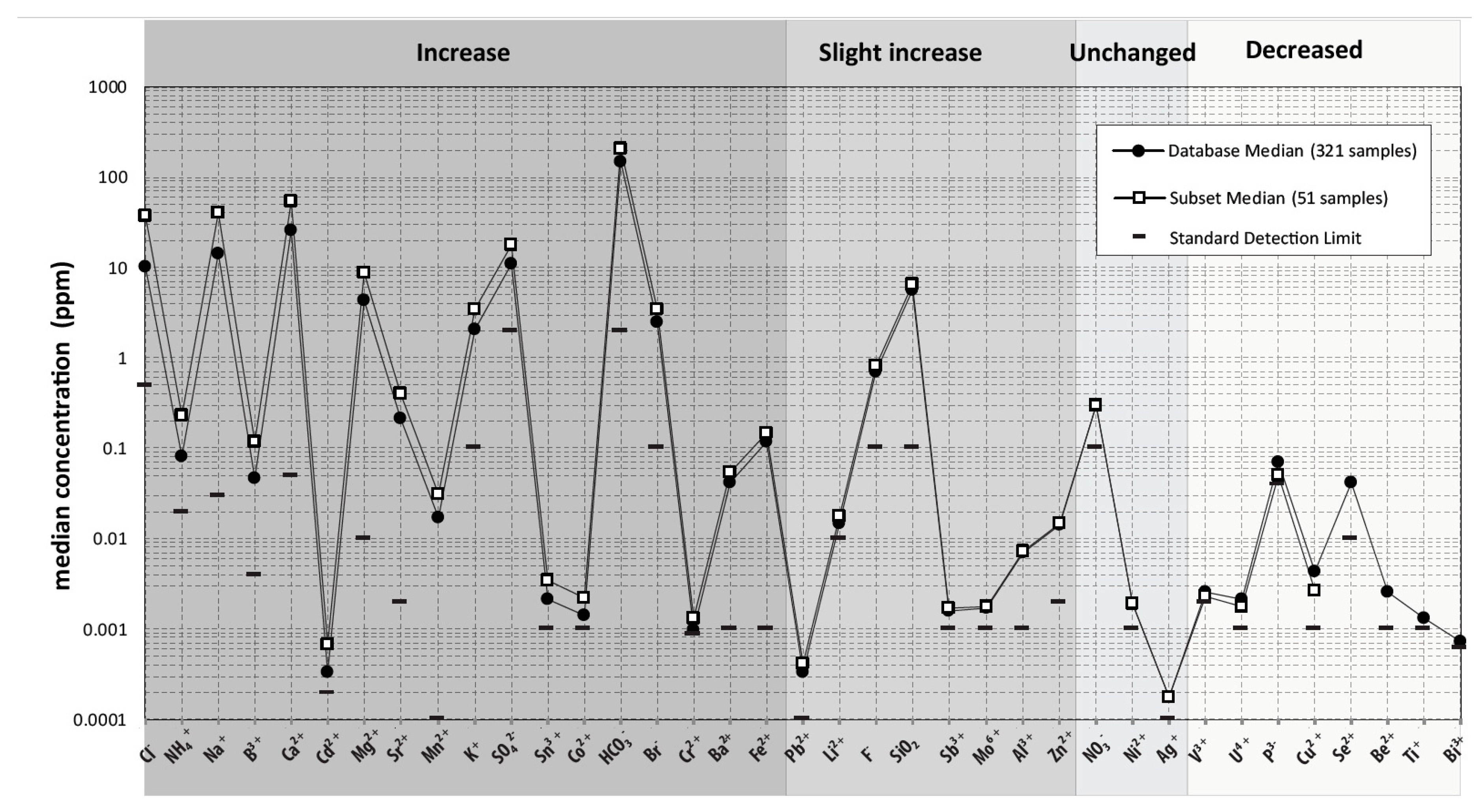
5.2. Chemical Characteristics of the Subset versus the Regional-Scale Database

Figure 5 shows the comparison between the detection ratios for the regional-scale database (N = 321 samples) and the subset (N = 51 samples). On the x-axis, the ionic species are sorted in descending order of detection ratio for the regional-scale database. For the subset, four new chemical elements have now risen above 75% of data > DL: fluoride, ammonium, iron, and molybdenum. A total of 18 chemicals could be justifiably included in the statistical multivariate treatment (valid data exceeding 75%). Only the detection ratio for aluminum and chromium has decreased slightly.

To evaluate the effect of the dataset reduction, the ionic content difference of the regional-scale database is compared to the subset of samples. Figure 6 shows the comparison between the median concentration in ppm for each chemical element of the database and the subset on a log scale (y-axis). Chemical elements (x-axis) are sorted in descending order of differences between median concentrations (∆ median concentration - m.c. - expressed in ppm) for the 321 sample database and the 51 sample subset. Variations in the medians of the two datasets calculated in percentages are presented in the supplementary material (Supplementary Materials S2).

By reducing the regional-scale database, the ionic content of the 51 sample subset increased, although the median concentration (m.c.) of some chemical elements remained unchanged or decreased. Chemical elements with decreasing content are vanadium (88% of the m.c. of the 321 sample database), uranium (86% of the m.c. of the 321 sample database), phosphate (71% of the m.c. of the 321 sample database), and copper (63% of the m.c. of the 321 sample database). Selenium, beryllium, titanium, and bismuth are all <DL in the 51 sample subset. For silver, nitrate, and nickel, the m.c. for the 51 sample subset is equal to the m.c. for the 321 sample database. The most significant increase is for chloride (370% of the m.c. of the 321 sample database) and ammonium (288% of the m.c. of the 321 sample database). The correlation matrices for the subset and the database (Supplementary Materials S1 and S3) showed that ammonium was highly correlated with the major elements (K⁺, HCO₃⁻, Mg²⁺, Na⁺, Ca²⁺, Cl⁻,and SO₄²⁻), as well as some minor elements (Ba²⁺, Sr²⁺, and B³⁺) and some trace elements (Li²⁺, Br⁻ and Pb²⁺). The possible origin of dissolved ammonium is discussed based on factorial analysis results in Section 6.

Compared to the original 321 sample dataset, the 51 sample subset contains concentrated samples for major (cation and anion), minor, and some trace metallic elements and is depleted for some ultra-trace elements (selenium, beryllium, titanium, and bismuth). The overall enrichment of the subset suggests that groundwater chemistry of the subset is more mature in terms of water/rock interactions. Thus, the subset is suitable for studying the link between groundwater mineralization processes (i.e., salinization) and the presence of specific dissolved ions.

5.3. Results Comparison between Subset and Regional-Scale Database

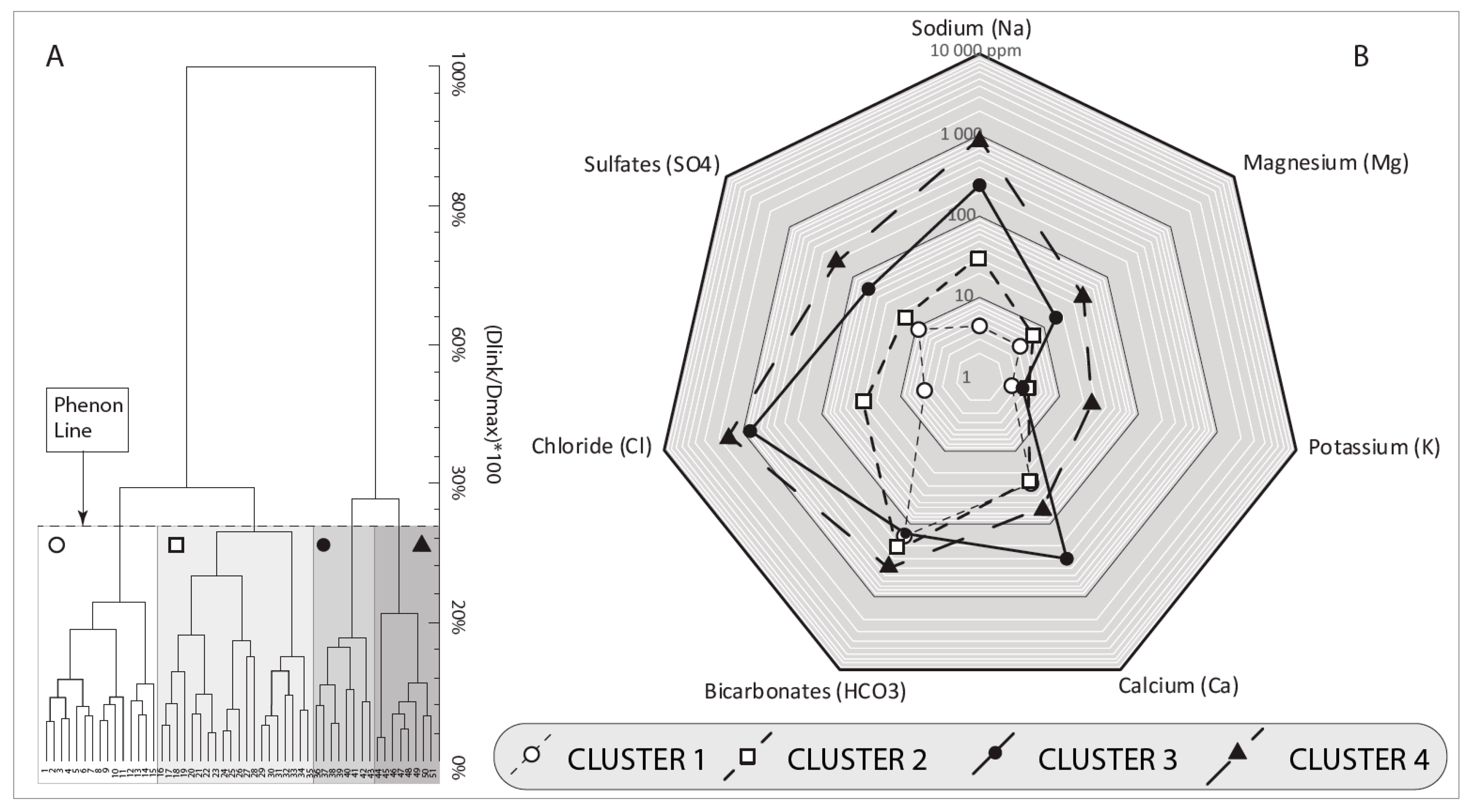
5.3.1. Hierarchical Cluster Analysis Results

In hierarchical Cluster analysis (HCA), the number of Clusters is determined by the position of the phenon line that cuts across the resulting dendrogram (Figure 7A). In our HCA, the distance linkage (Dlink) of the samples is expressed as a percentage of the maximum distance (Dmax) between the most dissimilar samples ([Dlink/Dmax] × 100). At this scale, 100% linkage (Dlink = Dmax) would indicate that all samples are grouped into a single Cluster that corresponds to the 51-sample subset. For this study, four Clusters (Dlink < 30% of Dmax) were selected (Figure 7A). Major cation and anion concentrations for the four Clusters were projected on a log-scale spider diagram in ppm (Figure 7B).

Table 5. Water type, aquifer type, and chemical content (median) of the 4 Clusters obtained by hierarchical Cluster analysis.

	Cluster 1 (N = 15)	Cluster 2 (N=20)	Cluster 3 (N = 8)	Cluster 4 (N = 8)
Water Type	Na-Cl (0)/Ca-Cl (0)	Na-Cl (2)/Ca-Cl (1)	Na-Cl(3)/Ca-Cl(5)	Na-Cl (8)/Ca-Cl (0)
	Na-HCO3 (0)/Ca-HCO3 (15)	Na-HCO3 (6)/Ca-HCO3 (11)	Na-HCO3 (0)/Ca-HCO3 (0)	Na-HCO3 (0)/Ca-HCO3 (0)
Aquifer Type	Rock (6)/Granular (9)	Rock (12)/Granular (8)	Rock (7)/Granular (1)	Rock (1)/Granular (7)
Hydrogeological Context *	UnC (10)/C (0)/UnK (6)	UnC (6)/C (7)/UnK (7)	UnC (5)/C (0)/UnK (3)	UnC (1)/C (6)/UnK (1)
	Median	Median	Median	Median
TDS (mg/L)	229.6	402.4	1733.1	3142.6
Temperature (Celcius) **	7.68	7.58	7.77	7.69
Redox potential (mV) **	100.5	84.05	−24.45	−48.25
pH **	7.49	7.57	7.80	7.46
Dissolved oxygen (mg/l) **	2.65	0.00	0.00	0.00
Sodium	4.40	32.50	240.00	905.00
Magnesium	4.30	7.00	16.00	42.50
Potassium	2.50	4.05	3.40	26.00
Calcium	28.00	25.50	300.00	59.00
Bicarbonates	146.40	231.80	134.20	403.82
Chloride	5.10	29.50	815.00	1500.00
Sulfates	9.40	15.50	58.00	190.00
Barium	0.026	0.058	0.190	0.048
Boron	0.010	0.050	0.235	0.475
Strontium	0.180	0.375	12.900	1.650
Silicium	5.700	6.600	5.100	8.950
Manganese	0.014	0.014	0.079	0.061
Fluoride	0.200	0.750	1.300	1.450
Aluminium	0.007	0.008	0.005	0.006
Bromide	<DL	<DL	11.500	5.553
Iron	0.071	0.105	0.140	0.190
Lithium	<DL	<DL	0.076	0.019
Zinc	0.0240	0.0110	0.005	0.015
Lead	<DL	<DL	<DL	<DL
Ammonium	0.040	0.195	0.460	1.282
Copper	0.006	0.001	<<DL	<DL
Molybdenium	0.001	0.002	0.0048	0.002
Nickel	<DL	0.001	<<DL	<DL
Silver	<DL	0.0001	<DL	<DL
Uranium	<DL	<DL	<DL	0.001
Chromium	<DL	<DL	<DL	<DL
Nitrate	0.300	0.060	<DL	<DL
Sulfide	NA	NA	<DL	<DL
Cobalt	<DL	<DL	<DL	<DL
Inorganic phosphorus	<DL	<DL	<DL	0.042
Vanadium	<DL	<DL	<DL	<DL
Antimony	<DL	<DL	<DL	<DL
Cadmium	<DL	<DL	<DL	<DL
Selenium	<DL	<DL	<DL	<DL
Tin	<DL	<DL	<DL	<DL
Titanium	<DL	<DL	<DL	<DL
Beryllium	<DL	<DL	<DL	<DL
Bismuth	<DL	<DL	<DL	<DL

* Unconfined (UnC); Confined (C); Unknown (UnK); ** multiparameter probe (in situ); TDS is calculated using the software Aquachem v.5.0; For major, minor and trace elements, data are given in mg/L; Under Detection Limit (<DL); Non Applicable (NA); Parameters presented in bold characters have been selected for multivariate treatment.

shows the median concentrations for the physical and analytical parameters, as well as the water type, aquifer type, and hydrogeological context of the Clusters.

Clusters 1 and 2 are composed largely of bicarbonate waters (32/35 samples), while Clusters 3 and 4 are composed of groundwater dominated by chloride anion (16/16, Table 5). All samples in Cluster 1 are composed of groundwater of the Ca-HCO₃ type, while the samples in Cluster 2 are composed mainly of groundwater of the Ca-HCO₃ (11/20) and Na-HCO₃ type (6/20), with a limited number of groundwater samples of the Na-Cl type (2/20).

Clusters 3 and 4 are dominated by chloride, sulfate, and sodium. Samples from Cluster 3 were collected mostly from fractured rock aquifers (7/8 samples). The very large proportion of Cluster 4 corresponds to groundwater samples collected in granular aquifers (7/8 samples), mostly confined (6/8 samples). The samples from Cluster 1 come mainly from unconfined aquifers, and Cluster 2 samples were collected in equal proportions in confined aquifers or in unconfined aquifers. Cluster 3 is dominated by Ca-Cl (5/8) samples and contains some Na-Cl (3/8) samples. Cluster 4 consists exclusively of groundwater of the Na-Cl type.

The results obtained using HCA are like those described in [5] for the regional-scale database (321 samples). Both studies allow for the identification of a Cluster dominated by fractured rock groundwater samples, two Clusters of saline groundwater samples, and at least a Cluster dominated by groundwater samples of the bicarbonate type. Thus, the reduction of the original dataset into a subset does not modify the Clustering obtained with HCA processing.

Some distinctions between the two studies are, however, of interest. By positioning the phenon line to obtain four Clusters, the Clusters obtained with the subset of data have a lower percentage of resemblance (27% against 52% in [5]) to the regional-scale database. This observation suggests that the differences between the groups are better defined using the data reduction approach of this study, having the effect of reducing the general geochemical similarities between the samples. This result can be understood as the reduction of background noise, or the identification within the regional-scale database of more representative samples of hydrogeochemical endmembers (early stage or advanced stage of evolution) of the regional hydrogeochemical poles (RHPs). The background noise would then correspond to all types of mixing phenomena that lead to a certain homogenization of the general hydrogeochemistry.

Another difference between the results of the two studies is in the Clustering of bicarbonate-type groundwater samples. Whereas [5] identify only one Cluster of bicarbonated groundwater (the most populated, 274 samples out of 321), the HCA applied to the subset of data allows for the definition of two Clusters (Cluster 1 and Cluster 2). Reducing the dataset, therefore, brought out two chemical signatures specific to bicarbonate groundwaters in the study area, Cluster 1 dominated by calcium and Cluster 2 dominated by sodium. The transformation of calcium hydrofacies into sodium hydrofacies is interpreted as one of the first stages in the evolution of groundwater, particularly in crystalline fractured aquifers [24]. Clusters 1 and 2 (bicarbonate groundwater) both have a similar proportion of groundwater samples from crystalline rock and granular deposits (Table 5). In the SLSJ region, the evolution of calcium bicarbonate water to sodium bicarbonate water is also effective in the groundwater contained in confined granular deposits, where marine clay acts as a cation exchanger by releasing sodium in exchange for calcium [5,25]. Clusters 1 and 2, respectively, represent two successive stages in the evolution of recharge water: on the one hand, in fractured rock aquifers, and on the other hand, in granular aquifers confined by marine clays.

The use of HCA with the reduced dataset also allowed for the grouping of samples of brackish water taken from confined granular aquifers (Cluster 4; Table 5). In [5], no distinction was possible between brackish groundwater from fractured rock aquifers and from confined granular aquifers.

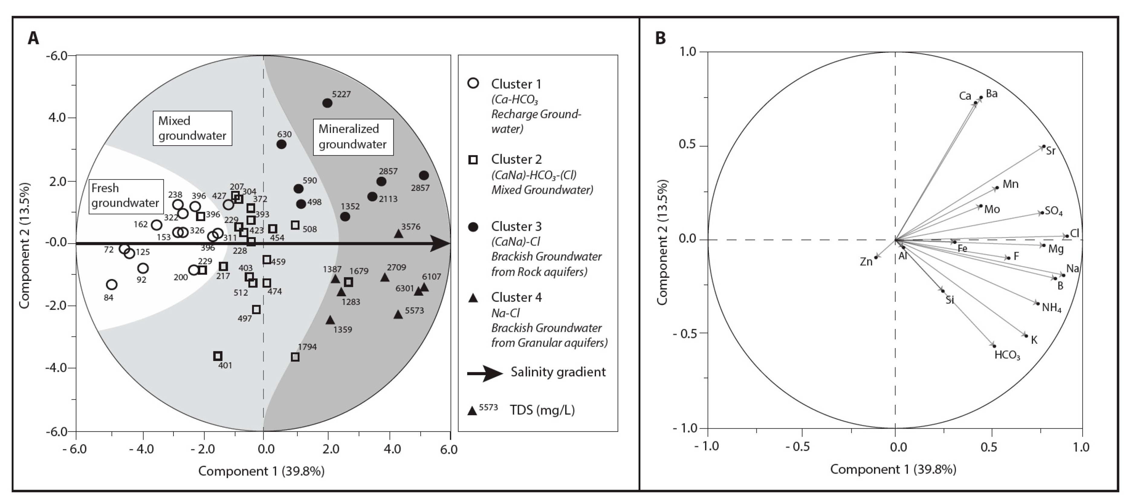
5.3.2. Principal Component Analysis Results

Samples, labeled with their Cluster number as defined in Figure 7A, are plotted on the PCA correspondence circle (Figure 8). The horizontal axis of the correspondence circle corresponds to the first principal component (Component 1; 39.8% of the total variance of the dataset), and the vertical axis corresponds to the second principal component (Component 2; 13.5% of the total variance of the dataset). In Figure 8A, TDS is indicated for each sample. Increasing TDS from left to right along component 1 indicates that component 1 corresponds to a salinity gradient. Chemical element loadings for components 1 and 2 are plotted in the correspondence circle in Figure 8B. Component 2 scores are positive for Cluster 3 samples. Chemical elements with positive scores for component 2 are Ca²⁺, Ba²⁺, Sr²⁺, Mn²⁺, Mo⁶⁺, and SO₄². Component 2 scores are negative for Cluster 4 samples. Chemical elements with negative scores for component 2 are Mg²⁺, F⁻, Na⁺, B³⁺, NH₄⁺, SiO₂⁺, K⁺, and HCO₃⁻.

The results obtained with the PCA also show a good correspondence with the study of [5] performed on the regional dataset. In both studies, the chemical elements calcium, barium, strontium, manganese and sulfate are associated with Cluster 3 (water-rock interactions), and magnesium, sodium, boron, silica, potassium, and bicarbonate are associated with Cluster 4 (water-clay interaction type). Both studies suggest that an increase of the salinity enhances the fingerprint of the hydrogeological context (nature of the aquifer and hydraulic conditions) on the major ions of groundwater chemistry.

However, the regional-scale database reduction approach described in this paper allows for new insights into the presence of certain undesirable ions, such as fluorides. Fluorides are associated with Cluster 4, suggesting that some of the fluorides come from environments dominated by water-clay interactions, as suggested by [5]. The water-clay interactions are characterized by a combination of processes: ion exchange, salt leaching of the regional aquitard made of marine clays, or both. It would be relevant to investigate how these mechanisms could lead to an increase of fluorides in groundwater. Clearly, the marine clay found in the SLSJ region is suspected of releasing fluoride into the groundwater, where confining conditions of the aquifers prevail. This assumption is also valuable for the clays originating from the last marine invasion (approximately 10,000 years ago) elsewhere in Quebec Province.

The PCA results also give molybdenum with Cluster 3 (water-rock interactions) and ammonium in association with Cluster 4 (water-clay interactions). Again, these results raise questions about the possible links between these elements and their hydrogeochemical context.

5.3.3. New Graphical Fields and Interpretations Improvement

Walter et.al. [5] discussed the evolution of groundwater using binary graphs and the Piper diagram. Using the same graphs, the interpretation of the hydrogeochemical evolution remains the same but appears in a much more revealing way. A good example is given in Figure 9, the log-log [Ca²⁺ vs. Na⁺] plot. This figure is similar to the figure presented in [5], with the difference that the Clusters (1 to 4) in Figure 9 correspond to the Clusters identified with the reduced dataset method developed in this study.

The alignment of the Cluster samples observable in Figure 9 indicates a gradual progression of the bicarbonate-type endmembers (Clusters 1 and 2) toward the brackish endmembers (Clusters 3 and 4). Pathways for bicarbonate-type groundwater evolving to brackish groundwater can be proposed by linking Clusters 1 (recharge waters) to Clusters 3 and 4 (brackish groundwater) going through Cluster 2 samples (recharge to intermediate groundwater). Calcium and sodium content evolution pathways presented in Figure 9 define new fields that can be compared to the dilution line of seawater but in terms of water/rock interactions (Pathway 2; Figure 9) and water/clay interactions (Pathway 2; Figure 9).

The mineralization of groundwater usually corresponds to a process of salinization, since the increase of the residence time of the water in the aquifer enhances the dissolution of salt minerals contained in the solid fraction of the porous medium. This causes the groundwater to evolve from a dilute calcium bicarbonate type in recharge areas toward a more concentrated sodium chloride or calcium chloride type along the flow path. The method proposed in this article makes it possible to statistically identify, in a regional database, a series of samples representing the successive stages of the natural evolution of groundwater. These samples were taken from different locations in the study area, but their chemistry corresponds to the possible evolution of groundwater along a regional flow line according to [19] (salinization path 1), or from interaction with marine clay or mixing with seawater (salinization path 2).

Other samples of the regional-scale database previously discarded to form the subset also follow the pathways (Figure 9). As a first approximation, based on their calcium and sodium content, these samples can then be designated as belonging to one of the three main hydrogeochemical contexts: recharge-type groundwater (blue shape in background), groundwater of the water-rock interactions type (red shape in background), and groundwater of the water-clay interactions type (green shape in background). This result gives a first approximation of the hydrogeochemical context of groundwater using the calcium and sodium content of groundwater.

Groundwater chemical evolution can also be discussed by considering major cations and major anions of groundwater using a Piper plot. In Figure 10, the samples are marked with symbols representing the first approximation of the hydrogeochemical context (recharge-type groundwater, water-rock-type interactions, and water-clay-type interactions) interpreted using a Ca²⁺ vs. Na⁺ binary plot (Figure 9). Seawater is also shown on the Piper diagram (Figure 10). Clusters presented in Figure 9 are those identified using the reduced set of data.

The proposed method leads to the improvement of the interpretations of the Piper diagram. Based on the reduced dataset, new graphical fields of the Piper diagram are defined for the study area (Figure 10B). Groundwaters that evolved in the context of water-rock interactions are found in the upper part of the lozenge surface, and in the lower part, it is the samples in the context of water-clay interactions that dominate. The samples from Cluster 2 mark a very clear intermediate position between the samples from Cluster 3 and Cluster 4. At the origin of this demarcation, it is the transformation of the calcium facies toward a sodium facies. This intermediate position makes the transition between the signature of recharge-type waters and the brackish groundwater. Based on the interpretations of the hydrogeochemical context from Figure 9, the losangic surface can be split into two parts, by joining the recharge-type pole and the seawater pole (Figure 10B).

A mixing zone is interpreted at the boundary between the two parts of the lozenge surface. The hydrogeochemical context has little impact on the magnesium and sulfate content of groundwater, although magnesium has a slight affinity for water-rock interactions and sulfates preferentially characterize recharge-type waters and water-rock interactions locally.

5.4. Factor Analysis

Normalized Varimax rotation was applied to the factors [1,3,23]. The Kaiser criterion [23,24,25,26] helps to determine the number of factors to be retained; only those components with Kaiser criterion greater than 1 were retained. Factors were calculated on the symmetrical covariance matrix computed for 16 variables (K⁺, HCO₃⁻, Mg²⁺, SiO₂, NH₄⁺, F⁻, B³⁺, Mo⁶⁺, Na⁺, Ca²⁺, Ba²⁺, Sr²⁺, SO₄²⁻, Fe²⁺, and Mn²⁺). Chloride has been consciously discarded from the factorial analysis after observation of the correlation matrix (Supplementary Materials S1 and S3), as Cl⁻ was highly correlated with all the other major elements and some trace elements and would induce a redundancy. The correlation matrix for the 51-sample subset also revealed that aluminum and zinc had no significant correlation with other chemical elements. To prevent noise introduction in the multivariate statistical treatment, aluminum and zinc have been discarded as well.

The first four factors present loadings (i.e., explained variance;

Table 6. Factor analysis loadings and explained variance after applying a Varimax rotation.

Parameter	Factor 1	Factor 2	Factor 3	Factor 4
Potassium	0.87	0.21	−0.03	0.24
Bicarbonates	0.71	0.24	−0.22	0.22
Magnesium	0.70	0.22	0.45	0.15
Silicium	0.67	−0.34	0.08	0.00
Ammonium	0.64	0.49	0.05	0.28
Fluoride	0.16	0.90	0.07	−0.12
Boron	0.50	0.78	0.15	0.10
Molybdenum	−0.12	0.77	0.20	0.04
Sodium	0.60	0.70	0.23	0.03
Calcium	0.02	−0.05	0.93	0.20
Barium	−0.11	0.15	0.83	0.15
Strontium	0.21	0.47	0.79	0.09
Sulfates	0.61	0.22	0.62	−0.03
Iron	0.26	−0.14	0.08	0.82
Manganese	0.14	0.16	0.40	0.80
Explained variance	3.77	3.33	3.10	1.63
Explained variance (%)	25.1	22.2	20.6	10.8
Cumulative % of variance	25.1	47.3	68.0	78.8

) greater than 1 and account for 78.8% of the total variance of the subset. The first factor (25.1% of the total variance) is characterized by high loadings for K⁺, HCO₃⁻, Mg²⁺, SiO₂, NH₄⁺, and SO₄²⁻. Loadings for F⁻, B³⁺, Mo⁶⁺, and Na⁺ explain the second factor (22.2% of the total variance). Loadings for the third factor (20.6% of the total variance of the subset) are dominated by Ca²⁺, Ba²⁺, Sr²⁺, and SO₄²⁻. Finally, the fourth factor (10.8% of the total variance of the subset) is strongly influenced by Fe²⁺ and Mn²⁺.

6. Discussion

The statistical treatments generated four clusters of water compositions in link with aquifer types and water evolution. However, numerous processes and sources can account in part for critical health elements. In particular, (1) the evolution of the recharge water, (2) the fingerprinting of the Laflamme water sea, (3) the Precambrian basement contribution, and (4) the specific sources of fluorides are addressed below linked with statistical grouping (cluster and factor).

6.1. Evolution of Recharge Groundwater (Clusters 1 and 2; Factor 4)

Clusters 1 and 2 belong to a recharge-type groundwater. The fourth factor explains only 10.8% of the total variance of the data set, and thus characterizes only a few samples among the 51 sample subset. In Figure 11c,e,f, sample scores for the fourth factor are projected onto the y-axis. This factor presents high loadings for Fe²⁺ and Mn²⁺ (Table 5). These are redox-sensitive species [27,28], and thus, their concentrations in groundwater are primarily influenced by the amount of available dissolved oxygen [29]. In the presence of dissolved oxygen, principally near surface environments, iron and manganese will be solubilized by oxidizing and acidic conditions that tend to increase the Fe²⁺ and Mn²⁺ content in groundwater. This finding may explain why Factor 4 predominantly influences (CaNa)-HCO₃ groundwater (Clusters 1 and 2; Figure 11c,e,f).

Negative values for the fourth factor can be interpreted as a lack of correlation between the two chemical elements. Based on the Eh-pH diagram (Supplementary Materials S4), the range of stability for dissolved Fe²⁺ differs from the range of stability of Mn²⁺. Depending on the Eh-pH conditions, Fe²⁺ and Mn²⁺ may not coexist in the soluble form. For instance, iron precipitates as hydroxide while manganese remains dissolved, possibly at the origin of the negative values obtained for the fourth factor in Figure 11c,e,f.

Negative values are recorded in the recharge type of groundwater (predominantly Cluster 2) that follows the freshwater influx vector interpreted at the bottom left quarter in Figure 11c,e,f, suggesting that early in the groundwater evolution, iron was mobilized by the physical environment of the aquifer, while manganese stayed dissolved in groundwater.

6.2. Fingerprint of the Laflamme Seawater (Cluster 4; Factor 1)

Positive scores for the first factor are recorded for samples from Cluster 4 (Figure 11a–c, highlighting the influence of the first factor on Cluster 4 samples. The first factor is characterized by high loadings of K⁺, HCO₃⁻, SiO₂, NH₄⁺, SO₄²⁻, and Mg²⁺ (Table 6).

Wang et al. [30] argued recently that dissolved NH₄⁺ found in groundwater originates from overlying marine clay aquitards. The aquitard plays a role of a strong anaerobic environment favorable for mineralization of sedimentary organic matter. Degradation of organic matter would produce CO₂ gas and favor the formation of HCO₃⁻. For PCA results, NH₄⁺ preferentially characterizes groundwater in Cluster 4 and is correlated to HCO₃⁻ in this cluster. Sulfate reduction also produces CO₂. If SO₄²⁻ reduction enhances the production of HCO₃⁻ by the dissociation of water molecules in the presence of CO₂, this reaction is accompanied by the production of aqueous HS⁻ gas [31]. The general reaction is given as follows:

SO₄²⁻ + 9H⁺ + 8e⁻ → HS⁻ + 4H₂O

(1)

The regional chemical characterization of groundwater showed that sulfide gas was preferentially detected in granular confined environments, where handmade piezometers were installed for a private water supply [8]. For Cluster 4, SO₄²⁻ might have a marine origin, i.e., seawater trapped in the marine aquitard. Sulfide isotopes would help to test this hypothesis.

Based on mineralogical analyses performed on deep marine deposits from some areas in the SLSJ region [32], the chemical breakdown of silicate minerals, for instance, microcline, was at the origin of SiO₂ and K⁺ in groundwater (Equation (2); [5]). This assumption is reinforced by factorial analysis (FA) results here.

3KAlSi₃O₈ + 2H⁺ → 2K⁺ + 6SiO₂ + KAI₃Si₃O₁₀(OH)₂
(microcline)   (illite)

(2)

Variations in the chemical elements for Factor 1 (K⁺, HCO₃⁻, SiO₂, NH₄⁺, and SO₄²⁻) are believed to characterize groundwater from a confined environment due to the presence of the regional marine aquitard (water-clay interactions; [5]). The first factor characterizes the tendency of groundwater to evolve toward an end-member with a composition similar to that of the present seawater (i.e., Na-Cl-rich in composition).

6.3. Fingerprinting of the Precambrian Shield Brines (Cluster 3; Factor 3)

Chemical data for brines found at depth in the Canadian Shield were compiled from the existing literature to compare the geochemical trend of the samples from this study. A total of 137 chemical analyses from five studies were included: [33], 33 samples; [34], 24 samples; [35], 36 samples; [36], 35 samples; and [24], 17 samples. The compiled data are presented as Supplementary Materials S5.

In Figure 11b,d,f, samples from Cluster 3 are predominantly influenced by the third factor with loadings dominated by Ca²⁺, Ba²⁺, Sr²⁺, and SO₄²⁻ (Table 5). Log-log plots of Ca²⁺, Ba²⁺, Sr²⁺, and SO₄²⁻ versus Cl⁻ concentrations (Figure 12A–D) for the subset of samples in this study were coupled with the data from other Canadian Shield brines.

Frape et al. [36] determined that the geochemistry of Ca²⁺ plays a major role in controlling the chemistry of mineralized groundwater in the crystalline bedrock of the Canadian Shield. Frape et al. [36] described very old stagnant groundwater that may have undergone prolonged chemical alteration since its original emplacement. The similar Ca²⁺/Cl⁻ trend for the Cluster 3 and the Precambrian Shield brines (PSB) (Figure 12A) suggests a common origin for Ca²⁺ and Cl⁻.

In Figure 12A,D, Ca²⁺ and Sr²⁺ concentrations for Clusters 3 and 4 show similar trends, suggesting a common origin for Sr²⁺ and Ca²⁺ in Cluster 3. For Sr²⁺, as well as Ba²⁺, it is commonly found incorporated as a trace element in the crystalline structure of feldspar plagioclase minerals [37,38]. In Figure 12B, the trend for Ba²⁺ is different from the trend for Sr²⁺ and Ca²⁺. Edmunds and Smedley [39] showed that barite solubility controls Ba²⁺ concentration and that Ba²⁺ quickly reaches saturation or supersaturation in recharge groundwater. In Figure 12B, Ba²⁺ concentrations for Clusters 1 and 2 reach levels similar to the concentrations for Clusters 3 and 4, suggesting that maximal Ba²⁺ concentrations are attained in recharge-type groundwater.

Unlike Ba²⁺, Sr²⁺ is not limited in terms of solubility [39]. Some of the Sr²⁺ may be added by the dissolution of anhydrite or gypsum. However, SO₄²⁻ vs. Cl⁻ (Figure 12C) shows a trend different from Sr²⁺ vs. Cl⁻ (Figure 8d), refuting this possibility. According to [24], most of the added Cl⁻ and some SO₄²⁻ in groundwater collected in selected granitic, gabbroic, and gneissic plutons in the Canadian Shield are derived from the rock matrix. Ions are present either as soluble salts in fluid inclusions and along grain surfaces [40] or as structurally bound elements in micas and amphiboles [41]. Sulfate may then be more derived from the oxidation of sulfide minerals in the rock matrix rather than due to the presence of gypsum-infilling minerals in the fractures.

For Cluster 3 samples, the strong relationship of Ca²⁺ and Sr²⁺ versus Cl⁻ concentrations, the Ba²⁺ content for recharge groundwater, and the similar trends with the Precambrian Shield brines (PSB), all suggest that Cluster 3 corresponds to some diluted endmembers with a composition such as the PSB compiled in this study. Thus, Cluster 3 belongs to a PSB-type of groundwater. A ratio Ca²⁺/Sr²⁺ ≈ 40 is proposed here to identify the PSB groundwater type.

6.4. Sources of Dissolved Fluoride in Groundwater (Factor 2)

The second factor requires investigation as it may provide clues to the origin of dissolved fluoride in groundwater. Factor 2 is characterized by high loadings of F⁻, B³⁺, Mo⁶⁺, and Na⁺ (Table 6).

In the study area, F⁻ concentrations of 20% of the sampled wells [9] exceed both the Canadian drinking water quality guidelines [14] and the WHO standards [4]. Sample scores for Factor 2 are projected on the x-axis in Figure 11d,e and on the y-axis in Figure 11a. Factor 2 influences groundwater from Clusters 2, 3, and 4. The source of F⁻ is ambiguous. Since more than one group is influenced by the second factor. The covariations of the chemical elements that compose Factor 2 suggest multiple processes of interaction between groundwater and the solid matrix of aquifers or aquitards for explaining the origin of fluoride in groundwater. Numerous sources and processes have been proposed and are detailed below.

Boron (B³⁺) and Mo⁶⁺ are found incorporated into the crystalline structure of tourmaline and molybdenite, two very common minerals in pegmatite of Grenville Province (Carignan and Gariépy, 1992) that constitute some of the Precambrian rock of the study area. Despite the low solubility of these minerals, the long-term interaction between groundwater and granitic rocks could account for their source, hence explaining the covariations of B³⁺, Mo⁶⁺, and F⁻. Recent studies showed that micas in granitic rocks are the main source of dissolved fluoride in groundwater [43,44,45]. Experiments with regional rocks should be performed to test if this hypothesis is possible for the study area.

Boron has been described in the SLSJ region where shales are present [46]. Mo⁶⁺ is also frequently found in fossil fuels [38]. Occurrences of gas and oil in shales and limestones have been identified in the study area [8]. The combination of B³⁺ and Mo⁶⁺ could indicate that F⁻ originates from the groundwater interaction with organic matter-rich sedimentary rocks present in the region. Investigations on a local scale would help to test this hypothesis.

Walter [45] explained that the geochemical behavior and concentration of fluorine in groundwater are controlled by the existence of Ca-bearing minerals and by the fluorite precipitation as a function of the absolute concentration of Ca²⁺ ions in water. In the study region, Walter et al. [5] suggested that the Ca²⁺_water-Na⁺_mineral ion exchange processes may lead to a decrease in the groundwater Ca²⁺ content. As fluorite (CaF₂) equilibrium controls F⁻ and Ca²⁺ concentrations [47], it is expected that the removal of Ca²⁺ from the water in exchange for Na⁺ will increase the fluoride (F⁻) concentration in presence of fluorite. A slight increase in F⁻ is observed in Table 5 between Clusters 1 and 2 (Recharge-like), and would suggest the presence of fluorite in the system.

The Ca²⁺_water-Na⁺_mineral ion exchange processes also support the linear correlation of Na⁺ and F⁻ in Factor 2. Ion exchange is believed to occur early in the evolution of groundwater in bedrock aquifers [24] but also particularly characterizes groundwater from confined aquifers [5].

Overall, dissolved F⁻ can be generated either from the interaction of groundwater with marine clay or from the interaction of groundwater with bedrock aquifers in the early stage of evolution of recharge type of groundwater, also suggesting that a great environment for enhancing groundwater fluoride content would be the crystalline bedrock aquifers confined by the marine clay aquitard.

7. Conclusions

This study proposed a new approach for diminishing the negative impact of censored values in large databases for multivariable treatments to better constrain chemical evolution and sources of ions for groundwater. The approach involves first data grouping accounting for regional hydrogeochemical poles (RHP). Second, key chemical elements are identified in each of the groups by considering the detection ratio, which is obtained by comparing to the analytical detection limit as % NDetected = [NDetected/NDatabase] × 100. Selected key elements have high detection ratios in a specific RHP.

The groups of the subset were treated by a combination of hierarchical Cluster analysis (HCA), principal component analysis (PCA), binary plot investigations, and Piper diagrams to decipher geochemical trends and processes. The results obtained with the subset are consistent with those of [5] obtained with a regional-scale database. Furthermore, the subset allowed for factor analysis (FA), bringing new insights into the chemical evolution of groundwater through the salinization process. Four factors accounted for 78.8% of the total variance.

Factor 1, with high loadings for K⁺, HCO₃⁻, Mg²⁺, SiO₂, NH₄⁺, and SO₄²⁻, characterizes groundwater in contact with the regional clay aquitard. The chemical transformation of microcline into illite and CO₂ production control the chemistry of groundwater in confined aquifers. Factor 2 has loadings for F⁻, B³⁺, Mo⁶⁺, and Na⁺. Dissolved F⁻ can be generated either from the interaction of groundwater with marine clay or from bedrock aquifers (crystalline or sedimentary aquifers).

Part of the discussion of this article focuses on hypothetical regional sources of fluoride by studying the FA results obtained using the subset of data. The results partly explains why the groundwater chemical background of the region has relatively high levels in fluoride, resulting in frequent excess of drinking water standards. Subsequent studies may now attempt to test the proposed processes experimentally (batch experiments) and numerically (speciation and geochemical modeling).

The third factor is dominated by Ca²⁺, Ba²⁺, Sr²⁺, and to a lesser extent, SO₄²⁻. The third factor characterizes samples corresponding to a diluted endmember of the Precambrian Shield brines (PSBs). The diluted endmember of the PSBs in this study have been compared with PSBs compiled from the literature on log-log plots of Ca²⁺, Ba²⁺, SO₄²⁻, and Sr²⁺ versus Cl⁻ concentrations. A mass ratio Ca²⁺/Sr²⁺ ≈ 40 is proposed to identify groundwater that experienced geochemical processes leading to a composition, such as the Canadian Shield brines. Factor 4 is strongly influenced by Fe²⁺ and Mn²⁺ and characterizes the recharge-like type of groundwater (Cluster 1 and 2), where in the first stage of groundwater evolution, iron precipitate while manganese remains dissolved.

In this study, samples from the subset belong to the same flow path from a statistical point of view, not from a geographical point of view. Others samples from the database can then be compared with the samples of the subset and discussed according to their stage of evolution. Our results demonstrated that the dataset reduction could be a better approach for the study of water-rock interaction mechanisms based on truncated distribution. Other selection methods must be tested. Rather than detection limits, quartiles or water quality standards could be used as criteria for deciphering patterns in large-scale databases.

References

1. Alvin, C.R. Methods of Multivariate Analysis; Wiley Interscience: Hoboken, NJ, USA, 2002. [Google Scholar]
2. Farnham, I.M.; Johannesson, K.H.; Singh, A.K.; Hodge, V.F.; Stetzenbach, K.J. Factor analytical approaches for evaluating groundwater trace element chemistry data. Anal. Chim. Acta 2003, 490, 123–138. [Google Scholar] [CrossRef]
3. Brown, C.E. Applied Multivariate Statistics in Geohydrology and Related Sciences; Springer: Berlin, Germany, 1998. [Google Scholar]
4. World Health Organization. Guidelines for Drinking-Water Quality: Recommendations, (Vol. 1); World Health Organization: Geneva, Switzerland, 2004. [Google Scholar]
5. Walter, J.; Chesnaux, R.; Cloutier, V.; Gaboury, D. The influence of water/rock—Water/clay interactions and mixing in the salinization processes of groundwater. J. Hydrol. Reg. Stud. 2017, 13, 168–188. [Google Scholar] [CrossRef]
6. Laurin, A.F.; Sharma, K.N.M. Mistassini, Peribonka, Saguenay Rivers Area: Grenville 1965–1967; Ministère des Richesses Naturelles, Direction générale des mines, Geological Exploration Service: Québec, QC, Canada, 1975. [Google Scholar]
7. Desbiens, S.; Lespérance, P.J. Stratigraphy of the Ordovician of the Lac Saint-Jean and Chicoutimi outliers, Quebec. Can. J. Earth Sci. 1989, 26, 1185–1202. [Google Scholar] [CrossRef]
8. CERM-PACES. Résultats du Programme D’acquisition de Connaissances sur les Eaux Souterraines du Saguenay-Lac-Saint-Jean, Centre D’études sur les Ressources Minérales; Université du Québec à Chicoutimi: Saguenay, QC, Canada, 2013. [Google Scholar]
9. Walter, J.; Rouleau, A.; Chesnaux, R.; Lambert, M.; Daigneault, R. Characterization of general and singular features of major aquifer systems in the Saguenay-Lac-Saint-Jean region. Can. Water Resour. J./Revue Can. Ressour. Hydr. 2018, 43, 75–91. [Google Scholar] [CrossRef]
10. Dionne, J.; Laverdière, C. Sites fossilifères du golfe de Laflamme. Rev. Géogr. Montr. 1969, 23, 259–270. [Google Scholar]
11. LaSalle, P.; Tremblay, G. Dépôts meubles: Saguenay Lac Saint-Jean; Ministère des Richesses Naturelles, Direction générales de la Recherche Géologique et Minière: Québec, QC, Canada, 1978. [Google Scholar]
12. Daigneault, R.; Cousineau, P.; Leduc, E.; Beaudoin, G.; Milette, S.; Horth, N.; Roy, D.; Lamothe, M.; Allard, G. Rapport Final sur les Travaux de Cartographie des Formations Superficielles Réalisés dans le Territoire Municipalisé du Saguenay-Lac-Saint-Jean (Québec) Entre 2009 et 2011; Gouvernemental Report for the Ministere des Ressources Naturelles et de la Faune (Québec): Québec, QC, Canada, 2011. [Google Scholar]
13. Bouchard, R.; Dion, D.J.; Tavenas, F. Origine de la préconsolidation des argiles du Saguenay, Québec. Can. Geotech. J. 1983, 20, 315–328. [Google Scholar] [CrossRef]
14. Health Canada. Guidelines for Canadian Drinking Water Quality—Summary Table; Water and Air Quality Bureau, Healthy Environments and Consumer Safety Branch, Health Canada: Ottawa, ON, Canada, 2014. [Google Scholar]
15. Edmunds, W.M.; Smedley, P.L. Fluoride in Natural Waters. In Essentials of Medical Geology; Springer: Dordrecht, The Netherlands, 2013; pp. 311–336. [Google Scholar]
16. Toth, J. Groundwater as a geologic agent: an overview of the causes, processes, and manifestations. Hydrogeol. J. 1999, 7, 1–14. [Google Scholar] [CrossRef]
17. Bucher, K.; Stober, I. Fluids in the upper continental crust. Geofluids 2010, 10, 241–253. [Google Scholar]
18. Chebotarev, I.I. Metamorphism of natural waters in the crust of weathering 1-2-3. Geochim. Cosmochim. Acta 1955, 8, 22–48. [Google Scholar] [CrossRef]
19. Tóth, J. A conceptual model of the groundwater regime and the hydrogeologic environment. J. Hydrol. 1970, 10, 164–176. [Google Scholar] [CrossRef]
20. Ingebritsen, S.E.; Sanford, W.E. Groundwater in Geologic Processes; Cambridge University Press: Cambridge, UK, 1999. [Google Scholar]
21. StatSoft Inc. STATISTICA Data Analysis Software System, Version 12. 2013. Available online: http://www.statsoft.com (accessed on 21 January 2019).
22. Box, G.E.; Cox, D.R. An analysis of transformations. J. R. Stat. Soc. Ser. B Methodol. 1964, 26, 211–252. [Google Scholar] [CrossRef]
23. Davis, J. Statistics and Data Analysis in Geology; John Wiley & Sons: New York, NY, USA, 2002. [Google Scholar]
24. Gascoyne, M.; Kamineni, D.C. The hydrogeochemistry of fractured plutonic rocks in the Canadian. Appl. Hydrogeol. 1994, 2, 43–49. [Google Scholar] [CrossRef]
25. Cloutier, V.; Lefebvre, R.; Savard, M.M.; Therrien, R. Desalination of a sedimentary rock aquifer system invaded by Pleistocene Champlain Sea water and processes controlling groundwater geochemistry. Environ. Earth Sci. 2010, 59, 977–994. [Google Scholar] [CrossRef]
26. Cloutier, V.; Lefebvre, R.; Therrien, R.; Savard, M.M. Multivariate statistical analysis of geochemical data as indicative of the hydrogeochemical evolution of groundwater in a sedimentary rock aquifer system. J. Hydro. 2008, 353, 294–313. [Google Scholar] [CrossRef]
27. Gascoyne, M. Evolution of redox conditions and groundwater composition in recharge-discharge environments on the Canadian Shield. Hydrogeol. J. 1997, 5, 4–18. [Google Scholar] [CrossRef]
28. Edmunds, W.; Guendouz, A.H.; Mamou, A.; Moulla, A.; Shand, P.; Zouari, K. “Groundwater evolution in the Continental Intercalaire aquifer of southern Algeria and Tunisia: Trace element and isotopic indicators”. Appl. Geochem. 2003, 18, 805–822. [Google Scholar] [CrossRef]
29. Hatva, T. Iron and Manganese in Groundwater in Finland: Occurrence in Glacifluvial Aquifers and Removal by Biofiltration; National Board of Waters and the Environment: Helsinki, Finland, 1989; Volume 4. [Google Scholar]
30. Wang, Y.; Jiao, J.J.; Cherry, J.A.; Lee, C.M. Contribution of the aquitard to the regional groundwater hydrochemistry of the underlying confined aquifer in the Pearl River Delta, China. Sci. Total Environ. 2013, 461, 663–671. [Google Scholar] [CrossRef]
31. Miao, Z.; Brusseau, M.; Carroll, K.C.; Carreón-Diazconti, C.; Johnson, B. Sulfate reduction in groundwater: Characterization and applications for remediation. Environ. Geochem. Health 2012, 34, 539–550. [Google Scholar] [CrossRef]
32. Gravel, J.-Y. Minéralogie de l’argile Champlain de St-Jean-Vianney; Université Laval: Québec, QC, Canada, 1974. [Google Scholar]
33. Frape, S.; Fritz, P. The chemistry and isotopic composition of saline groundwaters from the Sudbury Basin, Ontario. Can. J. Earth Sci. 1982, 19, 645–661. [Google Scholar] [CrossRef]
34. Bottomley, D.J.; Katz, A.; Chan, L.H.; Starinsky, A.; Douglas, M.; Clark, I.D.; Raven, K.G. The origin and evolution of Canadian Shield brines: Evaporation or freezing of seawater? New lithium isotope and geochemical evidence from the Slave craton. Chem. Geol. 1999, 155, 295–320. [Google Scholar] [CrossRef]
35. Frape, S.K.; Fritz, P. Geochemical trends for groundwaters from the Canadian Shield. Saline water and gases in crystalline rocks. Geol. Assoc. Can. Spec. Pap. 1987, 33, 19–38. [Google Scholar]
36. Frape, S.K.; Fritz, P.; McNutt, R.H. Water-rock interaction and chemistry of groundwaters from the Canadian Shield. Geochim. Cosmochim. Acta 1984, 48, 1617–1627. [Google Scholar] [CrossRef]
37. Beaucaire, C.; Michard, G. Origin of dissolved minor elements (Li, Rb, Sr, Ba) in superificial waters in a granitic area. Geochem. J. 1982, 16, 247–258. [Google Scholar] [CrossRef]
38. Hem, J.D. Study and Interpretation of the Chemical Characteristics of Natural Water; United States Geological Survey Water Supply Paper 2254; U.S. Geological Survey: Alexandria, VA, USA, 1985. [Google Scholar]
39. Edmunds, W.; Smedley, P. Residence time indicators in groundwater: The East Midlands Triassic sandstone aquifer. Appl. Geochem. 2000, 15, 737–752. [Google Scholar] [CrossRef]
40. Gascoyne, M.; Ross, J.D.; Watson, R.L.; Kamineni, D.C. Soluble salts in a Canadian Shield granite as contributors to groundwater salinity. In Proceedings of the 6th International Symposium on Water-Rock Interactions, Malvern, UK, 3–12 August 1989; pp. 247–249. [Google Scholar]
41. Kamineni, D.C. Halogen-bearing minerals in plutonic rocks: A possible source of chlorine in saline groundwater in the Canadian Shield. In Saline Water and Gases in Crystalline Rocks; Geological Association of Canada Special Paper: St John’s, NL, Canada, 1987; Volume 33, pp. 69–79. [Google Scholar]
42. Goldberg, E.; Broecker, W.; Gross, M.; Turekian, K. Radioactivity in the Marine Environment; National Academy of Science: Washington, DC, USA, 1971; p. 137. [Google Scholar]
43. Wen, D.; Zhang, F.; Zhang, E.; Wang, C.; Han, S.; Zheng, Y. Arsenic, fluoride and iodine in groundwater of China. J. Geochem. Explor. 2013, 135, 1–21. [Google Scholar] [CrossRef]
44. Battaleb-Looie, S.; Moore, F.; Jafari, H.; Jacks, G.; Ozsvath, D. Hydrogeochemical evolution of groundwaters with excess fluoride concentrations from Dashtestan, South of Iran. Environ. Earth Sci. 2012, 67, 1173–1182. [Google Scholar] [CrossRef]
45. Walter, J. Les eaux Souterraines à Salinité Élevée Autour du lac Saint-Jean, Québec: Origines et Incidences; Université du Québec à Chicoutimi: Chicoutimi, QC, Canada, 2010. [Google Scholar]
46. Chae, G.T.; Yun, S.T.; Kwon, M.J.; Kim, Y.S.; Mayer, B. Batch dissolution of granite and biotite in water: Implication for fluorine geochemistry in groundwater. Geochem. J. 2006, 40, 95–102. [Google Scholar] [CrossRef]
47. Appelo, C.A.J.; Postma, D. Geochemistry, Groundwater, Pollution; AA Balkema Publishers: Amsterdam, The Netherlands, 2005. [Google Scholar]
Figure 1. Location of the study area and the geographical distribution of all the samples (regional-scale database, 321 samples) collected within the limit of the study area. Samples from the subset (Section 4.2) selected from the regional-scale database are presented using red squares and red circles.
Geosciences 09 00139 g001
Figure 2. Digital elevation model of the study area (administrative limits) showing the highlands and the lowlands delimited by the Saguenay Horst-Graben faults. The northwestern part of the study area is characterized by a half-graben structure.
Geosciences 09 00139 g002
Figure 3. Conceptual cross-section showing the two paths followed by groundwater mineralization towards a brackish endmember in the Saguenay-Lac-Saint-Jean region (modified from Walter et al. [5]).
Geosciences 09 00139 g003
Figure 4. Line graph of the percentage of valid data (i.e., above the detection limit) for each regional hydrogeochemical pole (RHP 1: HCO3_ Gran; RHP 2: Cl_Gran; RHP 3: HCO3_Rock; and RHP 4: Cl_RockAq group).
Geosciences 09 00139 g004
Figure 5. Comparison between the frequencies of detection of the chemical elements for the 321 sample dataset and the 51 sample subset.
Geosciences 09 00139 g005
Figure 6. Comparison between the median concentration in ppm for each chemical element of the database and the subset on a log scale (y-axis). Chemical elements (x-axis) are sorted in descending order of differences between median concentrations for the 321 sample database and the 51 sample subset. Compared to the 321 sample dataset, the ionic content of the 51 sample subset increased, although the m.c. of some chemical elements remained unchanged or decreased. Variations for the medians of the 2 datasets calculated in percentage are presented in the Supplementary Materials S2).
Geosciences 09 00139 g006
Figure 7. (A) Dendrogram of the hierarchical Cluster analysis: when distance linkage (Dlink) is <30% of Dmax (i.e., position of the phenon line), the subset is divided into 4 Clusters (C1 to C4). (B) Log-scale spider diagram of major cation and anion concentrations for the 4 Clusters. Clusters 1 and 2 correspond to more dilute groundwater where bicarbonate ion dominates, Cluster 4 is enriched in major elements when compared to Clusters 1, 2, and 3, and calcium dominates Cluster 3.
Geosciences 09 00139 g007
Figure 8. Graphical representation of PCA results. The horizontal axis of the correspondence circle corresponds to the first principal component (Component 1: 39.8% of the total variance of the dataset), and the vertical axis corresponds to the second principal component (Component 2: 13.5% of the total variance of the dataset). In (A), sample loading for Components 1 and 2 are plotted according to the Cluster to which they belonged. Chemical element loadings for Components 1 and 2 are plotted in the correspondence circle in (B).
Geosciences 09 00139 g008
Figure 9. Log-log plot of calcium versus sodium. Samples that were not included in the subset of data are marked with the symbol (+).
Geosciences 09 00139 g009
Figure 10. (A) Piper diagram showing the geochemical evolution of groundwater according to the first approximation of the hydrogeochemical context (recharge-type groundwater, water-rock-type interactions, and water-clay-type interactions) interpreted using a Ca2+ vs. Na+ binary plot (Figure 9). (B) New graphical fields and improved interpretations of the Piper diagram for groundwater evolving in Precambrian terrain invaded previously by seawater.
Geosciences 09 00139 g010
Figure 11. Graphical representation of the sample scores calculated for each of the factors obtained during the factorial analysis procedure. The different combinations of factors led to the construction of six binary diagrams: (a) Factor 1 vs. Factor 2; (b) Factor 1 vs. Factor 3; (c) Factor 1 vs. Factor 4; (d) Factor 2 vs. Factor 3; (e) Factor 2 vs. Factor 4; and (f) Factor 3 vs. Factor 4. Samples are represented with symbols corresponding to the cluster number of the samples for the subset. Mixing and dilution zones defined in the center of the binary diagrams contain samples that are weakly influenced by the factors (scores < 1). Two series of vectors represent the evolution of groundwater: one set of vectors represents the evolution of the recharge groundwater (fresh water influx), and the second set of vectors corresponds to the evolution of groundwater from the mixing and dilution zones toward the brackish groundwater (maturation gradient).
Geosciences 09 00139 g011
Figure 12. Log-log plots of Ca2+ vs. Cl concentrations in mg/L (A). Ba2+ vs. Cl concentrations in mg/L (B). SO42− vs. Cl concentrations in mg/L (C), and Sr2+ vs. Cl concentrations in mg/L (D). Seawater (SW) dilution lines were defined using seawater ratios from Goldberg [42]. The strong linear correlation between calcium, strontium, and chloride in PSB groundwater suggests a mass ratio Ca2+/Sr2+ ≈ 40 for salinization related to basement fluids.
Geosciences 09 00139 g012