Article

Analysis of the Spatial Patterns of Rainfall across the Agro-Climatic Zones of Jema Watershed in the Northwestern Highlands of Ethiopia

1
Institute of Disaster Risk Management and Food Security Studies, Bahir Dar University, P.O. Box 5501 Bahir Dar, Ethiopia
2
Centre for Environment and Development Studies, Addis Ababa University, Addis Ababa 1176, Ethiopia
3
Department of Earth and Planetary Sciences, Johns Hopkins University, Baltimore, MD 21218, USA
4
Environmental and Occupational Health, Florida International University, 11200 S.W. 8th st., Miami, FL 33199, USA
5
College of Agriculture and Environmental Sciences, Bahir Dar University, P.O. Box 5501 Bahir Dar, Ethiopia
*
Author to whom correspondence should be addressed.
Geosciences 2019, 9(1), 22; https://doi.org/10.3390/geosciences9010022
Submission received: 25 November 2018 / Revised: 19 December 2018 / Accepted: 21 December 2018 / Published: 30 December 2018

Abstract

:
The association between elevation (agro-climatic zones, ACZs) and the mean annual total rainfall (MATRF) is not straightforward in different parts of the world. This study sought to estimate the amount of MATRF across four elevation zones of Jema watershed, which is situated in the northwestern highlands of Ethiopia, by employing an appropriate interpolation method. The elevation of the watershed ranges from 1895 to 3518 m a.s.l. For the sake of this study, 34 sample MATRF data were extracted from satellite and nearby gauge stations that were recorded from 1983 to 2010. These data sources were reconstructed by International Research Institute for Climate and Society at Columbia University, USA, at a scale of 10 km by 10 km. An elevation data set generated from a digital elevation model with 30-m resolution (DEM 30 m) was considered as a covariable to estimate the MATRF. To identify the optimal interpolation model, mean errors were computed using cross-validation statistics. The root-mean-square error (RMSE) analysis showed that ordinary cokriging (OCK) was the most accurate model with a predictive power of 87.3%. The root-mean-square standardized (RMSSE) analysis showed that the best precision value (0.72) occurred in OCK. Stable and Gaussian trend lines together with local polynomial types of trend removal, and an elliptical neighborhood search function could perform best to maximize the accuracy and the precision of estimating MATRF. Elevation, as a covariable, enhanced the degree of accuracy and precision of estimation. The value of the trend line function (least square) between the MATRF and elevation was very weak (R2 = 0.07), whereas the value of trend line function (least square) between the MATRF and the longitude coordinates (east–west direction) was medium (R2 = 0.34). The estimated MATRF for the entire watershed under study ranged from 1228 to 1640 mm. To conclude, elevation could contribute to the estimation of the MATRF. The value of the MATRF showed a declining pattern from the lower to higher elevation areas of the watershed.

1. Introduction

Previously, studies in various parts of the world [1,2,3] have been conducted on climate change and related issues for different purposes. References [4,5,6,7,8,9,10] are examples of studies which involve the spatial distribution of rainfall in Ethiopia at the regional and national levels. However, policy-relevant studies on the spatial distribution of rainfall amount at a local (larger) scale are lacking [4]. In Ethiopia, especially in the upper Blue Nile River basin region, a larger scale analysis is necessary to estimate soil moisture, as the area exhibits a considerable spatial variability in rainfall [5,6,7,8]. According to [9], this basin is characterized by arid, semi-arid, sub-moist, moist, sub-humid, and humid to per-humid climatic conditions. This climatic diversity is observed partly because of the existence of complex topography [10].
Jema watershed, located in the Ethiopian highlands, experiences complex interactions of atmospheric circulation patterns, low-level horizontal moisture fluxes, and surface topography that create challenges for the estimation of regional precipitation. Based on the local classification system [9], the site consists of moist-cool highlands (Weyina-Dega), cold highlands (Low-Dega), moist-cold highlands (High-Dega), and sub-alpine (Low-Wurch) agro-climatic zones (ACZs). The slope of the watershed ranges from 0 to 45% (as generated from digital elevation model (DEM) 30 m) and the steepness increases from northwest to southeast.
In a study conducted in Portugal [11], monthly rainfall was shown to be moderately correlated with elevation. This study also noted that the use of elevation data improved the estimation of rainfall with the cokriging method. This was mainly because the nugget effect of the cross semivariogram between rainfall and elevation was small. According to [12], a geostatistical method that uses elevation as the only auxiliary information is probably too simplistic to exhaustively represent the complexity of the spatial pattern of rainfall data. Reference [12] further noted that the orientation and exposure of a given place are important factors in determining the spatial distribution of rainfall across four elevation zones. Reference [13] observed a negative correlation between rainfall and elevation in China, and this became stronger with global warming. Moreover, reference [14] found that the correlation between precipitation variation trends and elevation was different for the three elevation regions of China: below 200 m, 200 to 1500 m, and above 1500 m. In most of the Tibetan Plateau, for instance, where the elevation is greater than 1500 m, a weak negative correlation was observed. The relationship between topography and precipitation at a smaller spatial scale has presented many questions and has been the subject of many research studies [15].
Estimating climatic variables such as rainfall is challenging due to the highly variable nature of meteorological processes, the effects of terrain and geography, and the difficulty in establishing are representative network of stations [16]. In places where the gauge stations are scarce, satellite precipitation products provide alternatives for gauge precipitation, which have experienced significant success in the past decade [17,18,19]. However, satellite imagery-based rainfall algorithms have major limitations in reproducing rainfall fields in mountainous regions of East Africa [16]. Studies noted that geostatistical methods could potentially provide the opportunity for mapping climatic variables in data scarce regions [20]. In Reference [21], the global digital elevation model was incorporated as an ancillary variable into spatial predictions of the average annual precipitation using the geostatistical method. This method showed a high level of performance in the prediction of precipitation. The geostatistical method performs better than that of estimating areal averages, the estimation of uncertainties, and the possibility of using secondary information, e.g., elevation [22,23,24]. Likewise, reference [22] stated that the cokriging model with elevation generally produces higher estimates of annual precipitation than kriging models. As noted by [18], the elevation effects have a significant influence on estimated precipitation as it may lead to the growth of precipitation related to an increase in precipitation due to surface topography.
In reference [11], among the cokriging methods, ordinary kriging was shown to yield more accurate predictions when the correlation between rainfall and elevation was moderate. While the prediction of precipitation for any given event may be difficult, various lines of evidence suggest that the patterns of topographic precipitation, even on scales of a few kilometers, are much more robust [15].
Because of variation in the topographic complexity [14] and the rain-bearing wind system [13], the same spatial interpolation method may not perform consistently for the surfacing of the mean annual total rainfall (MATRF) of various places. References [25,26,27,28] noted that the cokriging model is the most powerful model to estimate rainfall as it is optimal (accurate) and valid (precise). That is, the kriging model with topographic effect gave slightly better krigged rainfall estimates than that of the kriging model without topographic effects. On the other hand, reference [11] concluded that among the geostatistical algorithms that account for elevation as a covariable, simple kriging techniques yield slightly better results than the more complex ordinary cokriging method. Simple and ordinary kriging models were used to prepare prediction maps of rainfall [7]. Other studies have stated that the kriging method does not show significantly greater predictive power than simpler techniques, such as the inverse square distance method [29]. It was found by reference [27] that a significant correlation (r = 0.75) between the mean annual rainfall and elevation in Nevada and southeastern California. In this regard, incorporating elevation and employing the cokriging method seems useful for mapping rainfall. In a study conducted at the Columbian River drainage site, USA, the incorporation of elevation as a covariable improved the accuracy of rainfall interpolation. This occurred in a situation where rainfall and elevation correlated inconsistently.
With respect to the association between rainfall (precipitation) and elevation, previous studies conducted in various parts of the world have shown inconsistent findings. This inconsistency is also true with regard to the role of elevation as a covariable to estimate the spatial distribution of rainfall across elevation zones. As noted in reference [29], elevation explains 0 to 90% of the variance in the mean annual precipitation in different regions of Switzerland. References [9,10] noted a direct correlation between the MATRF and elevation in Ethiopia. It was explained by reference [30] that in the Blue Nile River Basin, Ethiopia, the MATRF varies from >2000 mm in the southwest to about 1000 mm in the northeast. It was found by reference [31] that the MATRF is higher in the western than in the eastern part of Amhara Regional State, Ethiopia. In the Lake Tana sub-basin, where the current study site is situated, the MATRF was shown to decline from north to south [32]. In the Ethiopian highlands, the spatial distribution of rainfall is influenced by a topographic effect [10]. The shape and length of a watershed and the direction of air movement are governed by the nature of the topography [33]. Ethiopian rainfall occurs in the summer and spring and is mainly driven by the westerly winds coming from the Atlantic Ocean and the easterly winds coming from the Indian Ocean [30]. Mainly because of this fact, the MATRF over the basin decreases from the southwest to the northeast [31]. On the other hand, references [10,30] indicated that the MATRF in Ethiopia increases with elevation. In this regard, a spatial analysis of the ecosystem including rainfall, using a watershed and ACZ [34,35] as a geographical framework, is appropriate.
To date, there has not been a consistent finding on the association between MATR and elevation across different corners of the world. Similarly, the performance of interpolation models (stochastic and deterministic) in estimating rainfall values has been contrary in various studies. This study investigated the spatial variability of the MATRF across the elevation zones of the Jema watershed in northwestern part of the Ethiopian highlands by employing an appropriate geostatistical method.

2. Materials and Methods

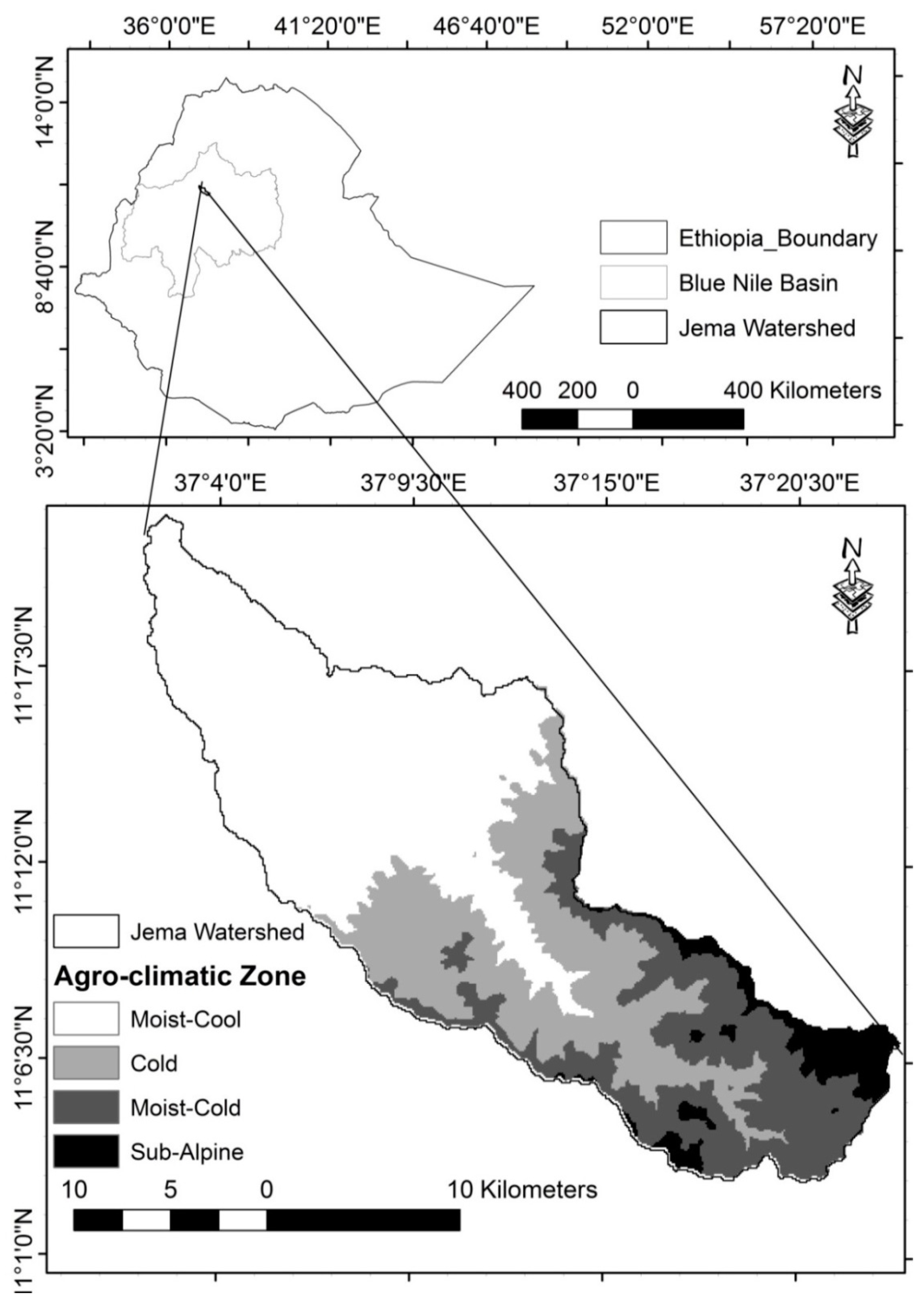
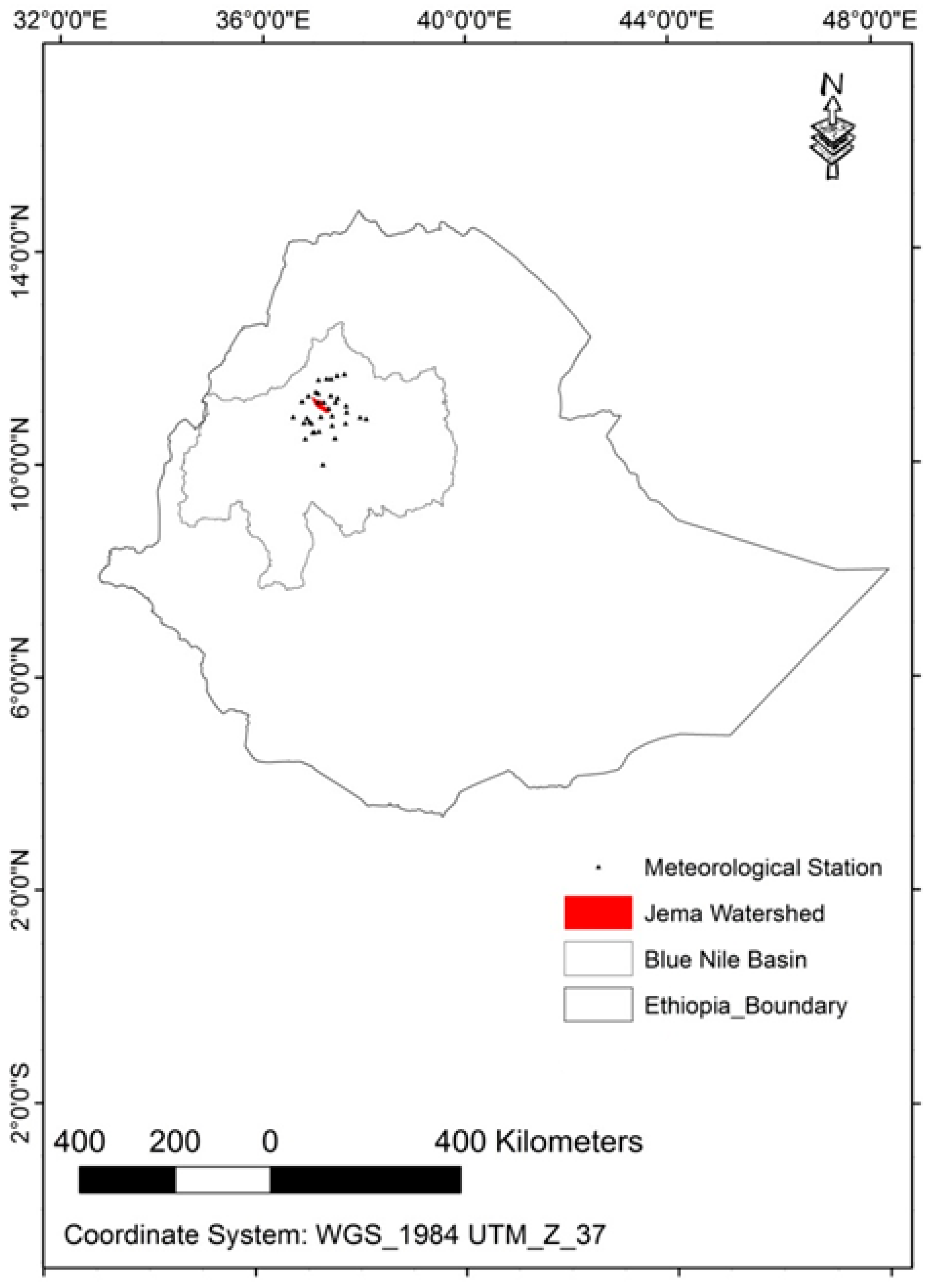
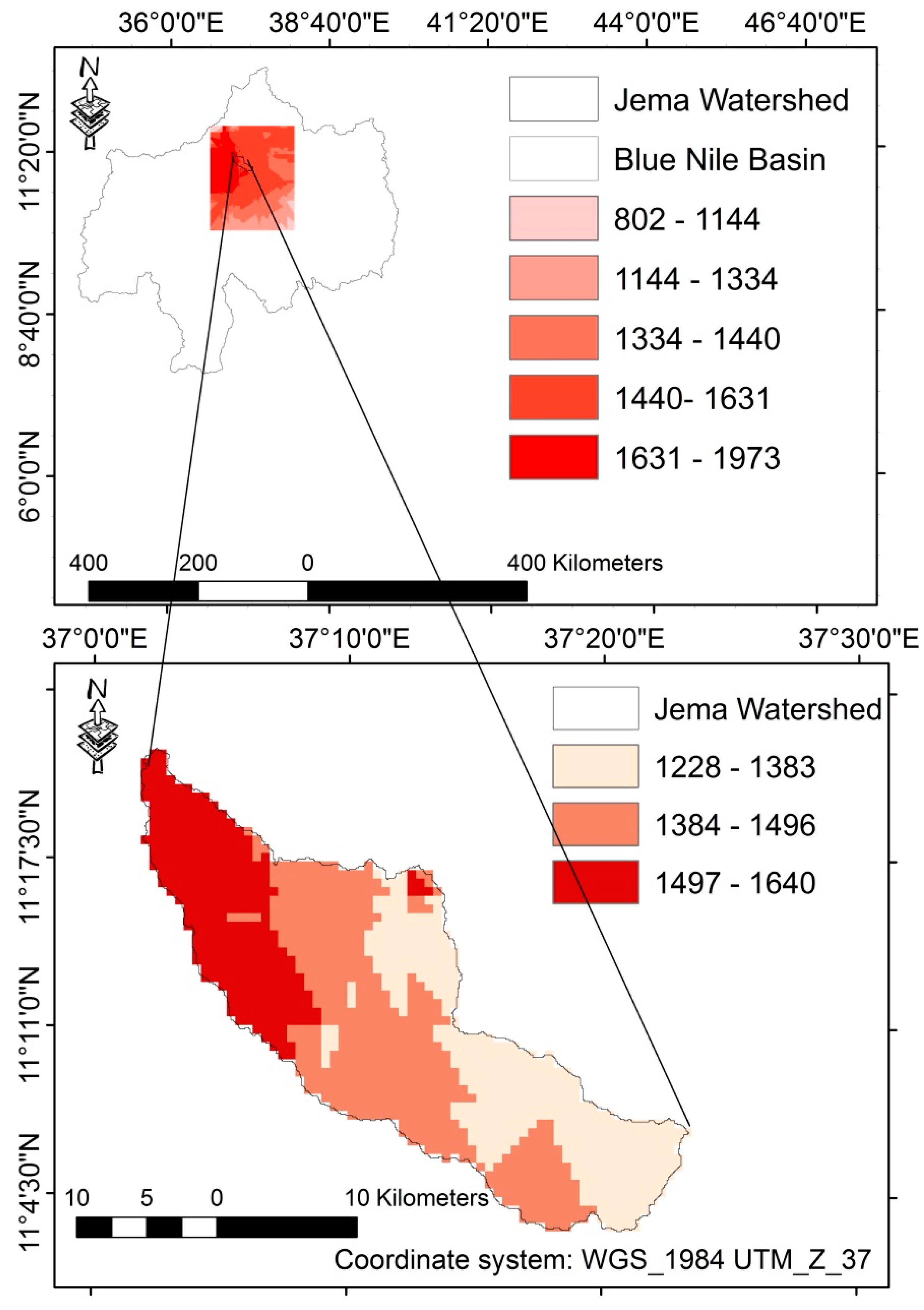
2.1. Description of the Study Area

As computed from a digital elevation model with 30-m resolution (DEM 30 m), the Jema watershed is situated at 11°22′0′′ N to 11°3′30′′ N and 37°2′0′′ E to 37°23′30′′E [36]. It is part of the northwestern highlands of Ethiopia in the Lake Tana sub-basin and the Upper Blue Nile River Basin (Figure 1). Its area covers 48,244.12 ha (~483 km2) and it has an elongated physical structure. The road line distance that it takes to get to the watershed is estimated to be 80 km south of Bahir Dar, the capital of the regional state, and 500 km north of Addis Ababa, the country’s capital. As stated in reference [37], 80% of Ethiopia’s farming activity is situated in the highlands.
Volcanic rocks of late Tertiary to Quaternary age dominate the geology of the watershed [38]. The site is characterized by a complex terrain with gentle slopes, a hilly landscape, and steep slopes. As computed from DEM 30 m, the elevation of the site ranges from 1895 to 3518 m a.s.l. (Figure 1). The elevation declines from southeast to northwest. The site is generally characterized by moist highlands [9,10]. Based on the local classification system [9], the site consists of moist-cool highlands (Weyina-Dega), cold highlands (Low-Dega), moist-cold highlands (High-Dega), and sub-alpine (Low-Wurch) ACZs. The area coverage of the agro-climatic zones of Jema watershed is presented in Table 1.
The slope of the watershed ranges from 0 to 45% (as generated from DEM 30 m). The steepness increases from northwest to southeast [36]. About 80% of the total rainfall occurs during summer (Kiremt) [39]. The MATRF is ~1400 mm [40]. On average, the monthly maximum temperature and monthly minimum temperature are ~25 °C and ~7 °C, respectively. The National Meteorological Agency of Ethiopia showed that the maximum temperature was recorded in March during spring (Belg) [40]. Heavy clay, clay, and clay loam were identified as the major texture classes of soil in the lower, middle, and upper parts of the watershed, respectively [36].
At the regional level (the Amhara Regional State), the population density is ~189.4 persons/km2 [41]. As stated in the work of [36], the livelihood of inhabitants is dependent on subsistence scale mixed farming; i.e., food crop production and livestock rearing. Farming heavily depends on the presence of a rainfed system with scanty small holding irrigation. The main livestock types include cattle, sheep, goats, horses, donkeys, mules and poultry. The land use/land cover (LULC) types at the site are cropland, grazing land, settlement land, bare land, bush land, wood land, riverine trees, water bodies, and forest land.

2.2. Datasets

Most of the Ethiopian meteorological datasets have been inconsistently recorded [7,40]. This was a big challenge for the climate variability analysis. The problem was more serious in ordinary (class 4 and 3) stations that are situated in rural villages and towns [40]. To fill this gap, the Ethiopian Meteorological Agency, in collaboration with International Research Institute for Climate and Society at Columbia University, USA, reconstructed the incomplete meteorological datasets using satellite observation records (NASA EOS mission, MODIS). Data calibration and validation were undertaken by Reading University, UK [7]. The reconstructed gridded data was collected from 1983 to 2010 at a spatial scale of 10 × 10 km2. With regard to the quality of the reconstructed datasets, the results showed a strong correlation (r = 0.80) between the station and satellite-derived data [7]. Accordingly, sample MATRF data of this study were collected from nearby 34 stations. Elevation (m) was another dataset that was generated from the DEM 30m. The source of this elevation data set was the United States Geological Survey (USGS).

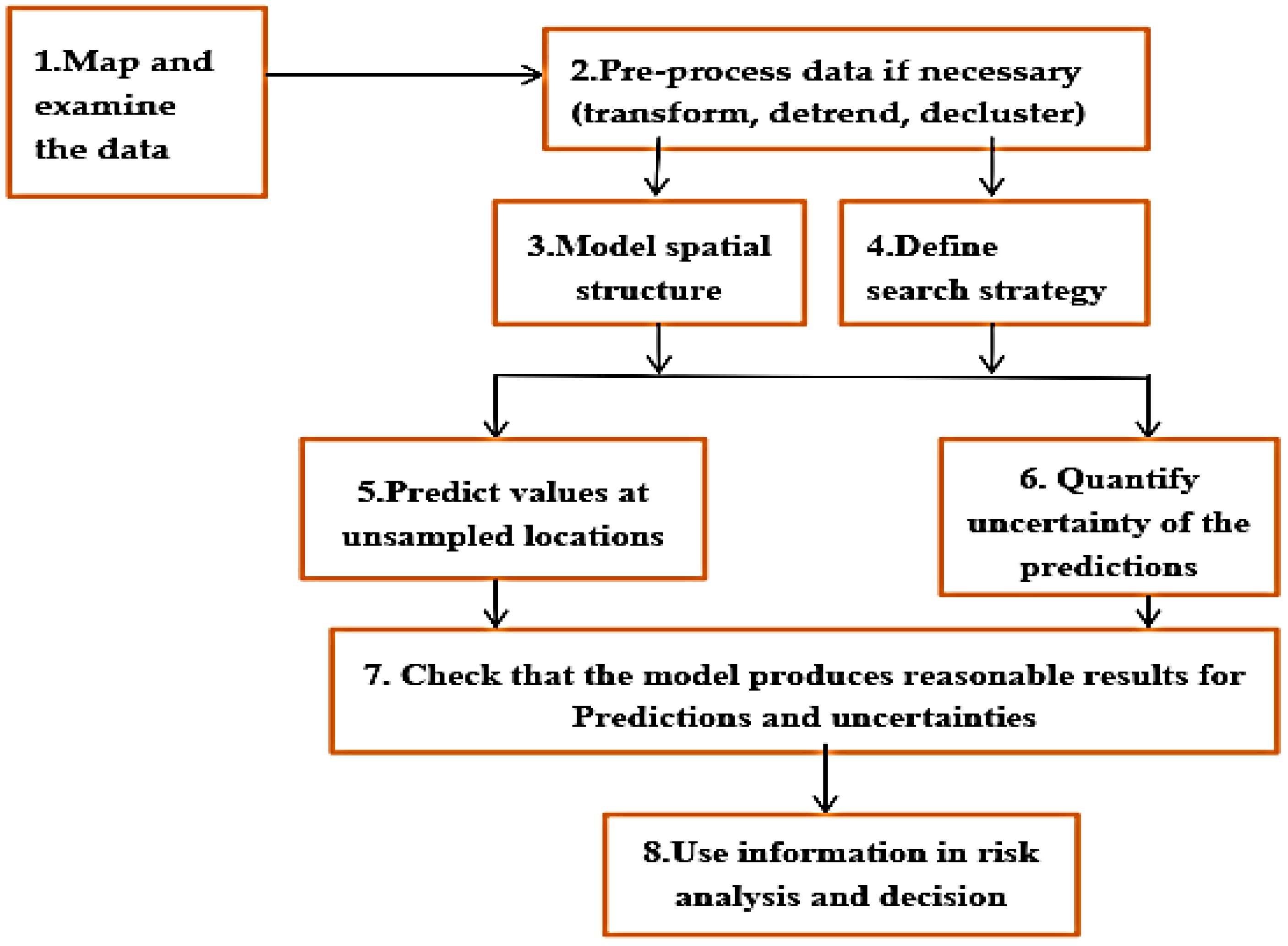
2.2.1. Methods of Spatial Estimation of Rainfall

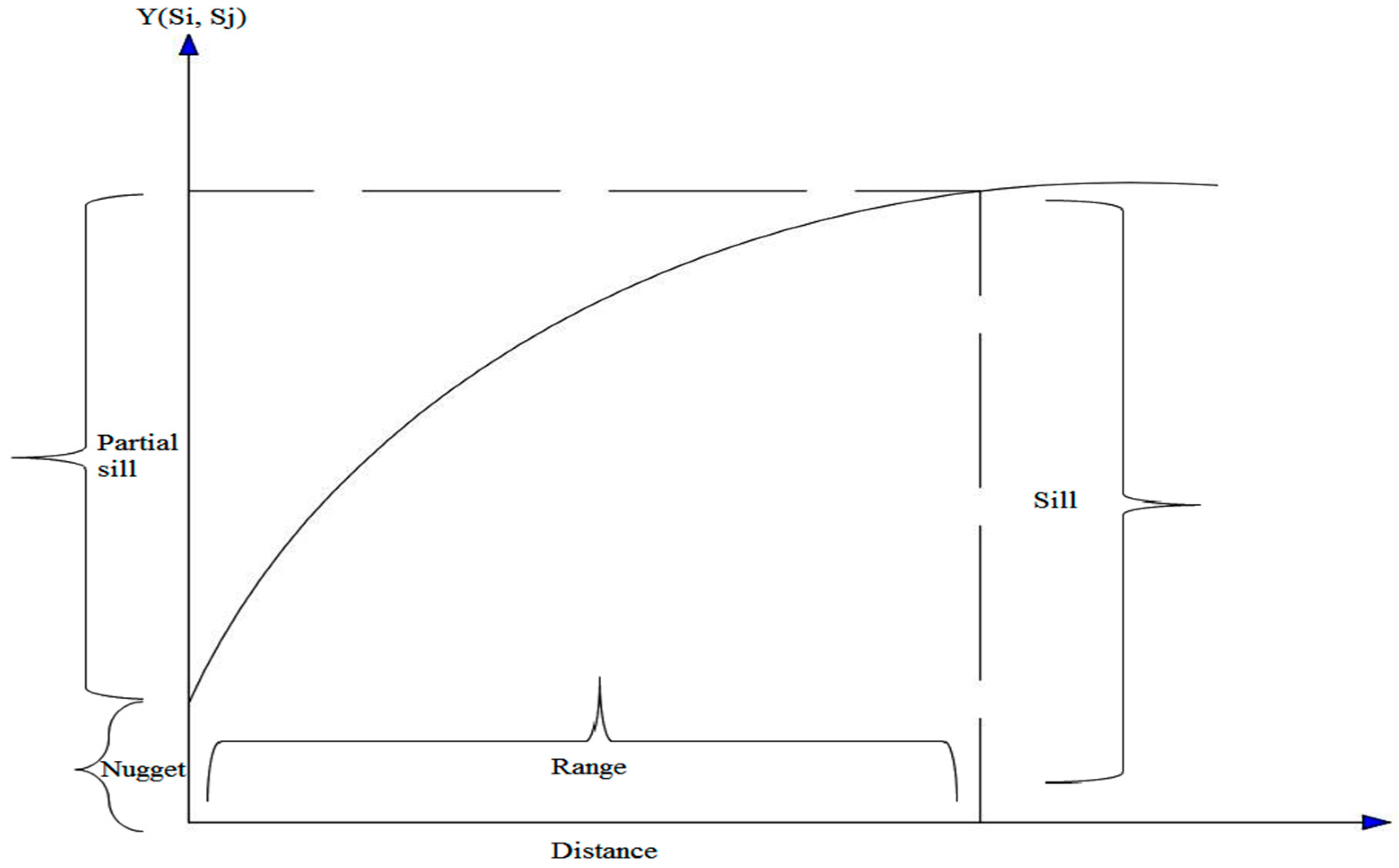
Exploring Geostatistical Functions

It is believed that spatial interpolation of the precipitation data inmountainous areas is technically challenging as it needs to be performed taking into consideration complex topography of the terrain [18]. Hence, in order to estimate the spatial distribution of the MATRF, it was essential to choose an appropriate geostatistical method. In the estimation analysis, the MATRF dataset was a predict and variable, whereas the elevation (m) dataset generated from the DEM 30m was an auxiliary variable.
The geospatial interpolation method can be used to characterize patterns of rainfall over various spatial scales, provided that the data are spatially dependent [13]. This method is more appropriate when a dataset exhibits a smooth and consistent pattern of spatial dependence within a given study area [42,43]. As part of an exploration of the geostatistical function, spatial autocorrelation needs to be assessed by applying the semivariogram function. This function is defined in Equation (1). If two locations, s1 and s2, are close to each other in terms of the distance measure of d(s1, s2), they are expected to be similar, so the difference in their values, Z(s1) − Z(s2), will be small. As s1 and s2 get farther apart, they become less similar, so the difference in their values, Z(s1) − Z(s2), becomes larger.
γ(s1,s2) = 1/2var (Z(s1) − Z(s2))
where, var is the variance; s is the observed location in terms of distance (d); and Z is the observed value of a given variable situated in a given location (geographical distance).
In a semivariogram model, one can notice that at a certain distance, the model levels out (Figure 2). The distance where the model first flattens out is known as the range. Sample locations separated by distances closer than the range are spatially auto-correlated, whereas locations farther apart than the range are not. The value that the semivariogram model attains at the range (the value on the y-axis) is called the sill. The partial sill is the sill minus the nugget. The nugget effect is attributed to spatial sources of variation at distances smaller than the sampling interval and/or measurement errors. Natural phenomena may vary spatially over a range of scales. A spatial variation at micro-scales smaller than the sampling distances may appear as part of the nugget effect. Accordingly, before collecting data, it is essential to gain some understanding of the scales of variation.
The lag size (spatial distance) to be determined in semivariogram modeling can affect the sill, nugget, partial sill, and range values, and ultimately, the performance of the whole interpolation method (Figure 2). For larger lag sizes, it is possible for short range spatial autocorrelation to be masked [13]. In the process of deciding the lag size, if the range of the fitted semivariogram model is very small relative to the extent of the empirical semivariogram, the lag size needs to be minimized. Conversely, if the range of the fitted semivariogram model is large relative to the extent of the empirical semivariogram, the lag size needs to be maximized. Depending on how well they fit the data, several semivariogram models (exponential, Gaussian, circular, and spherical) may be employed [44]. As a rule, a semivariogram model that fits empirical data should pass as closely as possible to the mean values, and/or it should pass the center of the cloud, and/or it should pass as closely as possible to the lines (Figure 2). The steeper the curves near the origin of the graph, the more influence the closest neighbors will have on the prediction [45].
Moreover, the performances of circular versus spherical functions, exact versus inexact smoothing, and local versus global trend geostatistical functions were examined in this study. The spherical (directional effect) function is expected to be appropriate for interpolating environmental variables that show directional variability [45]. However, the geographical scale of analysis, the degree of variability of predictor variables, and the existence of multiple geospatial features, like exponential and non-linear variation and global and local trends, could reverse the result [13]. For example, local trends perform better in situations where local variability (multiple trends) exists [43].
The ordinary kriging (OK), simple kriging (SK), universal kriging (UK), disjunctive kriging (DK), (ordinary cokriging (OCK), inverse distance weighting (IDW), (global polynomial interpolation (GPI), local polynomial interpolation (LPI), and radial basis function (RBF) interpolation models were examined in this study. The models were run with the help of ArcMap 10.2 software. The first five models are stochastic, whereas the last four models are deterministic (mathematical) in nature [13].
IDW estimates cell values by averaging the values of sample data points in the neighborhood of each processing cell. The closer a point is to the center of the cell being estimated, the more influence, or weight; it has in the averaging process. While GPI fits a polynomial to the entire surface, LPI fits many polynomials; each within specified overlapping neighborhoods.The search neighborhood can be defined by using the size and shape, number of neighbors, and sector configuration. Being exact interpolators, the RBF methods differ from the global and local polynomial interpolators, which are exact interpolators that do not require the surface to pass through the measured points. When comparing RBF to IDW (which is also an exact interpolator), IDW will never predict values above the maximum measured value or below the minimum measured value [13]. Kriging is an advanced geostatistical procedure that generates an estimated surface from a scattered set of points with z-values. Kriging models differ from each other in the trend in terms of the random function that is considered in their algorithm [11]. For instance, SK considers the trend to be known and constant all over the study area. The trend is unknown in the OK and is considered to fluctuate locally, maintaining the stationarity within the local neighborhood. The UK considers that the trend smoothly varies within each local neighborhood and is modeled as a linear combination of functions of the spatial coordinates. If auxiliary information is considered together with the primary data, some multivariate extension of kriging (cokriging) could result in better estimates [11].
Unlike the other methods, stochastic methods enable the user to analyze error terms. It is only in stochastic methods that both the accuracy and precision of predictions can be analyzed (Figure 3). Some of the stochastic models work best for environments with irregular variability, whereas others work better for regular variability [13]. Similar description about the models is also noted in the ArcMap program.

Evaluating Model Performance

The models were evaluated with a comparison of the possible committed error values including mean error (ME), root-mean-square standardized error (RMSSE), root-mean-square error (RMSE), mean standard error (MSE), and standardized root-mean-square error (SRMSE) (2)–(6)). The evaluation involved the use of the leave-one-out cross validation geostatistical technique with a confidence interval of 95%. This technique uses all of the data to estimate the trend and autocorrelation models. The technique removes each data location, one at a time, and predicts the associated data value. In general terms, the best model is the one that has the smallest root-mean-squared prediction error, the mean standard error nearest to the root-mean-squared prediction error, the standardized mean nearest to zero, and the standardized root-mean-squared prediction error nearest to one [46]. ME and RMSSE are used to identify the most optimal model, whereas RMSE and ASE are used to identify the most valid model. These geostatistical methods have been used in several studies [47,48]. The variables are defined in Equations (2)–(6).
ME = 1 n i = 1 n   ( p i   o i )
RMSSE = [ 1 n i = 1 n ( p si o si   ) 2 ] 1 / 2
RMSE = [ 1 n i = 1 n ( p i o i   ) 2 ] 1 / 2
MSE = [ 1 n i = 1 n ( p i ( i = 1 n p i ) / n ) 2 ] 1 / 2
SRMSE = R M S E E s t i m a t e d m a x E s t i m a t e d m i n
where ME is the mean error; RMSSE is the root-mean-square standardized error; RMSE is the root-mean-square error; MSE is the mean standard error; n is the number of observations or samples; o Is the observed value at place i; p is the predicted/estimated value at place i; osi is the standardized observed value at place i; psi is the standardized predicted/estimated value at place I; and SRMSE is the standardized root-mean-square error; E s t i m a t e d m a x is the maximum estimated value of rainfall; E s t i m a t e d m i n is the minimum estimated value of rainfall.
As part of validating the performance of interpolation models, a bias of estimators was also computed. The raster layer of the rainfall value estimation, summary table value of estimation error and error graph were used to preset the result of the study; whereas histogram was used to describe the data set. For the sake of simplicity, it was preferred to present a table value of mean error for all of the interpolation models; and raster layer, error scatter plot and bias table only for the model that showed the best performance in the process of estimation. The summary of the procedure that was followed in interpolating MATRF is presented in Figure 3.

3. Results and Discussion

The sample stations considered for the interpolation were located in the north, south, east, and west directions of the Jema watershed (Figure 4). The samples were situated within a ~40 km radius of the center of the watershed. As shown in Table 2, the skewness coefficient value becomes 0.4 after log transformation. Although data normality is not a requirement in the application of kriging models, the descriptive statistics implies the presence of normal distribution in the sampled data set.

3.1. An Appropriate Geostatistical Function

Initially, due to the existence of a poor correlation between the observed MATRF values (as a predictand variable) and observed elevation values (as a covariable), it was planned that only kriging methods would be employed. In the trend function (least square method) analysis, the value was weak (R2 = 0.07) (Figure 5). On the other hand, in the neighborhood search analysis, a pattern was observed in the spatial distribution of MATRF and elevation. Mainly because of this observation, it was determined that it was reasonable to incorporate elevation as a covariable to test the performance of the cokriging model in estimating the MATRF of the watershed.
In the process of interpolating the predictand variable, specifically, during the neighborhood search analysis step, it was possible to detect a kind of MATRF spatial pattern that followed the variation in elevation in some corners of the krigged surface. Accordingly, it was reasonable to test the cokriging model in addition to kriging models.

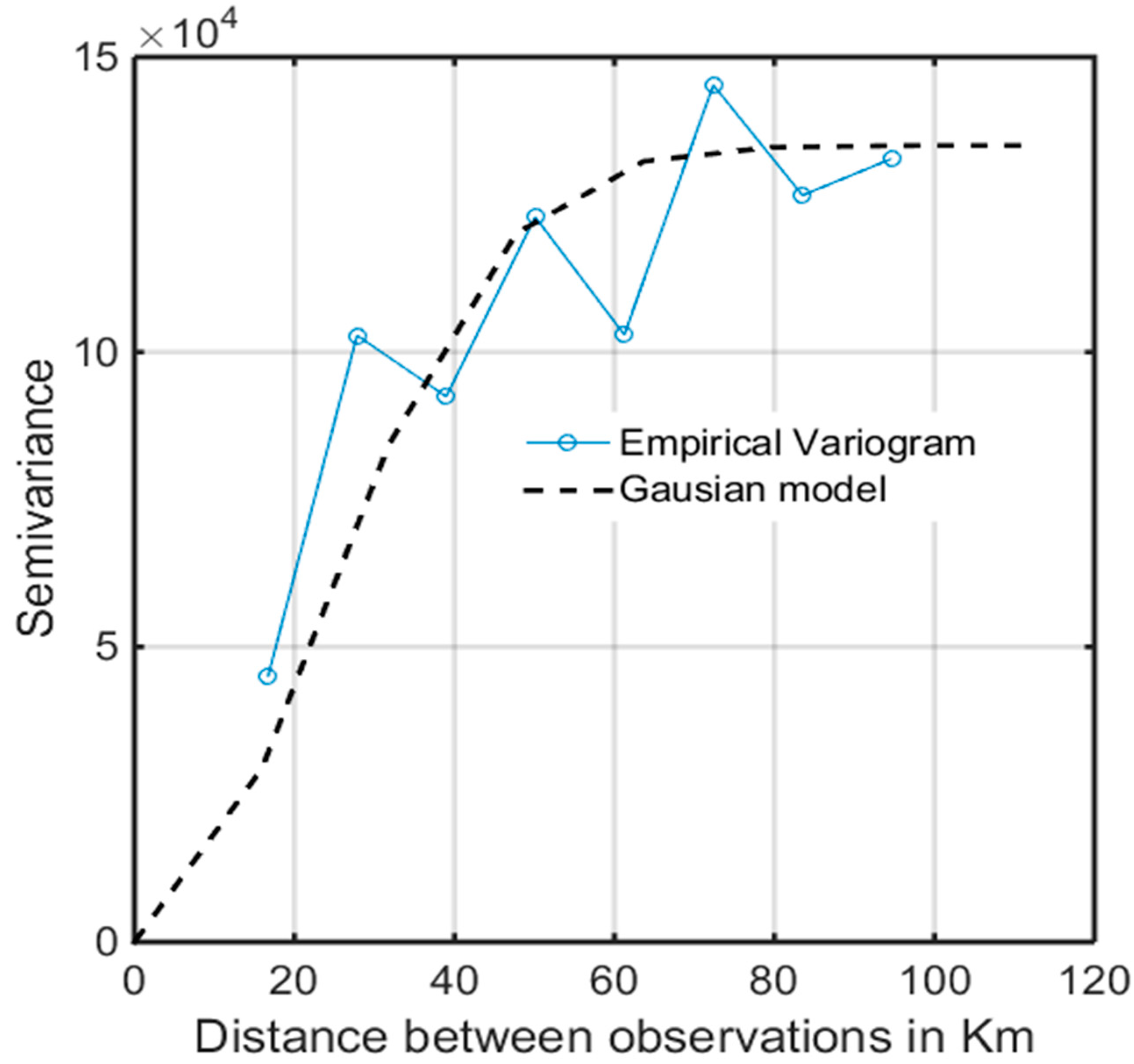
3.1.1. Geostatistical Autocorrelation

In the semivariogram modeling, Gaussain model became the best fit to the spatial autocorrelation of the observed average MATRF data set. The model (trend line) passed through the binned value, and the mean values were distributed near the mode line. As presented in Figure 6, semivariogram parameters (nugget effect = ~0, sill = ~14, range = ~100 km, lag size = 20 km, number of lags = 6) could be obtained in most of the kriging and cokriging models.

3.1.2. Neighborhood Searching and Directional Influence

Interpolation models can be used effectively with local polynomial trend removal (local variation), a non-power function (non-weighted mean) and 6 to 2 maximum-minimum local neighbor searches. The sector type was found at 4 and 45 degrees with a major range of 0.66 km in the east to west direction and a minor range of 0.28 km in the north to west direction. In the geostatistical analysis, an anisotropy effect was identified with an elliptical neighborhood search strategy shape at the scale of the watershed, the MATRF declines from northwest to southeast, i.e., from areas of lower elevation to higher elevation (Figure 7 and Figure 8). However, for the entire sample site, there was a weak spatial association between the MATRF and elevation values (Figure 5). The results showed the existence of direction influence and non-linear smooth variation in the MATRF distribution for the entire interpolated (sample) site. The result shows the existence of a number of ups and downs in the spatial distribution of the MATRF throughout the whole sample site.
The result in Figure 8 implies that the equatorial (southeasterly) winds from the Indian Ocean enhance the MATRF received in the main rainy season (Kiremt) to the entire sample site—part of the northwestern highlands of Ethiopia. Accordingly, the highlands in the west of the sample site are situated alongthe wind-ward side (of the southeasterlies) and receive relatively higher MATRF.
Similar to the result of this study, references [30,49] found that the MATRF declines from northwest to southeast. On the other hand, the finding of this study is contrary to previous observations made in Ethiopia [10,39] which showed an increase in the MATRF with elevation. However, this study shares the general conclusions of references [10,39] that Ethiopian highland rainfall is influenced by topography. That is, due to the distribution of the MATRF, the mountains create wind-ward and lee-ward side effects.

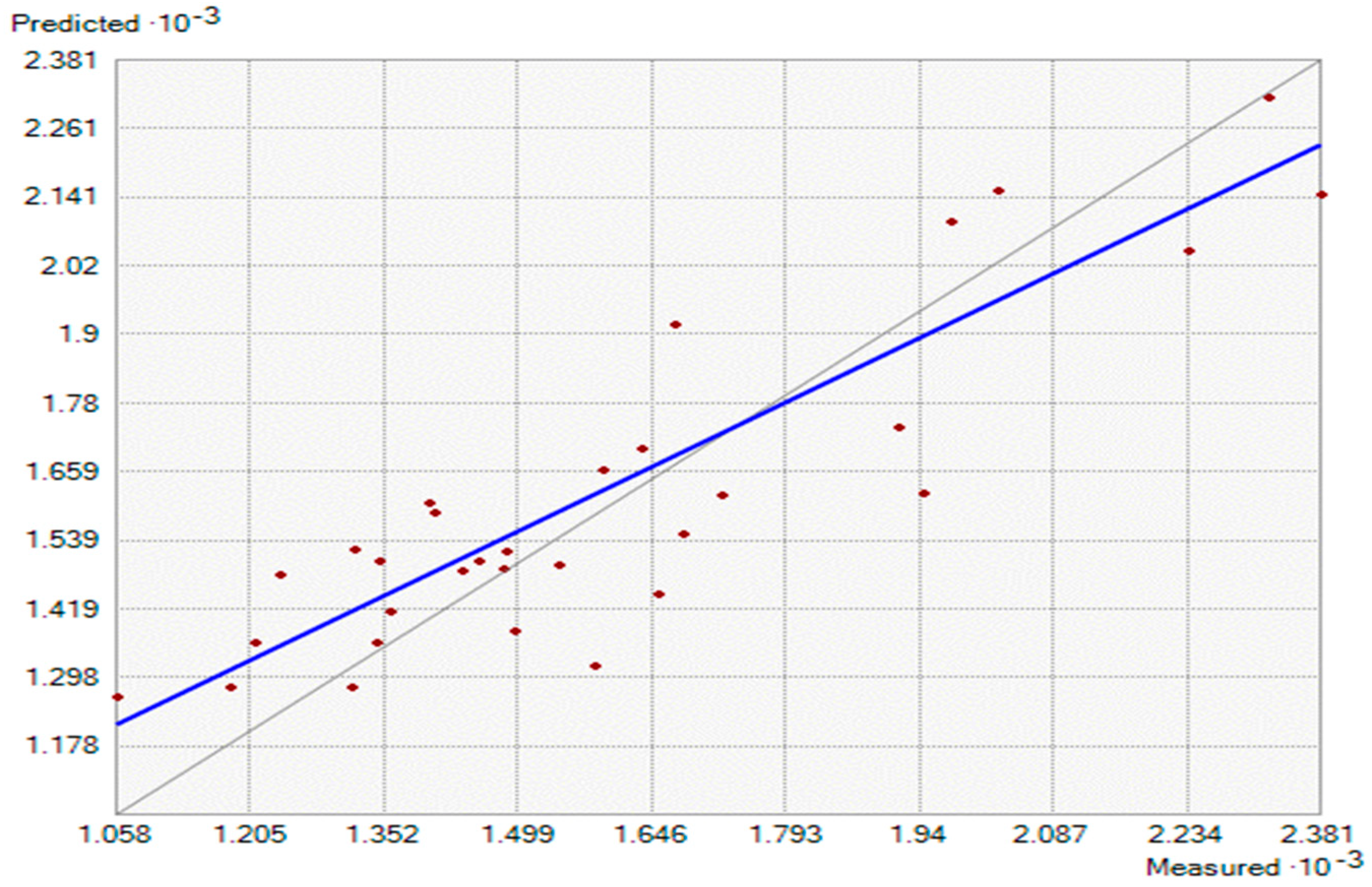
3.1.3. Cross Validation Statistics

The smallest RMSE (157.9 mm) and the smallest range statistic between RMSE and ASE (i.e., the range between 157.9 and 231.8) were observed in the OCK model (Table 3). The standardized value of the indicated RMSE would be 0.127. The predictive power of the model was 87.3%. Compared to the other models, in terms of estimating rainfall value, OCK was found to be the most appropriate for the study site. It was shown to enhance the predictive power of estimation in the range of 1.05% (15 mm) to 11% (134 mm). Furthermore, in terms of precision, the RMSSE values indicated that all models were similar. The same multivariate model showed the best precision value (0.72 mm), which is the lowest among others (Table 3). As presented in Figure 6, OCK became the most appropriate model at values of the following semivariogram parameters (nugget effect = ~0, sill = ~14, range = ~100 km, lag size = 20 km, number of lags = 6). The indicated nugget effect implies the absence of sampling interval and/or measurement errors. As part of validating the estimation, bias was computed considering the observed and estimated MATRF values. The lowest bias is observed in OCK model (bias = 0.26). The error graph of OCK is presented in Figure 9. Similarly, the other stochastic interpolation models could also perform better at the same values of the indicated parameters.
Because of the presence of the east to west and southeast to northwest spatial pattern for elevation and MATRF respectively, the use of topography as a covariable improved the performance of the multivariate geostatistical estimation techniques. This estimation was observed in a situation where the trend line values between the MATRF and the longitude coordinate (east–west direction) was found to be average (R2 = 0.34) (Figure 7). Elevation, as a covariable, played a role in minimizing the degree of error estimation. It happened in the absence of a statistical association between the MATRF and elevation. Hence, when choosing environmental a covariable, in addition to the correlation strength between the predicted variable and covariable, one may need to look at the nugget effect of the cross semivariogram between rainfall and elevation. Furthermore, the spatial association that was not detected by the simple non-geospatial correlation analysis (Figure 5 and Figure 7) could be observed by applying a kriging geostatistical analysis (Table 4, Figure 8 and Figure 9).
In congruence with the results of the new study, the benefit of using elevation data to estimate the spatial distribution of precipitation was observed in previous study [50]. As stated by [51], elevation-dependent spatial interpolators were accurate. In reference [21], the global digital elevation model was incorporated as an ancillary variable into the spatial prediction of the average annual precipitation using the geostatistical method. For this reason, the geostatistical analysis could perform better than other deterministic interpolation techniques for rain gauge data. As noted by [52] interpolation methods provide similar spatial distributions of rainfall wherever observation network is dense. However, the inclusion of geographical variables to the interpolation method should improve estimates in areas where the observation network density is low.

3.2. The Estimated MATRF among the Agro-Climatic (Elevation) Zones

Based on the extracted krigged values, the Jema watershed receives between 1228 and 1640 mm of MATRF (Table 4 and Figure 8).
Finally, analysis of variance (ANOVA) was used to test whether there was a statistical difference between the MATRF values among the ACZS. The two-tailed p-value (0.04) was below 0.05. Thus, H0 (the null hypothesis stating that there is no significant variation between groups) was rejected. This indicates the existence of a significant variation in the MATRF among the ACZs of the watershed.
Similar to the argument of reference [30] and in contrast to the general observation of reference [9], the results of this study showed a decline in the amount of MATRF from the northwest (lower elevation) to the southeast (higher elevation) of the Jema watershed. Nevertheless, the same pattern of MATRF was not observed all over the study corners that were included in the interpolated surfaces. The temporal and spatial variation of the mean rainfall of Ethiopia is mainly determined by its topography [10]. Another study explained that for large mountain ranges, precipitation is maximized over the wind-ward slopes, whereas for smaller hills, the maximum tends to occur nearer the crest [50]. Ethiopian rainfall occurs in summer and spring and is mainly driven by the westerly winds coming from the Atlantic Ocean and the easterly winds coming from the Indian Ocean [30]. Mainly because of this fact, the MATRF over the basin decreases from southwest to northeast Ethiopia [31]. On the other hand, [10,30] indicated that the MATRF increases with elevation in Ethiopia.
As stated by [53,54], the summer rainfall in Ethiopia is controlled by several climatological factors, including a seasonal northward advance of the inter-tropical convergence zone (ITCZ) which persists over Ethiopia and the southerly/southwesterly cross-equatorial moisture flow from the Southern Indian Ocean. For this reason, places situated at higher elevations (above 2000 m a.s.l.) are expected to receive a lower MATRF than the lower elevated areas.
Based on the MATRF received, the study watershed could be categorized as a moist highland region. This categorization is supported by [10]. In terms of the total moisture obtained from rainwater, the farming systems of the ACZs located at the lower elevations have an advantage. This might be true with respect to the rainwater harvesting potential that could be utilized as a backup in times of unexpected shortages of rainwater. As stated in the Plan for Accelerated and Sustainable Development to End Poverty (PASDEP), the enhancement of water harvesting and irrigation potential is a key priority in the agricultural sector to allow adaptation to climate stresses like rainfall variability and temperature change [41].

4. Conclusions

Geostatistical methods can be used to estimate rainfall values to areas where rain gauge data is lacking. In the case of the Jema watershed, the cokriging interpolation method, specifically the ordinary cokriging model, was shown to be superior to the deterministic and kriging methods. The MATRF across the Jema watershed ranges from 1228 to 1640 mm. Elevation contributes as a variable to the estimation of the MATRF. Moreover, the MATRF showed a spatial association with longitudinal coordinate values, i.e., in the northwest to southeast direction. The rainfall declines from northwest to southeast, i.e., from lower to higher elevations. It happens in a situation where a weak trendline association exists between elevation and MATRF. The association between the MATRF and elevation is not straightforward in the entire sample sites. That is, the spatial pattern of the MATRF does not follow the same pattern across the entire sample site where the current study watershed is situated. Overall, in river basins with complex topographies, the estimation of MATRF needs a micro-scale, watershed-level analysis employing a local trend geostatistical model.

Author Contributions

Conceptualization, M.A.T.; Formal analysis, M.A.T.; Investigation, M.A.T.; Methodology, M.A.T.; Supervision, B.S.B., B.F.Z., S.G.S. and Y.G.S.; Writing–original draft, M.A.T.

Funding

Belmont Forum: via NSF award ICER-1624335, Addis Ababa University, and Bahir Dar University, Ethiopia.

Acknowledgments

Florida International University, USA, is appreciated for hosting the senior author as a visiting scholar.

Conflicts of Interest

The authors declare no conflicts of interest.

References

  1. Sawin, J. National policy instruments: Policy lessons for the advancement & diffusion of renewable energy technologies around the world. In Renewable Energy. A Global Review of Technologies, Policies and Markets; Routledge: Abingdon, UK, 2006. [Google Scholar]
  2. UNFCCC. Investment and Financial Flows to Address Climate Change; UNFCCC: Bonn, Germany, 2007. [Google Scholar]
  3. Stern, N. The Economics of Climate Change: The Stern Review; Cambridge University Press: Cambridge, UK, 2007. [Google Scholar]
  4. Anita, W.; Dominic, M.; Neil, A. Climate Change and Agriculture Impacts, Adaptation and Mitigation: Impacts, Adaptation and Mitigation; OECD Publishing: Paris, France, 2010. [Google Scholar]
  5. Beyene, T.; Lettenmaier, D.P.; Kabat, P. Hydrologic impacts of climate change on the Nile River Basin: Implications of the 2007 IPCC scenarios. Clim. Chang. 2010, 100, 433–461. [Google Scholar] [CrossRef]
  6. Conway, D. From headwater tributaries to international river: Observing and adapting to climate variability and change in the Nile basin. Glob. Environ. Chang. 2005, 15, 99–114. [Google Scholar] [CrossRef]
  7. Mengistu, D.; Bewket, W.; Lal, R. Recent spatiotemporal temperature and rainfall variability and trends over the Upper Blue Nile River Basin, Ethiopia. Int. J. Climatol. 2014, 34, 2278–2292. [Google Scholar] [CrossRef]
  8. Zaitchik, B.F.; Simane, B.; Habib, S.; Anderson, M.C.; Ozdogan, M.; Foltz, J.D. Building Climate Resilience in the Blue Nile/Blue Nile Highlands: A Role for Earth System Sciences. Public Health 2012, 9, 435–461. [Google Scholar]
  9. MoARD (Ministry of Agriculture and Rural Development, Ethiopia). Agroecologicalzonations of Ethiopia; MoARD: Addis Ababa, Ethiopia, 2000. [Google Scholar]
  10. Hurni, H. Agroecological belts of Ethiopia: Explanatory notes on three maps at a scale of 1: 1,000,000; Soil Conservation Research Program of Ethiopia: Addis Ababa, Ethiopia, 1998; p. 31. [Google Scholar]
  11. Goovaerts, P. Geostatistical approaches for incorporating elevation into the spatial interpolation of rainfall. J. Hydrol. 2000, 228, 113–129. [Google Scholar] [CrossRef] [Green Version]
  12. Diodato, N. The influence of topographic co-variables on the spatial variability of precipitation over small regions of complex terrain. Int. J. Climatol. 2005, 25, 351–363. [Google Scholar] [CrossRef] [Green Version]
  13. Li, J.; Heap, A.D. A Review of Spatial Interpolation Methods for Environmental Scientists; Geoscience Australia Record: Symonston, Australian, 2008; Volume 23, p. 137. [Google Scholar]
  14. Yang, Q.; Ma, Z.-G.; Chen, L. A Preliminary Analysis of the Relationship between Precipitation Variation Trends and Altitude in China. Atmos. Ocean. Sci. Lett. 2011, 4, 41–46. [Google Scholar]
  15. Roe, G.H. Orographic precipitation. Annu. Rev. Earth Planet. Sci. 2005, 33, 645–671. [Google Scholar] [CrossRef]
  16. Plouffe, C.C.; Robertson, C.; Chandrapala, L. Comparing interpolation techniques for monthly rainfall mapping using multiple evluation criteria and auxiliary data sources: A case study of Sri Lanka. Environ. Model. Softw. 2015, 67, 57–71. [Google Scholar] [CrossRef]
  17. Xuan, W.; Fu, Q.; Qin, G.; Zhu, C.; Pan, S.; Xu, Y.P. Hydrological Simulation and Runoff Component Analysis over a Cold Mountainous River Basin in Southwest China. Water 2018, 10, 1705. [Google Scholar] [CrossRef]
  18. Gilewski, P.; Nawalany, M. Inter-Comparison of Rain-Gauge, Radar, and Satellite (IMERG GPM) Precipitation Estimates Performance for Rainfall-Runoff Modeling in a Mountainous Catchment in Poland. Water 2018, 10, 1665. [Google Scholar] [CrossRef]
  19. Hirpa, F.A.; Gebremichael, M.; Hopson, T. Evaluation of high-resolution satellite precipitation products over very complex terrain in Ethiopia. J. Appl. Meteorol. Climatol. 2010, 49, 1044–1051. [Google Scholar] [CrossRef]
  20. Emadi, M.; Shahriari, A.R.; Sadegh-Zadeh, F.; JaliliSeh-Bardan, B.; Dindarlou, A. Geostatistics-based spatial distribution of soil moisture and temperature regime classes in Mazandaran province, Northern Iran. Arch. Agron. Soil Sci. 2016, 62, 502–522. [Google Scholar] [CrossRef]
  21. Bajat, B.; Pejović, M.; Luković, J.; Manojlović, P.; Ducić, V.; Mustafić, S. Mapping average annual precipitation in Serbia (1961–1990) by using regression kriging. Theor. Appl. Climatol. 2013, 112, 1–13. [Google Scholar] [CrossRef]
  22. Diro, G.T.; Grimes, D.I.F.; Black, E.; O’Neill, A.; Pardo-Iguzquiza, E. Evaluation of reanalysis rainfall estimates over Ethiopia. Int. J. Climatol. 2009, 29, 67–78. [Google Scholar] [CrossRef] [Green Version]
  23. Martínez-Cob, A. Estimation of mean annual precipitation as affected by elevation using multivariate geostatistics. Water Resour. Manag. 1995, 9, 139–159. [Google Scholar] [CrossRef] [Green Version]
  24. Gouvas, M.; Sakellariou, N.; Xystrakis, F. The relationship between altitude of meteorological stations and average monthly and annual precipitation. Stud. Geophys. Geod. 2009, 53, 557–570. [Google Scholar] [CrossRef]
  25. Buytaert, W.; Celleri, R.; Willems, P.; De Bievre, B.; Wyseure, G. Spatial and temporal rainfall variability in mountainous areas: A case study from the south Ecuadorian Andes. J. Hydrol. 2006, 329, 413–421. [Google Scholar] [CrossRef] [Green Version]
  26. Dingman, S.L.; Seely-Reynolds, D.M.; Reynolds, R.C. Application of kriging to estimating mean annual precipitation in a region of orographic influence 1. J. Am. Water Resour. Assoc. 1988, 24, 329–339. [Google Scholar] [CrossRef]
  27. Hutchinson, M.F. Interpolating mean rainfall using thin plate smoothing splines. Int. J. Geog. Inf. Syst. 1995, 9, 385–403. [Google Scholar] [CrossRef] [Green Version]
  28. Phillips, D.L.; Dolph, J.; Marks, D. A comparison of geostatistical procedures for spatial analysis of precipitation in mountainous terrain. Agric. For. Meteorol. 1992, 58, 119–141. [Google Scholar] [CrossRef]
  29. Sevruk, B. Regional dependency of precipitation-altitude relationship in the Swiss Alps. In Climatic Change at High Elevation Sites; Springer: Dordrecht, The Netherlands, 1997; pp. 123–137. [Google Scholar]
  30. Conway, D. The climate and hydrology of the Upper Blue Nile River. Geogr. J. 2000, 166, 49–62. [Google Scholar] [CrossRef]
  31. Seleshi, Y.; Zanke, U. Recent changes in rainfall and rainy days in Ethiopia. Int. J. Climatol. 2004, 24, 973–983. [Google Scholar] [CrossRef] [Green Version]
  32. Bewket, W. Rainfall variability and agricultural vulnerability in the Amhara region, Ethiopia. Ethiop. J. Dev. Res. 2008, 29, 1–34. [Google Scholar] [CrossRef]
  33. Haile, A.T.; Rientjes, T.; Gieske, A.; Gebremichael, M. Rainfall variability over mountainous and adjacent lake areas: The case of Lake Tana basin at the source of the Blue Nile River. J. Appl. Meteorol. Climatol. 2009, 48, 1696–1717. [Google Scholar] [CrossRef]
  34. Desta, L.; Carucci, V.; Wendem-Agenehu, A.; Abebe, Y. Community Based Participatory Watershed Development: A Guideline; Ministry of Agriculture and Rural Development: Addis Ababa, Ethiopia, 2005. [Google Scholar]
  35. Simane, B.; Zaitchik, B.F.; Foltz, J.D. Agroecosystem specific climate vulnerability analysis: Application of the livelihood vulnerability index to a tropical highland region. In Mitigation and Adaptation Strategies for Global Change; Springer: Berlin, Germany, 2016; Volume 21, pp. 39–65. [Google Scholar]
  36. Taye, M.; Simane, B.; Selsssie, Y.G.; Zaitchik, B.; Setegn, S. Analysis of the Spatial Variability of Soil Texture in a Tropical Highland: The Case of the Jema Watershed, northwestern Highlands of Ethiopia. Int. J. Environ. Res. Public Health 2018, 15, 1903. [Google Scholar] [CrossRef]
  37. Economy, C.R. Ethiopia’s Climate Resilient Green Economy: Green Economy Strategy; FDRE: Addis Ababa, Ethiopia, 2011. [Google Scholar]
  38. Poppe, L.; Frankl, A.; Poesen, J.; Admasu, T.; Dessie, M.; Adgo, E.; Deckers, J.; Nyssen, J. Geomorphology of the Lake Tana basin, Ethiopia. J. Maps 2013, 9, 431–437. [Google Scholar] [CrossRef] [Green Version]
  39. Agreement, A.A.; Virus, B.B.; Certificate, C.C.; Di ammonium Phosphate, D.A.; Authority, E.E.; Assessment, E.E.; Authority, E.E.; Action, E.E.; Authority, E.E.; Authority, E.E.; et al. Convention on Biological Diversity (CBD) Ethiopia’s 4th Country Report; Institute of Biodiversity Conservation: Addis Ababa, Ethiopia, 2009. [Google Scholar]
  40. NMA (National Meteorological Agency, Ethiopia). Initial National Communication of Ethiopia to the United Nations Framework Convention on Climate Change (UNFCCC); NMA: Addis Ababa, Ethiopia, 2007. [Google Scholar]
  41. BOFED (Bureau of Federal Economic Development). Population Affaires Core Process Based on 2012 Inter-Censal Survey. Amhara National Regional State Development Indicator; BOFED: Bahir Dar, Ethiopia, 2014; p. 15. [Google Scholar]
  42. Mohammad, Z.M.; Taghizadeh-Mehrjardi, R.; Akbarzadeh, A. Evaluation of geostatistical techniques for mapping spatial distribution of soil pH, salinity and plant cover affected by environmental factors in Southern Iran. Notulae Sci. Biol. 2010, 2, 92–103. [Google Scholar]
  43. Webster, R.; Oliver, M.A. Geostatistics for Environmental Scientists; John Wiley & Sons: Hoboken, NJ, USA, 2007. [Google Scholar]
  44. Jarvis, A.; Reuter, H.I.; Nelson, A.; Guevara, E. Hole-Filled SRTM for the Globe Version 4; University of Twente: Enschede, The Netherlands, 2008. [Google Scholar]
  45. Bachmaier, M.; Backes, M. Variogram or semivariogram? Understanding the variances in a variogram. Precis. Agric. 2008, 9, 173–175. [Google Scholar] [CrossRef]
  46. Robinson, T.P.; Metternicht, G. Testing the performance of spatial interpolation techniques for mapping soil properties. Comput. Electron. Agric. 2006, 50, 97–108. [Google Scholar] [CrossRef]
  47. Johnston, K.; VerHoef, J.M.; Krivoruchko, K.; Lucas, N. Using ArcGIS Geostatistical Analyst; Esri: Redlands, CA, USA, 2001. [Google Scholar]
  48. Setegn, S.G.; Rayner, D.; Melesse, A.M.; Dargahi, B.; Srinivasan, R. Impact of climate change on the hydroclimatology of Lake Tana Basin, Ethiopia. Water Resour. Res. 2011, 47. [Google Scholar] [CrossRef] [Green Version]
  49. Levin, N.E.; Zipser, E.J.; Cerling, T.E. Isotopic composition of waters from Ethiopia and Kenya: Insights into moisture sources for Eastern Africa. J. Geophys. Res. Atmos. 2009, 114. [Google Scholar] [CrossRef]
  50. Lloyd, C.D. Assessing the effect of integrating elevation data into the estimation of monthly precipitation in Great Britain. J. Hydrol. 2005, 308, 128–150. [Google Scholar] [CrossRef]
  51. De Amorim Borges, P.; Franke, J.; da Anunciação, Y.M.; Weiss, H.; Bernhofer, C. Comparison of spatial interpolation methods for the estimation of precipitation distribution in Distrito Federal, Brazil. Theor. Appl. Climatol. 2016, 123, 335–348. [Google Scholar] [CrossRef]
  52. Moral, F.J. Comparison of different geostatistical approaches to map climate variables: Application to precipitation. Int. J. Climatol. 2010, 30, 620–631. [Google Scholar] [CrossRef]
  53. Segele, Z.T.; Lamb, P.J. Characterization and variability of Kiremt rainy season over Ethiopia. Meteorol. Atmos. Phys. 2005, 89, 153–180. [Google Scholar] [CrossRef]
  54. Fekadu, K. Ethiopian seasonal rainfall variability and prediction using canonical correlation analysis (CCA). Earth Sci. 2015, 4, 112–119. [Google Scholar] [CrossRef]
Figure 1. Location map of the agro-climatic (elevation) zones of the Jema watershed.
Geosciences 09 00022 g001
Figure 2. Attributes of a semivariogram model adapted from [13]. NB: Sill refers to the value that the semivariogram model attains at the range; the nugget effect can be attributed to measurement errors or spatial sources of variation at distances smaller than the sampling interval or both; the partial sill is the sill minus the nugget; and range refers to the distance value where the model first flattens out.
Geosciences 09 00022 g002
Figure 3. Flow chart in the process of conducting geo-statistics.
Geosciences 09 00022 g003
Figure 4. The distribution of the sampled meteorological stations in the Jema watershed.
Geosciences 09 00022 g004
Figure 5. The association between the mean annual total rainfall and elevation.
Geosciences 09 00022 g005
Figure 6. Semivariogram model for the mean annual total rainfall data set.
Geosciences 09 00022 g006
Figure 7. The association between the mean annual total rainfall and the longitude coordinates (east–west direction).
Geosciences 09 00022 g007
Figure 8. Krigged values of the mean annual total rainfall_MATRF (mm) in the elevation zones of the Jema watershed.
Geosciences 09 00022 g008
Figure 9. Prediction error line graph for mean annual total rainfall (OCK).
Geosciences 09 00022 g009
Table 1. Area coverage of the agro-climatic zones (ACZs) of the Jema watershed as computed from the digital elevation model with a 30-m resolution.
Agro-Climatic Zones (ACZs)
Moist-CoolColdMoist-ColdSub-AlpineWatershed
Elevation range (m a.s.l.)1895–23002301–27002701–32003201–35181895–3518
Area (ha)28,690.5314,863.514253.62436.4648,244.12
Proportion (%)593191100
Table 2. The descriptive statistics for the mean annual total rainfall (MATRF) of the sample stations.
Count34Skewness0.42258
Min6.964Kurtosis2.7663
Max7.77541-st Quartile7.2136
Mean7.3543Median7.3251
Std. Dev.0.19363-rd Quartile7.4523
Table 3. Cross-validation statistics computed for interpolation models.
Mean Errors’ EstimationMethod (Model)
DKUKSKOKIDWGPILPIRBFOCK
ME5.7811.8611.5311.568.90−2.42−16.531.8615.24
RMSE178.2177.6172.1171.5205.6291.7218.7219.4157.9
MSE0.0162.360.030.03** *0.04
RMSSE0.781.260.760.76** *0.72
ASE239.90.15244.9244.3** *231.8
* Not Applicable; ME: mean error; RMSE: root-mean-square error; MSE: mean standardized error, RMSSE: root-mean-square standardized error; ASE: mean standard error; DK: disjunctive kriging; SK: simple kriging; OK: ordinary kriging; IDW: inverse distance weighting; GPI: global polynomial interpolation; LPI: local polynomial interpolation; RBF: radial basis function; OCK: ordinary cokriging.
Table 4. The krigged values of the mean annual total rainfall (MATRF) in the agro-climatic zones (ACZs) of the Jema watershed.
Acro-Climatic Zones (ACZs)Elevation Mean Annual Total Rainfall (MATRF)
(Meter Above Sea Level)(mm)
Sub-Alpine3201–35181228–1310
Moist-Cold2701–32001311–1380
Cold2301–27001381–1496
Moist-Cool1895–23001497–1640

