1. Introduction
Ambient noise seismic interferometry (ANSI) involves the cross-correlation of seismic noise recorded by pairs of receivers to extract information about the earth structure [
1,
2]. The noise can be generated by anthropic activities such as construction and traffic noise and also natural noise that is constantly occurring in the subsurface from teleseismic earthquakes, ocean tides, etc. Conceptually, the purpose of cross-correlation of the noise between receivers produces an approximation of Green’s function that describes the earth medium response to an impulse source and eventually lead to the construction of the virtual shot gathers along a seismic array. Following the pioneering work by Claerbout [
3], Wapenaar fully developed the math and profs for the original equations using a power reciprocity theorem for an arbitrary 3D inhomogeneous lossless medium [
4,
5]. Over the past 20 years, ANSI became a rapidly evolving field of research in the application of retrieving surface wave and body wave responses. Since ANSI does not require expensive active sources, it is cost effective in the sense that an array of geophones can be left deployed to record seismic noise over a long period of time for a time-lapse study, particularly regarding the monitoring of CO
2 sequestration and fracturing [
6,
7,
8,
9]. Due to the aforementioned convenience, the capability of the ambient noise seismic interferometry (ANSI) method for subsurface imaging has been widely investigated at scales ranging from global earth’s interior to local exploration seismology applications.
Surface wave tomography, which most researchers have focused on, is relatively well established [
10,
11,
12,
13,
14,
15,
16,
17]. Unfortunately, the vertical resolution of the seismic profile retrieved from the surface wave seismic interferometry is relatively insufficient to extract information from deep layers for exploration purposes. On the other hand, some studies have also been conducted, though it has proven to be more challenging than it is for surface waves, to extract body wave reflections from the deep subsurface structures from the cross-correlation of ambient noise [
8,
9,
10,
11,
12,
13,
14,
15,
16,
17,
18,
19,
20,
21,
22,
23,
24]. The successful extraction of the body wave reflections from the seismic background noise demonstrates promise in applications of geophysical exploration and time-lapse monitoring of petroleum and geothermal reservoirs deep in the earth.
In order to enhance the accuracy and resolution of the body wave retrieval using ANSI, many efforts have been made over the last few years to investigate the dependence of the quality of the retrieved seismic reflections on various characteristics of noise sources, source distributions, and acquisition configurations and so on [
25,
26,
27,
28]. However, limited source coverage in most practice situations inevitably violates the theoretical assumption of a closed sources distribution for seismic interferometry resulting in errors in the retrieved Green’s function [
2]. Snieder [
11] proposed that rather than the uniformly distributed noise sources, sources that are located in the areas of stationary phase region dominantly contribute to the quality of the retrieved virtual shot gathers. Thorbecke and Draganov [
29] investigated the effects of some parameters such as the number of sources, noise recording time, and source locations showing that the increasing time duration of source signals and number of noise signals improves the performance of ANSI. In addition, several strategies other than the cross-correlation method for SI have been evaluated including cross coherence, multidimensional deconvolution (MDD), and Marchenko method and so on [
17,
30,
31,
32,
33,
34,
35]. While many processing techniques of ANSI have been proposed, little has been given to data acquisition strategy; for example, rare attempts have been made in borehole seismology such as vertical seismic profiling (VSP) and crosswell seismic acquisition. The additional information extracted from the VSP and crosswell data can assist in the quality control for the seismic well tie and synthetic seismogram, detailed interpretation therefore can be achieved.
The major objective of this study is to evaluate how the ambient noise data acquisition strategy will impact on the retrievability of the virtual reflection response. First, through forward modeling, we investigate the effect of surface wave noise sources and show their effectiveness at degrading ANSI quality by deploying receivers beneath the attenuating weathered layer. Then, taking advantage of the borehole seismic survey, crosswell and zero-offset VSP acquisition were evaluated by comparing the ANSI result with the conventional surface acquisition case for P waves reflection retrieval in terms of signal to noise ratio and repeatability.
2. Seismic Interferometry Method
Seismic interferometry (SI), also known as Green’s function retrieval, obtains the seismic reflection response between two receivers through cross-correlating the observed signals. The Green’s function representation theorem for the cross-correlation type interferometry of an arbitrary inhomogeneous medium reads [
36]
where
xA,
xB and
xS represent the receiver locations at position A and B, and the source location, respectively.
stands for the real part of the inter-receiver Green’s function
extracted by integrating the cross-correlation of the observed wavefield.
characterizes the empirical average of the random source time function and asterisk stands for convolution. The medium density is ρ and the acoustic wave velocity is
c. Due to some theoretical approximations are made to Equation (1), the exact stationary phase condition is not completely satisfied leading to errors in seismic amplitude and artefact [
36], but the phase information recovered are acceptable for SI. The observed wavefields at receiver A and B generated by all the uncorrelated noise sources within the boundary
are written as:
Therefore, if the receivers are placed on the free surface, the boundary at the free surface can be relaxed.
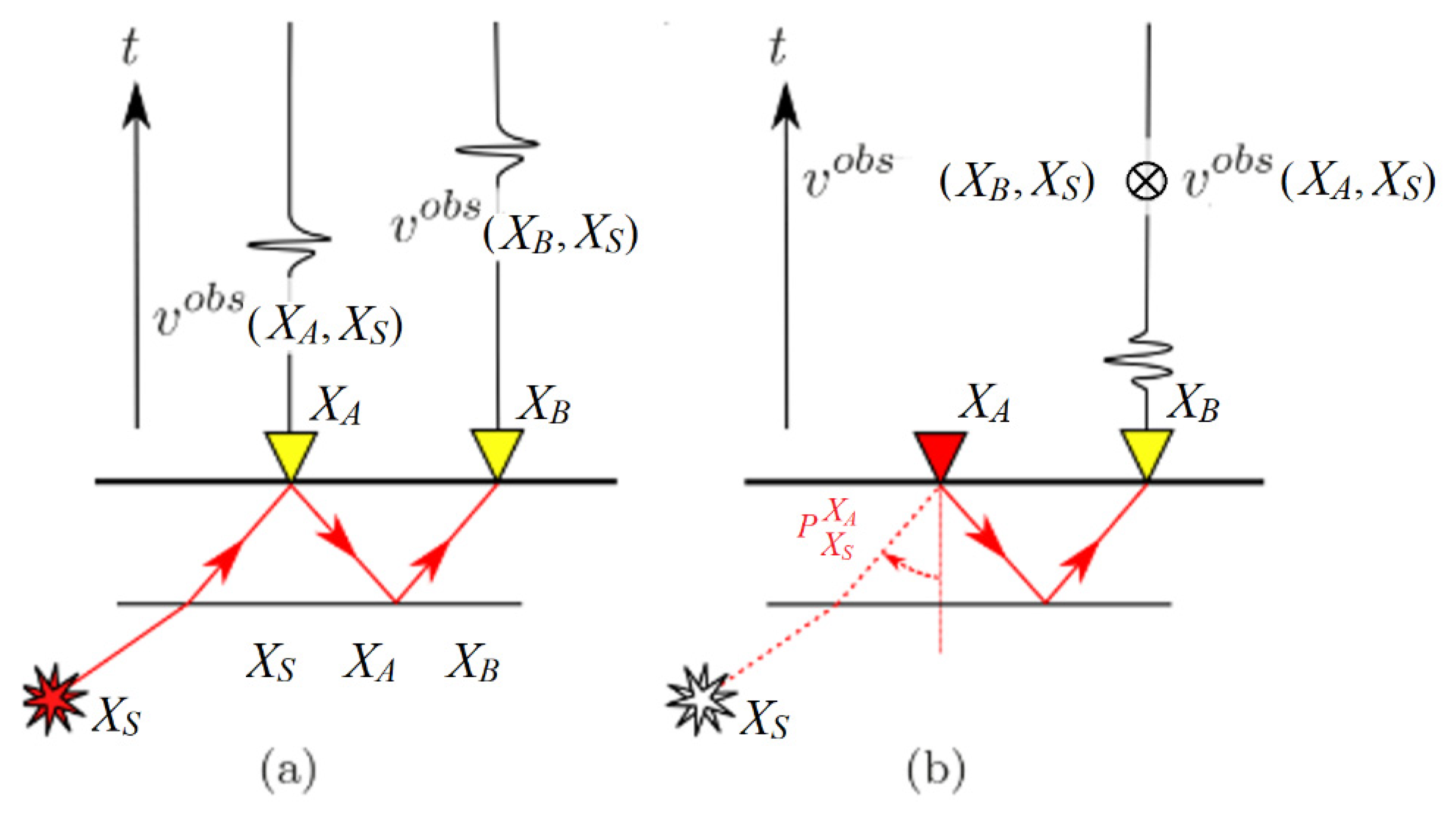
Figure 1 shows the concept described above simply. A wavefield emitted from an underground source is recorded by the geophone when the wavefield reaches the earth’s surface. Then, when the wave reflected from the earth’s surface to the underground is reflected in the earth’s surface by a scattered underground and an interface where the acoustic impedance changes are significant, this wave is recorded by another geophone. In these two figures, the path to the first geophone from underground is common. Two traces recorded by two geophones are cross-correlated, leading to the common path cancellation, while the reflection path from the first receiver to the second receiver remains. Thus, seismic reflection responses or Green’s function observed by the second geophone are obtained as if there was a source in the location of the first geophone. As a result, a virtual shot gather is obtained in a single geophone location.
The 2D finite difference wavefield modeling method was used to simulate the passive noise in the subsurface [
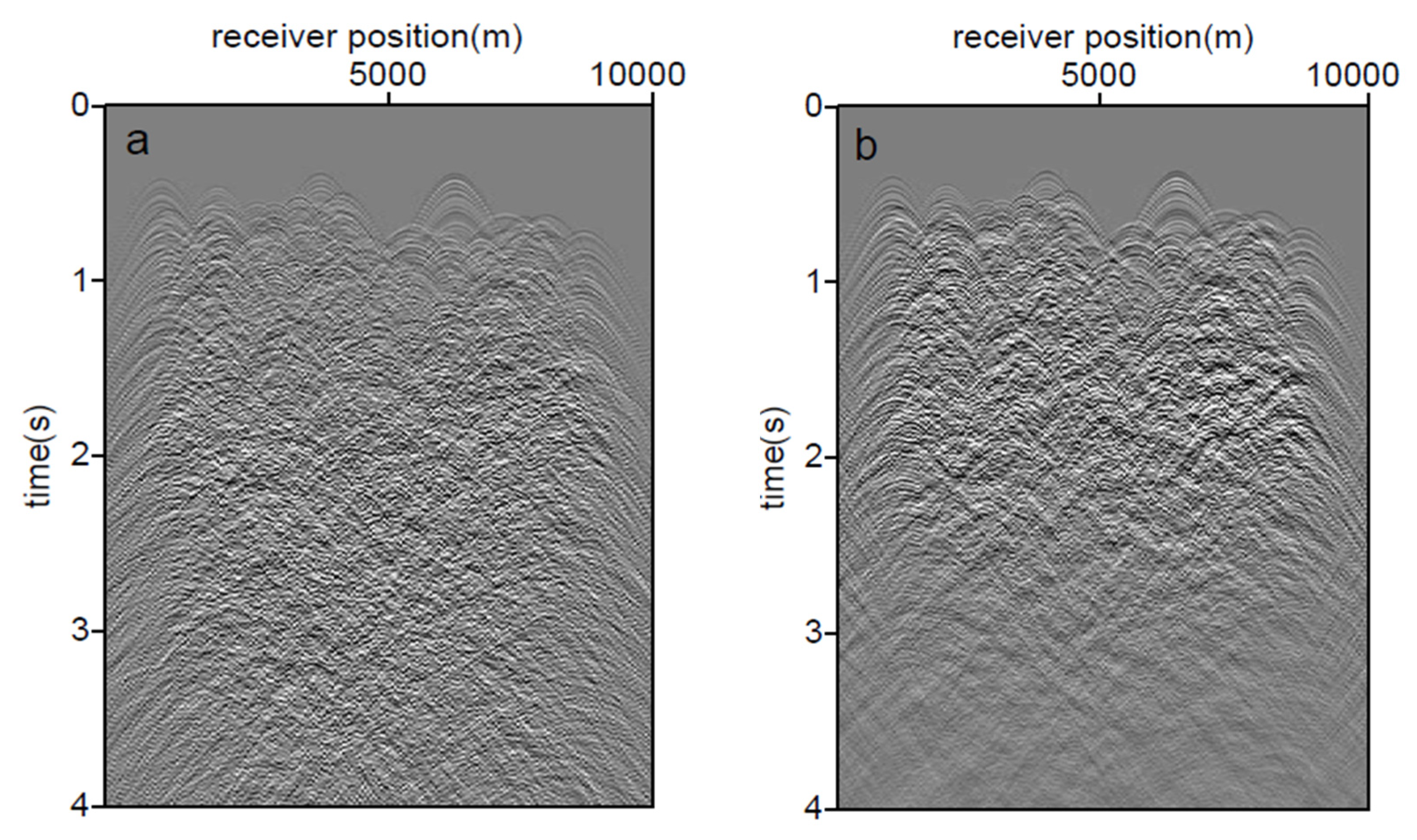
5]. In this study, acoustic scheme was used to perform the following wavefield modeling, but visco-acoustic modeling was used to investigate the effect of the weathered layer effect on the ANSI. To suppress the numerical dispersion of the finite difference in the 2D wave equation, the space and time resolution used in these simulations are 2 m and 0.001 s, respectively. A Rikers wavelet activated at a random start time and source positions with maximum frequency of 24 Hz is used for the source time function to satisfy the noninterfering impulse sources required by SI. Additionally, the first 4 s of the total 120 s long noise signals recorded in P component for the acoustic and visco-acoustic schemes are demonstrated in
Figure 2. Except of the earth arrivals, most of the source signals are interfered. To simplify the simulation, we use a global P wave Q factor 20 in the visco-acoustic scheme, from which we can see that the signal to noise ratio of the source signals from the near surface are improved.
Data Processing
Table 1 presents the workflow for the retrieval of the virtual shot gathers and the seismic stacked sections from which the geological structures subsurface can be identified. Band-pass filter and
fk filter are applied to the synthetic noise data to remove the ground roll. Following that, RMS normalization is performed to the synthetic noise. Then, one of the traces from the data is extracted as a master trace (every 5th trace) to cross-correlate against the other traces in each single gather. The location of the master trace is considered to be a virtual source for the resulting virtual “shot” gather. Cross-correlation results in causal and acausal response of Green’s function and summation over the causal and the time reversal part of the retrieved Green’s function can compensate for the incomplete illumination at two receivers [
37]. After obtaining these virtual shot gathers, we conduct conventional processing steps, including sorting to CMP gathers, conducting velocity analysis, applying NMO correction, and stacking.
3. Results
3.1. Land Acquisition below the Weathered Layer (Surface Wave Impact)
In seismic interferometry, the geophones are conventionally placed on surface. It is known that there are multiple kinds of surface noise such as traffic noise, human activities, natural sources (such as wind and stream wave), and industry vibrations that could have defective effects on retrieved reflections. Due to the close proximity of the surface noise sources and the receivers, compared with deep source signal sources relative to distant receivers, the surface noise often dominates the recorded signal in land acquisition. These surface noises, due to lack of attenuation in the path between them and the surface receivers, usually are used for passive surface wave imaging for shallow structures. This would contaminate the deep body waves ANSI [
17]; therefore, elimination of surface noise-related artefacts is critical to improving the retrieval of reflected body waves from the deep earth structures.
In the conventional data acquisition where geophones are places on the surface, a weathered layer typically exhibiting high porosity and lock of cementation acts as an attenuator of meaningful seismic signal. Usually, the low velocity and attenuating effects of the weathered layer have negative impacts on data processing procedures; however, placing the receivers beneath the weathered layer may help. Therefore, the elimination of the defective effect or taking advantage of its low-quality factor is a valuable topic for study. In this case, a visco-acoustic scheme was used for modeling, which means during the wave propagation the mechanical energy will dissipate into heat energy, to investigate the effect of weathered layer on body wave ANSI quality.
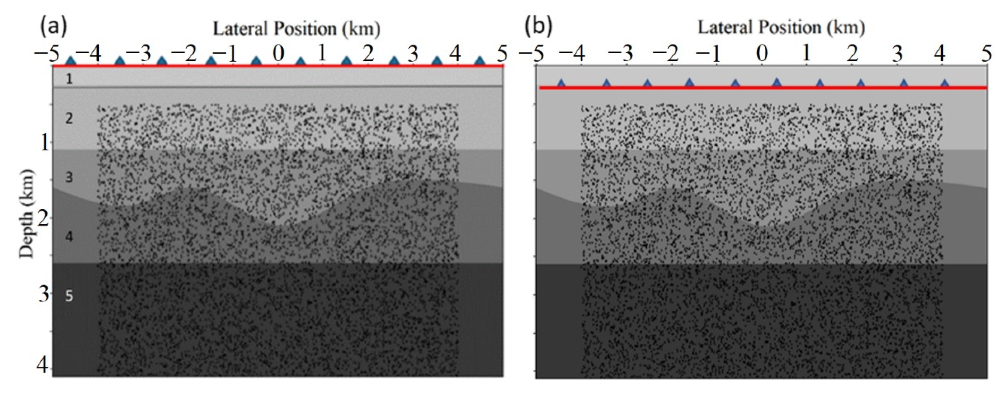
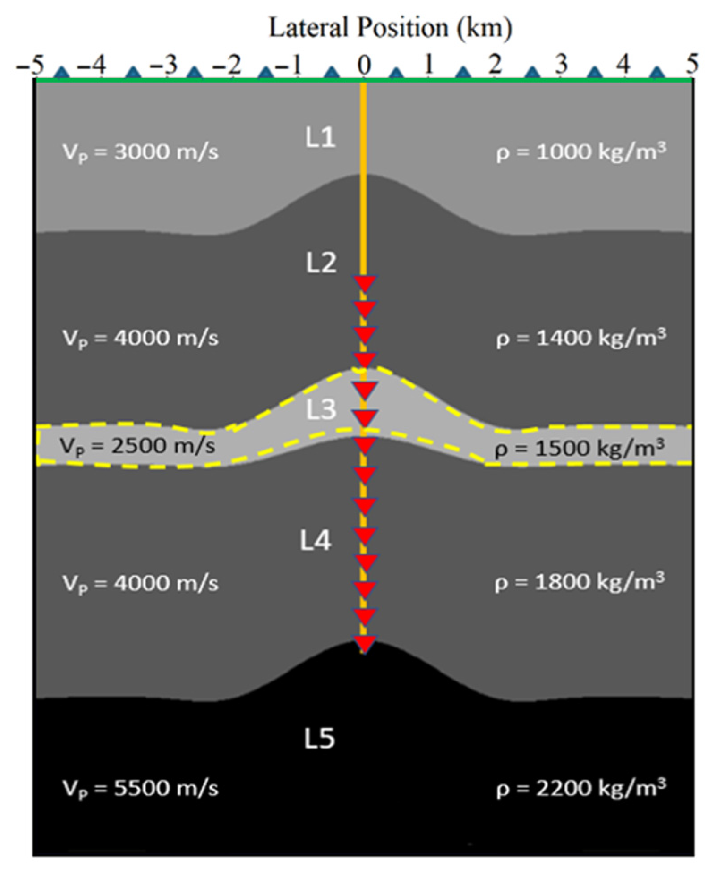
Figure 3 shows the geological models where the geophones are placed on the free surface and below the weathered layer, respectively, for comparison of the ANSI result. The uppermost layer is intended to represent the weathered layer, below which 1000 noise sources represented by black dots are randomly distributed in each model (10,000 m in width and 4100 m in depth) and are activated randomly during a period of 120 s. We intend to simulate natural sources coming from deep formations; therefore, their maximum frequency was set to 24 Hz. The 1000 sources are randomly triggered. The values of P-wave velocities and densities for different layers, with their thicknesses and two-way travel times are given in
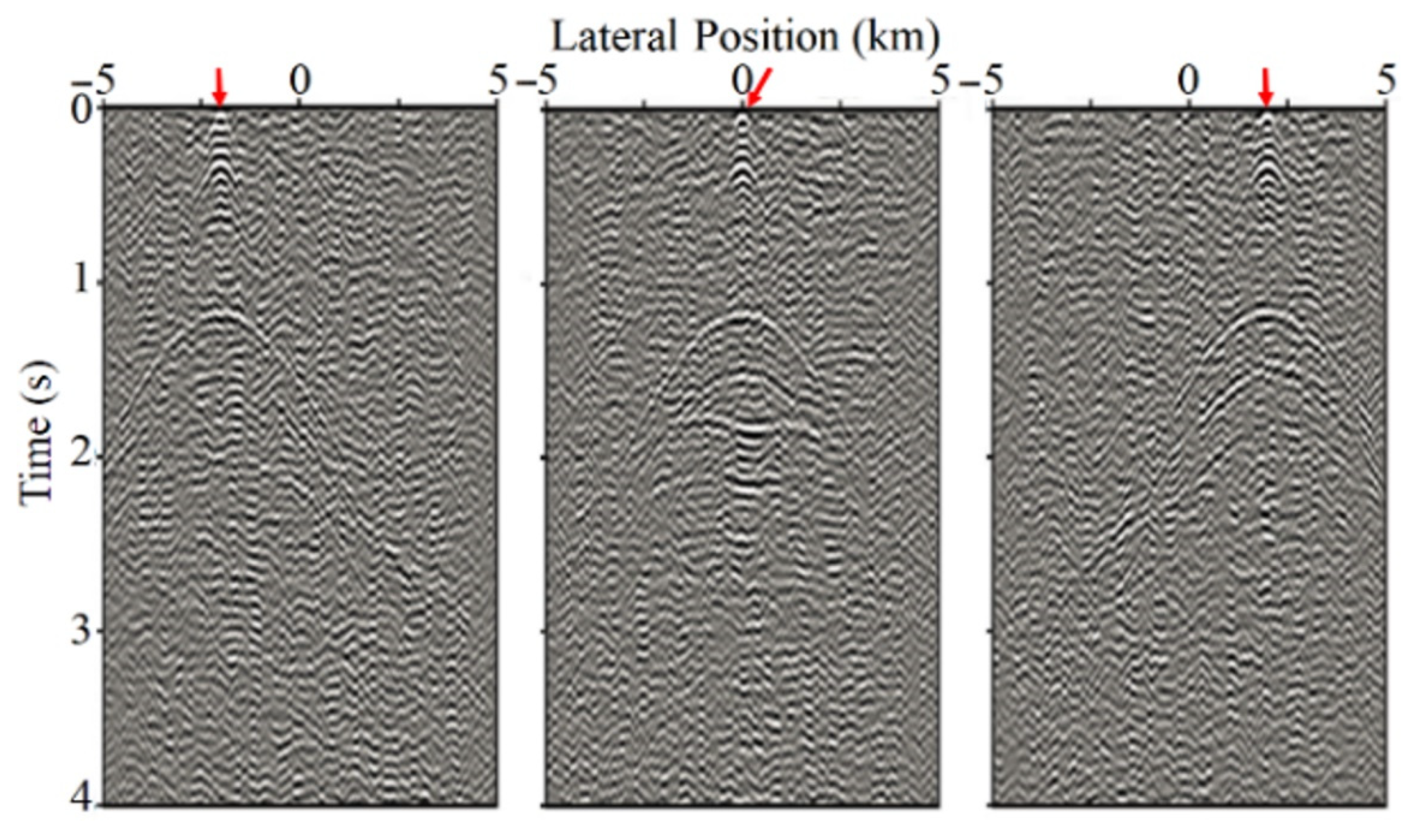
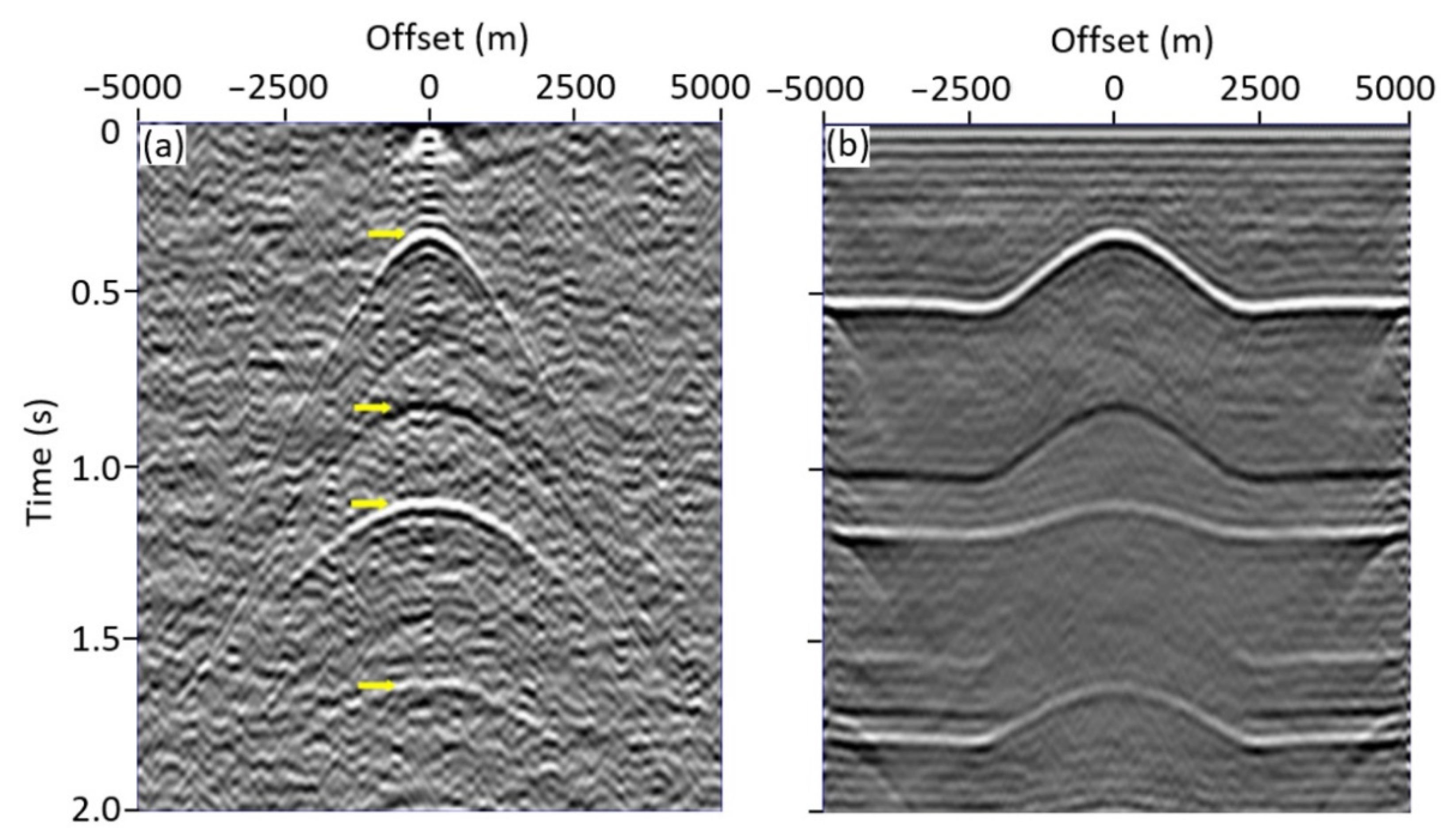
Table 2. We choose every 5th geophone (e.g., 1, 6, 11, 16, 21…) as a master trace for cross-correlation with all other traces to generate virtual shot gathers, eventually creating 201 virtual shot gathers with a 50 m shot interval in total. Each shot gather is composed of 1000 traces with a 10 m receiver interval. Three virtual shot gathers at the position of trace 301, 501, and 701 are retrieved, from which clear reflections are observed (
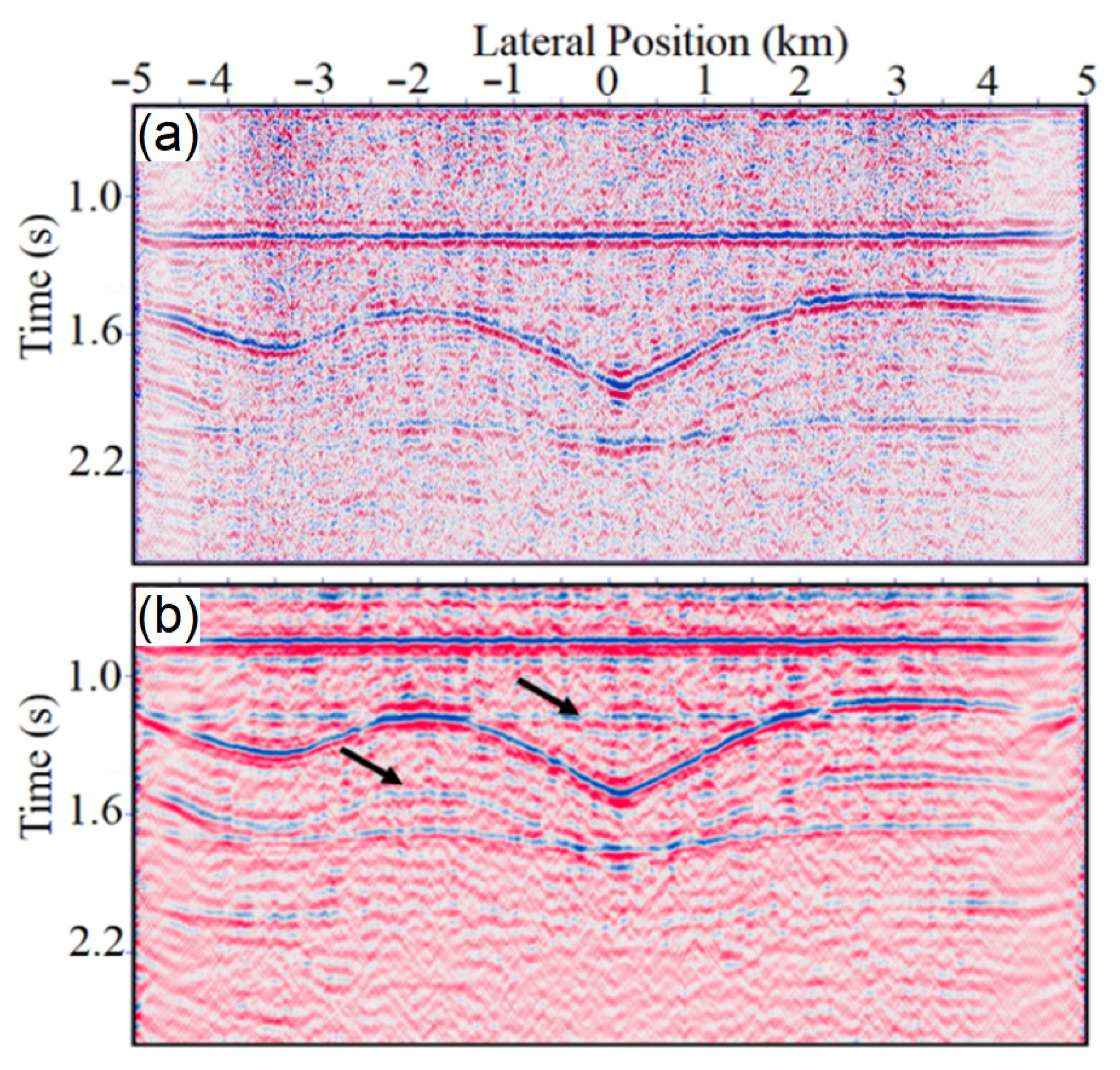
Figure 4). Because the third interface is curved, the peak of that hyperbola is not at the zero-offset position. After obtaining all the virtual shot gathers, further processing includes CDP sorting velocity analysis, normal moveout corrections (NMO), and the final stacked section before using geophones on free surface and beneath the attenuating weathered layers are shown in
Figure 5. There is no AGC or time-dependent gain applied to this section. Because the geophones are buried, the primary reflections all arrive about 0.33 s earlier on this section than their counterparts on the surface-geophone section. Note that for buried receivers, it could be obviously observed that the continuity of events has been enhanced. However, the by-product of burying the geophone is also obvious—the top reflected multiples representing the downgoing reflections from the uppermost free surface appear, mixed with some of the primary reflections. Some of them even have a tuning effect with primary reflections, which may lead to mistakes in further interpretation.
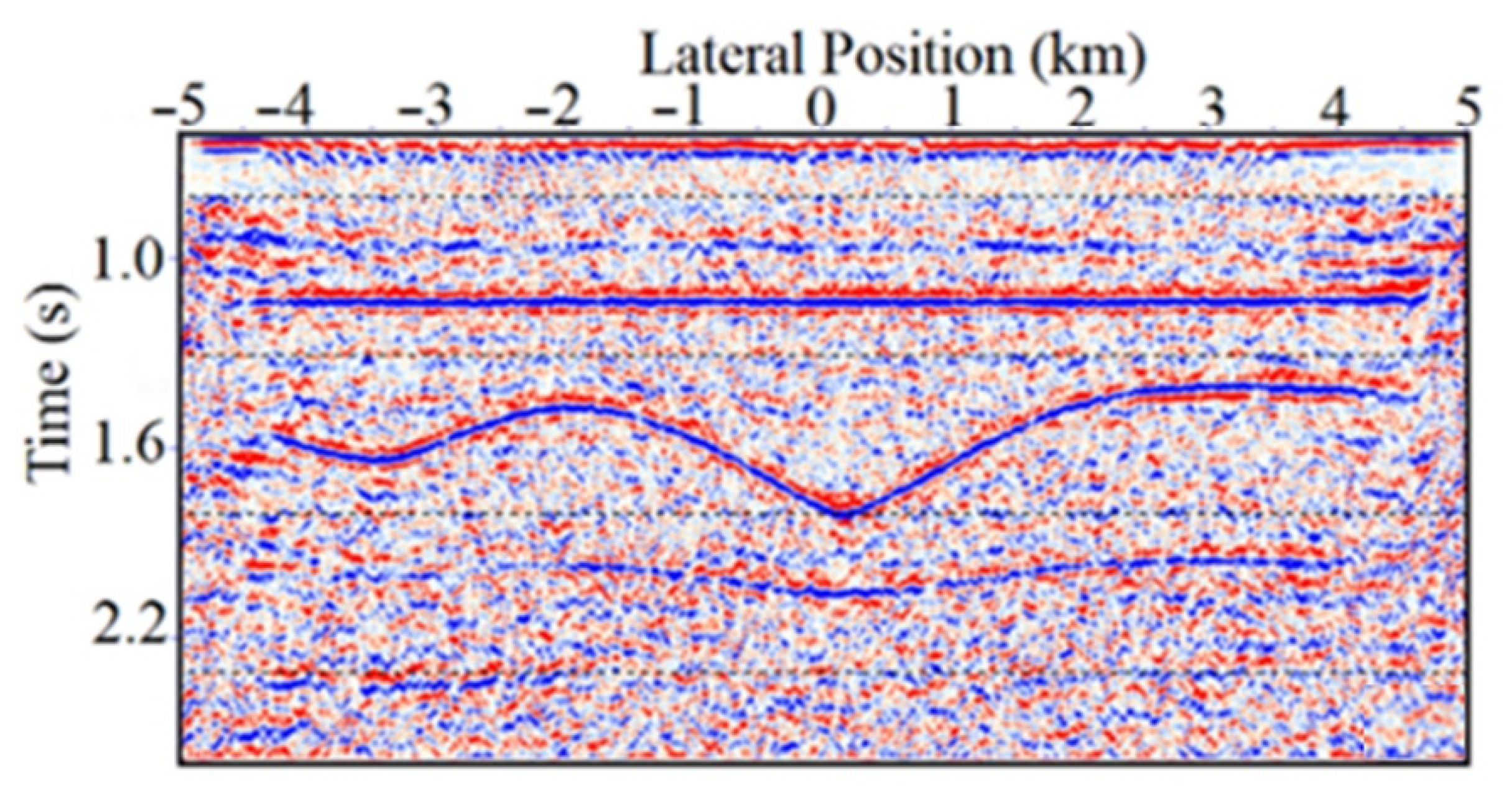
To remove the surface multiples from stacked seismic sections using buried receivers, we applied predictive deconvolution followed by a spiking deconvolution, and Hyperbolic Radon transform filter to the prestack data, yielding the section shown in
Figure 6, from which we observe that the surface multiplies have been satisfactorily removed and temporal resolution is increased.
3.2. Zero-Offset VSP Acquisition Scheme
VSP data provides the integrate information of the borehole measurements with the seismic survey. The VSP acquisition usually helps in a calibration of the surface seismic method. However, VSP data acquired using active source are costly in field. In this section, we propose the generation of the zero-offset VSP data using passive noise which reduces the budge significantly. An anticline synthetic model was used for the simulation, from which layer 3 was assigned as a coal layer with proper velocity and density values (the target area covered by yellow dashes, shown in
Figure 7). This geological model containing a total of five layers and four interfaces with anticline structures has a lateral width of 10,000 m and a depth of 4000 m. The VSP tool is positioned on the
x-axis (5000, 0) in the coordinate and has a vertical extension on the
y-axis (0, 3000) with the 101 geophones positioned in the borehole from 1000 to 3000 m depth. The surface seismic and the VSP acquisition are simultaneously operated during the simulation and 500 noise sources were randomly distributed for a 120 s recording. Following the same processing steps as in the previous section, single virtual shot gathers retrieved at the position of the middle trace and the stacked section for the surface acquisition scenario are obtained (
Figure 8).
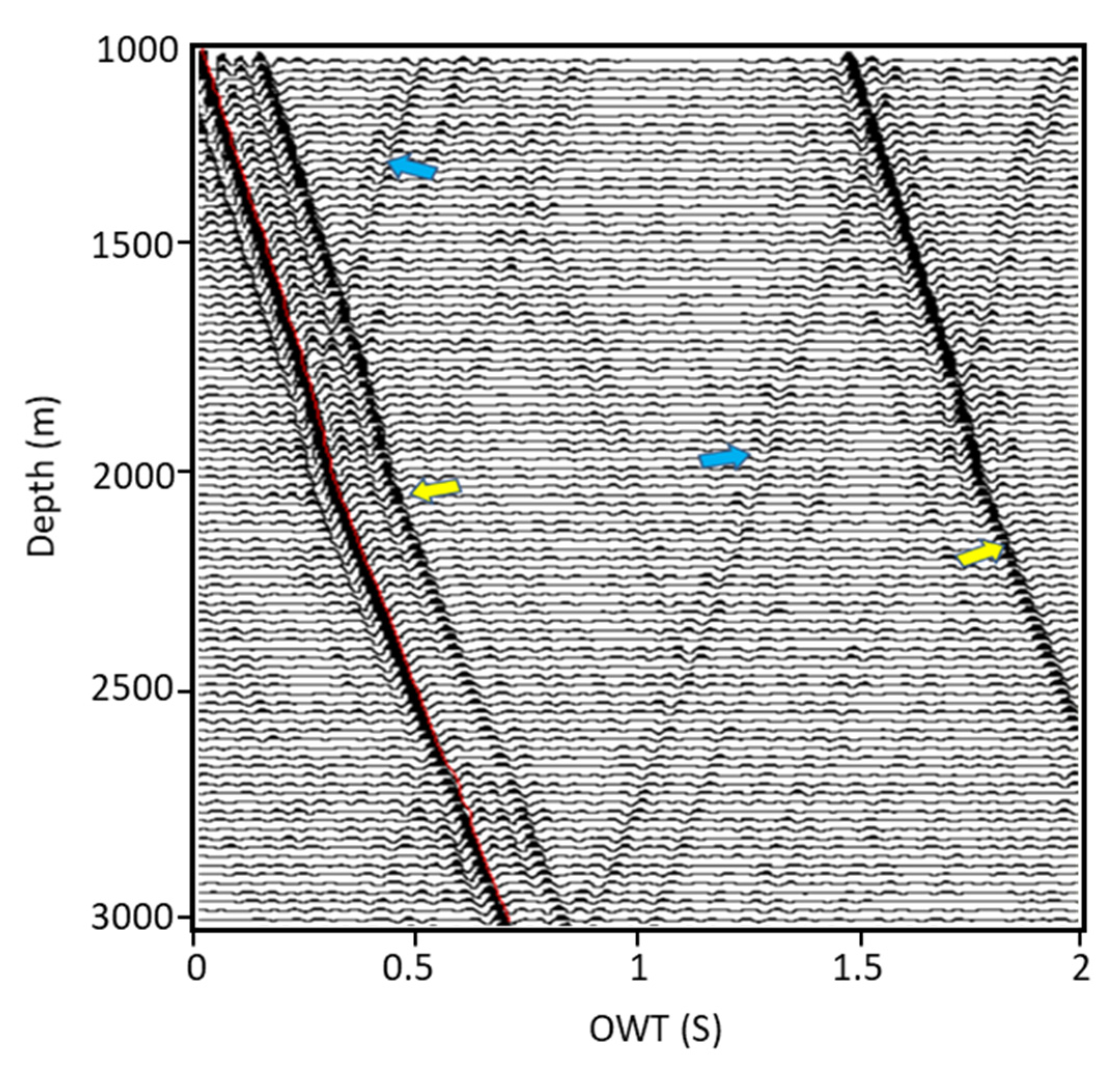
While the surface geophone measures only the upgoing waves, the VSP acquisition in the borehole records both upgoing and downgoing wavefields. After cross-correlation of the recorded noise, the time–depth conversion is applied to obtain the virtual VSP shot gather (
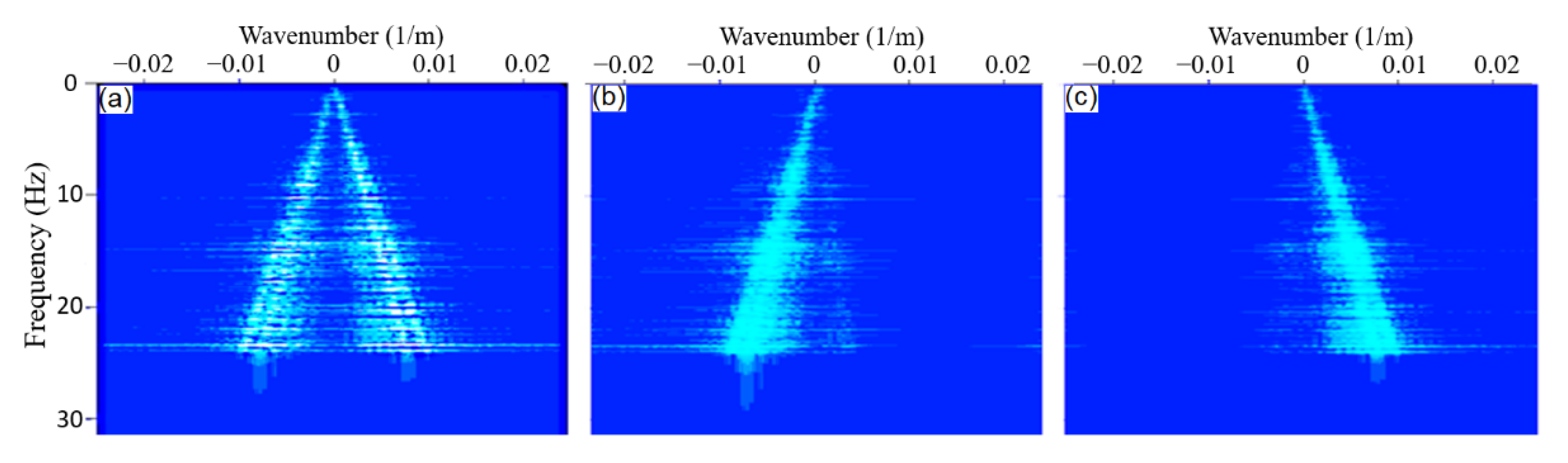
Figure 9). The primary downgoing wave or first arrival curve are picked along the red solid line, from which we see the changes in slope on this line indicate changes in velocity in the subsurface. Since the VSP data contain the downgoing wavefield and the upgoing wavefield interfering with each other, these wavefields must be decomposed. For the separation of the wavefields, frequency-wavenumber filtering is used to convert the time domain data to the frequency domain by 2D Fourier Transform. From the f-k spectra in
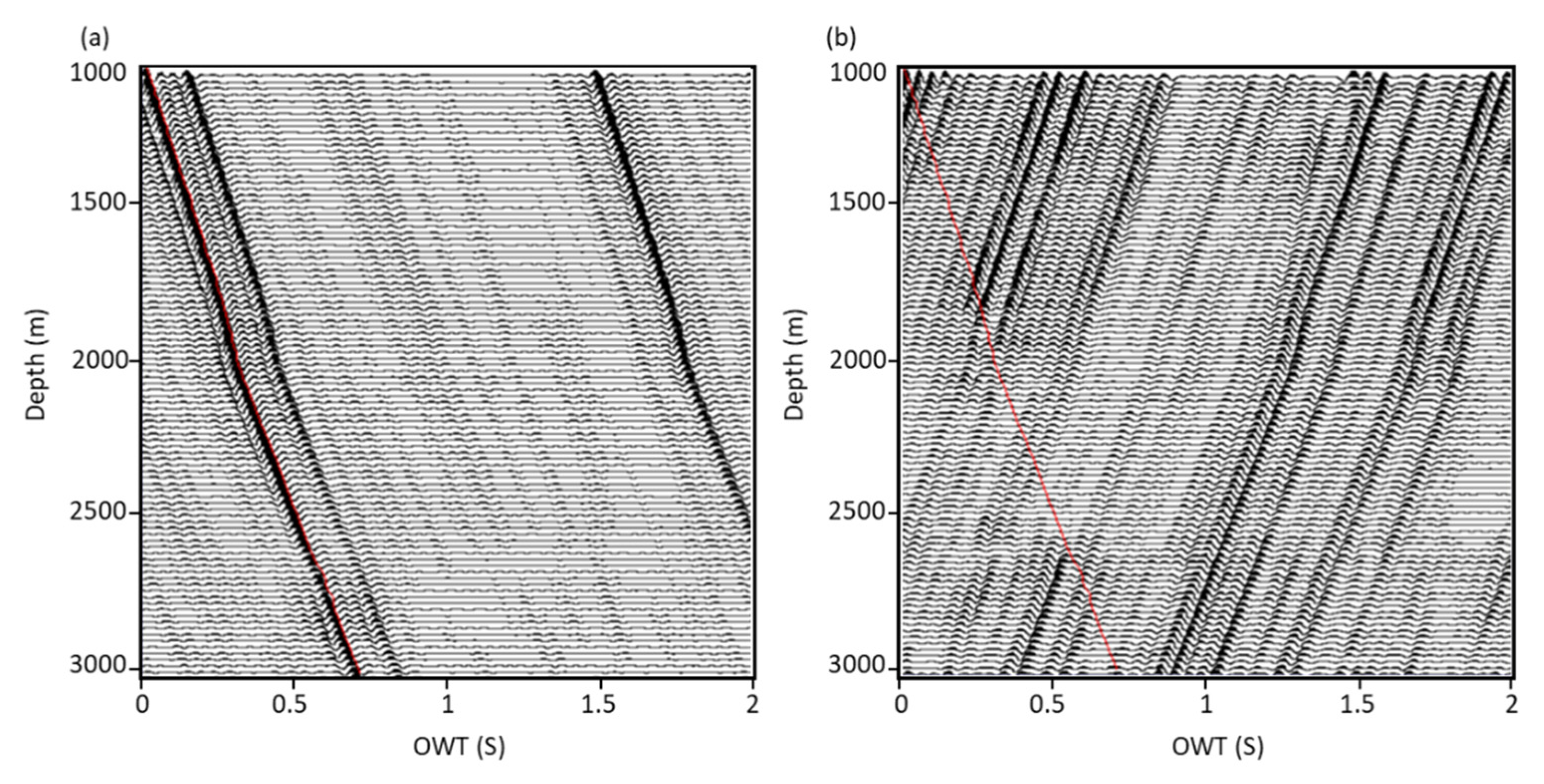
Figure 10, the downgoing wavefield has a negative slope and is located in the positive quadrant, while the upgoing wavefield is in the right side in the panel with an opposite slope. After filtering the downgoing wavefield, both wavefields are successfully obtained with a time-depth relation (
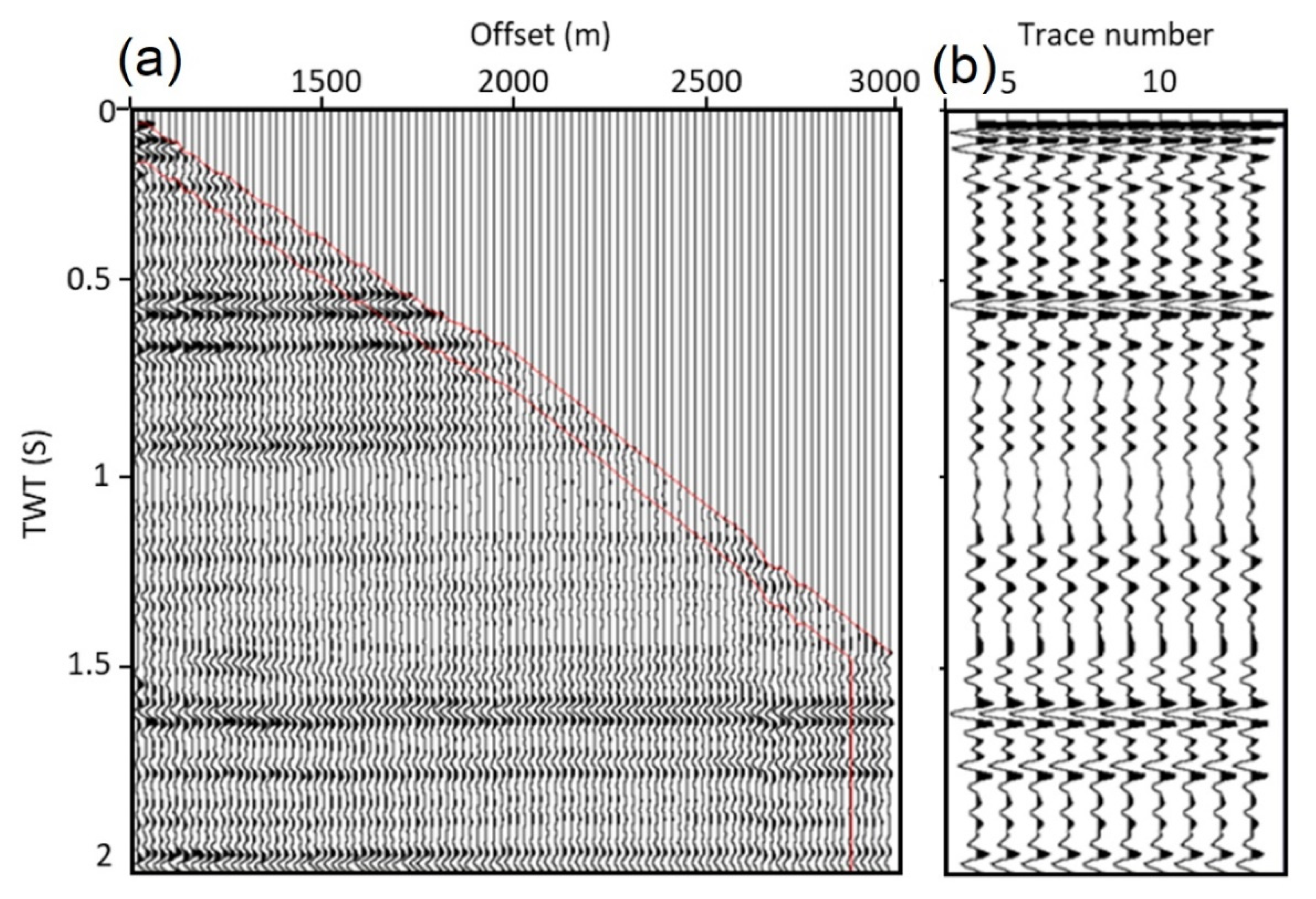
Figure 11). In the next step, static correction is carried out. All traces in the VSP data are shifted using the first arrival time. Therefore, upgoing events reduced to the time they can be recorded. Thereby, all traces in the upgoing wavefield are aligned and flattened (
Figure 12). Thus, one-way time is transformed into two-way travel time (TWT). At last, the flattened upgoing wavefield is used for building corridor stacks, which can be used to compare the surface seismic acquisition result. The traces are stacked using the outside corridor stack because of it is multiple-free and has only primary events.
3.3. Crosswell Seismic Acquisition Geometry
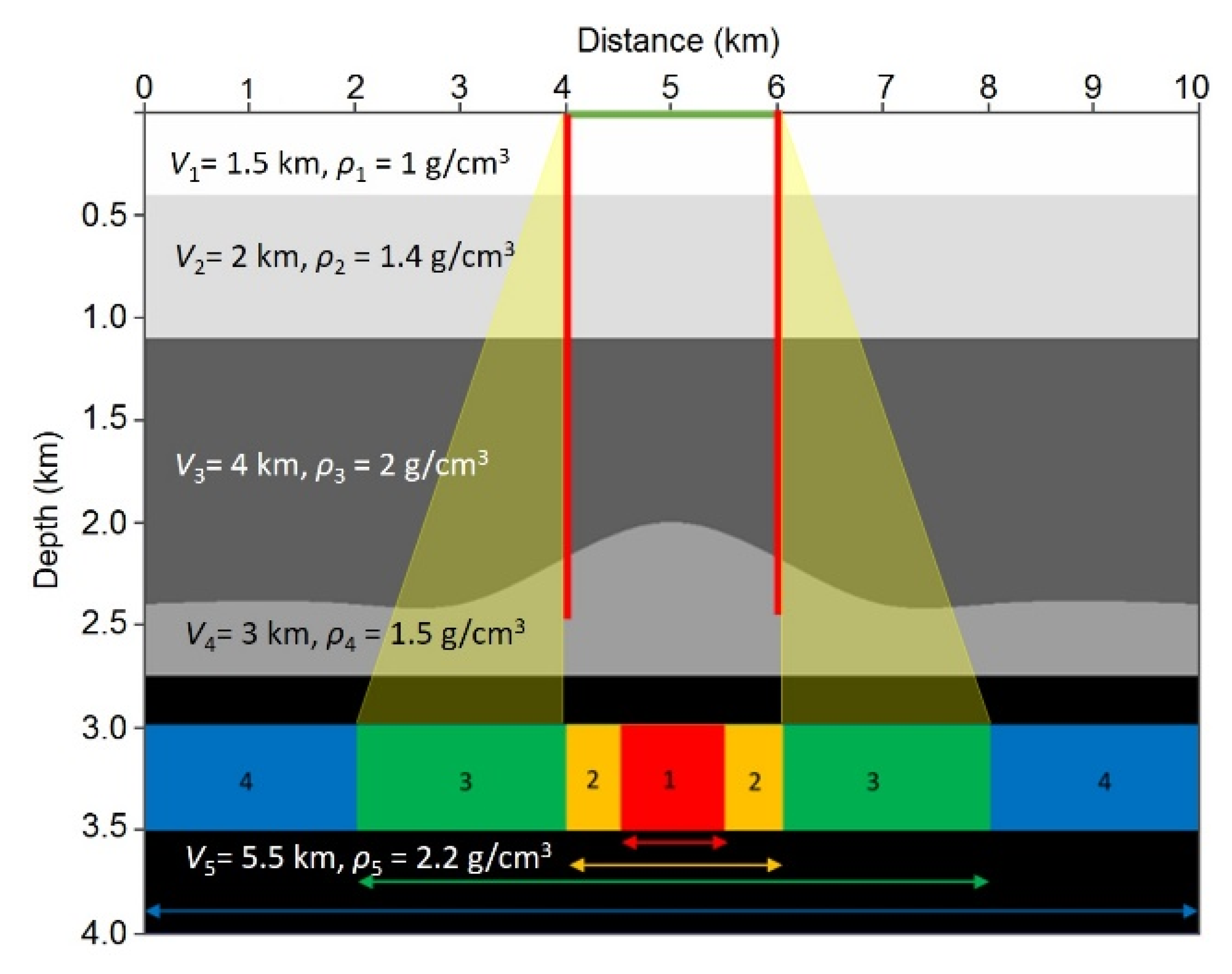
Crosswell survey, where the source points are location in one borehole and the receiver array is located in a second borehole, can be referred as a special case of the VSP survey (
Figure 13). The term crosswell comes from the transverse ray paths that arise when measurements are made between two boreholes. In the ANSI application from the crosswell survey, the sources are positioned at different depths and gradually detonated. This creates a good ray overlap between the drilling holes. With the crosswell measurements, the area between two boreholes can therefore be investigated. Typically, tomographic methods that are used here to evaluate the travel times between the sources are receivers so that the two-dimensional distribution of the propagation velocity can be determined.
In this section, a simple layered model with a buried mound was created with the geometry and parameters shown in
Figure 13 with the additional information concerning the representation of the four different noise boundaries. Two wells (vertical red lines) were placed on the flanks of the mound to be used for crosswell data acquisition. The green line in
Figure 13 represents the location of a surface array. We adopt noise boundary models proposed by [
7]. This model contains 1000-point sources of noise that occur pseudo-randomly in space and time within a specified spatial boundary.
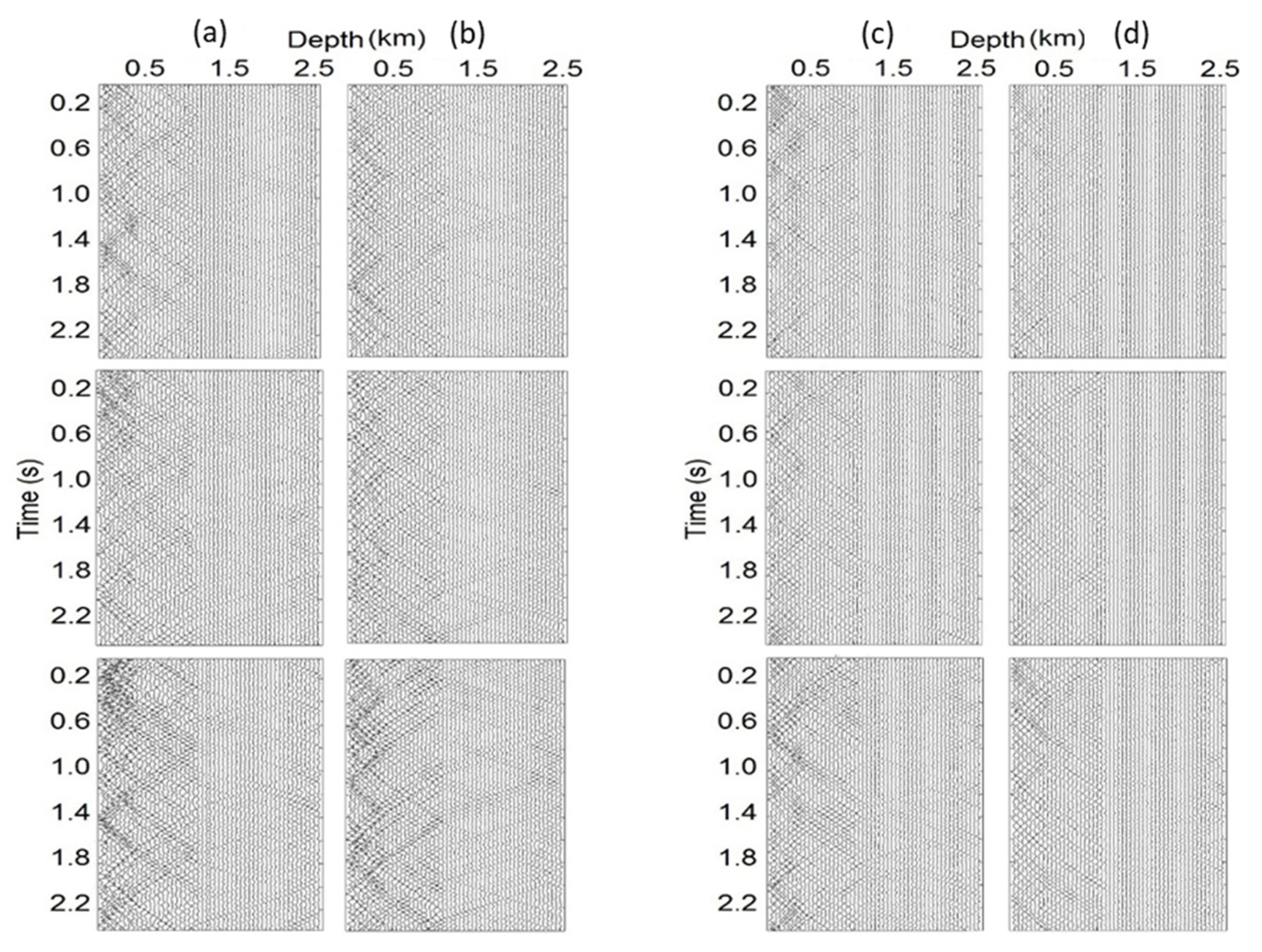
For the crosswell acquisition, the top geophone in the left-side array is selected as the master trace, and cross-correlated will all of the geophones in the right-side array, one at a time, indexing down the virtual well. In this way, a crosswell common-source gather is produced. The geophone selected for the master trace is then indexed one location down in the left side well and used for cross-correlation with all of the geophones in the right side well, indexing down the well. This process continues until every geophone in the left side array was used as a master trace for a virtual shot gather. Although the validity of the process of cross-correlation in a surface setting has been demonstrated in others, the process fails when it is applied to crosswell data.
This can be seen in
Figure 14, where the difference gathers are larger amplitude than either the base or repeat surveys themselves, representing essentially no similarity between the two surveys, even though the models were identical. There are no obvious reflectors visible in either the base or repeat surveys, and the differential between them yields a strong and seemingly arbitrary set of events. In this instance, cross-correlation does not stack a coherent image from random points of ambient noise in the subsurface. It has been shown elsewhere that SI can be utilized for a crosswell acquisition for an active source at the surface, but it was postulated that the use of random noise in the subsurface would create too complex a geometrical problem, as the source times and locations are unknown [
38].
The major problem for crosswell applications of SI using buried noise sources appears to result from an inability to stack the reflector information in a coherent way. For example, cross-correlation works well with a surface array geometry because the geophones used for cross-correlation are near to each other and at nearly the same distance from the (distant) noise volume. Therefore, upon cross-correlation, the traces are quite similar to each other, and the reflector responses stack nicely. In the crosswell case, where a geophone at the surface is being cross-correlated with geophones that are very near the noise source, or vice versa, the traces are highly dissimilar. This complicates cross-correlation, which depends on the bulk travel of raypaths being similar from the source to the geophone pair. The response from a given reflector will be significantly different at geophones in different layers in both amplitude and time, thereby making cross-correlation inappropriate.
4. Discussions
We used acoustic modeling to assess different data acquisition scenarios for better retrieval of body waves from ANSI. In general, acoustic modeling can provide some approximate behavior of seismic data in particular for body wave simulations as it is the main theme of the present research. Acoustic modeling can provide reasonable results in the case of short-offset data acquisitions, or in other words, the incident angle of seismic waves is close to the right angle. Therein lies the reason why acoustic modeling for the simulation of body wave data has been used by many researchers, e.g., [
4,
17,
27]. However, in reality, body waves are not simply P-waves but includes S-waves and reflected/transmitted/converted P/S S/P waves. In particular, in long offset P-wave data acquisitions where the incident angles of P-waves vary from 0° to 90°, in addition to the reflected and transmitted P-waves, two converted reflected and transmitted S-waves are generated. Moreover, in the case of surface conditions, we should expect the generation of surface waves, i.e., ground rolls and Love wave. Therefore, a more robust evaluation of different seismic data acquisition scenarios should be achieved via a visco-elastic modeling (considering Vp, Vs, Qp, Qs, and ρ parameters) instead of visco-acoustic modeling, which is incapable of modeling converted or surface waves. Providing that we consider the visco-elastic modeling, we can better evaluate the performance of various data acquisition methods. For instance, in our simulations pertinent to land acquisition below the weathered layer, the visco-elastic modeling will more effectively show the advantage of placing receivers below the weathered layer because the surface ambient noises are mostly dominated by surface waves that dramatically decay with depth (note that in acoustic modeling they are modeled as body waves that are not significantly attenuated with depth). We also should expect that for crosswell seismic acquisition geometry, the visco-elastic modeling will present further disadvantage of this data acquisition configuration for the retrieval of P-wave from ANSI since in this wide-angle data acquisition, a fraction of P-wave energy is converted to S-waves. Therefore, the retrieved P-waves will be much weaker than what we obtained through our acoustic modeling. On the other hand, for the zero-offset VSP acquisition scheme, we do not anticipate a significant difference in acoustic and visco-elastic modeling because of narrow angle (short offset) of data acquisition. In this case, no strong converted P-wave is generated, and therefore, acoustic and visco-elastic modeling will provide the same results.
Furthermore, it is well known that the ambient noise is dominated by surface waves and it should imply a complete wavefield modeling. Incidentally, we did not consider surface waves given the frequency range that we process the data in this study (e.g., 6–24 Hz).


